Cluster emission and phase transition behaviours in nuclear disassembly

Abstract

The features of the emissions of light particles (LP), charged particles (CP), intermediate mass fragments (IMF) and the largest fragment (MAX) are investigated for ${}^{129}Xe$ as functions of temperature and ’freeze-out’ density in the frameworks of the isospin-dependent lattice gas model and the classical molecular dynamics model. Definite turning points for the slopes of average multiplicity of LP, CP and IMF, and of the mean mass of the largest fragment ( $A_{max}$ ) are shown around a liquid-gas phase transition temperature and while the largest variances of the distributions of LP, CP, IMF and MAX appear there. It indicates that the cluster emission rate can be taken as a probe of nuclear liquid–gas phase transition. Furthermore, the largest fluctuation is simultaneously accompanied at the point of the phase transition as can be noted by investigating both the variances of their cluster multiplicity or mass distributions and the Campi scatter plots within the lattice gas model and the molecular dynamics model, which is consistent with the result of the traditional thermodynamical theory when a phase transition occurs.

I Introduction

Phase transition and critical phenomenon is an extensively debatable subject in the natural sciences. Recently, the same concept was introduced into the astronomical objects [1] and the microscopic systems, such as in atomic cluster [2] and nuclei [3], of these the nuclei, as a microscopic finite-size system, are attracting more and more nuclear experimentalists to search for the liquid–gas phase transition and investigate their behaviour. To date, various experimental evidences have cumulated which seem to be related to the nuclear phase transition. For instance, violent heavy-ion collisions break the nuclei into several intermediate mass fragments, which can be viewed as a critical phenomenon as observed in fluid, atomic and other systems. It prompts a possible signature on the liquid–gas phase transition in the nuclear system. The sudden opening of the nuclear multifragmentation and vaporization [4] channels can be interpreted as the signature of the boundaries of phase mixture [5]. In addition, the plateau of the nuclear caloric curve in a certain excitation energy range gives a possible indication of a first-order phase transition [6, 7] as predicted in the framework of statistical equilibrium models [8]. On the other hand, the extraction of critical exponents in the charge or mass distribution of the multifragmentation system [9] can be explained as an evidence of phase transition. More recently, the negative microcanonical heat capacity was experimentally observed in nuclear fragmentation [10] which relates to the liquid–gas phase transition [11], and in atomic cluster [12] which relates to solid to liquid phase transition [13], respectively. Moreover, some evidence of spinodal decomposition in nuclear multifragmentation was recently obtained experimentally [14], which shows the presence of liquid–gas phase coexistence region and gives a strong argument in favour of the existence of first-order liquid–gas phase transition in finite nuclear systems.

Meanwhile, several theoretical models have been developed to treat such a phase transition in the nuclear disassembly, e.g. percolation model, lattice gas model, statistical multifragmentation model and molecular dynamics model etc (e.g. see the recent review article of Richert and Wagner [15] and references therein). In this paper, we are interested in the lattice gas model ( LGM ) and classical molecular dynamics ( CMD ) model [16]. The former is a simple short range interaction model [17], but it can successfully be applied to nuclear systems with isospin symmetry and asymmetry. LGM is carried assuming that the system is in a ’freeze-out’ density $\rho_{f}$ with thermal equilibrium at temperature T. Previous calculations [18] with LGM showed that there exists a phase transition for the finite nuclear systems by studying the effective power law parameter ( $\tau$ ) of cluster mass or charge distribution, their second moments ( $S_{2}$ ) and the specific heat. More recently, we proposed two novel criteria, namely multiplicity information entropy ( $H$ ) and nuclear Zipf’s law to diagnose the onset of liquid–gas phase transition in the framework of the isospin-dependent LGM (I-LGM) and isospin-dependent classical molecular dynamics (I-CMD) model [19].

In this paper, we show that the emission rate of clusters is a useful tool to diagnose the nuclear liquid–gas phase transition, while the largest fluctuation of cluster multiplicities is simultaneously revealed at the point of the phase transition by investigating the features of light particles (LP), charged particles (CP), intermediate mass fragments (IMF) and the largest fragment (MAX) of disassembling source in I-LGM and I-CMD frameworks.

The paper is organized as follows. Section 2 gives the descriptions of I-LGM and I-CMD. Results and discussions are shown in section 3 where the multiplicities of cluster emissions, their slopes and their fluctuations are investigated. The influence of the ’freeze-out’ density on cluster emission is also presented in the framework of I-LGM and I-CMD and the role of Coulomb interaction is studied by comparing the results of I-LGM and I-CMD at a given ’freeze-out’ density. Finally, the conclusion is given in section 4.

II Description of models

II.1 Isospin-dependent lattice gas model

The lattice gas model of Lee and Yang [17], where the grand canonical partition function of a gas with one type of atoms is mapped into the canonical ensemble of an Ising model for spin 1/2 particles, has successfully described the liquid–gas phase transition for the atomic system. The same model has already been applied to the microscopic nuclear system, e.g. see the papers of Pan and Das Gupta et al [16]. In order to better understand the context of this study, the models are described below.

In the LGM, A ( = N + Z ) nucleons with an occupation number s which is defined as the ‘spin’ s = 1 ( -1 ) for a proton (neutron) or s = 0 for a vacancy, are placed in the L sites of a, three-dimensional cubic lattice. Each cubic lattice has a size 1.0/$\rho_{0}$ = 6.25 $fm^{3}$ and can, at most, be occupied by a single nucleon, where $\rho_{0}$ = 0.16 $fm^{-3}$ is the normal nucleon density. Nucleons in the nearest neighbouring sites interact with an energy s i s j. The Hamiltonian of the system is written as

$$H=\sum_{i=1}^{A}\frac{P_{i}^{2}}{2m}-\sum_{i<j}\epsilon_{s_{i}s_{j}}s_{i}s_{j}.$$ (1)

The interaction constant $\epsilon_{s_{i}s_{j}}$ is related to the binding energy of the nuclei. In order to incorporate the isospin effect in the LGM, the short-range interaction constant $\epsilon_{s_{i}s_{j}}$ is chosen to be different between the nearest neighbouring like nucleons and unlike nucleons,

$$\epsilon_{nn}\ = \ \epsilon_{pp}\ =\ 0.MeV,$$

$$\epsilon_{pn}\ = \ -5.33MeV,$$ (2)

which indicates the repulsion between the nearest-neighbouring like nucleons and attraction between the nearest-neighbouring unlike nucleons. This kind of isospin-dependent interaction incorporates, to a certain extent, the Pauli exclusion principle and effectively avoids producing unreasonable clusters, such as di-proton and di-neutron clusters etc. The disassembly of the system is calculated at an assumed ‘freeze-out’ density $\rho_{f}$ = (A/L)$\rho_{0}$ , beyond $\rho_{f}$ nucleons are too far apart to interact.

In this model, N + Z nucleons are put in L sites by Monte Carlo sampling using the canonical Metropolis algorithm [20]. As pointed out in [21], however, one has to be careful treating the process of Metropolis sampling in order to satisfy the detailed balance principle and therefore warrant the correct equilibrium distribution in the final state. Describing in detail, in this paper, first an initial configuration with N + Z nucleons is established. Second, for each event, a sufficient number of ’spin’-exchange steps are tested, e.g. 20 000 steps to let the system generate states with a probability proportional to the Boltzmann probability distribution with the Metropolis algorithm. In each ’spin’-exchange step, a random trial change on the basis of the previous configuration is made. For instance, we choose a nucleon at random and attempt to exchange it with one of its neighbouring nucleons or vacancies regardless of the sign of its ’spin’ (Kawasaki-like spin-exchange dynamics [22]), then compute the change $\Delta E$ in the energy of the system due to the trial change. If $\Delta$E is less than or equal to zero, accept the new configuration and repeat the next ’spin’-exchange step. If $\Delta E$ is positive, compute the ’transition probability’ W = $e^{-\Delta E/T}$ and compare it with a random number r in the interval [0, 1]. If r $\leq$ W , accept the new configuration, otherwise retain the previous configuration. Twenty thousand ’spin’-exchange steps are performed to ensure that we get that the equilibrium state (afterwards we will show the ’spin’-xchange step dependence of some observables). Third, once the nucleons have been placed stably on the cubic lattice after 20000 ’spin’-exchange steps for each event, their momenta are generated by Monte Carlo sampling of the Maxwell–Boltzmann distribution. Thus various observables based on phase space can be calculated in a straightforward fashion for each event. One important point of such Monte Carlo Metropolis computations is that the above ’spin’-exchange approach between the nearest neighbors, independently of their ’spin’, is evidenced to be satisfied by the detailed balance condition as noted in [21]. In other words, this sampling method guarantees that the generated microscopic states form an equilibrium canonical ensemble.

Once this is done the LGM immediately gives the cluster distribution by using the rule that two nucleons are part of the same cluster if their relative kinetic energy is insufficient to overcome the attractive bond [18]:

$$P_{r}^{2}/2\mu-\epsilon_{s_{i}s_{j}}s_{i}s_{j}<0.$$ (3)

This method has been proved to be similar to the so-called Coniglio–Klein prescription in condensed matter physics [23] and was shown to be valid in LGM.

II.2 Isospin-dependent classical molecular dynamics model

Since the LGM is a model of the nearest-neighbouring interaction, a long-range Coulomb force is not amenable to lattice gas type calculation. Pan and Das Gupta [16, 17] provide a prescription, based on simple physical reasoning, to decide if two nucleons, occupying neighbouring sites form part of the same cluster or not [26]. They first try to map the LGM calculation to a molecular dynamics type prediction, both first carried out without any Coulomb interaction. If the calculations match quite faithfully, then they can study the effects of the Coulomb interaction by adding that to the molecular dynamics calculation. Here we adopt the same prescription to use the molecular dynamics and therefore investigate the Coulomb effect. The results and conclusions are now compared and checked between the LGM and the CMD.Obviously, here we do not perform any ab initio molecular dynamics calculation but only use it for simulating the nuclear disassembly, starting from a thermally equilibrated source which has been produced by the above I-LGM: i.e. the nucleons are initialized at their lattice sites with Metropolis sampling and have their initial momenta with Maxwell– Boltzmann sampling. From this starting point we switch the calculation to CMD evolution under the influence of a chosen force. Note that in this case $\rho_{f}$ is, strictly speaking, not a ‘freeze-out’ density for molecular dynamics calculation but merely defines the starting point for time evolution. However, since classical evolution of a many particle system is entirely deterministic and the initialization does have in it all the information of the asymptotic cluster distribution, we continue to call $\rho_{f}$ the ’freeze-out’ density.

The form of the force in the CMD is also chosen to be isospin dependent in order to compare with the results of I-LGM. The potential for unlike nucleons is expressed as [16, 24]

$$v_{\rm np}(r)(r/r_{0}<a)\ = \ C\left[B(r_{0}/r)^{p}-(r_{0}/r)^{q}\right]exp({\frac{1}{(r/r_{0})-a}}),$$

$$v_{\rm np}(r)(r/r_{0}>a)\ = \ 0.$$ (4)

where $r_{0}$ = 1.842 fm is the distance between the centres of two adjacent cubes so that $\rho_{0}$ = 1/${r_{0}}^{3}$ = 0.16 $fm^{-3}$. The parameters of the potentials are p = 2, q = 1, a = 1.3, B = 0.924 and C = 1966 MeV. With these parameters the potential is minimum at $r_{0}$ with the value -5.33 MeV, zero when the nucleons are more than 1.3$r_{0}$ apart and strongly repulsive when r is significantly less than $r_{0}$ . We now turn to the nuclear potential between like nucleons. Although we take $\epsilon_{pp}$ = $\epsilon_{nn}$ = 0 in I-LGM, the fact that we do not put two like nucleons in the same cube suggests that there is short-range repulsion between them. We have taken the nuclear force between two like nucleons to be the same expressions as above +5.33 MeV up to r = 1.842 fm and zero afterwards,

$$v_{\rm pp}(r)(r<r0)\ = \ v_{\rm np}(r)-v_{\rm np}(r_{0}),$$

$$v_{\rm pp}(r)(r>r0)\ = \ 0.$$ (5)

Figure 1 shows the above potential $v_{np}$ or $v_{pp}$. This potential form automatically cuts off at r/$r_{0}$ = a (equation (4)) or r/$r_{0}$ = 1 ( equation (5) ) without discontinuities in any r derivatives, which is a distinct advantage in any molecular dynamics simulation application.

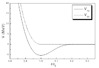
Figure 1: Molecular dynamics potential for like nucleon pair ( $v_{pp}$ ) and unlike nucleon pair ( $v_{np}$ ).

The system evolves with the above potential. The time evolution equations for each nucleon are, as usual, given by

$$\partial\vec{p_{i}}/\partial t\ = \ -\Sigma_{j\neq i}\bigtriangledown_{i}v(r_{ij}),$$

$$\partial\vec{r_{i}}/\partial t\ = \ \vec{p_{i}}/m.$$ (6)

Numerically, the particles are propagated in the phase space by a well-known Verlet algorithm [25], one of the finite-difference methods in molecular dynamics with continuous potentials. At asymptotic times, for instance, the original blob of matter expands to 64 times its volume in the initialization, the clusters are easily recognized: nucleons which stay together after an arbitrarily long time are part of the same cluster. The observables based on cluster distribution in both models are now compared while they are also compared by switching on/off the Coulomb interaction within the molecular dynamics.

III Results and discussions

We choose a medium-size nucleus ${}^{129}Xe$ as an example. The input parameters are temperature T and ’freeze-out’ density $\rho_{f}$ in the model calculations. In this study T is mostly limited to the range of 1.5–7 MeV and the ’freeze-out’ density $\rho_{f}$ changes in a wide range, namely, 0.097$\rho_{0}$, 0.18$\rho_{0}$, 0.38$\rho_{0}$ and 0.60$\rho_{0}$, which corresponds to the total cubic lattices $11\times 11\times 11$, $9\times 9\times 9$, $7\times 7\times 7$ and $6\times 6\times 6$, respectively, of which, 0.60$\rho_{0}$ is the maxmium freeze-out density which is allowed for ${}^{129}Xe$ because a cubic lattice is required in our LGM calculations. One thousand events are simulated for each combination of T and $\rho_{f}$ which ensures good statistics for results.

Before we present the results, we would like to check the role of the ’spin’-exchange step and from that we can know how the system tends to the equilibrium state in the model. Suppose, we wish to determine experimentally the value of a property of a system such as internal energy or cluster emission. In general, such properties depend upon the phase space of A nucleons. Over time, the instantaneous value of the property fluctuates as a result of interactions between the nucleons. However, when the system reaches its equilibrium state, the average of the instantaneous values over huge samples (‘ensemble average’) are viewed as experimental asymptotic values. But when will the system approach its equilibrium in the framework of LGM? To this end, we use the time average of the instantaneous values to investigate this question. In the LGM Monte Carlo simulation, the ’spin’-exchange step is viewed as a time step. We display some step-averaged obsevables that evolve with the step. Figure 2 shows the step-averaged total kinetic energy per nucleon $E_{kin}$, total potential energy per nucleon $E_{pot}$, the multiplicity information entropy $H$ which is defined in section 3.1., the multiplicities of emitted neutrons, protons, CP, IMF, and the mass of the heaviest fragment at $\rho_{f}$ = 0.38$\rho_{0}$ and T= 3 MeV or 6 MeV in I-LGM. From this figure we see that the observables tend to their asymptotic values after 1000 steps, i.e. the system tends to equilibrium after 1000 ’spin’-exchange steps in the lattice gas Monte Carlo simulation. In the following results, we adopt the results after 20 000 ’spin’-exchange steps when the system is in the equilibrium state.

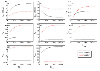
Figure 2: The averaged total kinetic energy per nucleon $E_{kin}$ (a), total potential energy per nucleon $E_{pot}$ (b), the multiplicity information entropy $H$ (c), the multiplicities of the emitted neutrons $N_{n}$ (d), protons $N_{p}$ (e), charged particles $N_{cp}$ (f) and intermediate mass fragment $N_{imf}$ (g), the heaviest fragment mass $A_{max}$ (h) over the ’spin’-exchange step as a function of step at $\rho_{f}$ = 0.38 $\rho_{0}$ and T = 3 or 6 MeV in the framework of I-LGM. The symbols are illustrated in the right bottom.

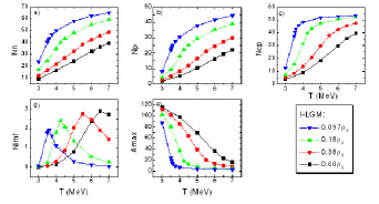
Figure 3: Average multiplicity of the emitted neutrons $N_{n}$ (a), protons $N_{p}$ (b), charged particles $N_{cp}$ (c) and intermediate mass fragment $N_{imf}$ (d), the mean mass of the largest fragment $A_{max}$ (e) as a function of temperature in different ‘freeze-out’ density in the framework of I-LGM. The symbols are illustrated in the right bottom.

III.1 I-LGM in different ’freeze-out’ densities

Figure 3 shows that the mean multiplicities of emitted neutrons, protons, CP and IMF and the mean mass for the largest fragment evolve with temperature at different ‘freeze-out’ densities in the I-LGM calculation. Here IMF is defined as 3 $\leq$ Z $\leq$ 20. At a fixed ‘freeze-out’ density, average neutron multiplicity ( $N_{n}$ ), proton multiplicity ( $N_{p}$ ), charged particle multiplicity ($N_{cp}$ ) and the mean mass for the largest fragment ( $A_{max}$ ) display monotonous increase or decrease with temperature as expected. But the multiplicity ( $N_{imf}$ )ofIMFshowsariseandfallwith temperature [27, 28], when the system probably crosses the phase transition boundary. With decreasing ‘freeze-out’ density, $N_{p}$, $N_{n}$, $N_{cp}$ and $A_{max}$ increase, since larger space separation among nucleons at smaller ‘freeze-out’ density makes the clusters less bound and therefore the sizes of free clusters decrease and then the cluster multiplicities increase. The situation of $N_{imf}$ is slightly complicated, i.e. it increases with the decrease of ‘freeze-out’ density in the lower temperature branch contrary to the higher temperature branch.

It seems difficult to discover the possibility of phase transition of nuclei if we only see these mean quantities as shown above ( $N_{imf}$ is an exception ). However, when we focus on their slopes to temperature (figure 4), sharp changes are observed at nearly the same temperature at each fixed ‘freeze-out’ density, for instance, 3.5 MeV at 0.097$\rho_{0}$, 4MeV at 0.18$\rho_{0}$, 5MeV at 0.38$\rho_{0}$ and 6 MeV at 0.60$\rho_{0}$. At such a transition point, (1) the multiplicities of emitted clusters increase rapidly and after that the emission rate slows down; and (2) the decrease in the largest fragment size reaches a valley for such a finite system. Physically, the largest fragment is simply related to the order parameter $\rho_{l}-\rho_{g}$ (the difference of density in nuclear ‘liquid’ and ‘gas’ phases). In infinite matter, the infinite cluster exists only on the ‘liquid’ side of the critical point. In finite matter, the largest cluster is present on both sides of the phase transition point. In this calculation, a valley for the slope of $A_{max}$ to temperature may correspond to a sudden disappearance of infinite cluster (‘bulk liquid’) near the phase transition temperature. It is not the occasional production of such waves of the slopes; it should reflect the onset of phase transition there. This idea is supported by surveying the other phase transition observables, such as the effective power law parameter $\rho_{f}$rom the mass or charge distribution of fragment and the information entropy $H$ of event multiplicity distribution [19]. $H$ can be expressed as

$$H=-\sum_{i\in Event}p_{i}\cdot ln(p_{i})$$ (7)

where $p_{i}$ is defined as the event-normalized total multiplicity probability and $\sum_{i\in Event}p_{i}$ = 1. Figure 5 depicts these results. The minima of $\tau$ and the maxima of $H$ appear around respective phase transition temperatures at different values of ‘freeze-out’ density, i.e. about 3.5 MeV at 0.097$\rho_{0}$ , 4–4.25 MeV at 0.18$\rho_{0}$, 5–5.5 MeV at 0.38$\rho_{0}$ and 6–6.5 MeV at 0.60$\rho_{0}$. These temperatures are consistent with those extracted from the choppy position of the above slopes. It indicates that the above slopes (emission rate) can be taken as a probe of a liquid–gas phase transition of nuclei.

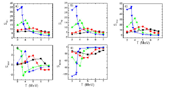
Figure 4: Same as in figure 3, but for their slopes with temperture. The symbols are the same as in figure 3.

Furthermore, the largest fluctuations of cluster multiplicities are found around the phase transition point in the same calculation. Figure 6 illustrates that RMS width ( $\sigma$ ) of the multiplicity distributions of neutrons, protons, CP and IMF, and the distribution of the largest fragment masses. These variances generally show peaks at the same phase transition temperatures as those extracted from the above observables for each fixed ‘freeze-out’ density. Note that the fluctuation of $A_{max}$ is related to the compressibility of the system. These features are also consistent with one of the phase transition behaviours, i.e. the largest fluctuation at the phase transition point exists [29]. This fluctuation represents an internal feature of the disassembling system, not a numerical fluctuation.

Another way to characterize the fluctuation is the method of the conditional moments introduced by Campi [30]. The normalized second moment $S_{2}$ in each event is defined as

$$S_{2}=\frac{\sum_{A_{i}\neq A_{max}}{A_{i}}^{2}\cdot n_{i}(A_{i})}{\sum_{A_{i}\neq A_{max}}{A_{i}}\cdot n_{i}(A_{i})}$$ (8)

where $n_{i}$ is the multiplicity of cluster mass $A_{i}$ , and the summation is over all clusters in an event except the heaviest one which corresponds to the bulk liquid in an infinite system. For example, we show the 1000-event Campi scatter plots ( ln($A_{max}$) versus ln($S_{2}$) ) as a function of temperature at a fixed density of 0.38$\rho_{0}$ in figure 7. Actually, the plots clearly illustrate the evolution of the disassembling mechanism with temperature. At lower temperatures, only the under-critical (liquid phase) branch with a negative slope of ln($A_{max}$) versus ln($S_{2}$) exists while at higher temperature, only the super-critical (gas phase) branch with a positive slope of ln($A_{max}$) versus ln($S_{2}$) appears. However, both the branches (the liquid–gas phase coexistence region) meet closely around 5.5 MeV, which indicates the onset of the liquid–gas phase transition [28, 30, 31]. Similar behaviour shows for the calculation at 0.097$\rho_{0}$ ,0.18$\rho_{0}$ and 0.60$\rho_{0}$ at their respective phase transition temperature.

We point out that the ‘freeze-out’ density-dependent phase transition temperature, extracting from $\tau$ and $S_{2}$ , was also observed in a previous study [32]. Similar to water, the temperature of liquid–gas phase transition decreases with pressure. In the nuclear case, the decrease in ‘freeze-out’ density is similar to the decrease in the internal pressure inside nuclei, hence it leads to decrease in transition temperature. But this $\rho_{f}$-dependent phenomenon vanishes when excitation energy is used as a variable in the LGM [33]. In other words, the excitation energy has perhaps a good correspondence with the critical temperature because of only one critical point and hence only one critical temperature for a system.

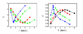
Figure 5: The effective power law parameter $\tau$ of cluster mass distribution (left) and the information entropy $H$ (right) as a function of temperature in different ‘freeze-out’ densities in the framework of I-LGM. The symbols are the same as in figure 3.

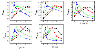
Figure 6: Temperature-dependent RMS widths ( $\sigma$ ) of the distributions of $N_{n}$ (a), $N_{p}$ (b), $N_{cp}$ (c), $N_{imf}$ (d) and $A_{max}$ (e) in different ‘freeze-out’ densities in the framework of I-LGM. The symbols are the same as in figure 3.

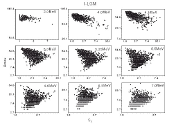
Figure 7: Campi scattering plots for I-LGM at 0.38$\rho_{0}$ . excitation energy has perhaps a good correspondence with the critical temperature because of only one critical point and hence only one critical temperature for a system.

III.2 Roles of Coulomb force: comparison of I-LGM and I-CMD in fixed ’freeze-out’ density

Considering the absence of long-range Coulomb force in the LGM, we adopt the CMD to investigate the Coulomb effect and check the features of cluster emission and its relation to phase transition behaviour. To this end, first we make a comparison for the results of I-CMD with Coulomb or without Coulomb and those of I-LGM at a certain fixed ‘freeze-out’ density, namely 0.38$\rho_{0}$ . Second, we present the results of all these observables in the frame of I-CMD with Coulomb at four different ‘freeze-out’ densities to check cluster emission and its relation to the phase transition behaviour in next subsection.

Figure 8 shows that $N_{p}$ , $N_{n}$ , $N_{cp}$ , $N_{imf}$ and $A_{max}$ change with temperature in different calculation cases, i.e. I-CMD with Coulomb or without Coulomb and I-LGM (see the meaning of the symbols in the figure.). The multiplicities of clusters and the largest fragment mass are close to each other between I-LGM and I-CMD with Coulomb except for the multiplicities of neutrons and protons, illustrating that the I-LGM is, in general, a good tool to describe the fragmentation if Coulomb interaction can be ignored. When Coulomb interaction is switched on, $N_{p}$ , $N_{cp}$ and $N_{imf}$ increase due to the repulsive role among protons while $A_{max}$ decreases. Meanwhile, $N_{n}$ does not change because of no Coulomb interaction. $N_{imf}$ also shows a rise and fall with temperature in the I-CMD cases. Coulomb force makes the turning temperature of $N_{imf}$ smaller due to long-range repulsion.

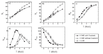
Figure 8: Same as in figure 3, but for comparison between different calculations: I-LGM (open circles), I-CMD without Coulomb interaction (open squares) and I-CMD with Coulomb force (solid squares). The ‘freeze-out’ density of system is 0.38$\rho_{0}$ .

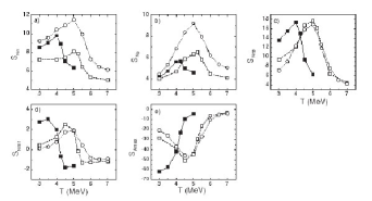
Figure 9: Same as in figure 4, but for comparison between different calculations: I-LGM (open circles), I-CMD without Coulomb interaction (open squares) and I-CMD with Coulomb force (solid squares). The ‘freeze-out’ density of system is 0.38$\rho_{0}$ .

The slopes of multiplicities of emitted clusters and of mean mass of the largest fragment are plotted as a function of temperature in case of I-CMD in figure 9. The definite peaks of slopes are found as in the I-LGM case. The corresponding temperature at the peaks is located about 4 MeV in the I-CMD case with the Coulomb interaction and about 5 MeV in the I-CMD case without the Coulomb interaction. This turning temperature also reflects the onset of phase transition there. If we investigate $\tau$ and $H$ (figure 10), we find that there are a minima of $\tau$ and the maxima of $H$ around phase transition temperatures, i.e. about 4–4.25 MeV for I-CMD with the Coulomb, around 5 MeV for I-CMD without the Coulomb and around 5.5 MeV for I-LGM respectively.

Finally, the RMS widths of the multiplicity distributions of the clusters and of the largest fragment mass are checked in the I-CMD case in figure 11. The widths of the multiplicity distributions of neutrons and protons tend to be saturated at higher temperature, while those for CP, IMF and $A_{max}$ demonstrate peaks at a certain fixed temperature, i.e. around 4 MeV for the case I-CMD with the Coulomb, 5 MeV for the case of I-CMD without the Coulomb, which is similar to the I-LGM case. These turning temperatures are also consistent with the phase transition temperature as shown in figures 8–10 in the I-CMD cases.

Overall, Coulomb interaction plays a notable role in favour of fragment production and reduces the temperature of the phase transition. When the system is small, the Coulomb interaction is not expected to be important and I-LGM could be a good tool to treat nuclear disassembly. But for large nuclear systems, the neglect of the Coulomb force in LGM is rather serious handicap. In this background, first, we made a suitable selection for the molecular dynamics interaction potential and then got good agreement between the I-LGM and I-CMD without the Coulomb. Thanks to this agreement, we treated the nuclear disassembly more realistically with switching on of the Coulomb interaction in the frame of I-CMD afterwards.

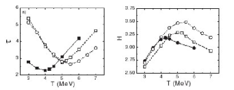
Figure 10: Same as in figure 5, but for comparison between different calculations: I-LGM (open circles), I-CMD without Coulomb interaction (open squares) and I-CMD with Coulomb force (solid squares). The ‘freeze-out’ density of system is 0.38$\rho_{0}$ .

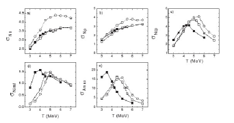
Figure 11: Same as in figure 6, but for comparison between different calculations: I-LGM (open circles), I-CMD without Coulomb interaction (open squares) and I-CMD with Coulomb force (solid squares). The ‘freeze-out’ density of system is 0.38$\rho_{0}$ .

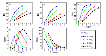
Figure 12: Same as in figure 3 but in the case of I-CMD with Coulomb.

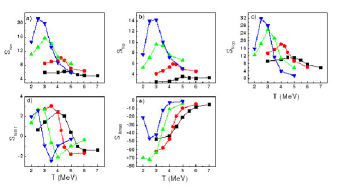
Figure 13: Same as in figure 4 but in the case of I-CMD with Coulomb. without the Coulomb. Thanks to this agreement, we treated the nuclear disassembly more realistically with switching on of the Coulomb interaction in the frame of I-CMD afterwards.

III.3 I-CMD in different ’freeze-out’ densities

Similar to the I-LGM cases, we also study the cluster emission in I-CMD in a wide range of ‘freeze-out’ density, namely, 0.097$\rho_{0}$ ,0.18$\rho_{0}$ ,0.38$\rho_{0}$ and 0.60$\rho_{0}$ to check phase transition behaviour.

In order to compare it with the I-LGM case, similar figures are plotted in figures 12–15 and compared to figures 3–6. Figure 12 shows that the mean multiplicities of emitted neutrons, protons, CP, IMF and $A_{max}$ evolve with temperature at different ‘freeze-out’ densities in the I-CMD calculation with the Coulomb. Their emission rates or slopes and RMS width with temperature are depicted in figures 13 and 15. The effective power-law parameter of fragment distribution $\tau$ and multiplicity information entropy $H$ is plotted in figure 14. All these figures show the same behaviours as the I-LGM case, i.e. cluster emission rate and their fluctuation can provide us with the temperature of liquid–gas phase transition, namely around 3, 3.5, 4.5, 5 MeV at $\rho_{f}$ = 0.097$\rho_{0}$ ,0.18$\rho_{0}$ ,0.38$\rho_{0}$ and 0.60$\rho_{0}$ respectively.

Similarly, the Campi’s scattering plots indicate the onset of liquid–gas phase transition around the respective transition temperatures. Figure 16 shows an example for I-CMD with the Coulomb. Clearly, phase coexistence takes place around 4.25 MeV. Overall, these phase transition temperatures are consistent with those extracted from the choppy position of the slopes of figure 13. Again, the largest fluctuation simultaneously appears at the point of phase transition.

Overall, the phase transition temperature seems to rely on some ingredients, such as the ‘freeze-out’ density (or pressure), the model and its interaction potential, but the rule that emission rate and fluctuation of cluster multiplicity can be taken as a probe of phase transition has not changed.

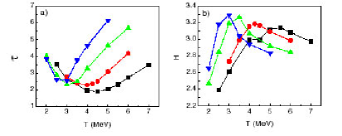
Figure 14: Same as in figure 5 but in the case of I-CMD with Coulomb.

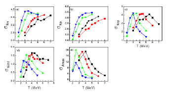
Figure 15: Same as in figure 6 but in the case of I-CMD with Coulomb.

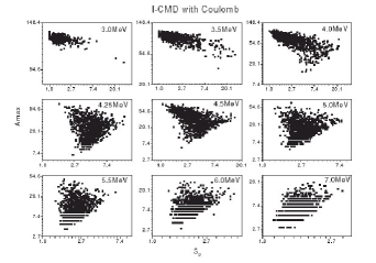
Figure 16: Same as in figure 7, but for the I-CMD with Coulomb case at 0.38$\rho_{0}$ .

IV Conclusions

In conclusion, the features of the emissions of LP, CP, IMF and MAX are investigated in a wide range of ‘freeze-out’ density for a medium size nucleus ${}^{129}Xe$ in the frameworks of I-LGM and I-CMD model. $N_{n}$, $N_{p}$, $N_{cp}$ and $A_{max}$ show monotonous increase or decrease while $N_{imf}$ shows rise and fall with temperature. Slopes of these observables versus temperature go through extrema at the same temperature where the largest fluctuation of cluster multiplicity distributions is observed. This temperature is consistent with the phase transition temperature extracted from the extreme values of effective power law parameter $\tau$ and information entropy $H$ as well as Campi scatter plots. It gives an indication that the cluster emission rate can be taken as a probe of the phase transition of nuclei and furthermore, the largest fluctuation is simultaneously accompanied when the onset of phase transition occurs. In addition, the systematic comparison of I-LGM and I-CMD shows that LGM is a good tool to study nuclear disassembly when the system is not large where the Coulomb interaction can be ignored. But for large nuclear systems, I-CMD should be used to treat the nuclear dissociation and phase transition due to the importance of the Coulmb interaction. In light of this study, we think that the experimental study of cluster emission is rather meaningful, especially in measuring the excitation function of the multiplicities, their slopes and variances, from which some signals of phase transition could be found.