Fano theory for hadronic resonances:
the rho meson and the pionic continuum

Abstract

We develop a model-independent analysis of hadronic scattering data in the resonance region, where the resonance shape follows from the matrix elements of a Hamiltonian. We investigate the rho meson in the tau decay. We demonstrate that the rho meson resonance in the two-pion decay of the tau lepton is described well through the coupling of a bare rho meson to the two-pion and the four-pion continuum. Furthermore, this four-pion continuum corresponds with the data of the four-pion decay channel of the $\tau^{-}$ at energies up to $1.1$ GeV.

I Introduction

The most obvious unstable hadronic states, or resonances, are single absorption peaks in the $\pi N$ scattering data in a particular channel, with a Breit-Wigner, or Lorentz, shape, where the width is related to the coupling to mainly pionic decay channels. However, resonances generally have distorted shapes due to the presence of other resonances or thresholds of competing channels. Their shape might look nothing like the Breit-Wigner shape that is often used to fit the data, and the position of the peak might shift through inter-resonance and resonance-continuum interactions. The extraction of single resonances from complex scattering data is still strongly model dependent VDL .

Today, baryons are no longer tied to $\pi N$ scattering, but are also observed in other experiments, such as $\gamma N$ scattering. They are particles in their own right, which can be probed with different experiments. However, hadrons are not elementary particles. QCD was discovered as the underlying microscopic field theory of composite hadrons. In principle hadrons are bound states of quarks, but deriving their properties directly from QCD has proven difficult. Therefore, the interest in hadronic resonances has been extended from basic resonance parameters, such as the mass and the width, to microscopic properties that can test the quality of a wide range of microscopic models of hadrons. Although most models reproduce the mass spectrum with a reasonable accuracy, microscopic properties, such as charge radii and magnetic moments, and branching ratios of decays are currently under investigation.

Furthermore, quark models allow for states, hybrids or exotics, that do not consist of three quarks, or simple quark-anti-quark pairs. However, to extract a clear signal for these states from experiment is a formidable task. Therefore, it is important to understand the conventional hadronic states and their coupling to possible exotic states better.

Since the first analysis of hadronic resonances there have been many theoretical developments. Quantum field theory has replaced quantum mechanics as the fundamental theory for small-scale physics, and renormalization is an unfortunate, but integral part of a modern approach based on local interactions. In hadron physics the issue of handling divergences and renormalization is often by-passed by introducing form factors or vertex functions. Vertex form factors which smear the interactions and make further regularization superfluous fail to have universal applicability; each experiment within a particular energy range is explained with a model which has its own form factors. Global models that fit the world data do a good job in the energy range of the world data, but these models would not necessarily lead to good predictions for new results at higher energies.

The local interactions in field theory seem essential to maintain relativistic covariance, and, although models with vertex form factors can reproduce the data well with a limited number of parameters, they are tied to a particular experiment, a particular energy range, and a particular set of channels, and they say very little general about a particular hadronic state. Moreover, a different set of vertex form factors might do just as well.

Furthermore, there are bounds and constraints, such as unitarity and analyticity, on the models that describe scattering. They were put on a firm footing by study of the analytical properties of the S-matrix, and are incorporated in quantum field theory. However, since hadrons are not elementary particles, there is no fundamental field theory, with a small number of parameters, that describes all of hadron dynamics. Model field theories of hadron physics serve to bring order in the complexity, to restrict the model space, and to implement constraints from symmetries.

Separate from the choice of the model hadronic field theory, the theory of resonances has unfortunately not kept pace with the developments in field theory in general. Consistency requires that the imaginary part of the mass is of an unstable particle follows from a microscopic model that links the particle with its decay channels. Some formal developments have been made MS59 ; Zwa63 ; however, in practice the models underlying the resonance shapes that describe actual data, which can be very complicated, are in essence the same as those of thirty years ago BW52 ; tola . These models aim to locate the resonance poles, but gives very little other information that can constrain models of hadron interactions. Microscopic properties of hadrons remain hidden in the data.

Some theoretical progress has been made. For example, resonances have been studied and renormalization is handled in chiral perturbation theory KKW . However, the typical energy of hadronic resonances is too high and lies beyond the region of applicability of chiral perturbation theory. At these energies the chiral symmetry is not important, and other features, such as form factors or a large number of low-energy parameters dominate the fit to the data. The hadronic Lagrangian is not restricted by chiral symmetry at these energies, and many constants need to be fitted to the data.

In most cases, attempts to describe medium-energy hadronic physics from an underlying field theory start with a chiral Lagrangian which is augmented with additional constraints. For example, one important, but approximate conservation law in medium-energy hadronic physics, which has been utilized, follows from vector meson dominance. This suggests there is a universal hadronic current by which the photon and the rho meson couple to all hadrons HLS . Furthermore, the large $N_{c}$ limit has some implications for amplitudes, which can restrict the $SU(3)_{f}$ chiral Lagrangian so that it has predictive power Lut00 . In more traditional chiral Lagrangian approaches unitarity has been used to improve the predictions beyond the original range of applicability oller . Finally, from a more traditional hadronic few-body dynamics point of view, a consistent implementation of covariance can extend the range of validity and restrict the model dependence Pic01 . For most of these approaches, scales and form factors still need to be introduced. Furthermore, the models are more designed to test the assumptions made, than to extract universal quantities from a wide range of scattering data. In all these approaches hadrons enter as the elementary fields. Independently, within the Dyson-Schwinger framework, there are investigations on the way to use their rho meson Bethe-Salpeter results in baryon and meson form factors tandy , where the composite nature of hadrons in terms of quarks is resolved.

Our aims are much simpler; we would like to determine universal quantities, like the matrix elements of a Hamiltonian, directly and consistently from the data. Consistent tools for the analysis of resonances that satisfy unitarity, analyticity are developed. They meet a microscopic model for hadrons halfway in terms of matrix elements and bare masses. The divergences that arise from the local interactions are renormalized, and the only parameters present are a few coupling constants and bare masses. Simple field-theoretical results, such as the bubble summation for a single channel are reproduced. The method is much more versatile, and this versatility is paramount. The coupled channel data should yield an Hamiltonian with the same asymptotic states first. If there is an important inelastic cross section, the only models that can be trusted are those which explicitly take into account these channels. Possible candidates for resonances can be added and their effects on the data studied. It is not a matter of explaining a particular set of data, but it is important to have independent verifications of resonances in independent experiments.

Any other input is considered part of a microscopic model, and should be kept in its simplest form. The approach does not hinge on a particular approximation, but solely on one condition. Any approximation should be made at the level of the Hamiltonian and it should maintain Hermiticity. The Hamiltonian is a good starting point and end point of such tools: formulate a model in terms of a Hamiltonian, and fix the matrix elements with the data. Unitarity, analyticity, and other constraints on the data are automatically fulfilled within this approach.

This method for analysis of hadronic resonances is designed for the case of a strong coupling between continua and multiple resonance states. This paper is the first step in developing a set of tools for a fully unitary approach to coupled-channel scattering problems, which is under investigation at the moment. Furthermore, it establishes contact with the local field theories that should describe these systems, and renormalization is handled.

In most studies resonances are fitted with Breit-Wigner resonance shapes, however, resonances have often more complicated shapes. In atomic theory there is a wide range of methods developed that describe resonances or auto-ionization profiles. In hadronic physics the interaction is stronger. The resonances have generally a larger width, and therefore more complicated shapes as they interact with other resonances and the asymtotic states. The method used here is an adaption of a method developed by Fano in the 1960’s.

Fano developed Fan61 ; Cow82 ; BR97 an analysis for atomic resonances by writing down a general Hamiltonian for such systems. This Hamiltonian can be diagonalised exactly, thereby yielding direct relations between scattering data and the parameters of the Hamiltonian. It is based on the separation of the problem into two parts: the continuum, characterized by the energy of the asymptotic states in a particular channel, and resonances, which in the absence of a continuum are discrete eigenstates, such as, the states that would follow from a constituent quark model, large $N_{c}$ approximation, or a quenched lattice calculation.

The continuum should be considered an eigenstate of the decoupled system as well. The wave function could be deformed at the origin with respect to the non-interacting wave function due to direct continuum-continuum interaction as would occur in field theory. In this case the continuum can be composite; with asymptotic states without fixed particle numbers, as we will see in section IV where we discuss the rho meson as an example. By splitting the problem in two and expressing it in the eigenstates of the sub-problems many matrix elements are zero due to orthogonality of the eigenstates of the sub-problems.

As a first example we analyze the rho meson resonance in the tau decay. The resonance shape dominates the hadronic decay of the tau lepton into two pions. We choose to describe this problem with a bare rho which couples to a two-pion state. The energy dependence of the coupling can be modeled by a chiral Lagrangian. To extend this simple model, there are two main avenues: introduce a more complicated energy dependence, motivated by some microscopic model, or introduce the next state that is important, which is the four-pion state (with a threshold at $558$ MeV). For the data it is clear that the four-pion decay of the tau lepton dominates the two-pion decay above 1 GeV. The effects of four-pion states are hard to handle in chiral perturbation theory, since this involves at least a three-loop diagram and many intermediate states, such as $\omega\pi$, $\rho\rho$, $\pi\pi\rho$, and $a_{0}\pi$ mesons BR69 . However, we will see that a simple four-pion state does precisely what is needed: it corrects the high-energy part of the two-pion decay, and gives a quantitative prediction of the four-pion decay. In the Hamiltonian approach the details of of the rho four-pion coupling cannot be resolved with present-day data. The two effective coupling constants; the two-pion and the four-pion decay of the rho meson are sufficient to describe the hadronic tau lepton below $1.1$ GeV. Above this energy there are many channels which can only be distinguished by looking at invariant masses of subsystems in multi-pion states to which most of these hadronic states decay. At the moment only the three-pion decay of the intermediate omega meson has a clear signal Eck , mainly because of the narrow width of the omega.

Many theoretical studies of the rho meson focus on combining vector meson dominance (VMD) Sak60 with chiral symmetry. In these models the photon couples to most hadrons through a universal conserved vector current (CVC). The microscopic foundation of this current, and its underlying symmetry, is poorly understood, and a hidden local symmetry (HLS) is postulated HLS . This symmetry mixes the photon with the rho meson. The additional knowledge resulting from this assumption has led to a reasonable understanding of the shape of the rho meson due to coupling with the two-pion continuum.

However, since chiral perturbation theory focusses on low-energy behavior, the predicted higher energy behavior does not agree with the data, because the higher order derivative couplings violate unitarity at intermediate energies. Therefore, the high-energy part of the rho resonance fails the data completely. Improved HLS models unitarize previous results, and somewhat improve agreement. We, on the other hand, find the correct high-energy behavior by simply including the four-pion continuum.

In the next section, we will develop the general theory of resonances given a Hamiltonian with a number of discrete states and a continuum. In Section III we show that the matrix elements that appear in the Hamiltonian can be related to Feynman diagrams. For a first application to hadronic resonances we apply the method to the rho meson in Section IV. In Section V we present the results, and the final section we discuss future applications and improvements of this method.

II Theory

Let us first consider a general Hamiltonian which couples a continuum to a set of discrete states that are orthogonal with respect to each other. Many systems can be cast in this form (it does not allow for continuum-continuum interactions, which is a topic of current investigations). The Hamiltonian has the general form:

$$H = \sum_{i=1}^{k}|i\rangle\epsilon_{i}\langle i|+\int d\Delta\ |\Delta\rangle\Delta\langle\Delta|$$ (1)

$$+\sum_{i=1}^{k}\int W_{i}(\Delta)d\Delta\ \left(|\Delta\rangle e^{-i\phi_{i}(\Delta)}\langle i|\ +\ |i\rangle e^{i\phi_{i}(\Delta)}\langle\Delta|\right)\ \ ,$$

where $\epsilon_{i}=\sqrt{{\bf p}^{2}+M_{i}^{2}}$ with ${\bf p}$ the momentum of the system, and $M_{i}$ is the mass of the discrete, bare state $i$. The continuum state $|\Delta\rangle$ is labeled with its energy $\Delta$. The coupling is parametrized with the unknown coupling functions $W_{i}$ and phases $\phi_{i}$. In practice, such Hamiltonian are restricted to a particular channel, with a given partial wave, charge, and other conserved quantum numbers, which we therefore omit from the start.

All the integrals are principal value integrals, additional terms that arise from the singularities will be taken in account explicitly, rather than implicitly in a particular pole or $i\epsilon$ prescription, which places the pole at a particular side of the contour integration. The latter is used in scattering theory, where the pole part is associated with open channels, or asymptotic, states. Within an eigenfunction interpretation, we do not necessarily interpret singular parts of the eigenstate with out-states, they could be in-states as well, or, if the interaction is strong, mix with the resonance state. This information is carried in the occupation numbers $\alpha_{i}$ and $\beta$, which are normalized to unity, even for a singular functional dependence of the spectroscopic strength $\beta$ on the energy.

The eigenstates $|\omega\rangle$ with the continuous energy $\omega$ of the Hamiltonian can be expressed as:

$$|\omega\rangle=\int d\Delta\beta(\omega,\Delta)|\Delta\rangle+\sum_{i=1}^{k}\alpha_{i}(\omega)|i\rangle\ \ .$$ (2)

where $\alpha_{i}$’s are the occupation numbers of the discrete state, and $\beta$ is the spectroscopic amplitude, or occupation density, of the continuum states. Substituting this into the Hamiltonian, Eq. ((1)), we can express $\beta(\omega,\Delta)$ in terms of the $\alpha$’s:

$$\beta(\omega,\Delta)=\left(\frac{1}{\omega-\Delta}+z(\omega)\delta(\omega-\Delta)\right)\sum_{i=1}^{k}\alpha_{i}(\omega)W_{i}(\Delta)e^{-i\phi_{i}(\Delta)}\ \ .$$ (3)

where $z(\omega)$ can be any regular function to be determined later. $z(\omega)(\omega-\Delta)\delta(\omega-\Delta)$ vanishes. Substituting $\beta$ back into the second equation of the Hamiltonian, Eq. (1), yields:

$$(\omega-\epsilon){\bf\alpha}(\omega) = \pi{\cal F}(\omega)\cdot{\bf\alpha}(\omega)+z(\omega){\bf F}(\omega)\cdot{\bf\alpha}(\omega)\ \ ,$$ (4)

where $(\omega-\epsilon)$ is a diagonal matrix with entries $\omega-\epsilon_{i}$. The hermitian matrix ${\bf F}$, and its Hilbert transform ${\cal F}$ necessary for the consistency condition on $z(\omega)$ are defined:

$$F_{ji}(\xi) = W_{i}(\xi)W_{j}(\xi)e^{i(\phi_{j}(\xi)-\phi_{i}(\xi))}\ \ ,$$ (5)

$${\cal F}_{ji}(\eta) = \frac{1}{\pi}\int d\xi\frac{F_{ij}(\xi)}{\eta-\xi}\ \ .$$ (6)

Eq. (4) is multiplied from the left by:

$${\bf W}^{\dagger}(\omega)\cdot\left((\omega-\epsilon)-\pi{\cal F}(\omega)\right)^{-1}\ \ ,$$ (7)

where the vector ${\bf W}^{\dagger}(\omega)=(W_{1}(\omega)e^{-i\phi_{1}(\omega)},W_{2}(\omega)e^{-i\phi_{2}(\omega)},\cdots,W_{k}(\omega)e^{-i\phi_{k}(\omega)})$. The whole expression contains a common factor ${\bf W}^{\dagger}(\omega)\cdot\alpha(\omega)$, which can be divided out, which yields a closed form expression for $z(\omega)$:

$$z(\omega)=\left({\bf W}^{\dagger}(\omega)\cdot\left((\omega-\epsilon)-\pi{\cal F}(\omega)\right)^{-1}\cdot{\bf W}(\omega)\right)^{-1}\ \ .$$ (8)

At this point it is important to realize the significance of $z(\omega)$ above: it is the projected resolvent $((\omega-\epsilon)-\pi{\cal F}(\omega))^{-1}$ of the discrete spectrum, perturbed through the coupling with the continuum. Given that ${\cal F}$ is hermitian, the matrix $(\epsilon-\pi{\cal F})$ will have a discrete spectrum $\omega_{1},\omega_{2},\cdots,\omega_{k}$,

$$\Omega=\left(\begin{array}[]{cccc}\omega_{1}&&&\cr&\omega_{2}&&\cr&&\ddots&\cr&&&\omega_{k}\end{array}\right)=U^{\dagger}(\omega)\cdot\left(\epsilon-\pi{\cal F}(\omega)\right)\cdot U(\omega)\ \ .$$ (9)

In order to simplify the results, it is convenient to work in the basis of the true spectrum of the discrete system. In this case the inverse, that appears in Eq. (8), is trivial. We perform the substitutions:

$$\alpha(\omega) = U\cdot{\bf a}(\omega)\ \ ,$$ (10)

$${\bf W}(\omega) = U\cdot{\bf V}(\omega)\ \ ,$$ (11)

and likewise for the hermitian conjugates.

The normalization of the state $|\omega\rangle$ yields:

$$\langle\omega^{\prime}|\omega\rangle = \alpha^{\dagger}(\omega^{\prime})\cdot\alpha(\omega)$$

$$+\alpha^{\dagger}(\omega^{\prime})\cdot\frac{z(\omega^{\prime}){\bf W}(\omega^{\prime}){\bf W}^{\dagger}(\omega^{\prime})-\pi{\cal F}(\omega^{\prime})}{\omega^{\prime}-\omega}\cdot\alpha(\omega)$$

$$-\alpha^{\dagger}(\omega^{\prime})\cdot\frac{z(\omega){\bf W}(\omega){\bf W}^{\dagger}(\omega)-\pi{\cal F}(\omega)}{\omega^{\prime}-\omega}\cdot\alpha(\omega)$$

$$+(\pi^{2}+z^{2}(\omega))\delta(\omega-\omega^{\prime})\alpha^{\dagger}(\omega^{\prime})\cdot{\bf W}(\omega^{\prime}){\bf W}^{\dagger}(\omega)\cdot\alpha(\omega)\ \ ,$$

where the $\pi^{2}$ contribution results from the pole term of the product of the two principal value singularities in the spectroscopic densities $\beta$. If we substitute the new variables, a and V, it is easy to see that the first three terms cancel each other. The state $|\omega\rangle$ is an eigenstate by construction and:

$$\langle\omega^{\prime}|\omega\rangle=(\pi^{2}+z^{2}(\omega))\delta(\omega-\omega^{\prime})\alpha^{\dagger}(\omega^{\prime})\cdot{\bf W}(\omega^{\prime}){\bf W}^{\dagger}(\omega)\cdot\alpha(\omega)\ \ .$$ (13)

The probability of finding the system in the discrete state $|i\rangle$, given it was in the discrete state $|j\rangle=|\psi(t=0)\rangle$ is:

$$\langle i|\psi(t)\rangle=\int d\omega\ \alpha_{i}(\omega)\alpha_{j}^{\ast}(\omega)e^{-i\omega t}\ \ ,$$ (14)

where the occupation numbers are given by:

$$\alpha_{i}(\omega)=\frac{W_{i}(\omega)e^{-i\phi_{i}(\omega)}}{{\bf W}^{\dagger}{\bf W}\left[z(\omega)+i\pi\right]}\ \ ,$$ (15)

and we have chosen a convenient phase. At the position of a resonance $\omega=\omega_{j}$, $z(\omega_{j})$ vanishes, however, this is not necessarily the resonance maximum, as the coupling function depends on the energy. If the coupling function is a constant, a single resonance shape reduces to a Breit-Wigner form:

$$\alpha_{j}(\omega)=\frac{W_{j}}{(\omega-\omega_{j})+i\pi W_{j}^{2}}\ \ .$$ (16)

Likewise, the phase shift follows from the inspection of Eq. (3) for the spectral density of the continuum state. The principal value singularity yields the scattering wave function proportional to $-\pi\sin(k(\omega)+\delta_{l})$, while the delta function yields the scattering wave function proportional to $\sin(k(\omega)+\delta_{l}+\frac{\pi}{2})$. Therefore, their relative strength $\pi/z(\omega)$ determines the effect of the coupling to the discrete states to the phase shift $\delta_{r}$, which yields

$$\delta_{r}=-\arctan\frac{\pi}{z(\omega)}\ \ .$$ (17)

Clearly, once the eigenstate is known, in terms of the occupation numbers $\alpha_{i}$ of the discrete states and the occupation number $\beta$ of the continuum, at every energy we can determine any quantity we like. The decay of a state is given by the probability of finding the system in that state, Eq. (14). In a scattering process, the incoming state must be projected on the continuum part of the eigenstate, and the scattering continuum state can be reached subsequently via one of the discrete states. Transition amplitudes are therefore proportional to $W_{j}\alpha_{j}$. For a single channel the $T$-matrix is:

$$T=\frac{1}{z(\omega)+i\pi}\ \ ,$$ (18)

which preserves unitarity.

III Coupling functions

Figure 1: The two diagrams from which the coupling functions $W$ and $W_{2}$, between the discrete state and the continuum, is derived.

The masses $M_{i}$ and the coupling functions $W_{i}$ are to be determined by other means. We assume that the masses follow from some QCD or constituent-quark based model. Although, the coupling functions; the pion-hadron interaction, could in principle be determined by the same means, in practice that turned out to be a formidable task. Therefore, we turn to Lagrangians with explicit pions and chiral symmetry for the coupling functions BR69 . The easiest connection is made midway. Although the meaning of the Green’s function, or resolvent, is different in the study of eigenstates, which is stationary, and the study of scattering, which is dynamical, the actual mathematical form is the same. At many levels one can find relations between expressions in scattering theory and stationary eigenvalue problems. We choose the equivalence that is most convenient to us, which is the equivalence of the one-particle self-energy. With chiral Lagrangians we can determine the one-particle irreducible self-energy correction $\Sigma$ of hadrons due to coupling to the pion field, which is given in terms of Feynman diagrams. We can equate this with the real part of energy shift due to the coupling of the $i$-th discrete state with the continuum $\pi{\cal F}_{ii}$ in the Fano theory, which also yields the real part of the self-energy due to the coupling with the continuum:

$$\int_{PV}d\Delta\frac{W_{i}^{2}(\Delta)}{\omega-\Delta}\equiv\Sigma_{i}(\omega)=\frac{1}{2\omega}{\rm Re}\int d^{4n}k\ I(k)\ \ ,$$ (19)

where $I$ is the integrand of the truncated Feynman self-energy diagram $\Gamma$ for the bare hadron $i$. Hence $W_{i}^{2}$ is the phase-space of the continuum times the appropriate factors:

$$W_{i}^{2}(\omega)=\frac{\pi}{2\omega}{\rm Im}\int d^{4n}k\ I(k)\ \ ,$$ (20)

where $\omega$ is the sum of the free energies of the particles in the continuum state, which, in a Feynman diagram with energy conservation at the vertices, equals the total incoming energy. Similarly, in the right-hand side of Eq. (19) we can recognize the corresponding Goldstone diagram BR86 .

This connection between the coupling function $W$ and the imaginary part of the Feynman diagram guarantees that the tree-level and bubble-sum results in this approach and with Feynman diagrams are the same. However, the Hamiltonian description does not automatically include the backward, or anti-particle, contributions, since these are related to separate states. These states must be added explicitly. The major advantage is that the resulting linear eigenvalue equation in the energy can be solved exactly, even in the case of multiple resonances and multiple decay channels. In the language of Feynman diagrams this statement corresponds to the simultaneous bubble sum of the different intermediate states.

Figure 2: The two backward, or Z diagrams. The inclusion of these two states in the coupling functions restores covariance, but does not affect the shape of the resonance, only coupling constants change slightly.

For the rho meson, analyzed below, we included the anti-particle states, that is, we combined $\rho\to\pi\pi\to\rho$ with the $\rho\to\rho\rho\bar{\pi}\bar{\pi}\to\rho$ process and $\rho\to\pi\pi\pi\pi\to\rho$ with $\rho\to\rho\rho\bar{\pi}\bar{\pi}\bar{\pi}\bar{\pi}\to\rho$. (See Fig. 2.) Although this restores covariance it has little effect on the actual resonance shape, since the threshold of the $\rho\rho\pi\pi$ state is already above $1800$ MeV. The calculation of the self-energy simplifies for the rho meson; the functions depend on $s=\omega^{2},\Delta^{2}$ only, since the forward and the backward contributions combine. Schematically:

$$\int d\Delta\frac{f(\Delta^{2})}{\omega-\Delta}+\int d\Delta\frac{f(\Delta^{2})}{\omega-(2\omega+\Delta)}=\int d\Delta^{2}\frac{f(\Delta^{2})}{\omega^{2}-\Delta^{2}}\ \ .$$ (21)

The self-energy Eq. (19) is highly divergent for many pionic problems. We will use on-shell subtraction as our renormalization procedure, which requires implicit counterterms such that the masses $M_{i}$ and the wave function normalization $\langle i|j\rangle=\delta_{ij}$ remain unaltered. In practice the wave-function renormalization means a unit residue of the resonance pole. Below we discuss the rho meson, and show explicitly how these problems are handled.

IV The rho meson

The rho meson plays an important role in photon-hadron interactions at intermediate energies. It seems that the photon couples to hadrons mainly via the isovector-vector rho meson, which in its turn, couples to a universal hadronic current via a coupling constant $g$. We see the rho meson mainly through its decay to two pions. So in order to describe the physical rho meson, we assume a discrete state $|\rho\rangle$ at rest, which couples to the two-pion continuum $|\pi\pi(\Delta)\rangle$ with energy $\Delta$. We have the following matrix elements:

$$\langle\rho|H|\rho\rangle = M\ \ ,$$ (22)

$$|\langle\rho|H|\pi\pi(\Delta)\rangle|^{2} = \frac{g^{2}(\Delta^{2}-4m_{\pi}^{2})^{\frac{3}{2}}\theta(\Delta-2m_{\pi})}{48\pi\Delta}=W^{2}(\Delta)\ \ ,$$ (23)

$$\langle\pi\pi(\Delta^{\prime})|H|\pi\pi(\Delta)\rangle = \Delta\delta(\Delta-\Delta^{\prime})\ \ ,$$ (24)

where the coupling function follows from the interaction term $g\vec{\rho}^{\mu}\cdot[\vec{\pi}\times\partial_{\mu}\vec{\pi}]$ in the chiral Lagrangian, and the vectors are in the isospin space. In practice this particular coupling is only important for the right threshold behavior, for large energies the results are dominated by the phase space. For the moment we will assume that there is no self-interaction in the two-pion continuum, therefore the coupling function $W$ follows the phase space. The explicit unitarity of the approach and the on-shell renormalization lead to the correct large energy behavior.

In the future we will investigate the effect of the continuum-continuum interaction on the results. We also include the next contribution to the physical rho, which, considering the possible states in this channel and their energies, must be the four-pion state, with a threshold at $558$ MeV. From an energy of about $1$ GeV there are many other intermediate decay channels important, e.g.: $\pi^{6}$, $\omega\pi$, $\rho\pi^{2}$ and $a_{0}\pi$ between $900$ MeV and $1.5$ GeV BR69 . They are to be taken in account if one wants to analyze rho decay at energies above $1$ GeV. For example, the $\pi\omega$ system has a threshold ($921$ MeV) close enough to the $\rho$ mass ($770$ MeV) to yield contributions that do not simply follow the four-pion phase space. However, we leave this to future investigations. Although channels open at a slightly lower energy than $1.1$ GeV, their effect is not strong at threshold due to the low-energy behavior manifest in the derivative couplings of the chiral Lagrangian.

From the chiral Lagrangian there are many intermediate states that lead to the four-pion state from the discrete rho, however, all these states are highly virtual, so we can approximate the coupling between the discrete rho and the four-pion state with a single derivative coupling. (See Fig. 1.) This yields a complicated integral, equivalent to a three-loop calculation in Feynman perturbation theory. Ignoring these correlations in the four-pion state, the additional matrix elements are well-approximated by:

$$|\langle\rho|H|\pi\pi\pi\pi(\Delta)\rangle|^{2} = \frac{g_{2}^{2}(\Delta^{2}-16m_{\pi}^{2})^{\frac{9}{2}}\theta(\Delta-4m_{\pi})}{M^{5}\Delta^{3}}\equiv W_{2}^{2}(\Delta)\ \ ,$$ (25)

$$\langle\pi\pi\pi\pi(\Delta^{\prime})|H|\pi\pi\pi\pi(\Delta)\rangle = \Delta\delta(\Delta-\Delta^{\prime})\ \ .$$ (26)

From semi-analytical three-loop calculations Lig00 one can see that the approximation for $W_{2}$ is reasonable, and the eigenstates of the complete system turn out to be stable under small variations in the coupling function $W_{2}$. The continuum is composite. It contains a two-pion and a four-pion fraction to the ratio $W/W_{2}$. We did not allow a direct coupling between them, so they mix with ratios proportional to the coupling strengths to the discrete state $|\rho\rangle$.

The real parts, from Eq. (6), are divergent integrals, as expected for local interactions. Therefore we need to regularize the results and state how we determine the finite parts. In hadronic physics renormalization has to be pragmatic, since most theories for hadronic physics are not renormalizable; there is no fixed set of parameters, masses and coupling constants that can re-absorb all the divergences by a proper redefinition. Therefore, at any order or scale a number of observables are needed to fix the unknown finite renormalizations of the system. In principle a lot of fine-tuning, to fit theory to experiment, can be done here. However, we take the view that this fine-tuning means fitting the short and medium range physics, which should be done with a proper microscopic theory of hadrons. The bare rho is the result of miscroscopic interaction that should incorporate the short range effects of pions. Therefore all the finite renormalizations are chosen such that the contributions vanishes at the rho mass $M$. This is a choice, but it separates analysis of scattering data from any model assumptions. If some additional knowledge about the structure of the rho meson exists, it should end up in the coupling function. This is important to make the analysis based on the Hamiltonian scale independent, since scale dependence implies model dependence.

For this purpose we use on-shell renormalization; subtracting the low-order divergent terms in Taylor expansion in $(\omega^{2}-M^{2})$ of the self-energy ${\cal F}$. Note that since we have included the anti-particle diagrams, Eq. (21), our self-energy ${\cal F}$ is a function of $s=\omega^{2}$ rather than $\omega$, hence the expansion is in $(\omega^{2}-M^{2})$ rather than $(\omega-M)$. Odd terms are absent and do not require renormalization.

The two-pion coupling function leads to the ordinary mass and wave-function renormalization $c_{0}$ and $c_{1}(\omega^{2}-M^{2})$. The four-pion coupling function requires subtractions $c^{(2)}_{0}$, $c^{(2)}_{1}(\omega^{2}-M^{2})$, $c^{(2)}_{2}(\omega^{2}-M^{2})^{2}$, and $c^{(2)}_{3}(\omega^{2}-M^{2})^{3}$, which are set identical to the same divergent terms in ${\cal F}_{\pi^{4}}$:

$$c^{(2)}_{n}=\frac{1}{n!}\left.\frac{\partial^{n}{\cal F}_{\pi^{4}}(\omega^{2})}{\partial(\omega^{2})^{n}}\right|_{\omega=M}\ \ .$$ (27)

The effects of the self-energy are small over the whole range of the rho resonance shape, from the two-pion threshold to $1.2$ GeV, which yields effects of the order of a couple of percent.

Since the finite renormalization is model independent there are only two parameters to fit the data. These are the two coupling constants $g$ and $g_{2}$, which yield the strength of the coupling between the bare rho and the two-pion continuum and the four-pion continuum respectively. Since the two decay channels are both open at these energies, There are also have two independent measurements of these two coupling constants; namely, the two-pion decay and the four-pion decay.

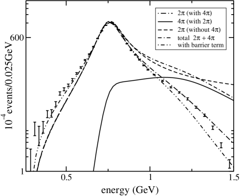
Figure 3: The Fano calculation compared with the $\tau^{-}$ decay data from the CLEO collaboration CLEO . There are three cases: the two-pion results without four-pion contributions (long dashed), the results for the two-pion (dot-dashed) and four-pion (solid) continua and their sum (dot-dash-dashed), and the change in the two-pion decay of the latter if an artificial barrier term CLEO is introduced, and coupling constants refitted (dot-dot-dashed).

V Results

The hadronic tau decay at the CLEO experiment is dominated by the rho meson in the intermediate state. The initial tau lepton decays into a neutrino and a W-boson. Subsequently the W-boson produces a hadronic state via the standard model Lagrangian $Wq\bar{q}$ vertex. After all the electroweak structure has been resolved, the hadronic part of the decay is dominated by the rho meson resonance at energies between the hadronic decay threshold, which is the two-pion threshold and about $1$ GeV when the $\omega\pi$ channel is open and the first of many other decay channels start to compete.

The experimental data from CLEO CLEO is represented in Fig. 3, where the number of events, freed from electroweak dependences, is plotted as a function of the invariant mass of the two-pion system. The same figure summarizes our analysis. If the bare rho state couples only to a two-pion continuum, the high-energy tail of the resonance peak is grossly overestimated. If the four-pion continuum is included, the two-pion decay channel is suppressed at higher energies, in favor of four-pion decay (they cross just above $1$ GeV). The total pionic decay comes again to the same value as the original two-pion-only result, however, the shape of the inclusive resonance peak at these higher energies is different.

For completeness, a fit with a barrier term is also included BW52 , as was used in the data analysis CLEO . The barrier term has its origin in nuclear quantum mechanics and relates the amplitude of the asymptotic wave function with the inner part in the nuclear potential. These two parts are matched at the Coulomb barrier through which an escaping radiative-decay particle tunnels. The momentum dependence of this matching is reflected in the barrier term. There is no field-theoretical analogue of the barrier term. It reproduces the right low-energy behavior; however, within our analysis, which has only two parameters, we pay for the rather artificial low-energy improvement with a failure at higher energies. The position and the slope of the four-pion decay events compare well with both the OPAL OPAL and the CLEO CLEO plots for four-pion events.

Comparing the resonance shape with the results from our Hamiltonian and fitting the two coupling constants $g$ and $g_{2}$ to hadronic decay of the $\tau^{-}$ we find a number of results. First, from the fit of the $\pi\pi$ decay of the $\rho$-meson, we find a coupling constant $g_{2}\approx 0.2$ to the four-pion state, which agrees well, without any fitting, with the actual four-pion data OPAL between threshold ($0.558$ GeV) and $1.1$ GeV. Beyond $1.1$ GeV we expect other contributions, which decay to four pions, like $\omega\pi$, to be important.

Second, if we consider the pion as an elementary particle, the initial state, as generated by the electroweak process, will be the discrete rho state. From the actual two-pion data which falls of as $\omega^{-2}$ for high energies we infer that there is no direct coupling to the two-pion continuum, as this would lead to large amplitudes for large energies. Corrections to this assumption of the pion as an asymptotic but pointlike particle, which follows from combining Fano theory with the chiral Lagrangian, could improve the low-energy fit but would fail to descibe the data at higher energies KKW .

Third, the presence of the four-pion continuum changes the two-pion coupling constant. It is interesting to notice that the coupling constants have to be adjusted if additional, non-interacting channels are included. The competition between decay modes generates a simple, but effective final-state interaction.

Fourth, the real part, after the on-shell renormalization, yields a negligible effect. Since, with on-shell renormalization, the real part vanishes when the energy equals the rho mass, the value of the real part is small in the neighborhood of this value.

Finally, we are unable to get a very good fit to the data near threshold, within the model. There have been several suggestions to improve the results KKW ; HLS , based on chiral symmetry. These all use a direct electroweak-pion-pion coupling, which violates unitarity for large energies. Physically there are two explanations for the deviations, within our scheme. Firstly, the coupling between the electroweak state and the bare rho could have a momentum dependence, due to, for example, a pionic, or $q\bar{q}$ quark, rho wave function. This should be visible in an additional quenching of the electroweak decay modes at the energies just above the two-pion threshold. Secondly, the electroweakly produced initial state could contain a two-pion state, but only at low energies. It is hard to motivate this from a underlying local theory. This is equivalent to unitarized hidden local symmetry (HLS) models HLS .

VI Discussion

For the problem of the rho meson studied here we did not require the full machinery of the Fano theory. For example, there is only one discrete state in the system. In the case of a neutral rho meson the mixing with the $\omega$ meson could be taken into account explicitly and unitarily.

For the moment it has been more important to show that the two-pion and the four-pion continua describe the rho resonance well, where the four-pion continuum results in two independent observations: its effect on the two-pion decay, and a direct measurement of the four-pion decay of the rho meson. All this can be discussed at the level of restricted Hamiltonians. These Hamiltonians contain given states and continua which are expected to dominate the results (in this case a composite continuum consisting of two- and four-pion states in the rho channel, and the bare rho state). The fact that no further approximation is required allows one to draw definite conclusions, whether these states and continua actually dominate the physics in a certain channel and at a certain energy, or other degrees of freedom are necessary. In this case the data between $0.6$ GeV and $1.1$ GeV is well-described by these degrees of freedom.

The Fano theory allows one to go further in particle numbers and complexity than other methods. Complex states can be build up hierarchically by admixing states in their expected order, similar to angular momentum coupling schemes in atomic physics. The only aspect not handled in Fano theory is the particle number conserving interaction between continua as occurs in field theory. Instead of these self-interacting states we assume the states to be eigenstates already, with the only noticeable effect a deformation of the phase space in $W$, with respect to the free-particles phase space, due to the changed dispersion relation $\omega({\bf k})\not=\sum_{i}\sqrt{{\bf k}^{2}+m_{i}^{2}}$, to be calculated separately or approximated by the free result.

In the future we plan to apply this method to baryonic resonances, for which a lot of new data is becoming available from recent JLAB experiments. In these experiments the problems with data analysis are more stringent due to the rich spectra and the higher energies VDL . We will also investigate the way in which to extend Fano theory to allow for continuum-continuum interactions.

References

- (1) T. P. Vrana, S. A. Dytman, and T. S. H. Lee, Phys. Rept. 328, 181 (2000).
- (2) P. T. Matthews and A. Salam, Phys. Rev. 115, 1079 (1959).
- (3) D. Zwanziger, Phys. Rev. 131, 2818 (1963).
- (4) J. M. Blatt and V. F. Weisskopf, Theoretical nuclear physics, (New York, Wiley, 1952); H. Feshbach, Theoretical nuclear physics, (New York, Wiley, 1991).
- (5) S. Jadach, J. H. Kühn, and Z. Was, Comput. Phys. Commun. 64, 275 (1991); 70, 69 (1992); 76, 361 (1993).
- (6) F. Klingl, N. Kaiser, and W. Weise, Z. Phys. A 356, 193 (1996).
- (7) H. B. O’Connell et al., Nucl. Phys. A 623, 559 (1997); M. Benayoun et al., Z. Phys. C 72, 221 (1996).
- (8) M. F. Lutz and E. E. Kolomeitsev, Found. Phys. 31, 1671 (2001).
- (9) J. A. Oller and E. Oset, Phys. Rev. D 60, 074023 (1999).
- (10) M. A. Pichowsky, A. Szczepaniak, and J. T. Londergan, Phys. Rev. D 64, 036009 (2001).
- (11) P. Tandy (private communication); P. Maris and P. C. Tandy, Phys. Rev. C 60, 055214 (1999).
- (12) U. Fano, Phys. Rev. 124, 1866 (1961).
- (13) R. D. Cowan, The Theory of Atomic Structure and Spectra, (University of California Press, 1982).
- (14) S. M. Barnett and P. M. Radmore, Methods in theoretical quantum optics, (Oxford Press, Oxford, 1997).
- (15) L. Banyai and V. Rittenberg, Phys. Rev. 184, 1903 (1969).
- (16) E. von Toerne (private communication); K. W. Edward et al. (CLEO), Phys. Rev. D 61, 072003 (2000);
- (17) J. Sakurai, Ann. Phys. (N.Y.) 11, 1 (1960).
- (18) J. P. Blaizot and G. Ripka, Quantum Theory of Finite Systems, (MIT Press, Cambridge (MA), 1986).
- (19) N. E. Ligterink, Phys. Rev. D 61, 105010 (2000).
- (20) S. Anderson et al. (CLEO), Phys. Rev. D 61, 112002 (2000).
- (21) K. Ackerstaff et al. (OPAL), Eur. Phys. J. C 7 571 (1999)