Building light nuclei from neutrons, protons, and pions

Abstract

In these lectures I first explain, in a rather basic fashion, the construction of effective field theories. I then discuss some recent developments in the application of such theories to two- and three-nucleon systems.

1 Introduction: what is an effective theory?

An effective theory is a systematic approximation to some underlying dynamics (which may be known or unknown) that is valid in some specified regime. An effective theory is not a model, since its systematic character means that, in principle, predictions of arbitrary accuracy may be made. However, if this is to be true then a small parameter, such as the $\alpha$ of quantum electrodynamics, must govern the systematic approximation scheme. As we shall see here, in many modern effective theories the expansion parameter is a ratio of two physical scales. For instance, in effective theories of supersymmetric physics “beyond the standard model” the ratio would be of $p$ or $m$, the momentum or mass of a standard model particle, to $M_{\mathrm{S}USY}$. In an effective theory for finite-proton-size effects in the hydrogen atom the small parameter would be $r_{\mathrm{p}}$, the proton size, divided by $r_{\mathrm{b}}$, the Bohr radius. The smallness of this parameter is then indicative of the domain of validity of the effective theory (ET). In this sense effective theories, like revolutions, carry the seeds of their own destruction, since the failure of the expansion to converge is a signal to the user that he or she is pushing the theory beyond its limits. Within the radius of convergence of the ET the ET “works” because of the following fundamental tenet:

Phenomena at low energies (or long wavelength) cannot probe details of the high-energy (or short-distance) structure of particles.

I suspect that most physicists subscribe to this tenet: indeed, if the tenet were not true, then physics (other than calculations using a “theory of everything”) would be impossible.

In this first section I will begin by discussing the basic ideas of effective theories using a few simple examples from undergraduate physics. In this way we will move from classical effective theories, to classical effective field theories (EFTs), to quantum effective field theories. Of course, to understand the latter one must be able to compute quantum-field-theoretic loop graphs, so this requires a little more education than the standard undergraduate curriculum contains—at least the undergraduate curriculum at American Universities! Nevertheless, I will attempt to present the work at a level that is understandable by someone who has completed a first course on quantum field theory, but has not necessarily yet studied the theory of regularization and renormalization.

In Section 2 I will begin to focus on the nucleon-nucleon (NN) system. This will first necessitate some definitions of terms, notation, and so forth. I then move on to discuss the special issues stemming from the presence of shallow bound states in the NN problem. After displaying one solution to this difficulty, I will define and employ an effective field theory which takes into account the presence of shallow bound states, but other than this only contains neutrons and protons as dynamical degrees of freedom. I will give examples of the success of this EFT, known as ${\mathrm{E}FT}({\pi\hskip-6.00006pt/})$, in computing (very-)low-energy electromagnetic observables in the NN system.

The extension of this work to the three-body problem raises some intriguing problems of renormalization. I will attempt to elucidate these in Section 3, where I draw on the work of Bedaque, Hammer, and van Kolck, to show how, after some thought and interesting discoveries, ${\mathrm{E}FT}({\pi\hskip-6.00006pt/})$ can be applied to the NNN problem.

Finally, in Section 4 I give a brief tour of results in an effective field theory with pions. The effective field theory of QCD in which nucleons and pions are the degrees of freedom is chiral perturbation theory ($\chi$PT). We were fortunate to have one of the founders of $\chi$PT, and indeed a pioneer in the field of EFTs, lecturing at this school. Prof. Leutwyler’s lectures in this volume should be read in conjunction with the material presented here. Indeed, this article should be regarded as little more than light reading on the subject of nuclear EFTs. It is very far from being a thorough review on the topic. The reader who wishes to study the subject in detail should consult the reviews Ref. [1, 2] which contain much more information than does this manuscript. These two reviews also contain full references to the original literature, a job I have not tackled in any systematic way here.

1.1 Some very simple effective theories

1.1.1 Gravity for $h<R$

One of the simplest effective theories I know is one that is learned by high-school physics students. It concerns the standard formula for the gravitational potential-energy difference of an object of mass $m$ which is raised a height $h$ above the Earth’s surface:

$$\Delta U=mgh,$$ (1)

where $g$ is the acceleration due to gravity

Of course from Newton’s Law of Universal Gravitation (itself an effective theory, valid in the limit of small space-time curvature), we have

$$\Delta U=-{{GMm}\over{r_{\mathrm{f}}}}+{{GMm}\over{r_{\mathrm{i}}}},$$ (2)

for an object whose distance from the Earth’s centre is initially $r_{\mathrm{i}}$ and finally $r_{\mathrm{f}}$. Now, if we write

$$r_{\mathrm{f}}=r_{\mathrm{i}}+h,$$ (3)

and assume that $r_{\mathrm{i}}\approx R$, the radius of the Earth, then

$$\Delta U=m{{GM}\over{R^{2}}}{R\over{R+h}}h.$$ (4)

Identifying $\frac{GM}{R^{2}}=g$ we see that Eq. (1) is only the first term in a series, which converges as long as $h/R<1$:

$$\Delta U=mgh\left(1-\frac{h}{R}+\frac{h^{2}}{R^{2}}+\ldots\right).$$ (5)

If we try to apply this theory to a satellite in geosynchronous orbit ($h\gg R$) the series will not converge. But for the space shuttle ($h\sim$ a few hundred km) this series should converge fairly rapidly. Equation (1) is the first term in the effective theory expansion (5) for the gravitational potential energy, with that ET being valid for $h<R$.

1.1.2 Effective theories in the hydrogen atom

Presumably, the hydrogen atom is ultimately described in terms of string theory, or some other fundamental theory of physics. Nevertheless, to very good precision, we can use quantum electrodynamics (QED) as an effective theory to compute its spectrum. The reason why we can ignore corrections to QED from physics at the Planck scale when calculating the hydrogen-atom spectrum will become clear below.

In the case of the hydrogen atom there is an effective theory for QED that is valid up to corrections suppressed by one power of $\alpha=e^{2}/(4\pi)$, the fine-structure constant. That effective theory is known as the Schrödinger equation with the Coulomb potential. The radial wave function $u_{nl}(r)$ obeys the differential equation : 5

$$-{1\over{2m_{\mathrm{e}}}}{{d^{2}u_{nl}}\over{dr^{2}}}+{{l(l+1)}\over r^{2}}u_{nl}(r)-{\alpha\over r}u_{nl}(r)=E_{n}u_{nl}(r).$$ (6)

The solution, for the lowest-energy eigenstate ($n=1$; $l=0$) is, of course:

$$u_{10}(r)={\mathcal{}N}\,\exp(-\alpha m_{\mathrm{e}}r)={\mathcal{}N}\,\exp(-r/r_{\mathrm{b}})\,,$$ (7)

where $r_{\mathrm{b}}=(\alpha m_{\mathrm{e}})^{-1}\approx(4\mbox{ keV})^{-1}\approx 0.5~{}\AA$, and $\mathcal{}N$ is determined by the normalization condition. The corresponding eigenvalue is

$$E_{10}=-{1\over 2m_{\mathrm{e}}}\left({1\over r_{\mathrm{b}}}\right)^{2}.$$ (8)

The Bohr radius, $r_{\mathrm{b}}$, sets the scale for most phenomena associated with the electron in the Hydrogen atom. In particular, the typical momentum of the electron is $\sim 1/r_{\mathrm{b}}$, which means that relativistic corrections to the Schrödinger equation are suppressed by $(m_{\mathrm{e}}r_{\mathrm{b}})^{-2}=\alpha^{2}$, thereby validating the non-relativistic treatment. Note that if we were discussing muonic hydrogen the energy and distance scales would be very different, since $r_{\mathrm{b}}^{\mu}\approx\frac{1}{200}r_{\mathrm{b}}^{e}$.

The Bohr radius is large compared to the size of the proton, $r_{\mathrm{p}}$, and also compared to the scale of internal structure of the electron. One sense in which the electron has internal structure is that it is dressed by virtual photons. In fact, the Lamb shift is, in fact, just such an electron-structure effect, so “finite-electron-size” effects must be considered if very accurate results are desired. If we for the moment ignore the electron’s internal structure and consider only the internal structure of the proton we would replace the Coulomb potential $-\alpha/r$, by the potential generated by an extended proton:

$$V({\mathbf{r}})=-{e^{2}\over 4\pi}\int\,{{\rho({\mathbf{r}}^{\prime}){\mathrm{d}}^{3}r^{\prime}}\over{|{\mathbf{r}}-{\mathbf{r}}^{\prime}|}},$$ (9)

with $\rho({\mathbf{r}}^{\prime})$ the local electric charge density of the proton at the point ${\mathbf{r}}^{\prime}$. Now we make a multipole expansion, in order to obtain:

$$V({\mathbf{r}})=-{e^{2}\over 4\pi r}\sum_{n=0}^{\infty}\left({r_{\mathrm{p}}\over r}\right)^{n}\int\,{\mathrm{d}}^{3}r^{\prime}\,\rho({\mathbf{r}}^{\prime})P_{n}(\hat{r}\cdot\hat{r}^{\prime})\left({r^{\prime}\over r_{\mathrm{p}}}\right)^{n}~{}~{}~{}\mbox{for $r>r_{\mathrm{p}}$,}$$ (10)

with $P_{n}$ the nth Legendre polynomial. Here, $\rho(\mathbf{r}^{\prime})$ only has support for $r^{\prime}<r_{\mathrm{p}}$, and so the integrals are all numbers of order one. Since the solution of the differential equation (6) is mainly sensitive to $r\sim r_{\mathrm{b}}$, the expansion parameter here is $r_{\mathrm{p}}/r_{\mathrm{b}}\sim 1~{}\AA/1~{}{\mathrm{f}m}$, and so this series converges rapidly, with it entirely permissible to evaluate the corrections for the finite size of the proton in perturbation theory. Nevertheless, an accurate computation requires inclusion of the term of order $(r_{\mathrm{p}}/r_{\mathrm{b}})^{2}$ in this expansion.

In fact, this term of $O((r_{\mathrm{p}}/r_{\mathrm{b}})^{2})$ is the first correction due to finite-size effects in Eq. (6). This is easily seen from Eq. (10), since the coefficient of the term of $O(r_{\mathrm{p}}/r_{\mathrm{b}})$ is zero, as long as the proton’s charge distribution is even under parity. Thus consideration of the scales in the problem alone would lead us to grossly overestimate the magnitude of the finite-size effect. It is the combination of scales and symmetry that leads to an accurate estimate of the magnitude of the effects neglected by assuming that the proton is point-like in Eq. (6). These two principles:

• a ratio of scales generating an expansion parameter,

• symmetries constraining the types of corrections that can appear,

inform the construction of most effective theories.

1.2 Building a (classical) effective theory: the scattering of light from atoms

Next I want to discuss an example of ET-construction which first appeared in print in the effective field theory lecture notes of Kaplan [3]. These lecture notes are an excellent introduction to EFT, and this example provides a great demonstration of ET construction. Here I have reworked some of the notation, but the basic idea is as in Ref. [3].

Consider the scattering of low-energy light from an atom. The question we must answer is: What is the Hamiltonian that describes the interaction of the atom with the electromagnetic field of the incoming light? To do this, we first consider the scales in the problem: the energy of the electromagnetic field, $\omega$ is assumed small compared to the spacing of the atomic levels, $\Delta E$, and the inverse size of the atom. We will assume in turn that all of these scales are much smaller than the mass of the atom. Using $r_{\mathrm{b}}$ to estimate $\Delta E$ we have the following hierarchy of scales:

$$\omega\ll\Delta E\sim{1\over m_{\mathrm{e}}r_{\mathrm{b}}^{2}}\ll{1\over r_{\mathrm{b}}}\ll M_{\mathrm{a}tom}.$$ (11)

Meanwhile the symmetries of the theory will be electromagnetic gauge invariance [$U(1)_{\mathrm{e}m}$], rotational invariance, and Hermitian conjugation/Time reversal. These symmetries constrain the types of terms that we can write in our Hamiltonian. Firstly, the constraint of gauge invariance suggests that it is wise to construct $H_{\mathrm{a}tom}$ out of the quantities ${\mathbf{E}}$ and ${\mathbf{B}}$, rather than using the four-vector potential $A_{\mu}$. Then, secondly, rotational invariance suggests that we employ quantities such as ${\mathbf{E}}^{2}$ and ${\mathbf{E}}\cdot{\mathbf{B}}$ in $H_{\mathrm{a}tom}$. However, ${\mathbf{E}}\cdot{\mathbf{B}}$ is odd under time reversal, and so we cannot write down a term proportional to it in $H_{\mathrm{a}tom}$. Meanwhile, terms such as ${\mathbf{\nabla}}\cdot{\mathbf{B}}$, and ${\nabla}\times{\mathbf{E}}$ may be included in $H_{\mathrm{a}tom}$, but then can be eliminated from the Hamiltonian using the field equations for the electromagnetic field in the region around the atom:

$$\nabla\cdot{\mathbf{E}}=0; \nabla\cdot{\mathbf{B}}=0;$$ (12)

$$\nabla\times{\mathbf{E}}=0; \nabla\times{\mathbf{B}}=0.$$ (13)

This leaves us with:

$$H_{\mathrm{a}tom}=a_{1}{\mathbf{B}}^{2}+a_{2}{\mathbf{E}}^{2}+a_{3}(\partial_{0}{\mathbf{B}}^{2})+a_{4}(\partial_{0}{\mathbf{E}}^{2})+a_{5}({\mathbf{E}}\cdot{\mathbf{B}})^{2}+\ldots$$ (14)

In spite of our cleverness in constraining the terms that may appear, we are still left with infinitely many operators that can contribute to $H_{\mathrm{a}tom}$. How are we to organize all of these contributions?

Interlude: naive dimensional analysis

The answer lies in the scale hierarchy established in Eq. (11), together with a simple technique known as naive dimensional analysis (NDA). This works as follows: consider, for instance, the operator ${\mathbf{B}}^{2}$. Counting powers of energy/momentum we see that it carries four powers of energy, which we write as:

$$[{\mathbf{B}}^{2}]=4.$$ (15)

However, $H_{\mathrm{a}tom}$ must have dimensions of energy. It follows that $a_{1}$ and $a_{2}$ must each carry three negative powers of energy/momentum:

$$[a_{1}]=[a_{2}]=-3,$$ (16)

that is to say:

$$a_{1},a_{2}={1\over(\mbox{some energy scale})^{3}}.$$ (17)

Now we ask what energy scales are present in the problem and so might appear in the denominator here. The photon energy $\omega$ cannot appear in the denominator since the scale that occurs there should refer to a property of the atom. Any of the scales $r_{0}^{-1}$, $\Delta E$, or $M_{\mathrm{a}tom}$ could be involved though. The most conservative estimate would be that:

$$a_{1},a_{2}\sim{1\over(\Delta E)^{3}}.$$ (18)

However, very low-energy photons cannot probe the quantum level structure of the atom: they should interact with the entire atom in an essentially classical way. Thus, $\Delta E$ cannot occur in the denominator of this lowest-dimensional term in the Hamiltonian, and so we deduce that $a_{1}$ and $a_{2}$ must scale with $r_{0}$, i. e.:

$$a_{1},a_{2}\sim r_{0}^{3},$$ (19)

where the $\sim$ usually indicates that the coefficient here could be a 3 or a 1/3 (or a -3 or a -1/3) but will generally be a number of order one . $a_{1}$ and $a_{2}$ are in fact proportional to the electric and magnetic polarizabilities of the atom [4].

Meanwhile, the operators multiplying the coefficients $a_{3}$ and $a_{4}$ have dimension 5. Thus, $[a_{3}]=[a_{4}]=-4$, and so $a_{3}$ and $a_{4}$ carry one more energy-scale downstairs as compared to $a_{1}$ and $a_{2}$. Conservatively, we assign the scaling:

$$a_{3},a_{4}\sim{r_{0}^{3}\over\Delta E}.$$ (20)

Similar estimates can be made for the other terms in $H_{\mathrm{a}tom}$. The key point is that since ${\mathbf{B}}^{2}$ and ${\mathbf{E}}^{2}$ are the lowest dimension operators allowed by the symmetries and not already constrained by field equations, they will give the dominant effect in $H_{\mathrm{a}tom}$ for low-energy photons. Any higher-order effects will be suppressed by at least $\omega/\Delta E$, i. e.:

$$H_{\mathrm{a}tom}=r_{0}^{3}\left[\tilde{a_{1}}{\mathbf{B}}^{2}+\tilde{a_{2}}{\mathbf{E}}^{2}+O\left({\omega\over\Delta E}\right)\right],$$ (21)

where $\tilde{a_{1}}$ and $\tilde{a_{2}}$ are now dimensionless numbers. It is straightforward to turn this result into a prediction for the photon-atom cross section. Since $[\sigma]=-2$ and the cross section results from squaring the quantum-mechanical amplitude arising from the Hamiltonian (21) we discover that

$$\sigma\sim\omega^{4}r_{0}^{6}$$1+O${\omega\over\Delta E}$$$,$$ (22)

where the $\sim$ disguises the hard work needed to figure out all the factors of 2, $\pi$ and so forth that really go into deriving $\sigma$! The strong dependence of $\sigma$ on $\omega$ is, of course, the reason the sky is blue—as pointed out in Ref. [3] or in Ref. [5], where the constant of proportionality in Eq. (22) is worked out in detail!

1.3 A classical effective field theory: Fermi electroweak theory

Equation (21) is an effective expression for the classical Hamiltonian that is valid at long wavelength, or equivalently, for low-energy electromagnetic fields. In general effective field theories are derived for low energies, although this need not be the case.

A canonical example of a low-energy effective field theory is Fermi’s electroweak theory. This is an effective field theory that can be used to compute, say, low-energy electron-neutrino scattering. The only particles explicitly appearing in this theory are electrons and neutrinos. By contrast, in the standard model, the electrons and neutrinos interact by the exchange of W and Z bosons. If we wish to compute the scattering of neutrinos from electrons we could compute the full standard model amplitude for diagrams such as Fig. 1 [6]:

$${\mathcal{}A}=\left({-{\mathrm{i}}g\over 2\cos\theta_{\mathrm{W}}}\right)$\bar{\nu}P_{\mathrm{L}}\gamma_{\mu}\nu${{\mathrm{i}}\over q^{2}-M_{\mathrm{Z}}^{2}}\left({-{\mathrm{i}}g\over 2\cos\theta_{\mathrm{W}}}\right)$\bar{e}\gamma^{\mu}Qe$;$$ (23)

with:

$$P_{\mathrm{L},R} = \frac{1}{2}(1\mp\gamma_{5});$$ (24)

$$Q = (-1+2\sin^{2}\theta_{\mathrm{W}})P_{\mathrm{L}}+2\sin^{2}\theta_{\mathrm{W}}P_{\mathrm{R}}.$$ (25)

and $q=p^{\prime}-p$ being the change in momentum of the neutrino. Relating $q^{2}$ to laboratory quantities, we see that:

$$q^{2}=-4E_{\mathrm{l}ab}E^{\prime}_{\mathrm{l}ab}\sin^{2}${\theta_{\mathrm{l}ab}\over 2}$,$$ (26)

where $E_{\mathrm{l}ab}$ ($E^{\prime}_{\mathrm{l}ab}$) and $\theta_{\mathrm{l}ab}$ are the initial (final) energy and scattering angle of the neutrino in the lab. system. So, if $E_{\mathrm{l}ab}\ll M_{\mathrm{Z}}$, then we can expand the Z-propagator in Taylor series. The leading term in this series is then:

$${\mathcal{}A}={\mathrm{i}}\sqrt{2}G_{\mathrm{F}}$\bar{\nu}P_{\mathrm{L}}\gamma_{\mu}\nu$$\bar{e}\gamma^{\mu}Qe$,$$ (27)

with:

$$G_{\mathrm{F}}={g^{2}\over 4\sqrt{2}\cos^{2}\theta_{\mathrm{W}}}{1\over M_{\mathrm{Z}}^{2}}={g^{2}\over 4\sqrt{2}M_{\mathrm{W}}^{2}}.$$ (28)

The effective Lagrangian that generates the amplitude (27) is:

$${\mathcal{}L}_{\mathrm{F}ermi}=G_{\mathrm{F}}\sqrt{2}$\bar{\nu}\gamma_{\mu}P_{\mathrm{L}}\nu$$\bar{e}\gamma^{\mu}Qe$.$$ (29)

This is the amplitude written down by Fermi many years ago for beta-decay and associated processes. The argument given here for deriving $G$ from the underlying theory goes under the rubric “tree-level matching”.

Fig. 1. : A Feynman diagram for neutrino-electron scattering via exchange of a Z⁰ particle.

Note that while the range of the neutrino-electron interaction (23) is of order $1/M_{\mathrm{Z}}$, the interaction (29) is of zero range. All four fields in the Lagrangian (29) are to be evaluated at the same space-time point, $x$. This approximation is sensible provided that the neutrino’s energy is such that its Compton wavelength is much longer than $1/M_{\mathrm{Z}}$. In this circumstance the standard model Lagrangian may be approximated by a Lagrangian in which the electrons and neutrinos interact only when they are right on top of each other, since then the neutrino cannot resolve the finite range of its interaction with the electron. A more accurate approximation to the standard-model may be obtained by expanding the Z-boson propagator in powers of $q^{2}/M_{\mathrm{Z}}^{2}$. These higher-order pieces of the Fermi electroweak theory Lagrangian will give rise to operators of a higher dimension than the operator (29), which has dimension:

$$2[\nu]+2[e]=6.$$ (30)

This is a crucial point, since the operator $\bar{\nu}\nu\bar{e}e$ is the lowest-dimension one we can construct out of the four lepton fields. This means that even if we knew nothing about electroweak interactions, we would still expect an interaction like (29) to be the leading term describing low-energy electron-neutrino scattering. Furthermore, since $[{\mathcal{}L}]=4$, and $[\psi]=3/2$, we have $[G_{\mathrm{F}}]=-2$, and thus if we also had some inkling that electroweak physics was determined by the one energy scale $M_{\mathrm{Z}}\sim M_{\mathrm{W}}\sim 100$ GeV, we would expect:

$$G_{\mathrm{F}}\sim{1\over({\mathrm{1}00~{}GeV})^{2}}.$$ (31)

Of course, this argument is ahistorical, since Fermi did now know $M_{\mathrm{Z}}$ or $M_{\mathrm{W}}$. However, the argument can be turned around: if Fermi had suspected that beta decay was due to the exchange of some heavy particle he could have inferred its approximate mass from measurements of $G_{\mathrm{F}}$.

1.4 Effective quantum field theories: Scalar theory in 5+1 dimensions

An essential—perhaps the essential—feature of quantum field theories is that one can compute loop corrections to the tree-level result. Now in fact Fermi Electroweak Theory was used in the previous section purely as a classical field theory of Dirac particles, since only the tree-level amplitude (23) was discussed. We cannot be said to have derived an effective quantum field theory until we have explained how to compute loops. Here we encounter an apparent difficulty, because the effective field theories we have written down in the previous two subsections are “non-renormalizable” quantum field theories. Interactions such as (29) are highly singular at short distances, and this leads to divergences when loop graphs are computed. Such divergences are not an insurmountable difficulty: they occur in quantum electrodynamics, which is rendered predictive by the use of subtractions in the misbehaving integrals and the input of two pieces of physical data ($m_{\mathrm{e}}$ and $e$). However, in “non-renormalizable” field theories such as Fermi electroweak theory the calculation of higher-loop graphs leads to divergences with more and more complicated structures. So much so that at each new order in the loop expansion additional pieces of physical data are needed in order to render the theory finite. This appears to be a bad situation, since it suggests that the theory has no predictive power, as it requires infinitely many inputs before it can make a prediction. This conclusion is, however, hasty. In this section I will explain how to compute loop graphs in a non-renormalizable effective field theory, and indicate why the theory has predictive power in spite of its non-renormalizability.

This will be done using an example effective field theory which has no real uses that I am aware of. Although perhaps this has changed with the recent interest in dilatons, radions, and so on, in higher-dimensional field theories. The field theory is that of a massive but light scalar particle in 5+1 dimensions. We will take the symmetries of the theory to be six-dimensional Lorentz covariance and invariance under the discrete transformation $\phi\rightarrow-\phi$. This leaves us with infinitely many interaction terms we can write down in the Lagrange density:

$${\mathcal{}L}={1\over 2}(\partial_{\mu}\phi)(\partial^{\mu}\phi)-{1\over 2}m^{2}\phi^{2}-{\lambda\over 4!}\phi^{4}-m^{2}{\tilde{\lambda}\over 4!}\phi^{4}-{\xi\over 2!2!}(\partial_{\mu}\phi)^{2}\phi^{2}-{\zeta\over 6!}\phi^{6}.$$ (32)

Here $[{\mathcal{}L}]=6$, $[\phi]=2$, and so $[\lambda]=-2$, implying that all the interaction terms here are non-renormalizable. However, the statement $[\lambda]=-2$ also implies that

$$\lambda={a\over\Lambda^{2}},$$ (33)

where $a$ is a number of order one, and we have assumed that this field theory is an EFT for an underlying theory with one key heavy scale, $\Lambda$. Likewise:

$$\tilde{\lambda}={\tilde{a}\over\Lambda^{4}};\quad\xi={b\over\Lambda^{6}};\quad\zeta={c\over\Lambda^{6}},$$ (34)

where we will assume that $\tilde{a}$, $b$, and $c$ are all of order one, i. e. they are “natural”.

What would we then expect for the threshold amplitude for $\phi\phi$ scattering on the basis of NDA? In general, $T_{\mathrm{t}h}$ will be a function of $m$, the light scalar mass, and so, since $[T_{\mathrm{t}h}]=-2$, we expect $T_{\mathrm{t}h}$ to vary in the following way:

$$T_{\mathrm{t}h}={1\over M^{2}}+\aleph{m^{2}\over M^{4}}+\ldots+\mbox{possible terms proportional to $m^{2}\log\left({m^{2}\over M^{2}}\right)$},$$ (35)

here $M$ is just a convenient mass scale determined by the size of the threshold amplitude at $m=0$, and $\aleph$ is order one.

By contrast, direct calculation with (32) shows that the “leading-order” (LO) contribution to $T_{\mathrm{t}h}$, coming from the graph on the first line of Fig. 2 is just:

$$T_{\mathrm{t}h}^{\mathrm{L}O}={a\over\Lambda^{2}}.$$ (36)

But leading-order in what? In fact, it will prove to be leading order in an expansion in $m/\Lambda$. And we already see that if the scale $M$ is of order $\Lambda$, which it should be for a generic quantum mechanics problem, then adjusting $a$ to reproduce the first term in Eq. (35) will only require that $a$ be of order one. Systems where $M$ is not of order $\Lambda$—such as the NN system—are referred to as “fine-tuned” and require special treatment. We will discuss this in the next section.

Fig. 2. : Feynman diagrams for $\phi\phi$ scattering at threshold in six-dimensional $\phi^{4}$ theory. The first line represents the leading-order result, from the vertex $\lambda\phi^{4}$, while the second line includes the one-loop graph constructed from these leading-order vertices, as well as the next-to-leading order vertex $m^{2}\tilde{\lambda}\phi^{4}$.

The next order in the $m/\Lambda$ expansion is provided by the two graphs on the second line of Fig. 2. Both of these graphs are $O(m^{2}/\Lambda^{4})$. However, the loop graph has a logarithmic divergence multiplying $m^{2}/\Lambda^{4}$. Using dimensional regularization to evaluate the loop integral in $6-\epsilon$ dimensions we find that the overall contribution of the two graphs to $T_{\mathrm{t}h}$ is:

$$T_{\mathrm{t}h}^{\mathrm{N}LO}=-{\lambda^{2}\over 2}{1\over(4\pi)^{3}}\left(4\pi\mu^{2}\right)^{\epsilon/2}\Gamma\left({\epsilon\over 2}-1\right)(m^{2})^{1-\epsilon/2}+m^{2}\tilde{\lambda}.$$ (37)

(If you are unfamiliar with dimensional regularization you should consult a field theory book such as Ref. [7] for a primer on this topic.) Making a Laurent expansion of the Gamma function for small $\epsilon$, and expanding the other functions present in powers of $\epsilon$ too, we find that as $\epsilon\rightarrow 0$:

$$T_{\mathrm{t}h}^{\mathrm{N}LO}=m^{2}\left\{{\lambda^{2}\over 2}{1\over(4\pi)^{3}}\left[{2\over\epsilon}+c+\log\left(\mu^{2}\over m^{2}\right)\right]+\tilde{\lambda}\right\},$$ (38)

where $c$ is an $m$-independent constant, whose computation is left as an exercise:

Exercise 1.1.

Show that $c=1-\gamma+\log(4\pi)$, where $\gamma$ is the Euler-Mascharoni constant.

Putting in our NDA expectations $\tilde{\lambda}=a_{2}/\Lambda^{4}$ and $\lambda=a/\Lambda^{2}$ we see that $T_{\mathrm{t}h}^{\mathrm{N}LO}$ is indeed of order $m^{2}/\Lambda^{4}$ and so will be suppressed relative to $T_{\mathrm{t}h}^{\mathrm{L}O}$, as long as the scalar is light relative to $\Lambda$. However, it appears that $T_{\mathrm{t}h}^{\mathrm{N}LO}$ is a small infinity, since part of the expression for it diverges as $\epsilon\rightarrow 0$! In order to resolve this dilemma we need a piece of physical data in order to fix the counterterm $\tilde{\lambda}$. In just the same way, in QED the bare electron mass is chosen to be infinite, with that infinity used to cancel off infinite contributions from the one-loop self-energy, and a physical parameter, namely $m_{\mathrm{e}}$, must be specified in order to render the theory predictive.

In our case we will suppose that we know the coefficient $\aleph$ in Eq. (35), from calculations in the underlying theory, say:

$$\left.{\partial T_{\mathrm{t}h}\over\partial m^{2}}\right|_{m^{2}=m_{0}^{2}}=T_{0}^{\prime}.$$ (39)

In this case $\tilde{\lambda}$ must be chosen so that:

$$T_{0}^{\prime}=\tilde{\lambda}+{\lambda^{2}\over 2}{1\over(4\pi)^{3}}\left[{2\over\epsilon}+c+\log\left(\mu^{2}\over m_{0}^{2}\right)\right].$$ (40)

Note that the constant $\tilde{\lambda}$ is renormalization-scheme dependent: choices of “minimal subtraction” (MS) or “modified minimal subtraction” ($\overline{\mathrm{M}S}$), will result in different definitions for $\tilde{\lambda}$. However, the physical prediction for $T_{\mathrm{t}h}$ is independent of renormalization scheme: if we invert (40) and use it to remove $\tilde{\lambda}$ from (38) then we find that the infinity as $\epsilon\rightarrow 0$ has been absorbed in $\tilde{\lambda}$, and:

$$T_{\mathrm{t}h}^{\mathrm{N}LO}=m^{2}\left[T_{0}^{\prime}+{\lambda^{2}\over 2}{1\over(4\pi)^{3}}\log\left({m_{0}^{2}\over m^{2}}\right)\right],$$ (41)

What we see here is that the coefficient of the logarithmic term that describes the non-analytic variation of $T_{\mathrm{t}h}^{\mathrm{N}LO}$ with $m$ is predictive, and is calculable order-by-order in the low-energy theory. This non-analytic behaviour arises from the long-distance, low-momentum, infra-red physics of the light-particle loops. The short-distance physics is encoded in the coefficient $\tilde{\lambda}$, or, equivalently, in the piece of physical data $T_{0}^{\prime}$.

The example we have examined here is really quite simple, but the behaviour it displays is generic. If we consider any loop graph contributing to the process $\phi\phi\rightarrow\phi\phi$ then its superficial degree of divergence is:

$$d=\sum_{i}n_{i}d_{i}+2L,$$ (42)

where $n_{i}$ is the number of vertices of type $i$, $d_{i}$ is the number of powers of momentum that this type of vertex carries and $L$ is the number of loops in the graph. However, if dimensional regularization and a mass-independent subtraction scheme are employed the sum of this loop and appropriate counterterms must carry $d$ powers of $m$ and/or momentum $p$. Hence it must behave like:

$${(p,m)^{d}\over\Lambda^{d+2}}f\left({p\over\Lambda},{m\over\Lambda}\right),$$ (43)

where $f$ is a dimensionless function of $p$ and $m$. This has the further consequence that in order to ensure that all of the appropriate counterterms are present, and so all divergences can be removed, we must include all possible local counterterms in ${\mathcal{}L}$ which scale as $(p,m)^{d}$. In other words, we must include in our original Lagrangian all possible terms of that order which are consistent with the symmetries of the theory. Ultimately this amounts to calculating the loop graph in order to obtain the function $f$ and then making as many subtractions as are necessary to render $f$ finite. Thus the effective field theory, although non-renormalizable, can make predictions for the mass and energy dependence of observables.

A key point here is that in any non-renormalizable theory the degree of divergence $d$ of graphs increases as more vertices and more loops are added. This had been regarded as a “bug” in non-renormalizable field theories, but now we see it is instead a “feature” . Non-renormalizability becomes a “feature” because it means that graphs with more loops and/or more complicated vertices carry more powers of the small scales $(p,m_{\pi})$, and so are suppressed relative to tree-level and low-loop-order graphs. This fascinating paradigm shift is discussed further in Refs. [8, 9, 10].

In a non-renormalizable field theory computing all loop graphs and tree-level contributions that carry up to $d$ powers of $p$ and $m_{\pi}$ we will obtain a prediction for the $\phi\phi\rightarrow\phi\phi$ amplitude which is accurate up to terms which are suppressed by an amount $p^{2}/\Lambda^{2}$ and $m^{2}/\Lambda^{2}$ relative to those that are included. EFT predictions such as the one obtained above for the mass dependence of the scalar-scalar scattering amplitude in six dimensions can thus be systematically improved by computing more loops, including more counterterms etc.

1.5 Summary: the EFT algorithm

Thus we can develop what I shall refer to as “The EFT algorithm”. The steps in this procedure, which can be used to build a low-energy theory of just about anything, are (with apologies to the experts who will recognize that this is somewhat simplified) as follows:

1. Identify the degrees of freedom of interest.

2. Identify the low-energy scales and high-energy scales in the theory. The ratios will form expansion parameters, and so a good scale separation will facilitate construction of the EFT.

3. Identify the symmetries of the low-energy theory.

4. Choose the accuracy required. This, together with the size of the largest expansion parameter, say $x$, will determine the order $n$ to which observables must be computed.

5. Write down all possible local operators, consistent with the symmetries, which have dimensions up to that order:

   $${\mathcal{}L}={\mathcal{}L}_{D}+{\mathcal{}L}_{D+1}+{\mathcal{}L}_{D+2}+\ldots+{\mathcal{}L}_{D+n}.$$ (44)

6. Derive the behaviour of loops, that is to say, the analog of Eq. (42) for this particular theory. This will tell you how many loops you need to calculate to have a prediction that is accurate to $n$th order in $x$.

7. Calculate the loops and renormalize them.

At this point you should have a prediction which will be accurate up to terms whose relative size will be set by $x$ (as long as the mass scales which generated $x$ can actually produce a term at the next order). Now, in fact, to check that the theory is really converging in the expected manner an $n+1$st order calculation is necessary. Comparison with experimental data can also be made, but note that in addition to the usual experimental errors EFTs carry an intrinsic theoretical error, of size $x^{n+1}$. This error is an honest reflection of the impact of our ignorance of high-energy physics on the observable in question.

2 The NN system in ${\mathrm{E}FT}({\pi\hskip-6.00006pt/})$

In this section I will implement this “EFT algorithm” for nucleon-nucleon scattering at low energies, i. e. scattering energies much lower than $m_{\pi}^{2}/M$. At such energies the Compton wavelength of the nucleons is such that even the longest-ranged part of the NN force, that due to one-pion exchange, appears short-ranged, and so we can approximate the NN interaction by a potential of zero range. As we shall see this is an old story, dating back at least 50 years, and some of the recent work on EFT at these energies involved rediscovering the wisdom of the ancients. However, EFT provides new wrinkles to the old tales, and I will argue that these make the techniques developed by Hans Bethe and others all those years ago even more useful.

2.1 Review of some basic NN facts

To begin with, and to establish notation let us review some basic NN scattering facts. If the NN interaction $V$ falls off sufficiently quickly at large $r$ then the asymptotic wave function has the form:

$$\psi({\mathbf{r}})=\exp({\mathrm{i}}{\mathbf{k}}_{\mathrm{i}}\cdot{\mathbf{r}})+f(k,\theta){\exp({\mathrm{i}}k_{\mathrm{f}}r)\over r},$$ (45)

where $k_{\mathrm{i}}^{2}=k_{\mathrm{f}}^{2}\equiv k^{2}=ME$ with $E$ the energy in the centre-of-mass system, and $\cos\theta=\hat{k}_{\mathrm{i}}\cdot\hat{k}_{\mathrm{f}}$. The differential cross section for NN scattering is then given by

$${d\sigma\over d\Omega}=|f(k,\theta)|^{2}.$$ (46)

Of course, if $V$ is a central potential one may make a partial-wave expansion for $f$. In the absence of spin this has the form:

$$f(k,\theta)={1\over k}\sum_{l}(2l+1)\exp({\mathrm{i}}\delta_{l})\,\sin\delta_{l}\,P_{l}(\cos\theta)\,.$$ (47)

At this point the reader might reasonably complain that the NN problem involves spin and a non-central potential, but let me leave these complications aside for the moment, because for the ${}^{1}{\mathrm{S}}_{0}$ channel, which I will deal with first, neither actually matter. In this, or in any S-wave channel, the asymptotic radial wave function $u$ has the form:

$$u_{0}(r)\stackrel{{\scriptstyle r\rightarrow\infty}}{{\longrightarrow}}v_{0}(r)\sim\sin(kr+\delta_{0}),$$ (48)

with $\delta_{0}$ the S-wave phase shift. The S-matrix itself is $S=\exp(2{\mathrm{i}}\delta_{0})$ and this leads to a T-matrix (in the normalization used here):

$$T=-{4\pi\over M}{1\over{k\cot\delta-{\mathrm{i}}k}}.$$ (49)

This expression for the T-matrix incorporates the constraint of unitarity, i. e. probability conservation. An expansion for $T$, such as that obtained in EFTs like the one discussed above, only incorporates unitarity order-by-order in the EFT expansion. There is, however, a well-known expansion for the amplitude $T$ which obeys (two-body) unitarity exactly. That is the effective range expansion (ERE), which is a power-series expansion for $k\cot\delta$. The ERE is a power series expansion for the real part of $1/T$. A simple derivation, valid for any energy-independent potential, shows that:

$$k\cot\delta(k)-\lim_{k\rightarrow 0}k\cot\delta(k)={1\over 2}k^{2}\rho(E,0),$$ (50)

where:

$${1\over 2}\rho(E_{1},E_{2})=\int_{0}^{\infty}\left[v_{E_{1}}(r)v_{E_{2}}(r)-u_{E_{1}}(r)u_{E_{2}}(r)\right]dr,$$ (51)

with $u_{E}(r)$ the S-wave radial wave function for the potential $V$ at energy $E$, while

$$v_{E}(r)={\sin(kr+\delta(k))\over\sin\delta(k)},$$ (52)

is a wave function that agrees with $u$ in the asymptotic regime but differs from it inside the range of the potential, $R$.

Exercise 2.1.

Derive Eq. (50) by considering an energy-independent potential and analyzing the Schrödinger equation at two different energies $E_{1}$ and $E_{2}$.

Thus, the region of support for the integration in Eq. (51) is restricted to $r\leq R$. This suggests that we may make a Taylor expansion for $\rho$ in powers of $E$ and that such an expansion should have a radius of convergence $\sim 1/R$: 5

$$\rho(E,0)=\rho(0,0)+E{\partial\rho(E,0)\over\partial E}+\ldots.$$ (53)

Combining Eqs. (50) and (53) yields Bethe’s effective-range expansion [11, 12]:

$$k\cot\delta(k)=-{1\over a}+{1\over 2}r_{0}k^{2}-Pr_{0}^{3}k^{4}+\ldots.$$ (54)

This can be converted to an expansion for $\delta$ itself using the power series for the arccot, but the result only has a radius of convergence $\sim 1/a$. Thus, if $R\ll a$ the effective range expansion is valid to much higher energies than a simple power-series expansion for $\delta$. The effective range expansion was developed to treat precisely such a problem: NN scattering at low energies.

Exercise 2.2.

Show that for an energy-independent Hermitian potential of range $R$ the effective-range is bounded from above by [13]:

$$r_{0}\leq 2\left(R-{R^{2}\over a}+{R^{3}\over 3a^{2}}\right).$$ (55)

In the ${}^{1}{\mathrm{S}}_{0}$ NN channel the central values of the effective-range parameters  are [14]:

$$a\left({}^{1}{\mathrm{S}}_{0}~{}{\mathrm{n}p}\right)=-23.71~{}{\mathrm{f}m};$$

$$r_{0}\left({}^{1}{\mathrm{S}}_{0}~{}{\mathrm{n}p}\right)=2.73~{}{\mathrm{f}m};$$

$$P\left({}^{1}{\mathrm{S}}_{0}~{}{\mathrm{n}p}\right)=0.06~{}{\mathrm{f}m},$$ (56)

while in the ${}^{3}{\mathrm{S}}_{1}$ channel we have [15]:

$$a\left({}^{3}{\mathrm{S}}_{1}\right)=5.42~{}{\mathrm{f}m};$$

$$r_{0}\left({}^{3}{\mathrm{S}}_{1}\right)=1.75~{}{\mathrm{f}m}.$$ (57)

The leading-order ERE amplitude is then:

$$T_{\mathrm{N}N}^{{\mathrm{E}RE}(0)}={4\pi a\over M}{1\over 1+{\mathrm{i}}ak},$$ (58)

Meanwhile the second-order ERE amplitude is:

$$T_{\mathrm{N}N}^{{\mathrm{E}RE}(2)}=-{4\pi\over M}{1\over-\frac{1}{a}+\frac{1}{2}r_{0}k^{2}-{\mathrm{i}}k}.$$ (59)

In the ${}^{1}{\mathrm{S}}_{0}$ channel the amplitude (59) reproduces the experimental data up to momenta $k\sim m_{\pi}$ (see Fig. 3), even though strictly speaking the radius of convergence of the effective-range expansion is $m_{\pi}/2$.

Fig. 3. : The effective-range expansion in the ${}^{1}{\mathrm{S}}_{0}$ channel (solid line) as compared to the Nijmegen phase-shift analysis (dots) [16].

The amplitude (58) has a pole at momentum $k={\mathrm{i}}/a$. In the ${}^{3}{\mathrm{S}}_{1}$ system this pole corresponds to a low-energy bound state. This analytic structure of $T(k)$ must be reproduced if our effective theory is going to give a good account of NN scattering data in the low-energy regime.

Exercise 2.3.

Using the experimental numbers for the ${}^{3}{\mathrm{S}}_{1}$ channel from Eq. (57) compute the energy of the deuteron pole as given by the effective-range expansion. How does it compare with the experimental number:

$$B=2.224575(9)~{}\mathrm{MeV}?$$ (60)

2.2 Low-energy poles in ${\mathrm{E}FT}({\pi\hskip-6.00006pt/})$

We now try to build an effective field theory to reproduce (58). Once this is achieved we will look at how to reproduce the NN amplitude if terms of higher-order in the effective-range expansion are incorporated, but we start with this very simple problem. The only degrees of freedom in our EFT will be the nucleons themselves, so we call this theory ${\mathrm{E}FT}({\pi\hskip-6.00006pt/})$. The scale hierarchy in the theory is:

$$k\ll m_{\pi},$$ (61)

where $k$ is the nucleon momentum and $1/m_{\pi}$, which from now on will be denoted $1/\Lambda$, is the range of the force in the “underlying” theory. Note that here we have not initially specified whether the scales $1/a$ and $1/r_{0}$ are low-energy scales (like $p$) or high-energy scales (like $\Lambda$), although since $1/a\approx 8$ MeV in the ${}^{1}\kern-1.1pt{\mathrm{S}}_{0}$ channel, it better ultimately be a low-energy scale! The symmetries of the theory will be translational invariance, rotational invariance (which may, however, be broken due to operators from one-pion exchange), and the Lorentz group for small Lorentz boosts. Only small boosts are allowed, since the theory is only valid for energies such that the nucleon momenta are much smaller than $m_{\pi}$, and so the nucleons are non-relativistic. Relativistic corrections can be incorporated systematically by demanding that the theory is Lorentz covariant order-by-order in $p/M$. (We shall not discuss this further here, for details see Ref. [17].) With this in mind the Lagrangian for ${\mathrm{E}FT}({\pi\hskip-6.00006pt/})$ is:

$${\mathcal{}L}=N^{\dagger}\left({\mathrm{i}}D_{0}+{{\mathbf{D}}^{2}\over 2M}\right)N+{\mathcal{}L}_{\mathrm{I}}.$$ (62)

The interaction Lagrangian, ${\mathcal{}L}_{\mathrm{I}}$ in principle contains all possible $n$-body interactions of nucleons, organized as a series in the dimensionality of the local operators that could contribute. For the two-nucleon system the lowest-dimension operator in ${\mathcal{}L}_{\mathrm{I}}$ is $(N^{\dagger}N)^{2}$, which has dimension six. Increasing numbers of derivatives and higher-body interactions can be included, but the corresponding operators are of higher dimension. Thus first we examine what we expect to be the “leading-order” (LO) theory: the NN scattering amplitude which arises from a Lagrange density with only a local momentum-independent four-nucleon operator. Therefore, the Lagrangian which we will use in our attempt to recover the amplitude (58) is:

$${\mathcal{}L}_{\mathrm{I}}=\ -\ \left(\mu\over 2\right)^{4-n}C_{0}\left(N^{\mathrm{T}}PN\right)^{\dagger}\left(N^{\mathrm{T}}PN\right),$$ (63)

where $P$ is a spin and isospin projector that projects the NN pair onto the $LSJT$ combination that is of interest to us—in this case, either the ${}^{1}{\mathrm{S}}_{0}$ or the ${}^{3}{\mathrm{S}}_{1}$, and $n$ is the number of space-time dimensions. The factor $(\mu/2)^{4-n}$ is included so that $[C_{0}]=-2$ even when the theory is continued to fewer than four dimensions.

Now, naive-dimensional analysis as formulated in the previous section implies that ${\mathbf{D}}^{2}$, as a dimension five operator, is suppressed relative to the dimension-four operator $D_{0}$. However, in a non-relativistic system the kinetic energy of our system is the same order as its total energy, and so $D^{2}/M$ is of the same order as $D_{0}$. Furthermore, in a non-relativistic bound (or quasi-bound) state such as we are considering here we also know that both of these quantities are of the same order as the potential energy. In this theory the NN potential is very simple. It is given by:

$$\langle{\mathbf{p}}^{\prime}|V|{\mathbf{p}}\rangle=C_{0},$$ (64)

with ${\mathbf{p}}$ (${\mathbf{p}}^{\prime})$ the initial (final) relative momentum of the NN system. If we want $V$ to be of the same order as the NN kinetic energy then the $C_{0}$ operator cannot be treated in the way suggested by naive dimensional analysis, since the naive dimensional analysis estimate is:

$$C_{0}\sim{1\over M\Lambda}.$$ (65)

We would expect then, that $C_{0}$, as a dimension-six operator, will be even more suppressed than ${\mathbf{D}}^{2}$. (The factor of $M$ appears here since this is a non-relativistic effective field theory [18].)

This makes us wary of treating any contribution in the Lagrangian (63) in perturbation theory. But we will now see that the Lagrange density (63) is simple enough that the sum of all Feynman diagrams contributing to NN scattering, which is shown in Fig. 4, can be found exactly.

Adding one additional loop to a Feynman graph adds one extra loop integration, one extra non-relativistic Green’s function, and one extra $C_{0}$ vertex. Thus if $k$ were the “typical” momentum scale of the problem, say the incoming NN relative momentum, then the higher-order Born series graph would indeed be higher order. It would contain an additional factor of

$$k^{3}\times{M\over k^{2}}\times C_{0}$$ (66)

as compared to its cousin which is one order lower in the Born series for the potential (64). Putting in the NDA estimate (65) for $C_{0}$ indicates that adding a loop should reduce the size of the diagram by one factor of $k/\Lambda$. This is another way to see what we have guessed in the previous paragraph: if $C_{0}$ does scale according to Eq. (65) then there cannot be a low-energy NN bound state, since the potential (64) is “small” compared to the kinetic energy, and so the Born series can be used to calculate observables in perturbation theory.

Fig. 4. : Feynman diagrams contributing to the scattering amplitude from the Lagrange density in Eqs. (62) and (63). Figure courtesy M. Savage.

If, however, we blithely go ahead and sum the Born series depicted in Fig. 4 we obtain a $T$-matrix

$$T_{\mathrm{N}N} = \left[\ C_{0}+C_{0}I_{0}C_{0}+C_{0}I_{0}C_{0}I_{0}C_{0}+\ldots\ \right]\ =\ {1\over 1/C_{0}-I_{0}}\ \ ,$$ (67)

where $I_{0}$ is the momentum-independent single-loop integral, which in the NN center-of-mass frame has the form:

$$I_{0} = -{\mathrm{i}}\left({\mu\over 2}\right)^{4-n}\int{{\mathrm{d}}^{n}q\over(2\pi)^{n}}\ \left({{\mathrm{i}}\over E+q_{0}-{\mathbf{q}}^{2}/2M+{\mathrm{i}}\eta}\right)\left({{\mathrm{i}}\over-q_{0}-{\mathbf{q}}^{2}/2M+{\mathrm{i}}\eta}\right)$$ (68)

$$= \left({\mu\over 2}\right)^{4-n}\int{{{\mathrm{d}}}^{(n-1)}{\mathbf{q}}\over(2\pi)^{(n-1)}}\ \left({1\over E-{\mathbf{q}}^{2}/M+{\mathrm{i}}\eta}\right)$$

Here $|{\mathbf{k}}|=\sqrt{ME}$ the magnitude of the three-momentum of each nucleon in the center-of-mass frame. Note that this integral $I_{0}$ is linearly divergent, and so we have evaluated it in $n$ space-time dimensions.

In order to proceed further a regularization and renormalization scheme must be specified. It is clear from matching Eqs. (67) and (58) to one another that the value of $C_{0}$ will depend on both the value of $1/a$ and the meaning assigned to the divergent part of $I_{0}$ by our regularization and subtraction procedures. No matter how we define $I_{0}$, and hence the loop contributions, we can choose $C_{0}$ so that (58) is obeyed, but different regularization and renormalization procedures amount to a re-shuffling between contributions from the $C_{0}$ vertices and the UV part of the loop integration (68).

We begin by applying dimensional regularization with the MS subtraction scheme. Evaluating the integral in Eq. (68) in the usual fashion of dimensionally-regulated loop integrals we see that

$$I_{0}=-M\ (-|{\mathbf{k}}|^{2}-{\mathrm{i}}\epsilon)^{(n-3)/2}\,\left({\mu\over 2}\right)^{4-n}\,\Gamma\left({3-n\over 2}\right)\,(4\pi)^{(1-n)/2}\,,$$ (69)

The integral has been regulated by the continuation to $n$ dimensions. The linear divergence now manifests itself as a pole of the $\Gamma$ function, which appears at $n=3$. However, the vagaries of the $\Gamma$ function mean that the $n\rightarrow 4$ limit of the expression in Eq. (69) is finite, so straightforward evaluation just gives:

$$I_{0}^{\mathrm{M}S}=-\left({M\over 4\pi}\right)\,{\mathrm{i}}|{\mathbf{k}}|,$$ (70)

and thus the linear divergence in the integral never appears in the result for $I_{0}$. This is in contrast to the example in the previous section, where a logarithmic divergence in the integral in question revealed itself as a pole at the point $n=4$ ($\epsilon=0$) once the integral was continued to a different number of space-time dimensions.

Equation (70) is the MS value for $I_{0}$. Re-examining Eq. (67) we see that in this subtraction scheme each successive term in the bubble-sum involves the product $C_{0}M|{\mathbf{k}}|$. Thus, in order to produce a pole in the amplitude at momenta of order $1/a$ it is necessary that the coefficient $C_{0}$ scale as $C_{0}\sim a/M$. In the ${}^{3}{\mathrm{S}}_{1}$ channel this makes $C_{0}$ significantly larger than its NDA value, and in the ${}^{1}\kern-1.1pt{\mathrm{S}}_{0}$ channel this makes $C_{0}$ absolutely huge. This unnatural scaling in MS, and the problems it leads to, were first discussed by Kaplan, Savage, and Wise [19]. $C_{0}$ is simply unnaturally large: in fact it is ill-defined for the case of a threshold bound state, since $a\rightarrow\infty$ there.

The real solution to this difficulty lies in the development of a new power counting [20, 21, 14, 22, 23, 24]. Subsequently it was shown how to implement this power counting on a diagram-by-diagram basis, using a general subtraction procedure called Power Divergence Subtraction [14, 22] (PDS). In PDS both the $n=4$ and $n=3$ poles are subtracted from each bubble. The logarithmic divergence in $n=3$ corresponds to the power-law divergence in $n=4$, and it then appears in the expression for the bubble $I_{0}$. PDS thereby keeps track of linear divergences (see Ref. [25] for extensions of this idea). This allows for “fine-tuning” between the coefficient $C_{0}$ and the linear divergence. In PDS, the integral $I_{0}$ in Eq. (69) is defined to be

$$I_{0}^{\mathrm{P}DS}=-\left({M\over 4\pi}\right)\,(\mu+{\mathrm{i}}|{\mathbf{k}}|),$$ (71)

a very similar expression to that obtained using a momentum cut-off, or with a momentum-space subtraction [26, 27, 28].

If PDS is employed the bubble sum (67) yields

$$T_{\mathrm{N}N}={4\pi\over M}\ {1\over{4\pi\over MC_{0}}+\mu+{\mathrm{i}}|{\mathbf{k}}|}.$$ (72)

Matching to the leading-order ERT amplitude (58):

$${4\pi\over MC_{0}}\ =\ {1\over a}-\mu.$$ (73)

PDS is designed to isolate the linear divergence in the integral $I_{0}$. Ultimately this allows a portion of the attractive potential represented by $C_{0}$ to cancel against the repulsive effect of the virtual kinetic energy of the nucleons in the potential well. The total effect of this kinetic energy is what is calculated in $I_{0}$. If the size of the well is $R$ it scales as $1/(RM)$: $R^{3}$ (for the total number of states in the well) and $1/(MR^{2})$ (Heisenberg uncertainty principle) for the kinetic energy of particles in that well. By making $C_{0}$, which really represents the depth of the well, also scale like $R/M$ we can incorporate in our EFT the balance of potential and kinetic energy that we know is necessary to produce a shallow bound state. (See Ref. [29] for explicit implementations of this procedure using co-ordinate space regulation of the potential (64).) PDS incorporates exactly this cancellation, but it also is more elegant than simply placing a co-ordinate space regulator at a distance $R$, since the linear divergence is manifest within the framework of dimensional regularization.

The explicit introduction of the subtraction scale $\mu$ into the expression for the amplitude results in $C_{0}$ having its scale set by $\mu$ ($\sim 1/R$) and not by $1/a$. Ultimately what this analysis shows is that in order for the four-nucleon interaction in Eq. (63) to generate a system with a shallow bound state (i.e. $1/a\sim 0$), $C_{0}$ must be near a non-trivial fixed point. The existence of this non-trivial fixed point [22, 14] is independent of the particular regularization and renormalization scheme chosen [24], and its presence is what modifies the the scaling of $C_{0}$ from the NDA ansatz (65). Turning the argument of this section around we realize that if we wish to construct a Lagrangian (63) which reproduces the low-energy bound state that is present in the NN system then there must be a non-trivial fixed point in the flow of the coefficient in the LO interaction Lagrangian.

Including higher-order terms in the EFT in the presence of such a fixed point is discussed in detail in Refs. [22, 14, 17, 2]. Here I will only say that to move beyond the leading-order ERE amplitude we design our EFT to reproduce the amplitude (59) re-expanded as:

$$T_{\mathrm{N}N}^{{\mathrm{E}RE}(2)} = -{4\pi\over M}{1\over-\frac{1}{a}+\frac{1}{2}r_{0}k^{2}-{\mathrm{i}}k}$$ (74)

$$= {4\pi a\over M}\left[1+{\mathrm{i}}ak-\frac{1}{2}ar_{0}k^{2}{1\over 1+{\mathrm{i}}ak}\right]^{-1}$$

$$= {4\pi a\over M}{1\over 1+{\mathrm{i}}ak}\left[1+\frac{1}{2}ar_{0}k^{2}{1\over 1+{\mathrm{i}}ak}+\cdots\right].$$

In doing this we are assuming that $ak\sim 1$ but $ar_{0}k^{2}<|1+{\mathrm{i}}ak|$. In fact this second condition is satisfied as long as $k<1/r_{0}$. This technique works quite well in both the ${}^{3}{\mathrm{S}}_{1}$ and ${}^{1}\kern-1.1pt{\mathrm{S}}_{0}$ NN channels. Thus ultimately the scale hierarchy in the theory is:

$$k\sim 1/a\equiv Q\ll\Lambda\equiv 1/r_{0}\sim m_{\pi}.$$ (75)

${\mathrm{E}FT}({\pi\hskip-6.00006pt/})$ expands low-energy NN observables in powers of $Q/\Lambda$, an expansion known as “Q-counting”.

2.3 The deuteron in ${\mathrm{E}FT}({\pi\hskip-6.00006pt/})$

We will now see that a re-organization of ${\mathrm{E}FT}({\pi\hskip-6.00006pt/})$ is useful if we wish to study deuteron properties. To do this we introduce an additional dibaryon field into theory, which we denote as $t$. The ${\mathrm{E}FT}({\pi\hskip-6.00006pt/})$ Lagrangian (62) + (63) can then be rewritten as:

$${\mathcal{}L}=N^{\dagger}\left[{\mathrm{i}}\partial_{0}+\frac{\nabla^{2}}{2M}\right]N+t^{\dagger}\Delta t-y[t^{\dagger}NN+tN^{\dagger}N^{\dagger}].$$ (76)

Note that the dimensions of the $t$ field here are $[t]=3/2$. This theory, or a close relative thereof, was proposed for NN scattering in Ref. [30], but its antecedents are work due to Weinberg [31] and the Lee model. The degrees of freedom are nucleons and the dibaryon field $t$. As in the Lee model there is are vertices for $NN\leftrightarrow t$. Hence the dibaryon field must be dressed by $NN$ loops (see Fig. 5). The Dyson equation for the dibaryon propagator $D_{t}$ is then:

$$D_{t}={{\mathrm{i}}\over\Delta}+{{\mathrm{i}}\over\Delta}(-{\mathrm{i}}\Sigma_{t})D_{t},$$ (77)

with $\Sigma_{t}$ being able to be evaluated exactly in this theory:

$$\Sigma_{t}=y^{2}I_{0}.$$ (78)

If MS is used to regulate $I_{0}$ we discover that the $t$-field propagator for a dibaryon of energy $E$ and momentum ${\mathbf{0}}$ is just:

$$D_{t}(E;{\mathbf{0}})={{\mathrm{i}}\over\Delta+y^{2}\frac{{\mathrm{i}}Mk}{4\pi}},$$ (79)

with $k^{2}=ME$. Employing the relation:

$$(-{\mathrm{i}})T_{\mathrm{N}N}=y^{2}D_{t}$$ (80)

we find that the $T_{\mathrm{N}N}$ of Eq. (58) is recovered provided that the identification

$$\left[{\Delta\over y^{2}}\right]^{\mathrm{M}S}={M\over 4\pi a}$$ (81)

is made. Note that this also shows that the theory (76) is equivalent to that (63) of the previous subsection, provided the appropriate identification of $\Delta$ and $y^{2}$ with $C_{0}$ is made. This can also be shown by constructing the path-integral for (76) and integrating over the field $t$ to obtain the Lagrangian (62) + (63) [32].

(A technical note: it is, in fact, phenomenologically advantageous to adjust:

$$\left[{\Delta\over y^{2}}\right]^{\mathrm{M}S}={M\gamma\over 4\pi},$$ (82)

in the ${}^{3}{\mathrm{S}}_{1}$ channel. Here $\gamma=\sqrt{MB}$ is the binding momentum of deuterium. Numerically $\gamma^{-1}=4.319$ fm. By making this choice we ensure that the deuteron pole is at the correct energy.)

Fig. 5. : The bare dibaryon propagator is dressed by nucleon bubbles to all orders, resulting in a dressed dibaryon propagator. Figure from Ref. [33], courtesy S. Beane and M. Savage.

A quick glance at the Lagrangian (76) reveals that the field $t$ is not dynamic: it corresponds to a field of infinite mass, since it has no energy terms. If we extend the Lagrangian to include such a term:

$${\mathcal{}L}=N^{\dagger}\left[{\mathrm{i}}\partial_{0}+\frac{\nabla^{2}}{2M}\right]N-t^{\dagger}\left[{\mathrm{i}}\partial_{0}+\frac{\nabla^{2}}{4M}-\Delta\right]t-y[t^{\dagger}NN+tN^{\dagger}N^{\dagger}],$$ (83)

we observe that the field $t$ actually has the wrong sign for its energy terms. This is a result of its auxiliary field nature. Repeating the derivation of $T_{\mathrm{N}N}$ from the previous paragraph we now obtain (using MS for the loop):

$$T_{\mathrm{N}N}(E;{\mathbf{0}})={1\over{\Delta\over y^{2}}-{k^{2}\over My^{2}}+{iMk\over 4\pi}}.$$ (84)

This gives us the opportunity to adjust the two independent parameters $y$ and $\Delta$ to reproduce not just the first, but also the second, term in the effective range expansion for $T_{\mathrm{N}N}$, i. e. to reproduce Eq. (59).

Note that if we want to have both $1/a$ and $\frac{1}{2}r_{0}k^{2}$ in the denominator of our expression for $T_{\mathrm{N}N}$ then it must be that both are of the same order in our power counting. Otherwise we could re-expand the second-order effective-range amplitude as per Eq. (74). If we wish to have $1/a\sim\frac{1}{2}r_{0}k^{2}$, and $1/a$ and $k$ are both low-energy scales $\sim Q$ then the logical conclusion is that $1/r_{0}$ is also a low-energy scale $\sim Q$. In other words, both $a$ and $r_{0}$ are unnaturally large and this should be taken into account in building the EFT [33].

Simple algebra then reveals that the choices:

$$y^{2}={8\pi\over M^{2}r_{0}};\qquad\Delta^{\mathrm{M}S}={2\over Mr_{0}a},$$ (85)

will turn Eq. (84) into Eq. (59). Note that if $1/r_{0}$ scales as $Q$, then $y\sim Q^{1/2}$.

Exercise 2.4.

Show that if PDS is used to regulate $I_{0}$ the value of $y^{2}$ does not change, but:

$$\Delta^{\mathrm{P}DS}={2\over Mr_{0}}\left({1\over a}-\mu\right).$$ (86)

In retrospect it is better to write the Lagrangian for this theory in terms of a rescaled field $\tilde{t}=yt$. Then:

$${\mathcal{}L}=N^{\dagger}\left[{\mathrm{i}}\partial_{0}+\frac{\nabla^{2}}{2M}\right]N-\frac{1}{y^{2}}\tilde{t}^{\dagger}\left[{\mathrm{i}}\partial_{0}+\frac{\nabla^{2}}{4M}-\Delta\right]\tilde{t}-[\tilde{t}^{\dagger}NN+\tilde{t}N^{\dagger}N^{\dagger}].$$ (87)

The dibaryon field $\tilde{t}$ now scales with the small parameter $Q$ as $\tilde{t}\sim Q^{1/2}Q^{3/2}=Q^{2}$.

In the ${}^{3}{\mathrm{S}}_{1}$ channel the dibaryon is a field for the deuteron, and the deuteron is “dressed” by $NN$ loops, which simply means that unitarity is incorporated in the theory. In the case of the deuteron it makes more sense to rewrite Eq. (59) as

$$T={4\pi\over M}{Z_{\mathrm{d}}\over\gamma+{\mathrm{i}}k}+{\mathcal{}R}(k),$$ (88)

where, in the language of quantum field theory $Z_{\mathrm{d}}$ is related to the wave-function renormalization of the deuteron field $\tilde{t}$. Meanwhile $k=i\gamma$ is the deuteron pole position in the complex $k$-plane, and represents the “typical” momentum scale inside deuterium.

Exercise 2.5.

Show that the second-order ERE amplitude (59) leads to

$$Z_{\mathrm{d}}=$1-{2r_{0}\over a}$^{-1/2}=1.64.$$ (89)

Hand-waving about power counting

Effects due to higher-order terms in the ERE, mixing with the ${}^{3}\kern-1.1pt{\mathrm{D}}_{1}$ state, etc. can be systematically incorporated in the EFT (83). Here I focus on power counting for the coupling of the deuteron to photons.

The single-nucleon coupling to photons is mandated by gauge symmetry and $\gamma$N data. Meanwhile the unknown two-nucleon physics manifests itself in the theory as short-distance couplings of the photon to the dibaryon, for instance $t^{\dagger}\nabla^{2}A_{0}t$. Such effects are suppressed because “most” of the deuteron wave function “lives” at long-distances (see Fig. 6). Beginning with Eq. (88) and taking appropriate Fourier transforms one can derive the ${\mathrm{E}FT}({\pi\hskip-6.00006pt/})$ deuteron radial S-wave wave function as:

$$u(r)=\sqrt{2\gamma Z_{\mathrm{d}}}\,\exp(-\gamma r)\,.$$ (90)

This is, of course, exactly the same as the effective range theory (ERT) wave function for this state. It stems from the idea that the long-range part of the deuteron wave function is prescribed by two numbers, the deuteron binding energy, which determines the exponential fall-off at long distances, and the coefficient of the exponential, which is known as $A_{\mathrm{S}}$ in the literature and has an “experimental” value [15]

$$A_{\mathrm{S}}=0.8845\pm 0.0008~{}{\mathrm{f}m}^{-1/2}.$$ (91)

This compares favourably with the ERT/${\mathrm{E}FT}({\pi\hskip-6.00006pt/})$ prediction from Eq. (89): $A_{\mathrm{S}}=0.871~{}{\mathrm{f}m}^{-1/2}$. Effective range theory is an accurate way to extrapolate the NN amplitude from the physical region to the deuteron pole.

Fig. 6. : Radial S-wave and D-wave wave deuteron wave functions for ${\mathrm{E}FT}({\pi\hskip-6.00006pt/})$ (or for ERT). Also shown is the wave function obtained from the Nijm 93 potential model [34].

In ERT, or in ${\mathrm{E}FT}({\pi\hskip-6.00006pt/})$, this “asymptotic” wave function persists all the way in to $r=0$, since in ${\mathrm{E}FT}({\pi\hskip-6.00006pt/})$ the potentials involved are all zero range, and so nothing modifies the asymptotic form (90) until the origin is reached. We would expect that the asymptotic form would start to deviate from more detailed wave functions at $r\sim 1/\Lambda=1/m_{\pi}$, since that is the range of the underlying potential involved in NN physics. Thus the amount of wave function at short distances is parametrically small, being only $\gamma/\Lambda$ of the total. However, in ERT there is no way to correct for this error, and so predictions of ERT should in principle be valid only up to corrections of relative size $\gamma/\Lambda\sim 1/3$.

In the next subsection we will use the calculation of the charge form factor of deuterium to show that in ${\mathrm{E}FT}({\pi\hskip-6.00006pt/})$ we can introduce operators which systematically correct for the (brutal) approximation that the form (90) persists all the way to $r=0$. These operators are generically suppressed by (at least) one factor of the expansion parameter

$$Q\equiv{(q,\gamma)\over\Lambda},$$ (92)

where $q$ is the momentum of the external (electromagnetic or weak) probe of the deuteron. $Q$ is thus the expansion parameter for calculations of processes on deuterium in ${\mathrm{E}FT}({\pi\hskip-6.00006pt/})$. For any given reaction the effects that can contribute are split up into “long-distance” parts due to single nucleons interacting with an external probe at distances $r\sim 1/\gamma,1/q$, and “short-distance” parts due to the probe interacting with the nucleons in the unknown region $r\sim 1/\Lambda$. The “long-distance” mechanisms can be calculated from knowledge of single-nucleon interactions with the external probes, and because of the “fluffy” nature of the deuteron wave function (see Fig. 6) the short-distance operators are always suppressed relative to the long-distance ones. This gives ${\mathrm{E}FT}({\pi\hskip-6.00006pt/})$ considerable predictive and explanatory power.

2.4 Deuteron charge form factor

The relevant Feynman rules for the calculation of the deuteron’s charge form factor are as follows:

Feynman rules and power counting:

1. With each two-nucleon propagator we associate a factor:

   $${{\mathrm{i}}\over E-{\mathbf{p}}^{2}/M},$$

   where $E$ is the energy of the NN pair and ${\mathbf{p}}$ is the relative momentum. (This two-nucleon Green’s function results from doing the relative-energy integration for the product of two one-nucleon propagators.) Since $E=-B=-\gamma^{2}/M$ both terms in the denominator scale with $Q$ as $Q^{2}/M$, and so this propagator is assigned a factor $Q^{-2}$.

2. With each dibaryon-nucleon-nucleon vertex we associate a factor $(-{\mathrm{i}})$. Clearly this carries no powers of the small momentum $Q$, and so scales as $Q^{0}$.

3. Each loop corresponds to an integral over the loop three-momentum. (The zeroth-component integration has already been performed, see rule 1.) This results in a factor of $Q^{3}$.

4. The interaction of an $A_{0}$ photon with a single nucleon that results from the use of the minimal substitution $\partial_{0}\rightarrow\partial_{0}-{\mathrm{i}}QA_{0}$ yields a $\gamma NN$ vertex corresponding to a factor $-{\mathrm{i}}e$. We will count factors of $e$ separately here, and this vertex then scales as $e$ (surprise).

5. The same minimal substitution in (83) yields a $\gamma\tilde{t}\tilde{t}$ vertex ${\mathrm{i}}e/y^{2}$. Since $y\sim Q^{1/2}$ this coupling scales as $e/Q$ and so is “super-leading”, being enhanced over the coupling of a photon to a single nucleon. As will see this super-leading behaviour is a necessary consequence of electromagnetic current conservation.

6. Other electromagnetic vertices not produced by the minimal substitution procedure are also permitted in the theory. One such vertex involves a higher-derivative interaction of an $A_{0}$ photon with a single-nucleon. This may be represented as:

   $${\mathcal{}L}_{\mbox{finite nucleon size}}=-{e\langle r_{\mathrm{N}}^{2}\rangle\over 6}\,N^{\dagger}{\nabla^{2}}A_{0}N\,.$$ (93)

   This generates a higher-dimension $\gamma NN$ vertex $-{\mathrm{i}}e\langle r_{\mathrm{N}}^{2}\rangle{\mathbf{q}}^{2}/6$. This scales as $eQ^{2}$. (In fact, it is even more suppressed than this might indicate, since the isoscalar radius of the nucleon is not set by the pion mass, but instead by dynamics at the scale of chiral symmetry breaking $\Lambda_{\chi}$.)

7. Analogously, there are vertices of the form $e\xi\tilde{t}^{\dagger}\nabla^{2}A_{0}\tilde{t}$. Naive dimensional analysis, together with the knowledge that $[\tilde{t}]=2$, suggests that $[\xi]=-3$. Hence we employ NDA to write $\xi\sim 1/\Lambda^{3}$, and so have this vertex scaling as $eQ^{3}$. The extra power of $Q$ as compared to the scaling of the operator in (93) can be thought of as coming from the diffuse nature (technically known as “fluffiness”) of the deuteron wave function.

We are now in a position to calculate the charge form factor of the deuteron, $G_{\mathrm{C}}$. In terms of standard quantum mechanics the charge form factor of the deuteron is defined by:

$$G_{\mathrm{C}} = {1\over 3e}\left(\left\langle 1\left|J^{0}\right|1\right\rangle+\left\langle 0\left|J^{0}\right|0\right\rangle+\left\langle-1\left|J^{0}\right|-1\right\rangle\right),$$ (94)

where we have labeled the (non-relativistic) deuteron states by the projection of the deuteron spin along the direction of the momentum transfer ${\mathbf{q}}$ and $\eta\equiv|{\mathbf{q}}|^{2}/(4M_{\mathrm{d}}^{2})$. Here it suffices to say that $G_{\mathrm{C}}(Q^{2})$ represents the amplitude for coupling of a “Coulomb” photon with four-momentum $(0,{\mathbf{q}})$, $Q^{2}={\mathbf{q}}^{2}$ to couple to the deuteron. Hence it is calculated by computing the amplitude for coupling of an $A_{0}$ photon to the deuteron.

The “leading-order” graphs for this process are depicted in Fig. 7. The graph on the right contains two two-nucleon propagators, one loop integral, and one $\gamma$NN vertex $-{\mathrm{i}}e$. Hence it scales as:

$${Q^{3}\over Q^{2}Q^{2}}\,e\sim{e\over Q}.$$

Meanwhile the diagram on the left includes only the vertex $ie/y^{2}$ and so also scales as $e/Q$. Together they produce a deuteron form factor:

$$-{\mathrm{i}}eG_{\mathrm{C}}=y^{2}\gamma r_{0}Z_{\mathrm{d}}\left[(-{\mathrm{i}})^{2}\int{{\mathrm{d}}^{3}p\over(2\pi)^{3}}{{\mathrm{i}}\over-B-{\mathbf{p}}^{2}/M}(-{\mathrm{i}}e){{\mathrm{i}}\over-B-\left({\mathbf{p}}+{\mathbf{q}}/2\right)^{2}/M}+{{\mathrm{i}}e\over y^{2}}\right]\,,$$ (95)

where we have neglected deuteron recoil, and incorporated an overall factor of $y^{2}\gamma r_{0}Z_{\mathrm{d}}$ in order to account for the wave-function renormalization that turns the amplitude for the $A_{0}\tilde{t}\tilde{t}$ interaction into the amplitude for an $A_{0}$ photon coupling to the deuteron. (For details on wave-function renormalization in this approach see Refs. [2, 33].)

Fig. 7. : The leading-order diagrams that contribute to the deuteron charge form factor. The thick solid lines represent the deuteron field, while the thin lines with arrows denote the nucleon field. The crosses indicate the need for wave-function renormalization. Figure from Ref. [33], courtesy S. Beane and M. Savage.

Exercise 2.6.

Use the Fourier representation of $1/(MB+{\mathbf{p}}^{2})$ in order to convert the integral in Eq. (95) into an integral over ${\mathbf{r}}$. You should find that

$$G_{\mathrm{C}}=\gamma r_{0}Z_{\mathrm{d}}\left[{y^{2}M^{2}\over 16\pi^{2}}\int{\mathrm{d}}^{3}r\,{\exp(-\gamma r)\over r}\,\exp({\mathrm{i}}{\mathbf{q}}\cdot{\mathbf{r}}/2)\,{\exp(-\gamma r)\over r}-1\right]\,.$$ (96)

Note that the first term here can be interpreted as

$$\langle\psi|\exp({\mathrm{i}}{\mathbf{q}}\cdot{\mathbf{r}}/2)|\psi\rangle,$$ (97)

where $|\psi\rangle$ is the deuteron wave function corresponding to the radial wave function (90). Evaluate the co-ordinate space integral to obtain:

$$G_{\mathrm{C}}={\gamma r_{0}\over 1-\gamma r_{0}}\left[{4\over qr_{0}}\arctan\left({q\over 4\gamma}\right)-1\right].$$ (98)

The first correction to this result is due to the single-nucleon operator from Eq. (93). It gives an effect of $O(Q^{2})$ relative to those included in (98). This effect is easily included since the square of the nucleon’s isoscalar charge radius, $\langle r_{\mathrm{N}}^{2}\rangle$, is known. The result (98) is a prediction for $G_{\mathrm{C}}$ based only on low-energy NN data ($r_{0}$ and $B$) and current conservation. Current conservation imposes the constraint:

$$G_{\mathrm{C}}(q^{2}=0)=1.$$ (99)

Note that without the leading-order effect of direct coupling of the $A_{0}$ photon to the deuteron field this condition would have been violated, since the right-hand diagram of Fig. 7 yields $Z_{\mathrm{d}}$ for the deuteron charge, which is larger than one. This is just a consequence of the volume integral of the probability density corresponding to Eq. (90) being greater than one, but carefully maintaining current conservation in ${\mathrm{E}FT}({\pi\hskip-6.00006pt/})$ ensures that Eq. (99) is satisfied.

Meanwhile the slope of $G_{\mathrm{C}}$ at $q^{2}=0$ gives $-\frac{1}{6}\langle r_{\mathrm{d}}^{2}\rangle$. In ${\mathrm{E}FT}({\pi\hskip-6.00006pt/})$ we obtain the number:

$$\langle r_{\mathrm{d}}^{2}\rangle={Z_{\mathrm{d}}\over 8\gamma^{2}}=(1.990~{}\mbox{fm})^{2}.$$ (100)

There are corrections to $G_{\mathrm{C}}$, and hence to $\langle r_{\mathrm{d}}^{2}\rangle$, from short-distance operators involving $A_{0}$ couplings to $t^{\dagger}t$, i. e. interactions of the last type discussed in the Feynman rules listed above. These operators scale like $q^{2}$, while leading-order prediction scales like $1/Q$, thus we expect that the short-distance effects that are the first correction to (100) to be down by a relative factor of $\gamma q^{2}\sim Q^{3}$. This means that the prediction (100) should be accurate to 3%. And, indeed this is the case with the difference between (100) and the experimental number $\langle r_{\mathrm{d}}^{2}\rangle=(1.971~{}\mbox{fm})^{2}$. being on the order of 2%.

Although the result (100) can be derived in ERT too, systematic error estimates such as these are not possible in ERT. Also, it is not entirely clear how to include finite-nucleon-size effects in ERT, and the ERT wave function (90) will violate the current-conservation condition (99). As presented here, ${\mathrm{E}FT}({\pi\hskip-6.00006pt/})$ is a descendant of Bethe’s work, but it has evolved so that it has features that make it more suitable for the accurate computation of low-energy electromagnetic observables in the two-nucleon system.

For what it is worth I have included a comparison of the ${\mathrm{E}FT}({\pi\hskip-6.00006pt/})$ prediction discussed here, and computed in Refs. [25, 33], with the (sparse) low-$q^{2}$ data on $G_{\mathrm{C}}$ (Fig. 8). We see that the ${\mathrm{E}FT}({\pi\hskip-6.00006pt/})$ calculation breaks down at momenta $q\sim 2m_{\pi}$, which is exactly what we would expect from the fact that at such momenta we begin to probe relative separations of the neutron and the proton where the theory completely fails to describe the dynamics . In this regime we are no longer in the long-wavelength limit where the pion dynamics can be ignored. In Section 4 we will discuss how to improve the description of the deuteron state $|\psi\rangle$ in this important regime.

Fig. 8. : A comparison of $G_{\mathrm{C}}$ from ${\mathrm{E}FT}({\pi\hskip-6.00006pt/})$ [25, 33] with a “fit” function (long-dashed line) and experimental data points. The ${\mathrm{E}FT}({\pi\hskip-6.00006pt/})$ calculation described above is represented by the dot-dashed line (i. e. it is NLO in the terminology of this figure), while the inclusion of finite-size effects for the nucleon then produces the, solid, “NNLO” curve, which is accurate up to corrections at relative order $O(eQ^{2})$ such as those due to short-distance effects in the deuteron wave function. Figure courtesy R. Gilman, from Ref. [35].

While I do not have space here to do justice to the literature on ${\mathrm{E}FT}({\pi\hskip-6.00006pt/})$ it is worth mentioning that a much more impressive and important application of ${\mathrm{E}FT}({\pi\hskip-6.00006pt/})$ to low-energy electromagnetic processes involving the deuteron is the 1% calculation of the process ${\mathrm{n}p}\rightarrow{\mathrm{d}}\gamma$. ${\mathrm{E}FT}({\pi\hskip-6.00006pt/})$ allows the derivation of analytic expressions for the E1 and M1 isovector strengths that dominate this process at low photon energies. Using the formalism discussed here, or the equivalent approach adopted by Rupak in his important calculation [36] we can derive results for $\gamma{\mathrm{d}}\leftrightarrow{\mathrm{n}p}$ that agree with the experimental data on low-energy deuteron photodisintegration at the expected level of accuracy. This is useful not only for what it teaches us about $\gamma{\mathrm{d}}\rightarrow{\mathrm{n}p}$, but also because it facilitates a computation of radiative neutron capture at the photon energies of relevance to big-bang nucleosynthesis by using a framework in which errors can be reliably estimated and analytic expressions developed. Similar work on $\nu d$ interactions in ${\mathrm{E}FT}({\pi\hskip-6.00006pt/})$ by Butler, Chen, and Kong, resulted in analytic expressions for the process $\nu_{e}{\mathrm{d}}\rightarrow{\mathrm{e}}^{-}{\mathrm{p}p}$ that were then used in computing the deuteron breakup rates critical to the assessment of the SNO data on neutrino oscillations [37] and also in calculating the solar hep process ${\mathrm{p}p}\rightarrow{\mathrm{d}e}^{+}\nu_{e}$ [38]. Finally, as a new generation of Compton scattering experiments on deuterium come on line ${\mathrm{E}FT}({\pi\hskip-6.00006pt/})$ holds out the promise of empowering model-independent extractions of the neutron polarizability from the reaction $\gamma{\mathrm{d}}\rightarrow\gamma{\mathrm{d}}$ [39]. (See also below.)

To conclude this section, let me say that ${\mathrm{E}FT}({\pi\hskip-6.00006pt/})$ as applied to processes on deuterium computes the “long-distance” portion of observables using wave functions that could have been written down using effective-range theory over 50 years ago. However, the errors in these wave functions can be systematically corrected for provided the probe is not of sufficient energy to truly “see” the “short-distance” part $r\leq 1/m_{\pi}$ of the NN interaction. Thus, ${\mathrm{E}FT}({\pi\hskip-6.00006pt/})$ is clearly a descendant of ERT, but it improves on it, since it allows for systematically-improvable calculations of (very) low-energy processes on the deuteron, and these resultant calculations have a well-justified theoretical error bar. This systematicity arises the existence of the small(ish) parameter

$$Q={\gamma\over m_{\pi}}.$$ (101)

Such mingling of old and new to the benefit of nuclear physics is, I think, quite nice. To quote a very old source [41], he (or she) who applies these ideas

…is like the owner of a house who brings out of his storeroom new treasures as well as old.

3 The three-body system with short-range interactions

In this section we turn our attention to the three-body problem in ${\mathrm{E}FT}({\pi\hskip-6.00006pt/})$. The problem to be solved is that of three particles interacting via forces that are short-ranged compared to the distance scales of interest. If these particles have spin-zero then one system where this physical condition is satisfied is the so-called helium trimer. Here the scattering length for two helium atoms is,

$$a_{2}\approx 125~{}\AA,$$ (102)

and these two helium atoms can come together to call a He-He bound state known as a dimer. Complicated Faddeev calculations suggest that the (three-body) scattering length for dimer-atom scattering is:

$$a_{3}\approx 195~{}\AA.$$ (103)

Both $a_{2}$ and $a_{3}$ are much larger than the typical range of the He-He interaction, which is about $10~{}\AA$ or so.

As nuclear physicists we are also interested in the problem of neutron-deuteron scattering . Here the relevant scales are [15, 42]:

$$a_{2}=5.4194\pm 0.0020~{}{\mathrm{f}m};\,\,\,a_{3}^{(3/2)}=6.45\pm 0.02~{}{\mathrm{f}m};\,\,\,a_{3}^{(1/2)}=0.65\pm 0.04~{}{\mathrm{f}m},$$ (104)

where $a_{2}$ is the ${}^{3}{\mathrm{S}}_{1}$ scattering length. There are two three-body scattering lengths because the neutron is a spin-half particle, and the deuteron a spin-one particle, and so there are two possible channels for nd scattering: the $S=3/2$ (quartet) and $S=1/2$ (doublet), with $S$ the total spin of the nd system. Since the range of the NN interaction is still $R\sim 1/m_{\pi}\sim 1.5$ fm, we hope and believe that ${\mathrm{E}FT}({\pi\hskip-6.00006pt/})$ will be a viable way to treat 3N systems in low momentum reactions.

As I will explain here, attacking the quartet channel in ${\mathrm{E}FT}({\pi\hskip-6.00006pt/})$ turns out to yield remarkably accurate predictions for low-energy nd scattering without very much work. However, the doublet channel is much trickier, and significant conceptual work on the nature of renormalization in this problem was required before ${\mathrm{E}FT}({\pi\hskip-6.00006pt/})$ could be made to yield answers. In fact, the conceptual problem in the $S=1/2$ channel also arises when discussing the scattering of three spinless bosons (such as helium atoms), and so, in order to avoid complications with spin, the helium-atom problem is the one we will discuss here. The good news is that this conceptual work has been (largely) done and there is now the promise of calculations akin to those described in the previous section, only for 3N systems. The discussion in this section mirrors closely that in the original papers on ${\mathrm{E}FT}({\pi\hskip-6.00006pt/})$ applied to the three-body system. See especially Refs. [43, 44, 45, 46].

3.1 The equation

We wish to describe the scattering of three spinless bosons via short-range interactions. Two of the bosons can form a bound state, which we include in the theory via an additional field $t$ (“dimer”). The Lagrangian for the theory is then exactly that of Eq. (76) only with an additional term representing dimer-boson interactions:

$${\mathcal{}L}=N^{\dagger}\left[{\mathrm{i}}\partial_{0}+\frac{\nabla^{2}}{2M}\right]N+t^{\dagger}\Delta t-y[t^{\dagger}NN+tN^{\dagger}N^{\dagger}]-h\psi^{\dagger}\psi t^{\dagger}t.$$ (105)

(Note that due to a peculiar notational choice “$N$” now represents a Helium atom. Note also that $\tilde{t}$ has been discarded in favour of the original $t$.) We assume that all other higher-dimensional operators are indeed suppressed, and so work within the theory defined by Eq. (105). Furthermore, remembering that $t$ is a dimension $3/2$ field, we realize that $[h]=-2$, so naive dimensional analysis implies that the three-body force term should be suppressed, and we thus expect to be able to set $h=0$ to get the leading-order result. We shall initially proceed in this way, but it is worth warning that we have already seen that in the presence of “unnaturally” long distance scales, such as the scattering length (102), NDA is too naive.

Now consider boson-dimer scattering within this theory. The incoming dimer is the dressed field, with the propagator given by Eq. (79). All of the graphs that contribute to boson-dimer scattering in the theory with $h=0$ are shown on the top line of Fig. 9. These graphs just form the multiple-scattering series for the three-body problem with short-range interactions, and can be re-summed by writing the boson-dimer scattering amplitude as the solution of a Faddeev equation. Indeed, in this case, since the potential is separable the Faddeev equation reduces to a Lippmann-Schwinger equation with one-nucleon exchange as the potential (bottom line of Fig. 9).

This can be understood from an EFT point of view by simple power counting. Each additional loop in one of the graphs on the top line of Fig. 9 adds two $tNN$ vertices (each $\sim y$), one extra non-relativistic three-nucleon propagator ($\sim M/Q^{2}$), and one extra $tN$ propagator ($\sim 1/(My^{2}Q)$). Including the three-dimensional loop integration we see that the overall effect is that a loop is down by:

$$y^{2}\times{M\over Q^{2}}\times{1\over My^{2}Q}\times Q^{3}\sim Q^{0},$$ (106)

i. e. it is not suppressed at all. Thus it is necessary to sum this entire class of loop graphs just to get the LO answer for the boson-dimer scattering amplitude.

Fig. 9. : The first line shows the infinite sum of graphs giving the leading order neutron-deuteron scattering in the spin $3/2$ channels. The second line is the graphical representation of the Faddeev equation that sums them up. Figure from Ref. [2].

To derive this equation we choose the kinematics shown in Fig. 9. The outgoing (incoming) dimer field carries momentum ${\mathbf{k}}$ (${\mathbf{p}}$). Meanwhile, the outgoing (incoming) boson carries momentum $-{\mathbf{k}}$ ($-{\mathbf{p}}$), The outgoing deuteron and nucleon are on shell, and $\epsilon$ denotes how far the incoming particles are off shell. This is the “half-off-shell” amplitude for $tN$ scattering. We now let $t({\mathbf{p}},0)$ be the amplitude for the sum of all Feynman graphs in the theory (76) which contribute to $tN$ scattering in this kinematics (with $h=0$ here):

The integral equation for $t$ can then be read off from Fig. 9. At ${\mathbf{k}}=0$ it is:

$$t({\mathbf{p}},0)={-M\over{\mathbf{p}}^{2}+\gamma^{2}}+8\pi\lambda\int{{\mathrm{d}}^{3}q\over(2\pi)^{3}}\,{1\over\gamma^{2}+{\mathbf{p}}^{2}+{\mathbf{q}}^{2}+{\mathbf{p}}\cdot{\mathbf{q}}}\,{t({\mathbf{q}},0)\over\sqrt{\frac{3}{4}{\mathbf{q}}^{2}+\gamma^{2}}-\gamma}\,,$$ (107)

where the artificial parameter $\lambda$ has been introduced, with $\lambda=1$ for the case of boson-dimer scattering.

Exercise 3.1.

Check that applying the Feynman rules for the field theory (76) leads to Eq. (107).

At zero relative momentum only S-waves contribute and so we postulate: an amplitude

$$t({\mathbf{p}},0)=-{3M\over 8}\,{1\over\gamma+\sqrt{\gamma^{2}+\frac{3}{4}p^{2}}}\,a(p)\equiv-{M\over F(p)}\,a(p).$$ (108)

Working with $a(p)$ rather than $t(p,0)$ makes our life easier when we come to compare with experiment, since $a(0)=-a_{3}$, the negative of the three-body scattering length.

Equation (107) now boils down to a one-dimensional integral equation for $a(p)$:

$${1\over F(p)}\,a(p)={1\over p^{2}+\gamma^{2}}+{2\lambda\over\pi}\log\int{\mathrm{d}}q\,{1\over 2pq}\log\left({p^{2}+q^{2}+\gamma^{2}+pq\over p^{2}+q^{2}+\gamma^{2}-pq}\right)\,a(q)\,.$$ (109)

This is the Faddeev equation for S-wave scattering for the case of contact forces derived firstly in reference  [47] by different methods. (Note: in fact, it was actually derived before Faddeev derived his equations!) Eq. (109) can now easily be solved numerically.

Exercise 3.2.

Derive Eq. (109) from Eq. (107).

3.2 The problem

Our next goal is to derive the ultraviolet (i.e. high momentum) behaviour of the half-off-shell amplitude $a(p)$. For $p\gg\gamma$ the second term on the right-hand side of Eq. (109) dominates, and the integral equation becomes:

$$a(p)={4\lambda\over\sqrt{3}\pi}\,\int_{0}^{\Lambda}{{\mathrm{d}}q\over q}\,\log\left({p^{2}+pq+q^{2}\over p^{2}-pq+q^{2}}\right).$$ (110)

A few things about this equation are worth noting:

1. A cutoff has been applied, in order to regulate otherwise troublesome behaviour from the high-momentum part of the integral.

2. This is a homogeneous integral equation. No information from the driving (inhomogeneous) term survives in the UV limit. Some authors have argued that this makes the original problem defined by the equation (109) ill-posed, since the kernel is non-compact [48], but in fact the kernel is compact provided that any finite cutoff is imposed.

3. If $a(p)$ is a solution of Eq. (110) then so is its complex conjugate $a^{*}(p)$.

4. If we were to take $\Lambda\rightarrow\infty$ then the integral on the right-hand side is scale invariant.

5. Similarly, if $\Lambda\rightarrow\infty$ and $a(p)$ is a solution then $a(1/p)$ is also a solution.

This last point suggests that we try power-law solutions of the form $a(p)=p^{s}$. Doing this, and performing the resulting Mellin transform on the right-hand side, we reproduce an old result of Danilov [49]: The homogeneous equation (110) will always have such a solution provided that $s$ obeys the transcendental equation:

$$1-{8\lambda\over\sqrt{3}s}\,{\sin(s\pi/6)\over\cos(s\pi/2)}=0\,.$$ (111)

Now, the solution $a(p)$ has very different properties depending on whether Eq. (111) admits real or complex solutions for $s$. Thus, we divide our discussion into two cases: $\lambda<\lambda_{\mathrm{c}}=\frac{3\sqrt{3}}{4\pi}$, in which case the solution of (111) is real, and $\lambda>\lambda_{\mathrm{c}}$, in which case it is complex. Note that the case we were originally considering was $\lambda=1>\lambda_{\mathrm{c}}$.

3.2.1 The simple case: $\lambda<\lambda_{\mathrm{c}}$

However, the case $\lambda<\lambda_{\mathrm{c}}$ is also interesting, not least because it transpires that the equation (109) with $\lambda=-1/2$ describes neutron-deuteron scattering in the quartet (spin-3/2) channel. In this case solutions to Eq. (111) are

$$s=\pm 2,\pm 2.17,\ldots.$$ (112)

Here we discard the solutions that grow with $p$ as we go far off-shell, and so obtain:

$$a(p)=Cp^{-s}.$$ (113)

It follows that the integral equation is well-behaved and the results are completely insensitive to the size of the cutoff $\Lambda$, and to the form of the cutoff function employed. (As long, of course, as $\Lambda\gg\gamma$.) We could express this schematically by saying that:

$$\Lambda\left.{{\mathrm{d}}a(p)\over{\mathrm{d}}\Lambda}\right|_{\mbox{low p}}\approx 0\,.$$ (114)

This allows us to make a confident prediction for $a(p)$, and hence for $a_{3}=-a(0)$. That prediction is that the quartet neutron-deuteron scattering length is [47]:

$$a_{3}^{3/2}=5.09~{}{\mathrm{f}m}.$$ (115)

However, we should remember that the deuteron propagator employed to obtain this number reproduced only the deuteron binding energy. Putting in a deuteron kinetic energy, allows us to also reproduce $A_{\mathrm{S}}$, or, equivalently, $r_{0}$. If this is done, and the field theory (83) used to perform the above analysis we instead find [43]:

$$a_{3}^{3/2}=6.33\pm 0.1~{}{\mathrm{f}m};$$ (116)

(See Ref. [50] for an earlier, similar approach to this problem.) Note that the correction due to these “range effects” is about 20% of the leading-order $a_{3}^{3/2}$ (115): a number that might have been anticipated given the fact that $\gamma r_{0}\sim 0.4$. The error $\pm 0.1$ fm comes from using analogous scale arguments to estimate the effect of including more information about NN scattering in the deuteron propagator, as well as what would happen if NNN forces were to be included in this channel.

The number (116) compares well with the experimental value and with sophisticated Faddeev calculations using modern, accurate, NN potentials [51]. In fact, the calculation (116) is model independent, and involves only the input parameters $\gamma$ and $r_{0}$, thus one would expect any potential model which reproduces these numbers to agree with the result (116), within the estimated error. It is also important to note that model-independent statements of similar accuracy can be made for the energy-dependence of the quartet nd S-wave phase shift [44] and for higher partial-waves (in both the quartet and doublet channels actually) [52].

3.2.2 The tricky case: $\lambda>\lambda_{\mathrm{c}}$

The “problem” alluded to in the title of this subsection does not arise until we consider couplings $\lambda$ sufficiently large to generate imaginary solutions to Eq. (111). In particular, for the case originally of interest here, $\lambda=1$ the solution is:

$$s=\pm{\mathrm{i}}s_{0}\,,$$ (117)

with $s_{0}=1.0064$. Then, in the intermediate domain between the low-momentum scale $\gamma$ and the cutoff $\Lambda$ we anticipate that the solution $a(p)$ will behave as:

$$a(p)=C\cos\left[s_{0}\log\left({p\over\Lambda}\right)+\delta\right].$$ (118)

Since there are now two admissible solutions to the integral equation (110) two parameters which are not determined by the integral equation make an appearance in $a(p)$: $C$ and $\delta$. The value of these parameters is ultimately fixed by dynamics near the cutoff $\Lambda$. And this means that the phase $\delta$ is fixed by ultraviolet, or short-distance, physics. The result is that in this case the low-momentum behaviour of $a(p)$ varies wildly as the cutoff is changed. (See Fig. 10.). This is unacceptable from a theoretical point of view: the cutoff is a theoretical artifice, and dynamics near the cutoff should not play a key role in determining the low-energy scattering in general and the scattering length in particular.

Fig. 10. : The amplitude $a(p)$ (denoted here $K(0,p)$), in the bosonic case for different values of the momentum cutoff $\Lambda$ in units of the two-body scattering length $a_{2}$. Figure from Ref. [44], courtesy U. van Kolck.

One way to understand this difficulty is to realize that the nucleon-exchange potential here can be thought of as a $1/r^{2}$ force law if we work in hyperspherical co-ordinates and consider $1/\Lambda\ll r\ll 1/\gamma$. This is a singular potential, and the corresponding Hamiltonian is unbounded from below. The difficulties in defining quantum-mechanical problems based on such interactions are well-known [53, 54], since systems tend to “fall to the centre” as they can always lower their energy by cramming more of the wave function into the short-distance region. Of course, this is not advantageous if we are dealing with a repulsive $1/r^{2}$ potential, and so that problem is well-defined. Now we gain some insight into why the nd quartet resulted in a well-defined quantum mechanics problem. In that case the Pauli principle precludes all three nucleons from getting close together, and the result is a repulsive nucleon-exchange potential between the deuteron and the third nucleon. In contrast, in the triton, or in the three-boson system, the Pauli principle does not forbid “collapse to the centre”, and both the triton and the trimer cannot be described by Eq. (109), since that equation fails to make a concrete prediction for $a_{3}$, or indeed, for any low-energy scattering observable.

3.3 The solution

The presence of such sensitivity to short-distance physics suggests that the problem requires renormalization. For those used to solving EFTs in perturbation theory this is surprising, since the difficulty the Eq. (109) does not arise at any finite order in perturbation theory, it only occurs when we consider the non-perturbative solution to the problem of neutron-deuteron scattering [46, 48]. However, in considering the non-perturbative solution to Eq. (109) it is perhaps not surprising, given non-compact nature of the integral equation’s kernel in the limit $\Lambda\rightarrow\infty$, or, equivalently, the singular behaviour of the one-nucleon-exchange “potential”. Regardless of whether it is surprising or not, the presence of the unphysical behaviour with variation in $\Lambda$ depicted in Fig. 10 suggests that we add to the kernel a counterterm. A natural candidate is the three-body interaction we already included in the Lagrangian (105). In retrospect, dropping the three-body force term from the integral equation is not justified in the case of bosons (although it is justified in S-wave quartet nd scattering). Graphs containing the three body force are now included as shown in Fig. (11).

Fig. 11. : Equation for the three-body amplitude including the three-body force. Figure from Ref. [2].

The new graphs depicted here modify the kernel of the integral equation for threshold scattering to:

$$K(q,p)={1\over 2qp}\,\log\left({p^{2}+pq+q^{2}+\gamma^{2}\over p^{2}-pq+q^{2}+\gamma^{2}}\right)+{H\over\Lambda^{2}},$$ (119)

where $H$ is related to the coefficient $h$ appearing in the Lagrangian (105) by:

$$h={MHy^{2}\over\Lambda^{2}},$$ (120)

so that the parameter $H$ is dimensionless.

For $H(\Lambda)\sim 1$ the three-body force has an effect in Eq. (119) only for $p$ in the vicinity of the cutoff. Therefore the analysis of the behaviour of the amplitude given in the previous subsection is still valid in the intermediate region $\gamma\ll p\ll\Lambda$. It is now relatively straightforward to choose $H=H(\Lambda)$ in such a way that the low-momentum part of $a(p)$ is (essentially) independent of cutoff. In other words we want to try and effect a choice of $H$ such that:

$$a(p)=C(\Lambda,H(\Lambda))\cos\left[s_{0}\log\left(\frac{p}{\Lambda}\right)+\delta(\Lambda,H(\Lambda))\right],$$ (121)

contains a phase which is independent of the cutoff. To this end we define an equation for the evolution of $H(\Lambda)$ with the cutoff $\Lambda$ (a “renormalization group” equation):

$$-s_{0}\log\Lambda+\delta(\Lambda,H(\Lambda))=-s_{0}\log\Lambda_{*}\,,$$ (122)

where $\Lambda_{*}$ is some fixed physical scale.

A fairly simple calculation (see Ref. [46]) then reveals that an (approximate) solution to this is provided by:

$$H(\Lambda)\ =\ -\ {\sin\left(s_{0}\log\left[\Lambda/\Lambda_{*}\right]-\arctan\left[1/s_{0}\right]\right)\over\sin\left(s_{0}\log\left[\Lambda/\Lambda_{*}\right]+\arctan\left[1/s_{0}\right]\right)}\,.$$ (123)

Choosing $H$ as per this formula, then inserting it into the kernel (119) and solving the integral equation for $a(p)$ should ensure that the low-momentum behaviour of $a$ is relatively insensitive to the cutoff $\Lambda$. This procedure can also be implemented numerically, and the results agree startlingly well. (See Figure 12.)

Fig. 12. : The running of the “three-body force” $H(\Lambda)$ as a function of $\Lambda$. The solid line is the prediction of Eq. (123) and the points are values obtained for $H$ by adjusting it numerically so as to reproduce a given three-body scattering length $a_{3}$. Figure from Ref. [46] courtesy of U. van Kolck.

The key point here is the appearance of a new physical parameter (e. g. $\Lambda_{*}$ here) that is not determined by two-body physics. This means that in systems such as the Helium trimer, or the nd doublet channel, on-shell two-body scattering data alone is not enough to fix the three-body observables. One additional parameter is required, and this can be thought of as $\Lambda_{*}$ itself or the value of the three-body force $H(\Lambda_{*})$ at that scale.

Here I have not discussed the integral equation for the half-off-shell scattering amplitude at finite energies. Sufficed to say that this can be derived in exactly the same fashion as was done for the zero-energy equation here. And the issue of the low-momentum amplitude’s sensitivity to the cutoff also appears at any finite energy. However, in the region $k\ll p\ll\Lambda$ ($k$ the on-shell momentum of the dimer and boson) the above analysis applied to $a(p)$ goes through, since all reference to the scale $k$ drops out. Consequently, the renormalization of the problem at $k=0$ through the addition of an energy-independent $H(\Lambda)$ is sufficient to renormalize the problem at any finite $k$ too. (For a nice way of viewing this see Ref. [55].) Thus the energy-dependence of the phase shifts is predictive. In boson-dimer scattering renormalizing in order to reproduce the ratio $a_{3}/a_{2}$ given by Eqs. (103) and (102), yields the curve shown in Fig. 13 for $k\cot\delta$ in S-waves. The curves shown are for different choices of the cutoff, with $H(\Lambda)$ adjusted in each case to give the same $\left.k\cot\delta\right|_{k=0}$. Once this has been done remaining effects of the regulator are suppressed by $k^{2}/\Lambda^{2}$. These results are actually in accord with the (scarce) experimental data on the trimer system, and also with sophisticated model calculations of Helium atom-dimer interactions. The beauty of the EFT approach described here lies in its simplicity, and its consequent ability to generate universal predictions for energy-dependence of $k\cot\delta$ once the ratio $a_{3}/a_{2}$ is specified.

Fig. 13. : Predictions for $k\cot\delta$ as a function of the relative momentum of the dimer and helium atom $k$, in the case that $a_{3}=1.52a_{2}$. The different curves are for four different cutoffs ($\Lambda a_{2}=42.6,100.0,230.0,959.0$), with $H$ adjusted in each case to ensure that $a_{3}=1.52a_{2}$. Figure from Ref. [46] courtesy of U. van Kolck.

Such a universal prediction can be made for the relationship between any two low-energy observables. For instance, once $a_{3}$ is fixed, the three-body bound-state energy $B_{3}$ is a prediction of the theory. For a given choice $(\Lambda,H(\Lambda))$ we have a definite prediction for both $a_{3}$ and $B_{3}$ and so we can generate a parametric plot of the function $B_{3}(a_{3})$. This is what has been done in Fig. 14. In this case the plot is for the case of the triton, and I will suppress the additional spin-isospin complications that arise in this channel. (For details see Ref. [56].) I will just point out that exactly the physics I have been discussing here results in the one-parameter relationship between $B_{3}$ and $a_{3}$. The existence of such a relationship is an old story in the nd system [57, 58] . Plotting the predictions of a number of different NN models which all give the same low-energy NN data, we see that they give different predictions for both $B_{3}$ and $a_{3}$. But these different predictions are absolutely correlated: if we put all of them on a graph of $B_{3}(a_{3})$ then they fall on a straight line, known as the Phillips line (not me, another Phillips).

Fig. 14. : Results for the doublet S-wave neutron-deuteron scattering length for different models having very similar two-body scattering lengths and effective ranges, denoted by the dots. The solid line is the EFT prediction. The cross indicates the experimental value. Figure courtesy U. van Kolck, from Ref. [56].

The plot Fig. 14 shows that the existence of this Phillips line can be understood as being due to the dual facts:

• Two-body NN data is not sufficient to determine the low-energy scattering in the doublet nd channel.

• One, and only one, additional parameter, which can be adjusted to one piece of NNN experimental data, then allows concrete predictions to be made for low-energy NNN observables.

4 Adding pions: a brief discussion of using chiral perturbation theory for NN-system processes

We now wish to discuss energies larger than the very low energies at which the effective field theory without explicit pion degrees of freedom is valid. We will consider interactions of nucleons and pions in the kinematic regime where

$$p\sim q\sim m_{\pi}\ll m_{\rho},M$$ (124)

with $p$ the (three)-momentum of the nucleons, $q$ the (four)-momentum of any external probes, $m_{\rho}$ the rho-meson mass and $M$ the nucleon mass.

In this kinematic domain an important constraint on pions’ interactions with each other and with nucleons is provided by the spontaneously-broken approximate chiral symmetry of QCD. I will not provide a review of the physics of chiral symmetry here. Sufficed to say that extensions of the techniques described in Section 1 can be used to derive an effective field theory in which the low-energy degrees of freedom are nucleons and pions. The symmetry which constrains their interactions is the approximate $SU(2)_{\mathrm{L}}\times SU(2)_{\mathrm{R}}$ symmetry of QCD. But since this symmetry is spontaneously broken and approximate the development of this effective field theory requires that we also understand how to introduce into the EFT operators which break $SU(2)_{\mathrm{L}}\times SU(2)_{\mathrm{R}}$ in the same fashion in which it is broken in QCD. The resultant Lagrangians, the development of which is reviewed in Refs. [60, 61, 62], and in the lectures of Prof. Leutwyler in this volume, represent an effective quantum field theory valid in the kinematic domain (124). The resulting theory is known as chiral perturbation theory ($\chi$PT). The small parameter in which we expand is now

$$P\equiv{p\over\Lambda_{\chi\mathrm{SB}}},{q\over\Lambda_{\chi\mathrm{SB}}},{m_{\pi}\over\Lambda_{\chi\mathrm{SB}}},$$ (125)

where $\Lambda_{\chi{\mathrm{S}B}}$ is the scale of chiral symmetry breaking:

$$\Lambda_{\chi\mathrm{SB}}\sim m_{\rho},M,4\pi f_{\pi}.$$ (126)

To summarize years of work on $\chi$PT in a (very) hand-waving fashion, the two key ideas that make the $\chi$PT expansion tenable are:

• That the short-distance effects of QCD which are not strongly constrained by chiral symmetry can be expanded in powers of the small momenta in the problem $p$ and $q$, with the resulting operators having coefficients whose sizes are determined by naive dimensional analysis, with the high-energy scale being $\Lambda_{\chi{\mathrm{S}B}}$.

• That the “long-distance” loop effects due to low-energy pions and nucleons interacting involve only weak interactions, since chiral symmetry implies that the chiral Lagrangian can be organized in such a way that the pions only ever couple derivatively to the nucleons and to each other. Thus every pion interaction involves a factor of

  $${\partial_{\mu}\pi\over f_{\pi}},$$ (127)

  and so pionic loops are ultimately suppressed by factors of

  $${(k,m_{\pi})\over 4\pi f_{\pi}}$$ (128)

  where $k$ is the magnitude of the pion’s three momentum.

We have already seen that the “typical” momentum scale relevant for binding in deuterium is $\sqrt{MB}$ which is small compared to $\Lambda_{\chi{\mathrm{S}B}}$. Although the typical momentum in the trinucleons is higher, it is still well below $\Lambda_{\chi{\mathrm{S}B}}$. Thus, we expect to be able to calculate the response of such nuclei to low-energy probes using this effective field theory. The result is a systematically-improvable, model-independent description of electroweak processes on these nuclei. Furthermore, pionic processes now fall within the purview of the EFT, and although I will not discuss them here, calculations of reactions such as $\pi{\mathrm{d}}\rightarrow\pi{\mathrm{d}}$ and $\gamma{\mathrm{d}}\rightarrow\pi^{0}{\mathrm{d}}$ in $\chi$PT have been quite successful [63, 64, 65].

In this section I will discuss two recent calculations of electromagnetic reactions on deuterium in chiral perturbation theory that I have been involved in. The reactions are elastic electron-deuteron scattering and Compton scattering on deuterium.

4.1 Power counting

We begin by establishing the power counting for processes in this approach. While this power counting can be expressed diagrammatically, á la that derived above for ${\mathrm{E}FT}({\pi\hskip-6.00006pt/})$, here I will lay out the power counting in the fashion of a simple quantum mechanics problem. If you want to derive the diagrammatic rules from the ones I give here I leave that to you as an exercise!

Consider an elastic scattering process on the deuteron whose amplitude we wish to compute. If $\hat{O}$ is the transition operator for this process then the amplitude in question is simply $\langle\psi|\hat{O}|\psi\rangle$, with $|\psi\rangle$ the deuteron wave function. Here I follow Weinberg [66, 67, 68], and divide the formulation of a systematic expansion for this amplitude into two parts: the expansion for $\hat{O}$, and the construction of $|\psi\rangle$.

Chiral perturbation theory gives a systematic expansion for $\hat{O}$ of the form:

$$\hat{O}=\sum_{n=0}^{\infty}\hat{O}^{(n)},$$ (129)

where we have labeled the contributions to $\hat{O}$ by their order $n$ in the small parameter $P$ of Eq. (125). Eq. (129) is an operator statement, and the nucleon momentum operator $\hat{p}$ appears on the right-hand side. However, the only quantities which ultimately affect observables are expectation values such as $\langle\psi|\hat{p}|\psi\rangle$. For light nuclei this number is generically small compared to $\Lambda_{\chi{\mathrm{S}B}}$.

To construct $\hat{O}^{(n)}$ one first writes down the vertices appearing in the chiral Lagrangian up to order $n$. One then draws all of the two-body, two-nucleon-irreducible, Feynman graphs for the process of interest which are of chiral order $P^{n}$. The rules for calculating the chiral order of a particular graph are:

• Each single-nucleon propagator scales like $1/P$, since in (heavy-baryon) $\chi$PT the nucleon is a static object (at leading order) and its propagator is just $1/p_{0}$, with $p_{0}$ the amount by which the nucleon’s four momentum is taken away from the mass-shell by the process in question;

• Each loop contributes $P^{4}$;

• Graphs in which both particles participate in the reaction acquire a factor of $P^{3}$;

• Each pion propagator scales like $1/P^{2}$;

• Each vertex from the $n$th-order piece of the chiral Lagrangian contributes $P^{n}$.

These rules are consequences of naive dimensional analysis, pure and simple. The argument is simply that the powers of $P$ derived from considering the construction of $\hat{O}^{(n)}$ in this way must be carried by the low-energy scales $p$, $q$, and $m_{\pi}$. Meanwhile as the dimension of $\hat{O}^{(n)}$ increases more and more powers of the high-energy scale $\Lambda_{\chi{\mathrm{S}B}}$ must appear in the denominator in order for Eq. (129) to be dimensionally correct.

While this is a simple argument it has the significant consequence that more complicated graphs contributing to $\hat{O}$, i. e. ones that involve two-body mechanisms, and/or higher-order vertices, and/or more loops, are suppressed by powers of $P$.

4.2 Deuteron wave functions

There remains the problem of constructing a deuteron wave function which is consistent with the operator $\hat{O}$. Weinberg’s proposal was to construct a $\chi$PT expansion in Eq. (129) for the NN potential $V$, and then solve the Schrödinger equation to find the deuteron (or other nuclear) wave function [66, 67, 68]. Recent calculations have shown that nucleon-nucleon scattering data can be understood, and deuteron bound-state static properties reliably computed, with wave functions derived from $\chi$PT in this way [69, 70, 71, 72, 73].

Fig. 15. : Radial S-wave and D-wave wave deuteron wave functions for several different NN potentials. The dotted line is the ERT/${\mathrm{E}FT}({\pi\hskip-6.00006pt/})$ wave function, while the dot-dashed line is that from a simple model with one-pion exchange at long distances and a square well at short distances [74]. The long-dashed line is the NLO deuteron wave function of Ref. [71] and the solid line is the Nijm93 wave function [34].

Now for $\chi$PT in the Goldstone-boson and single-nucleon sector loop effects are generically suppressed by powers of the small parameter $P$. This is just a consequence of the weakness of pionic interactions in the chiral limit. Thus, in these reactions the power counting in $P$ applies to the amplitude, and not to the two-particle potential. However, the existence of the deuteron tells us immediately that a power counting in which loop effects are suppressed cannot be correct for the two-nucleon case, since if it were we could use successive Born approximations to compute the NN scattering amplitude, and there would be no NN bound state. Weinberg’s proposal to instead power-count the potential is one response to this dilemma. However, its consistency has been vigorously debated in the literature (see [1, 2] for reviews). Recently Beane et al. [54] have brought some clarity to this discussion, by showing that Weinberg’s proposal is consistent in the ${}^{3}\kern-1.1pt{\mathrm{S}}_{1}-{}^{3}\kern-1.1pt{\mathrm{D}}_{1}$ channel. In fact, pionic interactions are not “weak” in this channel since even in the chiral limit a (tensor) potential

$$V_{\mathrm{T}}(r)\sim{1\over r^{3}},$$ (130)

exists between the two nucleons. This is an (infinitely!) strong interaction. Beane et al. propose that $\chi$PT be reformulated in NN systems as an expansion about the chiral limit. They have shown that this is a consistent proposal, and that there are some signs that such an expansion will converge, albeit not particularly rapidly.

Here I adopt a more “lowbrow” approach. One way to understand $\chi$PT power-counting for deuteron wave functions is to examine the deuteron wave function in three different regions.

1. In the region $R\gg 1/m_{\pi}$ the deuteron wave function is described solely by the asymptotic normalizations $A_{\mathrm{S}}$, $A_{D}$, and the binding energy $B$. These quantities are observables, in the sense that they can be extracted from phase shifts by an analytic continuation to the deuteron pole. This region is the one in which ${\mathrm{E}FT}({\pi\hskip-6.00006pt/})$ gives the “correct” deuteron wave function.

2. The second region corresponds to $R\sim 1/m_{\pi}$. Here pion exchanges play a key role in determining the NN potential $V$, and, associatedly, the deuteron wave functions $u$ and $w$. The leading effect comes from iterated one-pion exchange—as has been known for at least fifty years. Calculations with one-pion exchange (OPE) defining the potential in this regime will be referred to below as “leading-order” (LO) calculations for the deuteron wave function. Corrections at these distances come from two-pion exchange, and these corrections can be consistently calculated in $\chi$PT. Two-pion exchange effects are suppressed by powers of the small parameter $P$, with the “leading” two-pion exchange suppressed by $P^{2}$ relative to OPE. This two-pion exchange can be calculated from vertices in ${\mathcal{}L}_{\pi{\mathrm{N}}}^{(1)}$ and its inclusion in the NN potential results in the so-called “NLO” calculation described in detail in Ref. [71]. Corrections to this two-pion-exchange result from replacing one of the NLO two-pion-exchange vertices by a vertex from ${\mathcal{}L}_{\pi{\mathrm{N}}}^{(2)}$. This results in an additional suppression factor of $P$, or an overall suppression of $P^{3}$ relative to OPE, and an “NNLO” chiral potential [69, 70, 71, 72].

3. Finally, at short distances, $R\ll 1/m_{\pi}$ we cutoff the chiral one and two-pion-exchange potentials and put in some short-distance potential whose parameters are arranged so as to give the correct deuteron asymptotic properties. This cutoff will generally be kept finite here. It remains an open question whether it is useful to attempt to take $R\rightarrow 0$, in the manner that we essentially did for ${\mathrm{E}FT}({\pi\hskip-6.00006pt/})$.

A plot of different deuteron wave functions is displayed in Fig. 15.

4.3 Elastic electron scattering on deuterium

Both the deuteron’s charge form factor, $G_{\mathrm{C}}$ (defined in Eq. (94)), and its quadrupole form factor, $G_{\mathrm{Q}}$, involve matrix elements of the zeroth-component of the deuteron four-current, $J^{0}$. Here we split $J^{0}$ into two pieces: a one-body part, and a two-body part. The one-body part of $J^{0}$ begins at order $e$, with the impulse approximation diagram calculated with the non-relativistic single-nucleon charge operator for strutcutreless nucleons. Corrections to the single-nucleon charge operator from relativistic effects and nucleon structure are suppressed by two powers of $P$, and thus arise at $O(eP^{2})$, which is the next-to-leading order (NLO) for $G_{\mathrm{C}}$ and $G_{\mathrm{Q}}$. At this order one might also expect meson-exchange current (MEC) contributions, such as those shown in Fig. 16. However, all MECs constructed with vertices from ${\mathcal{}L}_{\pi N}^{(1)}$ are isovector, and so the first effect does not occur until N²LO, or $O(eP^{3})$, where an $NN\pi\gamma$ vertex from ${\mathcal{}L}_{\pi N}^{(2)}$ replaces the upper vertex in the middle graph of Fig. 16, and produces an isoscalar contribution to the deuteron charge operator. (This exchange-charge contribution was first derived by Riska [75].)

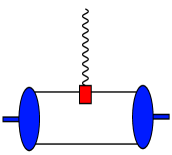
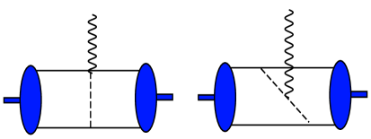
Fig. 16. : The impulse-approximation contribution to $G_{\mathrm{C}}$ and $G_{\mathrm{Q}}$ is shown on the left, while two meson-exchange current mechanisms which would contribute were the deuteron not an isoscalar target are depicted in the middle and on the right.

The most important correction that arises at NLO [$O(eP^{2})$] is the inclusion of nucleon structure in $\chi$PT. At this order isoscalar form factors are dominated by short-distance physics, and so the only correction to the point-like leading-order result comes from the inclusion of the nucleon’s electric radius, i.e.

$${G_{\mathrm{E}}^{\mathrm{(}s)}}_{\mbox{$\chi$PT NLO}}=1-\frac{1}{6}\langle r_{\mathrm{E}}^{{\mathrm{(}s)}\,2}\rangle q^{2}.$$ (131)

This description of nucleon structure breaks down at momentum transfers $q$ of order 300 MeV. There is a concomitant failure in the description of ed scattering data (see Figure 17). (This failure was already seen in the work of Meißner and Walzl [76].). In order to focus on deuteron structure, in the results presented below I have chosen to circumvent this issue by using a “factorized” inclusion of nucleon structure [77]. This facilitates the inclusion of experimentally-measured single-nucleon form factors in the calculation, thereby allowing us to test how far the theory is able to describe the two-body dynamics that takes place in ed scattering.

Fig. 17. : The deuteron charge form factor at orders $e$, $eP^{2}$ and $eP^{3}$ in a “strict” chiral perturbation theory calculation. The experimental data is taken from the compilation of Ref. [78].

We now compute results for $G_{\mathrm{C}}$ and $G_{\mathrm{Q}}$ at LO (structureless nucleons), NLO (adding nucleon structure and the first relativistic corrections), and N²LO (including the meson-exchange contribution discussed above in the charge operator $J_{0}$). This yields the parameter-free predictions shown in Fig. 18. The figure demonstrates that convergence is quite good below $q\sim 600$ MeV—especially for $G_{\mathrm{C}}$. The results shown are for the NLO chiral wave function, but the use of the NNLO chiral wave function, or indeed of simple wave functions which include only one-pion exchange, do not modify the picture greatly below $q=700$ MeV [77]. It is also clear that—provided the experimental data from electron-nucleon scattering is taken into account—$\chi$PT is capable of describing the charge and quadrupole form factors of deuterium at least as far as the minimum in $G_{\mathrm{C}}$. This result is encouraging for the application of EFT to light nuclei.

Fig. 18. : The deuteron charge and quadrupole form factors to order $eP^{3}$ in chiral perturbation theory, with the effects of nucleon structure included in the calculation. The experimental data is taken from the compilation of Ref. [78]. $G_{\mathrm{Q}}$ is in units of fm².

4.4 Compton scattering on deuterium

The scattering of low-energy photons from the nucleon at low energies probes the long-distance structure of the neutron and the proton. In the case of the neutron the low-energy Hamiltonian for the neutron’s interactions with photons is exactly (21). The coefficients of the ${\mathbf{E}}^{2}$ and ${\mathbf{B}}^{2}$ terms are related to the electric ($\alpha_{\mathrm{n}}$) and magnetic ($\beta_{\mathrm{n}}$) polarizability of the neutron via [4]:

$$a_{1}=-2\pi\alpha_{\mathrm{n}};\quad a_{2}=-2\pi\beta_{\mathrm{n}}.$$ (132)

Photon-nucleon scattering has been studied in $\chi$PT in Ref. [79, 80], where the following results for these neutron polarizabilities were obtained at leading non-vanishing order ($O(e^{2}P)$):

$$\alpha_{\mathrm{n}}={{5e^{2}g_{\mathrm{A}}^{2}}\over{384\pi^{2}f_{\pi}^{2}m_{\pi}}}=12.2\times 10^{-4}\,{\mathrm{f}m}^{3};~{}~{}\beta_{\mathrm{n}}={{e^{2}g_{\mathrm{A}}^{2}}\over{768\pi^{2}f_{\pi}^{2}m_{\pi}}}=1.2\times 10^{-4}\,{\mathrm{f}m}^{3}\,.$$ (133)

Chiral perturbation theory also predicts $\alpha_{\mathrm{n}}=\alpha_{\mathrm{p}}$, $\beta_{\mathrm{n}}=\beta_{\mathrm{p}}$ at this order. The processes which contribute at $O(e^{2}P)$ are those in which the photon interacts with the nucleon’s pion cloud. Recent experimental values for the proton polarizabilities are [81]:

$$\alpha_{\mathrm{p}}+\beta_{\mathrm{p}}=13.23\pm 0.86^{+0.20}_{-0.49}\times 10^{-4}\,{\mathrm{f}m}^{3},$$

$$\alpha_{\mathrm{p}}-\beta_{\mathrm{p}}=10.11\pm 1.74^{+1.22}_{-0.86}\times 10^{-4}\,{\mathrm{f}m}^{3}\,,$$ (134)

where the first error is a combined statistical and systematic error, and the second set of errors comes from the dispersion relation analysis used to extract $\alpha_{\mathrm{p}}$ and $\beta_{\mathrm{p}}$ from the experimental data. These values are in good agreement with the $\chi$PT predictions.

Meanwhile, the neutron polarizabilities $\alpha_{\mathrm{n}}$ and $\beta_{\mathrm{n}}$ are difficult to measure, due to the absence of free neutron targets, thus this prediction is not well tested. Hence there has been a considerable effort to extract $\alpha_{\mathrm{n}}$ and $\beta_{\mathrm{n}}$ by performing Compton scattering on nuclear targets. Coherent Compton scattering on a deuteron target has been measured at $E_{\gamma}=$ 49 and 69 MeV by the Illinois group [82] and $E_{\gamma}=84.2-104.5$ MeV at Saskatoon [83].

However, the amplitude for Compton scattering on the deuteron involves mechanisms other than Compton scattering on the individual nucleons inside the deuterium nucleus. Hence, if we want to extract neutron polarizabilities we will need a theoretical calculation of Compton scattering on the deuteron in which we can make sure that the error in our extraction of $\alpha_{\mathrm{n}}$ and $\beta_{\mathrm{n}}$ from subtracting out these “two-body” mechanisms is under control. $\chi$PT is an ideal framework for this, since the two-body mechanisms that contribute to $\gamma{\mathrm{d}}\rightarrow\gamma{\mathrm{d}}$ are calculable order-by-order in the chiral expansion, and so we can perform a consistent extraction of $\alpha_{\mathrm{n}}$ and $\beta_{\mathrm{n}}$. The theoretical error is defined as the size of the mistake made by neglecting terms of the next order in the expansion.

The Compton amplitude we wish to evaluate is (in the $\gamma d$ center-of-mass frame):

$$T^{\gamma{\mathrm{d}}}_{M^{\prime}\lambda^{\prime}M\lambda}({\mathbf{k}}^{\prime},{\mathbf{k}}) = \int{{\mathrm{d}}^{3}p\over(2\pi)^{3}}\,\,\psi_{M^{\prime}}\left({\mathbf{p}}+{{\mathbf{k}}-{\mathbf{k}}^{\prime}\over 2}\right)\,\,T_{\gamma{\mathrm{N}}_{\lambda^{\prime}\lambda}}({\mathbf{k}}^{\prime},{\mathbf{k}})\,\,\psi_{M}({\mathbf{p}})$$ (135)

$$+ \int{{{\mathrm{d}}^{3}p\,\,{\mathrm{d}}^{3}p^{\prime}}\over(2\pi)^{6}}\,\,\psi_{M^{\prime}}({\mathbf{p}}^{\prime})\,\,T^{\mathrm{2}N}_{\gamma{\mathrm{N}N}_{\lambda^{\prime}\lambda}}({\mathbf{k}}^{\prime},{\mathbf{k}})\,\,\psi_{M}({\mathbf{p}})$$

where $M$ ($M^{\prime}$) is the initial (final) deuteron spin state, and $\lambda$ ($\lambda^{\prime}$) is the initial (final) photon polarization state, and ${\mathbf{k}}$ (${\mathbf{k}}^{\prime}$) the initial (final) photon three-momentum, which are constrained to $|{\mathbf{k}}|=|{\mathbf{k}}^{\prime}|=\omega$. The amplitude $T_{\gamma{\mathrm{N}}}$ represents the graphs of Fig. 19 and Fig. 20b where the photon interacts with only one nucleon. These are the “one-body” mechanisms we actually wish to investigate. Meanwhile, the amplitude $T^{\mathrm{2}N}_{\gamma{\mathrm{N}N}}$ represents the graphs of Fig. 20a where there is an exchanged pion between the two nucleons. These are the “two-body” mechanisms we wish to calculate in a controlled way and then subtract them off.

Fig. 19. : Graphs which contribute to Compton scattering on the deuteron at ${\mathcal{}O}(e^{2})$ (a) and ${\mathcal{}O}(e^{2}P)$ (b-d). The sliced and diced blobs are from ${\mathcal{}L}_{\pi{\mathrm{N}}}^{(3)}$ (c) and ${\mathcal{}L}_{\pi\gamma}^{(4)}$ (d). Crossed graphs are not shown.

The LO contribution to Compton scattering on the deuteron is shown in Fig. 19(a). This graph involves a vertex from ${\mathcal{}L}_{\pi{\mathrm{N}}}^{(2)}$ and so is $O(e^{2})$. This contribution is simply the Thomson term for scattering on the proton. There is thus no sensitivity to either two-body contributions or nucleon polarizabilities at this order. At $O(e^{2}P)$ there are several more graphs with a spectator nucleon (Figs. 19(b),(c),(d)), as well as graphs involving an exchanged pion with leading order vertices (Fig. 20(a)) and one-loop graphs with a spectator nucleon (Fig. 20(b)) [84]. Graphs such as Fig. 20(b) contain the physics of the proton and neutron polarizabilities at $O(e^{2}P)$ in $\chi$PT.

Fig. 20. : Graphs which contribute to Compton scattering on the deuteron at ${\mathcal{}O}(e^{2}P)$. Crossed graphs are not shown.

The results shown below were generated with the NLO chiral wave function of Ref. [71]. Fig. 21 shows the results at $E_{\gamma}=$ 49, 69, and 95 MeV. For comparison we have included the calculation at $O(e^{2})$ in the kernel, where the second contribution in Eq. (135) is zero, and the single-scattering contribution is given solely by Fig. 19(a). At $O(e^{2}P)$ all contributions to the kernel are fixed in terms of known pion and nucleon parameters, so to this order $\chi$PT makes predictions for deuteron Compton scattering.

We also show the $O(e^{2}P^{2})$ result from work just being completed [65]. This calculation uses the NLO wave function of Ref. [71] and the $O(e^{2}P^{2})$ single-nucleon Compton amplitudes derived in Ref. [85]. Also included are a number of $1/M$ corrections to the two-body piece of the $\gamma{\mathrm{N}N}\rightarrow\gamma{\mathrm{N}N}$ amplitude. It turns out that such mechanisms are the only corrections to the two-body piece of this amplitude at this amplitude. In other words, no two-body counterterms contribute to $\gamma{\mathrm{d}}\rightarrow\gamma{\mathrm{d}}$ at $O(e^{2}P^{2})$. On the other hand, at $O(e^{2}P^{2})$ single-nucleon counterterms which shift the polarizabilities enter the calculation. But that is an advantage! It is exactly these counterterms—or more specifically the neutron counterterms—that we wish to extract from the $\gamma{\mathrm{d}}$ data, since these counterterms serve to fix the value of $\alpha_{\mathrm{n}}$, $\beta_{\mathrm{n}}$, $\alpha_{\mathrm{p}}$ and $\beta_{\mathrm{p}}$. In this sense Compton scattering on deuterium at $O(e^{2}P^{2})$ is analogous to the reaction $\gamma{\mathrm{d}}\rightarrow\pi^{0}{\mathrm{d}}$ [64]: an $O(e^{2}P^{2})$ calculation allows us to test the single-nucleon physics which is used to predict the results of coherent scattering on deuterium, since there are no undetermined parameters in the two-body mechanisms that enter to this order in the chiral expansion. For the calculations displayed here we have set the nucleon polarizabilities to the values:

$$\alpha_{\mathrm{p}}=\alpha_{\mathrm{n}}=12.0\times 10^{-4}~{}{\mathrm{f}m}^{3},$$ (136)

$$\beta_{\mathrm{p}}=\beta_{\mathrm{n}}=2.0\times 10^{-4}~{}{\mathrm{f}m}^{3}.$$ (137)

In fact the results for this observable are quite sensitive to $\alpha_{\mathrm{n}}$ and $\beta_{\mathrm{n}}$, so ultimately one would like to use experimental values for the proton polarizabilities, such as those quoted in Eq. (134), as well as performing a $\chi^{2}$ fit to the photon-deuteron experimental data in order to constrain the neutron $\alpha$ and $\beta$. This should become a more realistic option as data on $\gamma{\mathrm{d}}\rightarrow\gamma{\mathrm{d}}$ from Lund becomes available [86].

Fig. 21. : Results of the $O(e^{2})$ (dotted line), $O(e^{2}P)$ (dashed line), and $O(e^{2}P^{2})$ (solid line) calculations for $E_{\gamma}=49~{}{\mathrm{M}eV}$, $69~{}{\mathrm{M}eV}$ and $95~{}{\mathrm{M}eV}$ respectively from left to right.

The data shown in Fig. 21 includes six points from the Illinois experiment at 49 and 69 MeV [82] and the Saskatoon data at 95 MeV [83]. Statistical and systematic errors have been added in quadrature. It is quite remarkable how well the $O(e^{2})$ calculation reproduces the 49 MeV data. However, since there are sizeable higher-order corrections this agreement might be regarded as somewhat fortuitous . Meanwhile, the agreement of the $O(e^{2}P)$ calculation with the 69 MeV data is very good, although only limited conclusions can be drawn. Finally, the results at 95 MeV disagree markedly with the Saskatoon data, especially at backward angles. While this could be indicative that the neutron polarizabilities are starkly incorrect tests suggest that modifying $\alpha_{\mathrm{n}}$ and $\beta_{\mathrm{n}}$ in order to reproduce the backward-angle $\gamma{\mathrm{d}}$ data from Saskatoon would lead to disagreement between our calculations and the 69 MeV data.

In fact, similar conclusions have been reached in potential-model calculations [87, 88, 89] where the results for the differential cross sections are comparable to those obtained here using $\chi$PT. They are also not dissimilar to those obtained in NN EFTs without explicit pions (see Ref. [39]).

Many other processes have been computed using Weinberg power-counting. The application to $\pi{\mathrm{d}}$ scattering is intriguing, and holds promise of allowing for an extraction of the isoscalar $\pi{\mathrm{N}}$ scattering length [63, 68]. The prediction of the threshold amplitude for $\gamma{\mathrm{d}}\rightarrow\pi^{0}{\mathrm{d}}$ was a significant triumph for $\chi$PT applied to deuterium [64]. Meanwhile, Park, Min, Kubodera, Rho, and collaborators have calculated many processes, paying particular attention to astrophysical reactions. See Ref. [2, 90] for summaries of this work, which represents an important application of $\chi$PT in particular, and effective theories of nuclear physics in general.

References

- [1] U. van Kolck, Prog. Part. Nucl. Phys. 43, 409 (1999), nucl-th/9902015.
- [2] S. R. Beane, P. F. Bedaque, W. Haxton, D. R. Phillips, and M. J. Savage, (2000), nucl-th/0008064.
- [3] D. B. Kaplan, nucl-th/9506035.
- [4] B. R. Holstein, (2000), hep-ph/0010129.
- [5] J. D. Jackson, Classical Electrodynamics, 2nd edition, Wiley, New York, 1975.
- [6] I. J. R. Atchison and A. J. G. Hey, Gauge Theories in Particle Physics, 2nd edition, IOP Publishing, Bristol, 1989.
- [7] L. H. Ryder, Quantum Field Theory, Cambridge University Press, Cambdridge, 1985.
- [8] Renormalization: from Lorentz to Landau (and beyond), edited by L. M. Brown, Springer-Verlag, New York, 1993.
- [9] G. P. Lepage, What is renormalization?, in From Actions to Answers, edited by T. deGrand and D. Toussiant, Singapore, 1990, World Scientific.
- [10] G. P. Lepage, nucl-th/9706029.
- [11] H. A. Bethe, Phys. Rev. 76, 38 (1949).
- [12] H. A. Bethe and C. Longmire, Phys. Rev. 77, 647 (1950).
- [13] D. R. Phillips and T. D. Cohen, Phys. Lett. B390, 7 (1997), nucl-th/9607048.
- [14] D. B. Kaplan, M. Savage, and M. B. Wise, Nucl. Phys. B534, 329 (1998), nucl-th/9802075.
- [15] J. J. de Swart, C. P. F. Terheggen, and V. G. J. Stoks, (1995), nucl-th/9509032.
- [16] V. G. J. Stoks, R. A. M. Klomp, M. C. M. Rentmeester, and J. J. de Swart, Phys. Rev. C 48, 792 (1993).
- [17] J.-W. Chen, G. Rupak, and M. Savage, Nucl. Phys. A653, 386 (1999), nucl-th/9902056.
- [18] M. Luke and A. V. Manohar, Phys. Rev. D 55, 4129 (1997), hep-ph/9610534.
- [19] D. B. Kaplan, M. Savage, and M. B. Wise, Nucl. Phys. B478, 629 (1996), nucl-th/9605002.
- [20] M. Lutz, hep-ph/9606301.
- [21] U. van Kolck, Nucleon nucleon interaction and isospin violation, in Mainz 1997, Chiral Dynamics: Theory and Experiment, edited by A. M. Bernstein, D. Drechsel, and T. Walcher, Berlin, 1998, Springer-Verlag.
- [22] D. B. Kaplan, M. Savage, and M. B. Wise, Phys. Lett. B424, 390 (1998), nucl-th/9801034.
- [23] U. van Kolck, Nucl. Phys. A645, 273 (1999), nucl-th/9808007.
- [24] M. C. Birse, J. A. McGovern, and K. G. Richardson, PiN Newslett. 15, 280 (1999), nucl-th/9911048.
- [25] D. R. Phillips, G. Rupak, and M. J. Savage, Phys. Lett. B473, 209 (2000), nucl-th/9908054.
- [26] J. Gegelia, Phys. Lett. B429, 227 (1998).
- [27] J. Gegelia, J. Phys. G 25, 1681, nucl-th/9805008.
- [28] T. Mehen and I. W. Stewart, Phys. Lett. B445, 378, nucl-th/9809071.
- [29] K. A. Scaldeferri, D. R. Phillips, C.-W. Kao, and T. D. Cohen, Phys. Rev. C 56, 679 (1997), nucl-th/9610049.
- [30] D. B. Kaplan, Nucl. Phys. B494, 471 (1997), nucl-th/9610052.
- [31] S. Weinberg, Phys. Rev. 130, 776 (1963).
- [32] P. F. Bedaque and H. W. Griesshammer, Nucl. Phys. A671, 357 (2000), nucl-th/9907077.
- [33] S. R. Beane and M. J. Savage, Nucl. Phys. A694, 511 (2001), nucl-th/0011067.
- [34] V. G. J. Stoks, R. A. M. Klomp, C. P. F. Terheggen, and J. J. de Swart, Phys. Rev. C 49, 2950 (1994).
- [35] R. Gilman and F. Gross, (2001), nucl-th/0111015.
- [36] G. Rupak, Nucl. Phys. A678, 405 (2000), nucl-th/9911018.
- [37] M. Butler, J.-W. Chen, and X. Kong, Phys. Rev. C63, 035501 (2001), nucl-th/0008032.
- [38] M. Butler and J.-W. Chen, Phys. Lett. B520, 87 (2001), nucl-th/0101017.
- [39] H. W. Griesshammer and G. Rupak, (2000), nucl-th/0012096.
- [40] G. Rupak and X.-W. Kong, (2001), nucl-th/0108059.
- [41] Gospel of St. Matthew, Chapter 13, verse 52, New International Version.
- [42] B. F. Gibson, Nucl. Phys. A543, 1c (1992).
- [43] P. Bedaque and U. van Kolck, Phys. Lett. B428, 221, nucl-th/9710073.
- [44] P. F. Bedaque, H. W. Hammer, and U. van Kolck, Phys. Rev. C58, 641 (1998), nucl-th/9802057.
- [45] P. F. Bedaque, H. W. Hammer, and U. van Kolck, Phys. Rev. Lett. 82, 463 (1999), nucl-th/9809025.
- [46] P. F. Bedaque, H. W. Hammer, and U. van Kolck, Nucl. Phys. A646, 444 (1999), nucl-th/9811046.
- [47] G. Skornyakov and K. A. Ter-Martirosian, Soviet Physics JETP 4, 648 (1957).
- [48] J. Gegelia, Nucl. Phys. A680, 303 (2000), nucl-th/9903030.
- [49] G. S. Danilov, Soviet Physics JETP 16, 110 (1963).
- [50] V. N. Efimov, Phys. Rev. 44, 2303 (1991).
- [51] J. L. Friar, D. Huber, H. Witala, and G. L. Payne, Acta Phys. Polon. B31, 749 (2000), nucl-th/9908058.
- [52] F. Gabbiani, P. F. Bedaque, and H. W. Griesshammer, Nucl. Phys. A675, 601 (2000), nucl-th/9911034.
- [53] A. M. Perelomov and V. S. Popov, Teor. Mat. Fiz. 4, 664 (1970).
- [54] S. R. Beane, P. F. Bedaque, M. J. Savage, and U. van Kolck, (2001), nucl-th/0104030.
- [55] H. W. Hammer and T. Mehen, Phys. Lett. B516, 353 (2001), nucl-th/0105072.
- [56] P. F. Bedaque, H. W. Hammer, and U. van Kolck, Nucl. Phys. A676, 357 (2000), nucl-th/9906032.
- [57] A. C. Phillips, Nucl. Phys. A107, 209 (1968).
- [58] I. R. Afnan and F. J. D. Serduke, Phys. Lett. B. 44, 143 (1973).
- [59] R. J. Furnstahl, H. W. Hammer, and N. Tirfessa, Nucl. Phys. A689, 846 (2001), nucl-th/0010078.
- [60] V. Bernard, N. Kaiser, and U.-G. Meissner, Int. Jour. of Mod. Phys. E 4, 193 (1995), hep-ph/9501384.
- [61] H. Leutwyler, (2000), hep-ph/0008124.
- [62] U.-G. Meissner, (2000), hep-ph/0007092.
- [63] S. R. Beane, V. Bernard, T. S. H. Lee, and U. G. Meissner, Phys. Rev. C57, 424 (1998), nucl-th/9708035.
- [64] S. R. Beane, V. Bernard, T.-S. H. Lee, U.-G. Meissner, and U. van Kolck, Nucl. Phys. A618, 381 (1997), hep-ph/9702226.
- [65] S. R. Beane, J. McGovern, M. Malheiro, D. R. Phillips, and U. van Kolck, in preparation.
- [66] S. Weinberg, Phys. Lett. B251, 288 (1990).
- [67] S. Weinberg, Nucl. Phys. B363, 3 (1991).
- [68] S. Weinberg, Phys. Lett. B295, 114 (1992).
- [69] C. Ordonéz, L. Ray, and U. van Kolck, Phys. Rev. C 53, 2086 (1996), nucl-th/9511380.
- [70] N. Kaiser, R. Brockmann, and W. Weise, Nucl. Phys. A625, 758 (1997), nucl-th/9706045.
- [71] E. Epelbaum, W. Glockle, and U.-G. Meissner, Nucl. Phys. A671, 295 (1999), nucl-th/9910064.
- [72] M. C. M. Rentmeester, R. G. E. Timmermans, J. L. Friar, and J. J. de Swart, Phys. Rev. Lett. 82, 4992 (1999), nucl-th/9901054.
- [73] D. R. Entem and R. Machleidt, Phys. Lett. B524, 93 (2002), nucl-th/0108057.
- [74] D. R. Phillips and T. D. Cohen, Nucl. Phys. A668, 45 (2000), nucl-th/9906091.
- [75] D. O. Riska, Prog. Part. Nucl. Phys. 11, 199 (1984).
- [76] U.-G. Meissner and M. Walzl, (2001), nucl-th/0103020.
- [77] D. R. Phillips, in preparation.
- [78] JLAB t20, D. Abbott et al., Eur. Phys. J. A7, 421 (2000), nucl-ex/0002003.
- [79] V. Bernard, N. Kaiser, and U. G. Meissner, Nucl. Phys. B383, 442 (1992).
- [80] V. Bernard, N. Kaiser, J. Kambor, and U. G. Meissner, Nucl. Phys. B388, 315 (1992).
- [81] J. Tonnison, A. M. Sandorfi, S. Hoblit, and A. M. Nathan, Phys. Rev. Lett. 80, 4382 (1998), nucl-th/9801008.
- [82] M. A. Lucas, Compton scattering from the deuteron at intermediate energies, PhD thesis, University of Illinois, 1994, unpublished.
- [83] D. L. Hornidge et al., Phys. Rev. Lett. 84, 2334 (2000), nucl-ex/9909015.
- [84] S. R. Beane, M. Malheiro, D. R. Phillips, and U. van Kolck, Nucl. Phys. A656, 367 (1999), nucl-th/9905023.
- [85] J. A. McGovern, Phys. Rev. C63, 064608 (2001).
- [86] M. Lundin, talk at low-Q workshop, Halifax, Nova Scotia, August 2001.
- [87] T. Wilbois, P. Wilhelm, and H. Arenhovel, Few Bod. Sys. 9, 263 (1995).
- [88] M. I. Levchuk and A. I. L’vov, (1998), nucl-th/9809034.
- [89] J. J. Karakowski and G. A. Miller, Phys. Rev. C60, 014001 (1999), nucl-th/9901018.
- [90] T.-S. Park, K. Kubodera, D.-P. Min, and M. Rho, Nucl. Phys. A684, 101 (2001), nucl-th/0005069.