Bethe-Salpeter equation and a nonperturbative quark-gluon vertex

Abstract

A Ward-Takahashi identity preserving Bethe-Salpeter kernel can always be calculated explicitly from a dressed-quark-gluon vertex whose diagrammatic content is enumerable. We illustrate that fact using a vertex obtained via the complete resummation of dressed-gluon ladders. While this vertex is planar, the vertex-consistent kernel is nonplanar and that is true for any dressed vertex. In an exemplifying model the rainbow-ladder truncation of the gap and Bethe-Salpeter equations yields many results; e.g., $\pi$- and $\rho$-meson masses, that are changed little by including higher-order corrections. Repulsion generated by nonplanar diagrams in the vertex-consistent Bethe-Salpeter kernel for quark-quark scattering is sufficient to guarantee that diquark bound states do not exist.

I Introduction

Dynamical chiral symmetry breaking (DCSB) and confinement are keystones in an understanding of strong interaction observables and their explanation via a nonperturbative treatment of QCD. The gap equation fn:Eucl

$$S(p)^{-1}=Z_{2}\,(i\gamma\cdot p+m_{\rm bm})$$ (1)

$$+\,Z_{1}\int^{\Lambda}_{q}\,g^{2}D_{\mu\nu}(p-q)\frac{\lambda^{a}}{2}\gamma_{\mu}S(q)\Gamma^{a}_{\nu}(q,p)\,,$$

is an insightful tool that has long been used to explore the connection between these phenomena and the long-range behaviour of the interaction in QCD cdragw . In this equation: $D_{\mu\nu}(k)$ is the renormalised dressed-gluon propagator; $\Gamma^{a}_{\nu}(q;p)$ is the renormalised dressed-quark-gluon vertex; $m_{\rm bm}$ is the $\Lambda$-dependent current-quark bare mass that appears in the Lagrangian; and $\int^{\Lambda}_{q}:=\int^{\Lambda}d^{4}q/(2\pi)^{4}$ represents a translationally-invariant regularisation of the integral, with $\Lambda$ the regularisation mass-scale. The quark-gluon-vertex and quark wave function renormalisation constants, $Z_{1}(\zeta^{2},\Lambda^{2})$ and $Z_{2}(\zeta^{2},\Lambda^{2})$ respectively, depend on the renormalisation point and the regularisation mass-scale.

The solution of Eq. (1) is the dressed-quark propagator, which takes the form

$$S(p)^{-1} = i\gamma\cdot p\,A(p^{2},\zeta^{2})+B(p^{2},\zeta^{2})$$ (2)

$$= \frac{1}{Z(p^{2},\zeta^{2})}\left[i\gamma\cdot p+M(p^{2},\zeta^{2})\right]\,,$$

and is obtained by solving the gap equation subject to the renormalisation condition that at some large, spacelike $\zeta^{2}$

$$\left.S(p)^{-1}\right|_{p^{2}=\zeta^{2}}=i\gamma\cdot p+m(\zeta)\,,$$ (3)

where $m(\zeta)$ is the renormalised current-quark mass at the scale $\zeta$: $Z_{4}\,m(\zeta)=Z_{2}\,m_{\rm bm}$, with $Z_{4}$ the renormalisation constant for the scalar part of the quark self energy. At one loop in perturbation theory

$$m(\zeta)=\frac{\hat{m}}{\left(\ln[\zeta/\Lambda_{\rm QCD}]\right)^{\gamma_{m}}}\,,$$ (4)

where: $\hat{m}$ is the renormalisation-group-invariant current-quark mass; $\gamma_{m}=12/(33-2N_{f})$ is the leading-order mass anomalous dimension, for $N_{f}$ active flavours; and $\Lambda_{\rm QCD}$ is the $N_{f}$-flavour QCD mass-scale.

Since QCD is an asymptotically free theory the chiral limit is unambiguously defined by $\hat{m}=0$ mrt98 , which can be implemented in Eq. (1) by applying mr97

$$\lim_{\Lambda\to\infty}Z_{2}(\zeta^{2},\Lambda^{2})\,m(\Lambda)=0\,.$$ (5)

The formation of a gap, described by Eq. (1), is identified with the appearance of a solution for the dressed-quark propagator in which $m(\zeta)\sim{\rm O}(1/\zeta^{2})\neq 0$; i.e., a solution in which the mass function is power-law suppressed. This is DCSB. It is impossible at any finite order in perturbation theory and entails the appearance of a nonzero value for the vacuum quark condensate:

$$\,-\,\langle\bar{q}q\rangle_{\zeta}^{0}=\lim_{\Lambda\to\infty}Z_{4}(\zeta^{2},\Lambda^{2})\,N_{c}\,{\rm tr}_{\rm D}\int^{\Lambda}_{q}\!S^{0}(q,\zeta)\,,$$ (6)

where ${\rm tr}_{D}$ identifies a trace over Dirac indices alone and the superscript “$0$” indicates the quantity was calculated in the chiral limit.

It is apparent that the kernel of the gap equation is formed from a product of the dressed-gluon propagator and dressed-quark-gluon vertex. The kernel may be calculated in perturbation theory but that is inadequate for the study of intrinsically nonperturbative phenomena. Consequently, to make model-independent statements about DCSB one must employ an alternative systematic and chiral symmetry preserving truncation scheme.

One such scheme was introduced in Ref. truncscheme . Its leading-order term is the rainbow-ladder truncation of the DSEs and the general procedure provides a means to identify, a priori, those channels in which that truncation is likely to be accurate. This scheme underlies the successful application of a renormalisation-group-improved rainbow-ladder model to flavour-nonsinglet pseudoscalar mesons mr97 and vector mesons pieterrho ; pieterpion ; pieterpiK ; pieterother , and indicates why the leading-order truncation is inadequate for scalar mesons and flavour-singlet pseudoscalars cdrqcII . The systematic nature of the scheme has also made possible a proof of Goldstone’s theorem in QCD mrt98 .

In quantitative applications, however, the leading-order term alone has been used almost exclusively: Refs. pieterpiK ; arne are exceptions but they consider just the next-to-leading-order term. Hence one goal of our study is a nonperturbative verification of the leading-order truncation’s accuracy.

One element of the gap equation’s kernel is the dressed-gluon propagator, which in Landau gauge can be written

$$D_{\mu\nu}(k)=\left[\delta_{\mu\nu}-\frac{k_{\mu}k_{\nu}}{k^{2}}\right]\frac{d(k^{2},\zeta^{2})}{k^{2}}\,.$$ (7)

It has been the focus of DSE studies ragluon and lattice simulations tonylattice ; kurtlattice , and contemporary analyses suggest that $d(k^{2},\zeta^{2})/k^{2}$ is finite, and of O$(1\,{\rm GeV}^{-2})$, at $k^{2}=0$. However, this behaviour is difficult to reconcile with the existence and magnitude of DCSB in the strong interaction spectrum fredIR : it is a model-independent result that a description of observable phenomena requires a kernel in the gap equation with significant integrated strength on the domain $k^{2}\lesssim 1\,$GeV² cdresi . The required magnification may arise via an enhancement in the dressed-quark-gluon vertex but, hitherto, no calculation of the vertex exhibits such behaviour latticevertex . Hence another aim of our study is to contribute to the store of nonperturbative information about this vertex.

In Sec. II we briefly recapitulate on the truncation scheme of Ref. truncscheme . Then, using a simple confining model mn83 , we demonstrate that an infinite subclass of contributions to the dressed-quark-gluon vertex: the dressed-gluon ladders, can be resummed via an algebraic recursion relation, which provides a closed form result for the vertex expressed solely in terms of the dressed-quark propagator. This facilitates a simultaneous solution of the coupled gap and vertex equations obtained via the infinite resummation, as we describe in Sec. III. While the algebraic simplicity of these results is peculiar to our rudimentary model, we anticipate that the qualitative behaviour of the solutions is not.

In Sec. IV we describe the general procedure that enables a calculation of the Bethe-Salpeter kernel for flavour-nonsinglet mesons that is consistent with the fully-resummed dressed-gluon-ladder vertex. The kernel is itself a resummation of infinitely many diagrams; and it is not planar, an outcome necessary to ensure the preservation of Ward-Takahashi identities. This kernel is the heart of the inhomogeneous vertex equations and associated bound state equations whose solutions relate to strong interaction observables. In our simple model it, like the vertex, can also be obtained via an algebraic recursion relation, complete and in a practical closed form. In Sec. IV we also study the bound state equations in a number of meson channels, and derive and solve the analogous equation for diquark channels.

Section V is a summary.

II A Dressed-Quark-Gluon Vertex

The truncation scheme introduced in Ref. truncscheme may be described as a dressed-loop expansion of the dressed-quark-gluon vertices that appear in the half amputated dressed-quark-antiquark (or -quark-quark) scattering matrix: $S^{2}K$, a renormalisation-group invariant, where $K$ is the dressed-quark-antiquark (or -quark-quark) scattering kernel. All $n$-point functions involved thereafter in connecting two particular quark-gluon vertices are fully dressed. The effect of this truncation in the gap equation, Eq. (1), is realised through the following representation of the dressed-quark-gluon vertex, $i\Gamma_{\mu}^{a}=\mbox{\footnotesize$\displaystyle\frac{i}{2}$}\lambda^{a}\,\Gamma_{\mu}=l^{a}\Gamma_{\mu}$:

$$Z_{1}\Gamma_{\mu}(k,p)=\gamma_{\mu}$$ (8)

$$+ \mbox{\footnotesize$\displaystyle\frac{1}{2N_{c}}$}\int_{\ell}^{\Lambda}\!g^{2}D_{\rho\sigma}(p-\ell)\gamma_{\rho}S(\ell+k-p)\gamma_{\mu}S(\ell)\gamma_{\sigma}$$

$$+ \mbox{\footnotesize$\displaystyle\frac{N_{c}}{2}$}\int_{\ell}^{\Lambda}\!g^{2}\,D_{\sigma^{\prime}\sigma}(\ell)\,D_{\tau^{\prime}\tau}(\ell+k-p)\,$$

$$\times\,\gamma_{\tau^{\prime}}\,S(p-\ell)\,\gamma_{\sigma^{\prime}}\,\Gamma^{3g}_{\sigma\tau\mu}(\ell,-k,k-p)+[\ldots]\,.$$

Here $\Gamma^{3g}$ is the dressed-three-gluon vertex and it is apparent that the lowest order contribution to each term written explicitly is O$(g^{2})$. The ellipsis represents terms whose leading contribution is O$(g^{4})$; i.e., the crossed-box and two-rung dressed-gluon ladder diagrams, and also terms of higher leading-order.

The expansion of $S^{2}K$ just described, with its implications for other $n$-point functions; e.g., the dressed-quark-photon vertex, yields an ordered truncation of the DSEs that, term-by-term, guarantees the preservation of vector and axial-vector Ward-Takahashi identities, a feature exploited in Ref. mrt98 to prove Goldstone’s theorem. Furthermore, it is readily seen that inserting Eq. (8) into Eq. (1) provides the rule by which the renormalisation-group-improved rainbow-ladder truncation mr97 ; pieterrho ; pieterpion ; pieterpiK ; pieterother can be systematically improved. It thereby facilitates an explicit enumeration of corrections to the impulse current that is widely used in calculations of electroweak hadron form factors pieterpiK .

II.1 Resumming Dressed-Gluon Ladders

We can’t say anything about a complete resummation of the terms in Eq. (8). However, we are able to contribute to aspects of the more modest problem obtained by retaining only the sum of dressed-gluon ladders; i.e., aspects of the vertex depicted in Fig. 1. This infinite subclass of diagrams is $1/N_{c}$-suppressed.

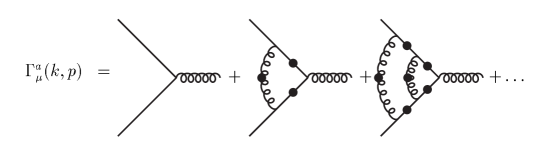
Figure 1: Integral equation for a planar dressed-quark-gluon vertex obtained by neglecting contributions associated with explicit gluon self-interactions. Solid circles indicate fully dressed propagators. The vertices are not dressed.

II.1.1 A Model

To simplify our analysis and make the key elements transparent we employ the confining model introduced in Ref. mn83 , which is defined by the following choice for the dressed-gluon line in Fig. 1:

$${\cal D}_{\mu\nu}(k):=g^{2}\,D_{\mu\nu}(k)=\left(\delta_{\mu\nu}-\frac{k_{\mu}k_{\nu}}{k^{2}}\right)(2\pi)^{4}\,{\cal G}^{2}\,\delta^{4}(k)\,.$$ (9)

Plainly, ${\cal G}$, measured in GeV, sets the model’s mass-scale and henceforth we set ${\cal G}=1$ so that all mass-dimensioned quantities are measured in units of ${\cal G}$. In the following, since the model is ultraviolet-finite, we usually remove the regularisation mass-scale to infinity and set the renormalisation constants equal to one.

The model defined by Eq. (9) is a precursor to an efficacious class of models that employ a renormalisation-group-improved effective interaction and whose contemporary application is reviewed in Refs. revbasti ; revreinhard . It has many positive features in common with that class and, furthermore, its particular momentum-dependence works to advantage in reducing integral equations to algebraic equations that preserve the character of the original equation. Naturally, there is a drawback: the simple momentum dependence also leads to some model-dependent artefacts, but they are easily identified and hence are not cause for concern.

II.1.2 Planar Vertex

The general form of the dressed-quark gluon vertex involves twelve distinct scalar form factors but using Eq. (9) that part of this vertex which contributes to the gap equation has no dependence on the total momentum of the quark-antiquark pair; i.e., only $\Gamma_{\mu}(p):=\Gamma_{\mu}(p,p)$ contributes. This considerably simplifies the analysis since, in general, one can write

$$\Gamma_{\mu}(p) = \alpha_{1}(p^{2})\,\gamma_{\mu}+\,\alpha_{2}(p^{2})\,\gamma\cdot p\,p_{\mu}$$ (10)

$$-\,\alpha_{3}(p^{2})\,i\,p_{\mu}+\alpha_{4}(p^{2})\,i\gamma_{\mu}\,\gamma\cdot p\,,$$

but it does not restrict our ability to address the questions we raised in the introduction because those amplitudes which survive are the most significant in the dressed-quark-photon vertex pieterpion and it is an enhancement in the vicinity of $p^{2}=0$ that may be important for a realisation of DCSB using an infrared-finite dressed-gluon propagator fredIR .

The summation depicted in Fig. 1 is expressed via

$$\Gamma_{\mu}(p_{+},p_{-})=Z_{1}^{-1}\gamma_{\mu}$$

$$+\,\mbox{\footnotesize$\displaystyle\frac{1}{6}$}\int_{\ell}^{\Lambda}\!\,{\cal D}_{\rho\sigma}(p-\ell)\gamma_{\rho}\,S(\ell_{+})\,\Gamma_{\mu}(\ell_{+},\ell_{-})\,S(\ell_{-})\,\gamma_{\sigma}$$

with $v_{\pm}=v\pm\mbox{\footnotesize$\displaystyle\frac{1}{2}$}P$, where $v=\ell,p$, etc., is any four-vector, but using Eq. (9) this simplifies to

$$\Gamma_{\mu}(p)=\gamma_{\mu}+\mbox{\footnotesize$\displaystyle\frac{1}{8}$}\,\gamma_{\rho}\,S(p)\,\Gamma_{\mu}(p)\,S(p)\,\gamma_{\rho}\,,$$ (12)

where the additional factor of $3/4$ ($1/8$ cf. $1/6$) owes itself to the combined operation of the $\delta$-function and the longitudinal projection operator. Inserting Eq. (10) into Eq. (12) one finds $\alpha_{4}\equiv 0$ and hence the solution of Eq. (12) simplifies:

$$\Gamma_{\mu}(p)=\alpha_{1}(p^{2})\,\gamma_{\mu}+\,\alpha_{2}(p^{2})\,\gamma\cdot p\,p_{\mu}-\,\alpha_{3}(p^{2})\,i\,p_{\mu}\,.$$ (13)

We re-express this vertex as

$$\Gamma_{\mu}(p)=\sum_{i=0}^{\infty}\,\Gamma_{\mu}^{i}(p)$$

$$= \sum_{i=0}^{\infty}\,\left[\alpha^{i}_{1}(p^{2})\,\gamma_{\mu}+\,\alpha^{i}_{2}(p^{2})\,\gamma\cdot p\,p_{\mu}-\,\alpha^{i}_{3}(p^{2})\,i\,p_{\mu}\right],$$

where the superscript enumerates the order of the iterate: $\Gamma_{\mu}^{i=0}$ is the bare vertex,

$$\begin{array}[]{cc}\alpha_{1}^{0}=1\,,&\alpha_{2}^{0}=0=\alpha_{3}^{0}\,;\end{array}$$ (16)

$\Gamma_{\mu}^{i=1}$ is the result of inserting this into the r.h.s. of Eq (12) to obtain the one-rung dressed-gluon correction; $\Gamma_{\mu}^{i=2}$ is the result of inserting $\Gamma_{\mu}^{i=1}$, and is therefore the two-rung dressed-gluon correction; etc.

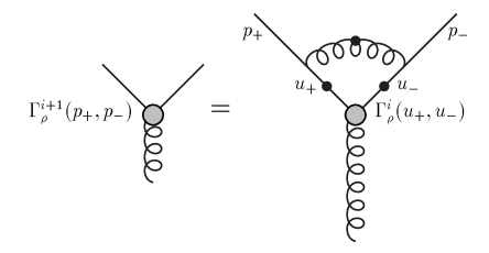
Figure 2: Recursion relation for the iterates in the fully-resummed dressed-gluon-ladder vertex, Eq. (LABEL:vtxrecursfull): filled circles denote a fully-dressed propagator or vertex. Using Eq. (9), $p=k$, and this relation is expressed by Eq. (18).

Now a simple but important observation is that each iterate is related to its precursor via the following recursion relation:

$$\Gamma_{\rho}^{a;i+1}(p_{+},p_{-}):=l^{a}\,\Gamma_{\rho}^{i+1}(p_{+},p_{-})=$$

$$\int_{u}^{\Lambda}\!{\cal D}_{\mu\nu}(p-u)\,l^{b}\gamma_{\mu}\,S(u_{+})\,l^{a}\Gamma_{\rho}^{i}(u_{+},u_{-})\,S(u_{-})\,l^{b}\gamma_{\nu}\,,$$

which is depicted in Fig. 2. Using Eq. (9) this simplifies:

$$\Gamma_{\rho}^{i+1}(p)=\mbox{\footnotesize$\displaystyle\frac{1}{8}$}\,\gamma_{\mu}\,S(p)\,\Gamma_{\rho}^{i}(p)\,S(p)\,\gamma_{\mu}$$ (18)

and substituting Eq. (LABEL:vtxi) into Eq. (18) yields ($s=p^{2}$)

$$\mbox{\boldmath$\alpha$}^{i+1}(s):=\left(\begin{array}[]{l}\rule{0.0pt}{10.76385pt}\alpha_{1}^{i+1}(s)\\ \rule{0.0pt}{10.76385pt}\alpha_{2}^{i+1}(s)\\ \rule{0.0pt}{10.76385pt}\alpha_{3}^{i+1}(s)\end{array}\right)={\cal O}(s;A,B)\,\mbox{\boldmath$\alpha$}^{i}(s)\,,$$ (19)

$${\cal O}(s;A,B)=\mbox{\footnotesize$\displaystyle\frac{1}{4}$}\,\frac{1}{(sA^{2}+B^{2})^{2}}$$ (23)

$$\times\left(\begin{array}[]{ccc}\rule{0.0pt}{10.76385pt}-(sA^{2}+B^{2})&0&0\\ \rule{0.0pt}{10.76385pt}2A^{2}&sA^{2}-B^{2}&2AB\\ \rule{0.0pt}{10.76385pt}4AB&4sAB&2(B^{2}-sA^{2})\end{array}\right).$$

Now it is clear that Eqs. (13), (LABEL:vtxi), (19) entail

$$\mbox{\boldmath$\alpha$}=\left(\sum_{i=1}^{\infty}\,{\cal O}^{i}\right)\,\mbox{\boldmath$\alpha$}^{0}=\frac{1}{1-{\cal O}}\,\mbox{\boldmath$\alpha$}^{0}\,,$$ (25)

where the last step is valid whenever an iterative solution of Eq. (LABEL:GammainfEq) exists, and defines a solution otherwise, so that, with $\Delta=sA^{2}(s)+B^{2}(s)$,

$$\alpha_{1} = \frac{4\,\Delta}{1+4\,\Delta}\,,$$

$$\alpha_{2} = \frac{-\,8\,A^{2}}{1+2\,(B^{2}-s\,A^{2})-8\,\Delta^{2}}\,\frac{1+2\,\Delta}{1+4\,\Delta}\,,$$ (26)

$$\alpha_{3} = \frac{-8\,AB}{1+2(B^{2}-s\,A^{2})-8\,\Delta^{2}}\,.$$

We have thus arrived at a closed form for the gluon-ladder-dressed quark-gluon vertex of Fig. 1; i.e., Eqs. (13), (26). Its momentum-dependence is determined by that of the dressed-quark propagator, which is obtained by solving the gap equation, itself constructed with this vertex. Using Eq. (9) that gap equation is

$$S(p)^{-1}=\left\{\begin{array}[]{l}i\gamma\cdot p+m+\gamma_{\mu}\,S(p)\,\Gamma_{\mu}(p)\\ \rule{0.0pt}{12.91663pt}i\gamma\cdot p+m+\Gamma_{\mu}(p)\,S(p)\,\gamma_{\mu}\end{array}\right.$$ (27)

and substituting Eq. (13) this gives

$$A(s) = 1+\frac{1}{sA^{2}+B^{2}}\left[A\,(2\alpha_{1}-s\alpha_{2})-B\,\alpha_{3}\right]\,,$$

$$B(s) = m+\frac{1}{sA^{2}+B^{2}}\left[B\,(4\alpha_{1}+s\alpha_{2})-sA\,\alpha_{3}\right]\,.$$

(29)

Obviously, Eqs. (LABEL:Afull), (29), completed using Eqs. (26), form a closed, algebraic system. It can easily be solved numerically, and that procedure yields simultaneously the complete gluon-ladder-dressed vertex and the propagator for a quark fully dressed via gluons coupling through this nonperturbative vertex.

We note here that in the chiral limit a realisation of chiral symmetry in the Wigner-Weyl mode is always possible. This realisation is expressed via the $B\equiv 0$ solution of the gap equation, which from Eqs. (26), (29) is evidently always admissible for $m=0$.

III Solutions of the Gap and Vertex Equations

III.1 Algebraic Results

Before reporting results obtained via a numerical solution we consider a special case that signals the magnitude of the effects produced by the complete resummation in Fig. 1; i.e., we focus on the solutions at $s=0$. In this instance Eqs. (26) give, with $A_{0}=A(0)$, $B_{0}=B(0)$,

$$\alpha_{1}(s=0) = \displaystyle\frac{4\,B_{0}^{2}}{1+4\,B_{0}^{2}}\,,$$

$$\alpha_{2}(s=0) = \displaystyle\frac{8\,A_{0}^{2}}{(4\,B_{0}^{2}+1)^{2}}\,\frac{2\,B_{0}^{2}+1}{2\,B_{0}^{2}-1}\,,$$ (30)

$$\alpha_{3}(s=0) = \displaystyle\frac{8\,A_{0}\,B_{0}}{4\,B_{0}^{2}+1}\,\frac{1}{2\,B_{0}^{2}-1}\,.$$

Substituting these expressions, Eq. (29) becomes

$$B_{0}=m+\frac{16\,B_{0}}{4\,B_{0}^{2}+1}\,$$ (31)

and in the chiral limit this yields

$$B_{0}=\mbox{\footnotesize$\displaystyle\frac{1}{2}$}\,\sqrt{15}\approx 1.94\,,$$ (32)

which makes plain that the model specified by Eq. (9) supports a realisation of chiral symmetry in the Nambu-Goldstone mode; i.e., DCSB. The value in Eq. (32) can be compared with that obtained using the bare vertex; i.e., the leading-order term in the truncation of Ref. truncscheme : $B_{0}^{(0)}=2$, to see that the completely resummed dressed-gluon-ladder vertex alters $B_{0}$ by only $-3\,$%.

Similarly, Eq. (LABEL:Afull) becomes

$$A_{0}=1+\frac{8\,A_{0}}{4\,B_{0}^{2}+1}\left[1+\frac{1}{2\,B_{0}^{2}-1}\right]\,,$$ (33)

which using Eq. (32) gives

$$A_{0}=\frac{26}{15}\approx 1.73\,.$$ (34)

This, too, may be compared with the leading-order result: $A_{0}^{(0)}=2$. Again the resummation does not materially affect the value: here the change is $-13\,$%.

Inserting Eqs. (32), (34) into Eqs. (30) one finds

$$\begin{array}[]{lcccll}\alpha_{1}(0)&=&\mbox{\footnotesize$\displaystyle\frac{15}{16}$}&\approx&0.94&{\rm cf.}~{}1.0\,,\\[8.61108pt] \alpha_{2}(0)&=&\mbox{\footnotesize$\displaystyle\frac{221}{1800}$}&\approx&0.12&{\rm cf.}~{}0.0\,,\\[8.61108pt] \alpha_{3}(0)&=&\mbox{\footnotesize$\displaystyle\frac{1}{\sqrt{15}}$}&\approx&0.26&{\rm cf.}~{}0.0\,,\end{array}$$ (35)

where the last, comparative column lists the values for the leading-order (bare) vertex. It is evident that the solution of Eq. (LABEL:GammainfEq) obtained using an infrared amplified effective interaction, Eq. (9), which supports DCSB (and also confinement fn:confinement ), does not exhibit an enhancement in a neighbourhood of $p^{2}=0$. This provides an internally consistent picture: a dressed-quark-antiquark scattering kernel, whose embedding in the gap equation already possesses sufficient integrable strength, does not additionally magnify itself.

III.2 Numerical Results

III.2.1 Wigner-Weyl Mode

The $B\equiv 0$ solution of Eq. (29) is always admitted when $m=0$. In that case Eq. (LABEL:Afull) becomes

$$A(s)=1+\frac{8\,A(s)}{1+4\,s\,A^{2}(s)}\left[1+\frac{1}{1-4\,s\,A^{2}(s)}\right]\,,$$ (36)

of which there is no closed-form solution. (It is a quintic equation for $A(s)$.)

Figure 3: Numerical solution of Eq. (36): solid line; cf. the solution obtained with the bare vertex: dotted line; and the one-loop corrected vertex: dashed line.

However, using the bare vertex one finds a chiral limit solution: $A^{(0)}(s)=\sqrt{2/s}$ for $s\approx 0$. We therefore suppose that in the neighbourhood of $s=0$ Eq. (36) admits a solution of the form

$$A_{s\sim 0}(s)=\left(\frac{\kappa_{A}}{s}\right)^{1/2}\,.$$ (37)

Substituting this into Eq. (36) yields

$$1=\frac{16}{1+4\,\kappa_{A}}\,\frac{1-2\,\kappa_{A}}{1-4\,\kappa_{A}}\,,$$ (38)

which has two solutions: $\kappa_{A}=3/4$, $5/4$. The required (physical) solution of Eq. (36) satisfies $A(s)\stackrel{{\scriptstyle s\to\infty}}{{\to}}1^{+}$. Therefore $sA^{2}(s)\to sA^{2}_{s\sim 0}$ from above and hence the physical branch of the solution is described by

$$\kappa_{A}=\mbox{\footnotesize$\displaystyle\frac{5}{4}$}\,<2\,.$$ (39)

Evidently, in the chirally symmetric case too, the ladder-dressed vertex reduces the magnitude of the solution.

These features are apparent in the complete numerical solution of Eq. (36), which is depicted in Fig. 3. Furthermore, the gluon-ladder-dressed vertex, Eq. (13), obtained with this solution does not exhibit an enhancement.

III.2.2 Nambu-Goldstone Mode

Figure 4: Upper panel – $A(s)$, $M(s)$ obtained with $m=0$: solid line; Lower panel – $A(s)$, $M(s)$ obtained with $m=0.023$: solid line. All dimensioned quantities are expressed in units of ${\cal G}$ in Eq. (9). A fit to meson observables requires ${\cal G}\approx 0.5\,{\rm GeV}$ and hence this value of the current-quark mass corresponds to $\approx 10\,$MeV. In both panels, for comparison, we also plot the results obtained with the zeroth-order vertex: dotted line; and the one-loop vertex: dashed line.

Figure 5: The dressed-quark propagator can be written: $S(p)=-i\gamma\cdot p\,\sigma_{V}(s)+\sigma_{S}(s)$. Here we plot $4\,\sigma_{V}(s)$, $2\,\sigma_{S}(s)$ obtained with $m=0.023$ cf. the results obtained with the zeroth-order vertex: dotted line; and the one-loop vertex: dashed line. Clearly, the analytic properties of the dressed-quark propagator are qualitatively unaffected by our dressing of the vertex.

Figure 6: $\alpha_{i}$, $i=1,2,3$, calculated with $m=0.023$. These functions calculated at one-loop (dotted line) and two-loop (dashed line) are also plotted for comparison. The results obtained with $m=0$ are little different.

Figure 7: $\alpha_{i}$, $i=1,2,3$, calculated from Eqs. (41) using the dressed-quark propagator solutions obtained in Ref. entireCJB .

In Sec. III.1 we described features of the Nambu-Goldstone mode solution of the gap equation, whose $p^{2}\simeq 0$ properties are smoothly related to those of the $m\neq 0$ solution, as is also the case in QCD mishaSVY . A complete solution is only available numerically and our calculated results for the dressed-quark propagator and gluon-ladder-dressed vertex are depicted in Figs. 4 – 6.

It is apparent from the figures that the complete resummation of dressed-gluon ladders yields a result for the dressed-quark propagator that is little different from that obtained with the one-loop-corrected vertex; and there is no material difference from the result obtained using the zeroth-order vertex. A single, exemplary quantification of this observation is provided by a comparison between the values of $M(s=0)=B(0)/A(0)$ calculated using vertices dressed at different orders:

$$\begin{array}[]{l|llll}\sum_{i=0,N}\Gamma_{\mu}^{i}&N=0&N=1&N=2&N=\infty\\[6.45831pt] \hline\cr M(0)&\rule{0.0pt}{8.61108pt}1&1.105&1.115&1.117\end{array}$$ (40)

Similar observations apply to the vertex itself. Of course, there is a qualitative difference between the zeroth-order vertex and the one-loop-corrected result: $\alpha_{2,3}\neq 0$ in the latter case. However, once that effect is seeded, the higher-loop corrections do little.

III.2.3 Vertex Ansatz

In the absence of a nonperturbatively dressed quark-gluon vertex a number of phenomenological DSE studies have employed an Ansatz, which is based on a nonperturbative analysis of QED and, in particular, is constrained by the vector Ward-Takahashi identity and the requirement of multiplicative renormalisability BCMike . That vertex has been used entireCJB with the model interaction of Eq. (9) in which its form is expressed via

$$\alpha_{1}(s)=A(s)\,,\;\alpha_{2}(s)=2\,\frac{dA(s)}{ds}\,,\;\alpha_{3}(s)=2\,\frac{dB(s)}{ds}\,.$$ (41)

The functions defined by these expressions, calculated using the self-consistent solutions determined in Ref. entireCJB , are depicted in Fig. 7. They bear little resemblance to the functions obtained systematically via the resummation of dressed-gluon ladders, an outcome that could be anticipated based on the difference between the dressed-quark propagator calculated herein and that in Ref. entireCJB . This finding does not invalidate the Ansatz nor its use in modelling QCD but merely shows that the Ansatz cannot be a sum of dressed-gluon ladders alone.

IV Bethe-Salpeter Equation

The renormalised homogeneous Bethe-Salpeter equation (BSE) for the quark-antiquark channel denoted by $M$ can compactly be expressed as

$$[\Gamma_{M}(k;P)]_{EF}=\int_{q}^{\Lambda}\![K(k,q;P)]_{EF}^{GH}\,[\chi_{M}(q;P)]_{GH}$$ (42)

where: $\Gamma_{M}(k;P)$ is the meson’s Bethe-Salpeter amplitude, $k$ is the relative momentum of the quark-antiquark pair and $P$ is their total momentum; $E,\ldots,H$ represent colour, flavour and spinor indices; and

$$\chi_{M}(k;P)=S(k_{+})\,\Gamma_{M}(k;P)\,S(k_{-})\,.$$ (43)

In Eq. (42), which is depicted in Fig. 8, $K$ is the fully-amputated dressed-quark-antiquark scattering kernel. The choice

$$[K(k,q;P)]_{EF}^{GH}={\cal D}_{\mu\nu}(k-q)\left[l^{a}\gamma_{\mu}\right]_{EG}\,\left[l^{a}\gamma_{\nu}\right]_{HF}\,,$$ (44)

yields the dressed-gluon ladder-truncation of the BSE, which provides the foundation for many contemporary, field-theory-based phenomenological studies of meson properties, see, e.g., Refs. lucha .

IV.1 Vertex-consistent Kernel

The preservation of Ward-Takahashi identities in those channels related to strong interaction observables requires a conspiracy between the dressed-quark-gluon vertex and the Bethe-Salpeter kernel truncscheme ; herman . We now describe a systematic procedure for building that kernel.

As described, e.g., in Ref. herman , the DSE for the dressed-quark propagator, $S$, is expressed via

$$\frac{\delta\Gamma[S]}{\delta S}=0\,,$$ (45)

where $\Gamma[S]$ is a Cornwall-Jackiw-Tomboulis-like effective action. The Bethe-Salpeter kernel is then obtained via an additional functional derivative:

$$K_{EF}^{GH}=-\frac{\delta\Sigma_{EF}}{\delta S_{GH}}\,.$$ (46)

Herein the self energy is given by the gap equation, Eq. (27), and the recursive nature of the dressed-gluon-ladder vertex entails that the $n$-th order contribution to the kernel is obtained from the $n$-loop contribution to the self energy:

$$\Sigma^{n}(p)=-\int_{q}^{\Lambda}\!{\cal D}_{\mu\nu}(p-q)\,l^{a}\gamma_{\mu}\,S(q)l^{a}\,\Gamma_{\nu}^{n}(q,p).$$ (47)

Since $\Gamma_{\mu}(p,q)$ itself depends on $S$ then Eq. (46) yields a sum of two terms:

$$[K^{n}(k,q;P)]_{EF}^{GH}$$ (48)

$$= {\cal D}_{\mu\nu}(k-q)\left[l^{a}\gamma_{\mu}\right]_{EG}\,\left[l^{a}\,\Gamma_{\nu}^{n}(q_{-},k_{-})\right]_{HF}$$

$$+\int_{\ell}^{\Lambda}\,{\cal D}_{\mu\nu}(k-\ell)\left[l^{a}\gamma_{\mu}\,S(\ell_{+})\right]_{EL}\,$$

$$\;\;\;\;\;\;\;\;\times\frac{\delta}{\delta S_{GH}(q_{\pm})}\left[l^{a}\,\Gamma_{\nu}^{n}(\ell_{-},k_{-})\right]_{LF}\,.$$

Here, in addition to the usual effect of differentiation, the functional derivative adds $P$ to the argument of every quark line through which it is commuted when applying the product rule. NB. ${\cal D}_{\mu\nu}$ also depends on $S$ because of quark vacuum polarisation diagrams. However, as noted in Ref. truncscheme , the additional term arising from the derivative of ${\cal D}_{\mu\nu}$ does not contribute to the BSE kernel for flavour non-diagonal systems, which are our focus herein, and hence is neglected for simplicity. It must be included though to obtain a kernel adequate for an analysis of problems such as the $\eta$-$\eta^{\prime}$ mass splitting, for example.

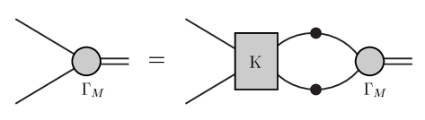
Figure 8: Homogeneous BSE, Eq. (42). Filled circles: dressed propagators or vertices; $K$ is the dressed-quark-antiquark scattering kernel. A systematic truncation of $S^{2}K$ is the key to preserving Ward-Takahashi identities truncscheme ; herman .

Now, introducing $[\chi_{M}(q;P)]_{GH}$, the BSE becomes

$$\Gamma_{M}(k;P)=\int_{q}^{\Lambda}{\cal D}_{\mu\nu}(k-q)\,$$

$$\times\,l^{a}\gamma_{\mu}\left[\rule{0.0pt}{12.91663pt}\chi_{M}(q;P)\,l^{a}\,\Gamma_{\nu}(q_{-},k_{-})+S(q_{+})\,\Lambda_{M\nu}^{a}(q,k;P)\right],$$

where we have used Eq. (II.1.2) and defined

$$\Lambda_{M\nu}^{a}(q,k;P)=\sum_{n=0}^{\infty}\Lambda_{M\nu}^{a;n}(q,k;P)\,,$$ (50)

with

$$\left[\Lambda^{a;n}_{M\nu}(\ell,k;P)\right]_{LF}=$$

$$\int_{q}^{\Lambda}\!\frac{\delta}{\delta S(q_{\pm})_{GH}}\left[l^{a}\,\Gamma_{\nu}^{n}(\ell_{-},k_{-})\right]_{LF}[\chi_{M}(q;P)]_{GH}\,.$$

Equation (LABEL:genbsenL1) is depicted in Fig. 9. The first term is instantly available once one has an explicit form for $\Gamma^{n}_{\nu}$. To develop an understanding of the second term, which is identified by the shaded box in the figure, we employ the recursive expression for the dressed-quark-gluon vertex, Eq. (LABEL:vtxrecursfull), with $p=k$, $P=\ell-k$, to obtain an inhomogeneous recursion relation for $\Lambda_{M\nu}^{a;n}$:

$$\Lambda^{a;n}_{M\nu}(\ell,k;P) = \int_{q}^{\Lambda}\!{\cal D}_{\rho\sigma}(\ell-q)\,l^{b}\gamma_{\rho}\,\chi_{M}(q;P)\,l^{a}\Gamma_{\nu}^{n-1}(q_{-},q_{-}+k-\ell)\,S(q_{-}+k-\ell)\,l^{b}\gamma_{\sigma}$$ (52)

$$+\int_{q}^{\Lambda}\!{\cal D}_{\rho\sigma}(k-q)\,l^{b}\gamma_{\rho}\,S(q_{+}+\ell-k)\,l^{a}\Gamma_{\nu}^{n-1}(q_{+}+\ell-k,q_{+})\,\chi_{M}(q;P)\,l^{b}\gamma_{\sigma}$$

$$+\int_{q^{\prime}}^{\Lambda}\!{\cal D}_{\rho\sigma}(\ell-q^{\prime})l^{b}\gamma_{\rho}\,S(q^{\prime}_{+})\,\Lambda^{a;n-1}_{M\nu}(q^{\prime},q^{\prime}+k-\ell;P)\,S(q_{-}^{\prime}+k-\ell)\,l^{b}\gamma_{\sigma}\,.$$

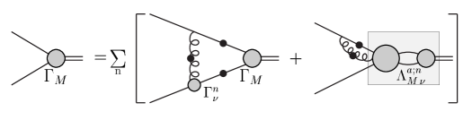
Figure 9: BSE expressed in Eq. (LABEL:genbsenL1), which is valid whenever $\Gamma_{\mu}$ can be obtained via a recursion relation.

Equation (52) is illustrated in Fig. 10 and, combined with Figs. 2, 9, this discloses the content of the vertex-consistent Bethe-Salpeter kernel: namely, it consists of a countable infinity of contributions, an infinite subclass of which are crossed-ladder diagrams and hence nonplanar. It is clear that every $n>0$, vertex-consistent kernel must contain nonplanar diagrams. Charge conjugation can be used to expose a diagrammatic symmetry in the Bethe-Salpeter kernel, which is the procedure we used, e.g., to obtain Eq. (27). (The steps and outcome described here formalise the procedure illustrated in Fig. 1 of Ref. truncscheme .)

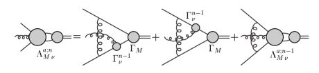
Figure 10: Recursion relation for $\Lambda_{M\nu}^{a;n}$, Eq. (52). We label the diagrams on the r.h.s., from left to right, as ${\cal G}_{1}$, ${\cal G}_{2}$, ${\cal L}$.

At this point if $\Gamma^{n}_{\nu}$ and the propagator functions: $A$, $B$, are known, then $\Lambda_{M\nu}^{a}$, and hence the channel-projected Bethe-Salpeter kernel, can be calculated explicitly. That needs to be done separately for each channel because, e.g., $\Lambda_{M\nu}^{a}$ depends on $\chi_{M}(q;P)$.

To proceed we observe that the Bethe-Salpeter amplitude for a $\pi$-meson is

$$\Gamma_{\pi}^{j}(k;P)=\mbox{\boldmath$I$}_{c}\,\tau^{j}\,\gamma_{5}\,\left[if^{1}_{\pi}(k^{2},k\cdot P;P^{2})\right.$$ (53)

$$+\,\gamma\cdot P\,f^{2}_{\pi}(k^{2},k\cdot P;P^{2})+\gamma\cdot k\,k\cdot P\,f^{3}_{\pi}(k^{2},k\cdot P;P^{2})$$

$$\left.+\,\sigma_{\mu\nu}k_{\mu}P_{\nu}\,f^{4}_{\pi}(k^{2},k\cdot P;P^{2})\right]\,,$$

where $\mbox{\boldmath$I$}_{c}$ is the identity in colour space (mesons are colour singlets) and $\{\tau^{j};j=1,2,3\}$ are the Pauli matrices. This illustrates the general structure of meson Bethe-Salpeter amplitudes, which hereafter we express via

$$\Gamma_{M}(k;P)=\mbox{\boldmath$I$}_{c}\sum_{i=1}^{N_{M}}\,{\cal G}^{i}(k;P)\,f^{i}_{M}(k^{2},k\cdot P;P^{2})\,,$$ (54)

where ${\cal G}^{i}(k;P)$ are the independent Dirac matrices required to span the space containing the meson under consideration. (Subsequently, to simplify our analysis, we focus on $N_{f}=2$ and assume isospin symmetry. There is no impediment, in principle, to a generalisation.)

The result of substituting Eq. (54) into the r.h.s. of Eq. (LABEL:genbsenL1) can be expressed in the compact form

$$\mbox{\boldmath$f$}={\cal H}\mbox{\boldmath$f$}=({\cal H}_{1}+{\cal H}_{2})\mbox{\boldmath$f$}\,,$$ (55)

where $f$ is a column vector composed of the scalar functions: $\mbox{\boldmath$f$}_{i}=f^{i}_{M}$. Here ${\cal H}_{1}$ is the contribution from the first term on the r.h.s. in Eq. (LABEL:genbsenL1) and it is a $N_{M}\times N_{M}$ matrix wherein the elements of row-$j$ are obtained via that Dirac trace projection which yields $f^{j}_{M}$ on the l.h.s.; i.e., for ${\cal P}_{j}$ such that

$$f^{j}_{M}={\rm tr}_{D}\left[{\cal P}_{j}\Gamma_{M}\right],$$ (56)

then, using $l^{a}\,l^{a}=-C_{2}(R)=-\mbox{\footnotesize$\displaystyle\frac{4}{3}$}$ for $SU(N_{c}=3)$,

$$[{\cal H}_{1}]_{j,k}\mbox{\boldmath$f$}_{k}=-\mbox{\footnotesize$\displaystyle\frac{4}{3}$}\,{\rm tr}_{D}\left[{\cal P}_{j}\,\int_{\ell}^{\Lambda}{\cal D}_{\mu\nu}(k-\ell)\gamma_{\mu}\,S(\ell_{+})\,\right.$$

$$\times\,\left.\rule{0.0pt}{12.91663pt}{\cal G}^{k}(\ell;P)\,S(\ell_{-})\,\Gamma_{\nu}(\ell_{-},k_{-})\right]f^{k}_{M}(\ell^{2},\ell\cdot P;P^{2})\,.$$

${\cal H}_{2}$ represents the contribution from the second term, to which we now turn. In mesonic channels the colour structure of $\Lambda_{M\nu}^{a;n}$ is simple:

$$\Lambda_{M\nu}^{a;n}=l^{a}\,\Lambda_{M\nu}^{n}$$ (58)

because $\chi_{M}\propto\mbox{\boldmath$I$}_{c}$ and $l^{b}\,l^{a}\,l^{b}=l^{a}/(2N_{c})$. The other part of the direct product is a matrix in Dirac space that can be decomposed as follows:

$$\Lambda_{M\nu}^{n} = \sum_{\lambda=1}^{N_{\Lambda}}\beta_{\lambda}^{n}(\ell,k;P)\,g^{\lambda}_{\nu}(\ell,k;P)$$ (59)

$$= \sum_{\lambda=1}^{N_{\Lambda}}\,\sum_{j=1}^{N_{M}}\,f^{j}_{M}\,\beta_{\lambda}^{j;n}(\ell,k;P)\,g^{\lambda}_{\nu}(\ell,k;P)\,,$$ (60)

where the sum over $j$ implicitly expresses an integral over the relative momentum appearing in $\chi_{M}$; $\{g_{\nu}^{\lambda};\lambda=1,\ldots,N_{\Lambda}\}$ are the independent Dirac matrices required to completely describe $\Lambda_{M\nu}^{n}$, whose form and number are determined by the structure of $\chi_{M}$, $N_{\Lambda}\geq N_{M}$; and $\{\beta_{\lambda}^{n}(P^{2});\lambda=1,\ldots,N_{\Lambda}\}$ are the associated scalar coefficient functions. (We subsequently suppress momentum arguments and integrations for notational ease.)

Using Eq. (59), the recursion relation of Eq. (52) translates into a relation for $\{\beta_{\lambda}^{n};i=\lambda,\ldots,N_{\Lambda}\}$. To obtain that relation one first isolates these functions via trace projections. That can be achieved by using any complete set of projection operators: $\{{\cal P}_{\Lambda;\nu}^{i};i=1,\ldots,N_{\Lambda}\}$, in which case one has

$$\beta_{\lambda}^{n}=[\mbox{\boldmath$M$}]_{\lambda\lambda^{\prime}}\,{\rm tr}_{CD}\left[\mbox{\footnotesize$\displaystyle\frac{1}{8i}$}\lambda^{a}\,{\cal P}_{\Lambda;\nu}^{\lambda^{\prime}}\,\Lambda_{M\nu}^{a;n}\right],$$ (61)

where ${\rm tr}_{CD}$ identifies a trace over colour and Dirac indices. (NB. The optimal choice of projection operators would yield $[\mbox{\boldmath$M$}]_{\lambda\lambda^{\prime}}=\delta_{\lambda\lambda^{\prime}}$, as we assumed, e.g., in Eq. (56).) We subsequently adopt a compact matrix representation of Eq. (61):

$$\mbox{\boldmath$\beta$}^{n}=\mbox{\boldmath$M$}\,\mbox{\boldmath${\cal T}$}^{n}\,,$$ (62)

where $\mbox{\boldmath$\beta$}^{n}$ is a column vector with $N_{\Lambda}$ entries.

Replacing $\Lambda_{M\nu}^{a;n}$ on the r.h.s. in Eq. (61) by the r.h.s. of Eq. (52) and using the distributive property of the trace operation, one obtains

$$\mbox{\boldmath${\cal T}$}^{n}=\mbox{\boldmath$G$}\,\mbox{\boldmath$\alpha$}^{n-1}+\mbox{\boldmath$L$}\,\mbox{\boldmath$\beta$}^{n-1}\,,$$ (63)

where $G$ describes the contributions to the trace from the first two terms in Fig. 10, ${\cal G}_{1,2}$, which are determined by the dressed-quark-gluon vertex and thus proportional to $\mbox{\boldmath$\alpha$}^{n-1}$, and $L$ represents the contribution from the last term, ${\cal L}$. Using Eq. (63), Eq. (62) becomes

$$\mbox{\boldmath$\beta$}^{n}=\mbox{\boldmath$M$}\,\left[\mbox{\boldmath$G$}\,\mbox{\boldmath$\alpha$}^{n-1}+\mbox{\boldmath$L$}\,\mbox{\boldmath$\beta$}^{n-1}\right]\,.$$ (64)

(We reiterate that $M$, $G$ and $L$ are all functionals of $\chi_{M}$ and hence are different for each meson channel.)

It is evident that Eq. (64) entails

$$\mbox{\boldmath$\beta$}^{n} = [\mbox{\boldmath$M$}\mbox{\boldmath$L$}]^{n}\,\mbox{\boldmath$\beta$}^{0}+\sum_{j=0}^{n-1}\,[\mbox{\boldmath$M$}\mbox{\boldmath$L$}]^{j}\,\mbox{\boldmath$M$}\mbox{\boldmath$G$}\,\,\mbox{\boldmath$\alpha$}^{n-j-1}$$ (65)

$$= \sum_{j=0}^{n-1}\,[\mbox{\boldmath$M$}\mbox{\boldmath$L$}]^{j}\,\mbox{\boldmath$M$}\mbox{\boldmath$G$}\,{\cal O}^{n-j-1}\mbox{\boldmath$\alpha$}^{0}\,,$$

where ${\cal O}$ resolves the dressed-quark-gluon-vertex recursion, as we saw with our simple dressed-gluon model in connection with Eq. (19), and the first term vanishes because $\mbox{\boldmath$\beta$}^{0}=0$ by definition, Eq. (LABEL:defLambda).

Finally, the complete BSE involves the sum expressed in Eq. (50), which is determined by:

$$\mbox{\boldmath$\beta$}=\sum_{n=1}^{\infty}\,\mbox{\boldmath$\beta$}^{n} = \sum_{n=1}^{\infty}\,\sum_{j=0}^{n-1}\,[\mbox{\boldmath$M$}\mbox{\boldmath$L$}]^{j}\,\mbox{\boldmath$M$}\mbox{\boldmath$G$}\,{\cal O}^{n-j-1}\mbox{\boldmath$\alpha$}^{0}$$ (66)

$$= \sum_{i=0}^{\infty}\,[\mbox{\boldmath$M$}\mbox{\boldmath$L$}]^{i}\,\mbox{\boldmath$M$}\mbox{\boldmath$G$}\,\sum_{j=0}^{\infty}\,{\cal O}^{j}\mbox{\boldmath$\alpha$}^{0}$$

$$= \frac{1}{1-\mbox{\boldmath$M$}\mbox{\boldmath$L$}}\,\mbox{\boldmath$M$}\mbox{\boldmath$G$}\,\frac{1}{1-{\cal O}}\,\mbox{\boldmath$\alpha$}^{0}\,,$$

and this, via Eq (59), completely determines the second term in Eq. (LABEL:genbsenL1) so that we can complete Eq. (55) with

$$[{\cal H}_{2}]_{j,k}\mbox{\boldmath$f$}_{k}=-\mbox{\footnotesize$\displaystyle\frac{4}{3}$}\,{\rm tr}_{D}\left[{\cal P}_{j}\,\int_{\ell}^{\Lambda}{\cal D}_{\mu\nu}(k-\ell)\right.$$ (67)

$$\times\,\left.\rule{0.0pt}{12.91663pt}\gamma_{\mu}\,S(\ell_{+})\,g_{\nu}^{\lambda}(\ell,k;P)\,\beta_{\lambda}^{k}(\ell,k;P)\right]f^{k}_{M}(P^{2})\,,$$

which we have now demonstrated is calculable in a closed form. (Recall that the sum over $k$ implicitly expresses an integral over the relative momentum in the Bethe-Salpeter amplitude. Note, too, that there is no sum over iterates in this equation: it is $\beta$ from Eq. (66) which appears.)

IV.2 Solutions of the vertex-consistent meson Bethe-Salpeter Equation

To elucidate the content of the BSE just derived we return to the algebraic model generated by Eq. (9). In this case solutions of the BSE are required to have relative momentum $k=0$ so that Eq. (54) simplifies to

$$\Gamma_{M}(P)=\sum_{i=1}^{N<N_{M}}\,{\cal G}^{i}(P)\,f_{i}(P^{2})\,$$ (68)

and Eq. (55) is truly algebraic; i.e., there are no implicit integrations. Furthermore, the kernel ${\cal H}={\cal H}(P^{2})$; i.e., it is a matrix valued function of $P^{2}$ alone, and therefore the mass, $M_{H}^{2}$, of any bound state solution is determined by the condition

$$\left.\det\left[{\cal H}(P^{2})-\mbox{\boldmath$I$}\right]\right|_{P^{2}+M_{H}^{2}=0}=0\,,$$ (69)

which is the requirement for any matrix equation: $Hx=x$, to have a nontrivial solution: it is the characteristic equation. NB. If no solution of Eq. (69) exists then the model doesn’t produce a bound state in the channel under consideration.

IV.2.1 $\pi$-meson

In our algebraic model, because $k=0$, Eq. (53) simplifies to

$$\Gamma_{\pi}(P)=\gamma_{5}\,\left[if_{1}(P^{2})+\gamma\cdot\hat{P}\,f_{2}(P^{2})\right],$$ (70)

where $\hat{P}$ is the direction-vector associated with $P$; $\hat{P}^{2}=1$, and for the projection operators of Eq. (56) we choose

$${\cal P}_{1}=-\mbox{\footnotesize$\displaystyle\frac{i}{4}$}\,\gamma_{5}\,,\;{\cal P}_{2}=\mbox{\footnotesize$\displaystyle\frac{1}{4}$}\,\gamma\cdot\hat{P}\,\gamma_{5}\,.$$ (71)

The vertex $\Lambda_{\pi\nu}^{a;n}$ transforms as an axial-vector and its form is therefore spanned by twelve independent Dirac amplitudes. However, since the relative momentum is required to vanish, that simplifies and we have:

$$\Lambda_{\pi\nu}^{a;n} = l^{a}\,\gamma_{5}\left[\beta_{1}^{n}(P^{2})\,\gamma_{\nu}+\beta_{2}^{n}(P^{2})\,\gamma\cdot\hat{P}\,\hat{P}_{\nu}\right.$$ (72)

$$\left.+\,\beta_{3}^{n}(P^{2})\,\hat{P}_{\nu}+\beta_{4}^{n}(P^{2})\,\gamma_{\nu}\,\gamma\cdot\hat{P}\right]\,,$$

and an obvious choice for the projection operators of Eq. (61) is

$$\begin{array}[]{lclclcl}{\cal P}_{\Lambda_{\pi};\nu}^{1}&=&\mbox{\footnotesize$\displaystyle\frac{1}{16}$}\,\gamma_{\nu}\,\gamma_{5}\,,&\;{\cal P}_{\Lambda_{\pi};\nu}^{2}&=&\mbox{\footnotesize$\displaystyle\frac{1}{4}$}\,\hat{P}_{\nu}\,\gamma\cdot\hat{P}\,\gamma_{5}\,,\\ &&&&&&\\ {\cal P}_{\Lambda_{\pi};\nu}^{3}&=&\mbox{\footnotesize$\displaystyle\frac{1}{4}$}\,\hat{P}_{\nu}\,\gamma_{5}\,,&\;{\cal P}_{\Lambda_{\pi};\nu}^{4}&=&\mbox{\footnotesize$\displaystyle\frac{1}{16}$}\,\gamma\cdot\hat{P}\,\gamma_{\nu}\,\gamma_{5}\,.\end{array}$$ (73)

It can now be shown that $\mbox{\boldmath$G$}_{\pi}=0$ in Eq. (63): $\mbox{\boldmath$G$}_{\pi}$ is the sum of two terms, the first and second in Eq. (52), and using Eq. (9) and recalling that this model forces the relative momentum to vanish in the bound state amplitude, these two terms are equal in magnitude but opposite in sign because the projection operators are axial-vector in character. (At leading order this result expresses an exact cancellation between one of the one-loop vertex corrections and the crossed-box term in Fig. 1 of Ref. truncscheme .) $\mbox{\boldmath$G$}_{\pi}=0$ is a consequence of the fact that under charge conjugation $\Lambda_{\pi\mu}(\ell,k;P)$ transforms according to:

$$\bar{\Lambda}_{\pi\mu}(-k,-\ell;P)^{\rm t}=-\Lambda_{\pi\mu}(\ell,k;P)\,,$$ (74)

where $(\cdot)^{\rm t}$ denotes matrix transpose, coupled with the result that Eq. (9) enforces $k=0=\ell$ in the BSE. It is not a general feature of the vertex-consistent Bethe-Salpeter kernel.

It is plain from Eqs. (59), (66) that $\mbox{\boldmath$G$}_{\pi}=0$ entails

$$\Lambda_{\pi\nu}^{a}\equiv 0$$ (75)

and hence the complete vertex-consistent pion BSE is simply $\mbox{\boldmath$f$}={\cal H}_{1}\,\mbox{\boldmath$f$}$; i.e.,

$$\Gamma_{\pi}(P)=-\,\gamma_{\mu}\,S(Q)\,\Gamma_{\pi}(P)\,S(-Q)\,\Gamma_{\mu}(-Q,-Q)\,,$$ (76)

with $Q=P/2$, and the dressed-quark propagator and dressed-quark gluon vertex calculated in Sec. III.2.2.

The characteristic polynomial obtained from Eq. (76) is plotted in Fig. 11: the zero gives the pion’s mass, Eq. (69), which is listed in Table 1. Figure 11 provides a forthright demonstration that the pion is massless in the chiral limit. This is a model-independent consequence of the consistency between the Bethe-Salpeter kernel we have constructed and the kernel in the gap equation. The figure illustrates that the vertex-consistent Bethe-Salpeter kernel converges just as rapidly as the dressed-vertex itself (cf. Fig. 6). The insensitivity, evident in the table, of the pion’s mass to the order of the truncation is also explained by the fact that our construction preserves the axial-vector Ward-Takahashi identity.

Table 1: Calculated $\pi$ and $\rho$ meson masses, in GeV, quoted with ${\cal G}=0.48\,{\rm GeV}$, in which case $m=0.023\,{\cal G}=11\,$MeV. (In the notation of Ref. truncscheme , this value of ${\cal G}$ corresponds to $\eta=0.96\,$GeV.) $n$ is the number of dressed-gluon rungs retained in the planar vertex, see Fig. 1, and hence the order of the vertex-consistent Bethe-Salpeter kernel: the rapid convergence of the kernel is apparent in the tabulated results.

	$M_{H}^{n=0}$	$M_{H}^{n=1}$	$M_{H}^{n=2}$	$M_{H}^{n=\infty}$
$\pi$, $m=0$	0	0	0	0
$\pi$, $m=0.011$	0.152	0.152	0.152	0.152
$\rho$, $m=0$	0.678	0.745	0.754	0.754
$\rho$, $m=0.011$	0.695	0.762	0.770	0.770

Figure 11: Characteristic polynomial obtained in the chiral limit from the vertex-consistent BSEs for the $\pi$- and $\rho$-mesons: the pion is plainly massless. The function obtained using $m=0.023$, which corresponds to $\approx 10\,$MeV, is almost indistinguishable on the scale of this figure.

IV.2.2 $\rho$-meson

The complete form of the Bethe-Salpeter amplitude for a vector meson in our algebraic model is

$$\Gamma_{\rho}^{\lambda}(P)=\gamma\cdot\epsilon^{\lambda}(P)\,f_{1}^{\rho}(P^{2})+\sigma_{\mu\nu}\,\epsilon_{\mu}^{\lambda}(P)\,\hat{P}_{\nu}\,f_{2}^{\rho}(P^{2})\,.$$ (77)

This expression, which only has two independent functions, is much simpler than that allowed by a more realistic interaction, wherein there are eight terms. Nevertheless, Eq. (77) retains the amplitudes that, in more sophisticated studies, are found to be dominant pieterrho . In Eq. (77), $\{\epsilon_{\mu}^{\lambda}(P);\,\lambda=-1,0,+1\}$ is the polarisation four-vector:

$$P\cdot\epsilon^{\lambda}(P)=0\,,\;\forall\lambda\,;\;\;\epsilon^{\lambda}(P)\cdot\epsilon^{\lambda^{\prime}}(P)=\delta^{\lambda\lambda^{\prime}}.$$ (78)

Here the projection operators of Eq. (56) are

$${\cal P}_{1}^{\lambda}=\mbox{\footnotesize$\displaystyle\frac{1}{12}$}\,\gamma\cdot\epsilon^{\lambda}(P)\,,\;{\cal P}_{2}^{\lambda}=\mbox{\footnotesize$\displaystyle\frac{1}{12}$}\,\sigma_{\mu\nu}\,\epsilon_{\mu}^{\lambda}(P)\,\hat{P}_{\nu}\,.$$ (79)

To solve the vertex-consistent BSE we need to calculate $\Lambda_{\rho\,\nu}^{a;n}(\epsilon^{\lambda},P)$, which is defined in Eq. (52) and depends on the Bethe-Salpeter amplitude in Eq. (77). We have from Eq. (58) that

$$\Lambda_{\rho\,\nu}^{a;n}(\epsilon^{\lambda},P) = l^{a}\,\Lambda_{\rho\,\nu}^{n}(\epsilon^{\lambda},P)\,,$$ (80)

and in our algebraic model the Dirac structure is completely expressed through

$$\Lambda_{\rho\,\nu}^{n}(\epsilon^{\lambda},P)=\beta^{n}_{\rho 1}(P)\epsilon_{\nu}^{\lambda}+\beta^{n}_{\rho 2}(P)\,\epsilon_{\nu}^{\lambda}\,i\gamma\cdot\hat{P}$$ (81)

$$+\,\beta^{n}_{\rho 3}(P)\,i\gamma\cdot\epsilon^{\lambda}\,\hat{P}_{\nu}\,+\beta^{n}_{\rho 4}(P)\,\sigma_{\alpha\beta}\,\epsilon_{\alpha}^{\lambda}(P)\,\hat{P}_{\beta}\,\gamma_{\nu}$$

$$+\,\beta^{n}_{\rho 5}(P)\,i\sigma_{\alpha\beta}\,\epsilon_{\alpha}^{\lambda}(P)\,\hat{P}_{\beta}\,\hat{P}_{\nu}+\beta^{n}_{\rho 6}(P)\,\gamma\cdot\epsilon^{\lambda}\,\gamma_{\nu}\,,$$

which has this simple form because $\Lambda_{\rho\,\nu}^{n}(\epsilon^{\lambda},P)$ cannot depend on the relative momenta. In this case an obvious choice for the projection operators of Eq. (61) is

$$\begin{array}[]{lcllcl}{\cal P}^{1}_{\Lambda_{\rho};\nu}&=&\mbox{\footnotesize$\displaystyle\frac{1}{4}$}\,\epsilon_{\nu}^{\lambda},&{\cal P}^{2}_{\Lambda_{\rho};\nu}&=&-\mbox{\footnotesize$\displaystyle\frac{i}{4}$}\,\gamma\cdot\hat{P}\,\epsilon_{\nu}^{\lambda},\\[4.30554pt] {\cal P}^{3}_{\Lambda_{\rho};\nu}&=&-\mbox{\footnotesize$\displaystyle\frac{i}{4}$}\,\hat{P}_{\nu}\,\gamma\cdot\epsilon^{\lambda},&&&\\[4.30554pt] {\cal P}^{4}_{\Lambda_{\rho};\nu}&=&\mbox{\footnotesize$\displaystyle\frac{1}{4}$}\,\gamma_{\nu}\,\sigma_{\alpha\beta}\,\epsilon_{\alpha}^{\lambda}(P)\,\hat{P}_{\beta}\,,&&\\[4.30554pt] {\cal P}^{5}_{\Lambda_{\rho};\nu}&=&-\mbox{\footnotesize$\displaystyle\frac{i}{4}$}\,\hat{P}_{\nu}\,\sigma_{\alpha\beta}\,\epsilon_{\alpha}^{\lambda}(P)\,\hat{P}_{\beta}\,,&{\cal P}^{6}_{\Lambda_{\rho};\nu}&=&\mbox{\footnotesize$\displaystyle\frac{1}{4}$}\,\gamma_{\nu}\,\gamma\cdot\epsilon^{\lambda}\,.\end{array}$$ (82)

The substitution of Eqs. (81), (82) into Eq. (61) yields

$$\mbox{\boldmath$M$}_{\rho}=\frac{1}{2}\left[\begin{array}[]{rrrrrr}3&0&0&0&1&-1\\ 0&3&-1&-1&0&0\\ 0&-1&3&1&0&0\\ 0&-1&1&1&0&0\\ 1&0&0&0&3&-1\\ -1&0&0&0&-1&1\end{array}\right]$$ (83)

which simply expresses the fact that, e.g.,

$$\beta_{\rho 1}^{n}(P)=-\mbox{\footnotesize$\displaystyle\frac{1}{8}$}\,{\rm tr}_{CD}\left[l^{a}\left(3\,{\cal P}_{\Lambda_{\rho};\nu}^{1}+{\cal P}_{\Lambda_{\rho};\nu}^{5}-{\cal P}_{\Lambda_{\rho};\nu}^{6}\right)\Lambda_{\nu}^{a;n}\right]\!.$$ (84)

The next step is a determination of the matrix $\mbox{\boldmath$G$}_{\rho}$ in Eq. (63), which gives the contribution to the kernel’s recursion relation from the first two terms in Fig. 10. That is achieved by substituting Eq. (80) into Eq. (52), and using Eq. (9) and its consequences this yields

$$2\,\Delta(Q^{2})\,\mbox{\boldmath$M$}_{\rho}\,\mbox{\boldmath$G$}_{\rho}=$$ (91)

$$\left[\begin{array}[]{ccc}2[f_{1}^{\rho}(P)B(Q^{2})+f_{2}^{\rho}\,QA(Q^{2})]&0&0\\ f_{1}^{\rho}(P)\,Q\,A(Q^{2})-f_{2}^{\rho}(P)\,B(Q^{2})&0&0\\ -f_{1}^{\rho}(P)\,Q\,A(Q^{2})+f_{2}^{\rho}(P)\,B(Q^{2})&0&0\\ -f_{1}^{\rho}(P)\,Q\,A(Q^{2})+f_{2}^{\rho}(P)\,B(Q^{2})&0&0\\ 0&0&0\\ 0&0&0\\ \end{array}\right]$$

with $Q=\surd Q^{2}=\sqrt{P^{2}}/2$, and $\Delta(s)=sA^{2}(s)+B^{2}(s)$ as in Eq. (26). It is immediately apparent that the Dirac components associated with $\beta^{n}_{\rho 5}$, $\beta^{n}_{\rho 6}$ are annihilated by this part of the interaction. Furthermore, the complete contribution to $\mbox{\boldmath$\beta$}^{n}_{\rho}$ is

$$\mbox{\boldmath$M$}_{\rho}\,\mbox{\boldmath$G$}_{\rho}\times\left[\begin{array}[]{c}\alpha_{1}^{n-1}(Q^{2})\\ \alpha_{2}^{n-1}(Q^{2})\\ \alpha_{3}^{n-1}(Q^{2})\end{array}\right],$$ (93)

and so it is evident that the subleading Dirac components of the dressed-quark-gluon vertex do not contribute to the $\Lambda_{\nu}^{a}$-related part of the vertex-consistent Bethe-Salpeter kernel: they are eliminated by the last two columns in $\mbox{\boldmath$M$}_{\rho}\mbox{\boldmath$G$}_{\rho}$. (These two simplifications are a feature of our model.)

The final element we require is the matrix $\mbox{\boldmath$L$}_{\rho}$ in Eq. (63); i.e., the contribution to the kernel from the last term in Fig. 10. That is obtained by substituting Eq. (80) into the last term of Eq. (52), which gives

$$4\,\Delta^{2}\,\mbox{\boldmath$M$}_{\rho}\,\mbox{\boldmath$L$}_{\rho}=$$ (100)

$$\left[\begin{array}[]{cccccc}2\,\Delta&0&0&0&0&2\,\Delta\\ 0&-\,\Delta&0&-2\,\Delta&0&0\\ 0&0&2[Q^{2}A^{2}-B^{2}]&2B^{2}&-2QAB&-2QAB\\ 0&0&0&\Delta&0&0\\ 0&0&0&0&0&0\\ 0&0&0&0&0&0\\ \end{array}\right]$$

where the argument of each function is $Q^{2}$; e.g., $B=B(Q^{2})$. In our representation $\mbox{\boldmath$M$}_{\rho}\mbox{\boldmath$L$}_{\rho}$ does not exhibit an explicit dependence on $\Gamma_{\rho}(P)$. That dependence is acquired through the recursion relation since $\mbox{\boldmath$\beta$}^{1}_{\rho}\propto\mbox{\boldmath$M$}_{\rho}\mbox{\boldmath$G$}_{\rho}$, as is apparent from Eq. (64).

Note that this part of the kernel also annihilates the Dirac components associated with $\beta^{n}_{\rho 5}$, $\beta^{n}_{\rho 6}$ in $\Lambda^{a}_{\rho;\nu}(\lambda,P)$. Hence the active form of the vertex is

$$\Lambda_{\rho\,\nu}^{n}(\epsilon^{\lambda},P)=\beta^{n}_{\rho 1}(P)\epsilon_{\nu}^{\lambda}+\beta^{n}_{\rho 2}(P)\,\epsilon_{\nu}^{\lambda}\,i\gamma\cdot\hat{P}$$ (102)

$$+\,\beta^{n}_{\rho 3}(P)\,i\gamma\cdot\epsilon^{\lambda}\,\hat{P}_{\nu}\,+\beta^{n}_{\rho 4}(P)\,\sigma_{\alpha\beta}\,\epsilon_{\alpha}^{\lambda}(P)\,\hat{P}_{\beta}\,\gamma_{\nu},$$

where the $\beta^{n}_{i}$, $i=1,\ldots,4$ are obtained from Eq. (66) using the elements calculated above.

Putting all this together we have the complete vertex-consistent BSE for the $\rho$-meson:

$$\Gamma_{\rho}^{\lambda}(P) = -\,\gamma_{\mu}\,S(Q)\,\Gamma_{\rho}^{\lambda}(P)\,S(-Q)\,\Gamma_{\mu}(-Q,-Q)$$ (103)

$$-\,\gamma_{\mu}\,S(Q)\,\Lambda_{\rho\,\mu}(\epsilon^{\lambda};P)\,,$$

with the dressed-quark propagator and dressed-quark gluon vertex calculated in Sec. III.2.2, and $\Lambda_{\rho\mu}(0,0;P)$ obtained from Eqs. (50), (59), (66) using the matrices displayed above.

The characteristic polynomial obtained from Eq. (103) is plotted in Fig. 11. Its zero gives the $\rho$-meson mass and that is listed in Table 1. The tabulated values demonstrate that the rainbow-ladder truncation underestimates the result of the complete calculation by $\lesssim 10$% (i.e., the calculation performed using the fully-resummed dressed-gluon-ladder vertex) and simply including the consistent one-loop corrections to the quark-gluon-vertex and Bethe-Salpeter kernel reduces that discrepancy to $\lesssim 1$%. Furthermore, it is clear that at every order of truncation the bulk of $m_{\rho}$ is obtained in the chiral limit, which emphasises that the $\pi$-$\rho$ mass-splitting is driven by the DCSB mechanism.

IV.2.3 Scalar and Axial-vector Mesons

In a simple constituent-quark picture, the ground state scalar and axial vector mesons are angular-momentum $L=1$ eigen states. This qualitative feature is expressed in their Poincaré covariant Bethe-Salpeter amplitudes through the presence of materially important relative-momentum-dependent Dirac components; e.g., Refs. angularmomentum . However, the model defined by Eq. (9) forces meson Bethe-Salpeter amplitudes to be independent of the constituent’s relative momentum and, owing primarily to that, the rainbow-ladder truncation of the model generates neither scalar nor axial-vector meson bound states mn83 . We have found, unsurprisingly, that improving the description of the dressed-quark-gluon vertex and Bethe-Salpeter kernel is insufficient to overcome this defect of the model. However, we anticipate that these improvements will materially alter the results of BSE studies of scalar mesons that employ more realistic interactions; e.g., Refs. scalars .

IV.3 Diquark Bethe-Salpeter Equation

The ladder-rainbow truncation, which is obtained by keeping only the first term in Eq. (8), generates colour-antitriplet quark-quark (diquark) bound states regdqmass . Such states are not observed in the hadron spectrum, and it was demonstrated in Ref. truncscheme that they are not present when one employs the one-loop-dressed vertex and consistent Bethe-Salpeter kernel. Herein we can verify that this feature persists with the complete planar vertex and consistent kernel. To continue, however, we must slightly modify the procedure described above because of the colour-antitriplet nature of the diquark correlation. (NB. Colour-sextet states are not bound in any truncation because even single gluon exchange is repulsive in this channel. It is for this reason, too, that colour-octet mesons do not appear. Note also that the absence of colour-antitriplet diquark bound states does not preclude the possibility that correlations in this channel may play an important role in nucleon structure regfe since some attraction does exist, e.g., Ref. latticedq .)

The analogue of Eq. (42) is

$$[\Gamma_{D}(k;P)]_{EF}=\int_{q}^{\Lambda}\![\bar{K}(k,q;P)]_{EF}^{GH}\,[\chi_{D}(q;P)]_{GH}$$ (104)

where: $k$ is the relative momentum of the quark-quark pair and $P$ is their total momentum, as before; and

$$\chi_{D}(q;P)=S(q_{+})\,\Gamma_{D}(q;P)\,S^{\rm t}(-q_{-})$$ (105)

with $\Gamma_{D}(q;P)$ the putative diquark’s Bethe-Salpeter amplitude. In this case $\bar{K}$ is the fully-amputated dressed-quark-quark-scattering kernel, for which

$$\bar{K}(k,q;P)]_{EF}^{GH}={\cal D}_{\mu\nu}(k-q)\left[l^{a}\gamma_{\mu}\right]_{EG}\,\left[(l^{a}\gamma_{\nu})^{\rm t}\right]_{HF}$$ (106)

yields the dressed-gluon ladder-truncation of the BSE.

Inspection of the general structure of $\bar{K}$ reveals that, following our ordering of diagrams, it can be obtained directly from the kernel in the meson BSE via the replacement

$$S(k)\,l^{a}\,\gamma_{\mu}\to\left[\gamma_{\mu}\,l^{a}\,S(-k)\right]^{\rm t}$$ (107)

in each antiquark segment of $K$, which can be traced unambiguously from the external antiquark line of the meson’s Bethe-Salpeter amplitude.

The appearance here of a matrix transpose makes the definition of a modified Bethe-Salpeter amplitude regdqmass useful:

$$\Gamma_{D}^{C}(k;P):=\Gamma_{D}(k;P)\,C^{\dagger}\,,$$ (108)

where $C=\gamma_{2}\gamma_{4}$ is the charge conjugation matrix, from which it follows that

$$\chi_{D}^{C}(k;P) = S(k_{+})\,\Gamma_{D}^{C}(k;P)\,S(k_{-})\,,$$ (109)

using $C\gamma_{\mu}^{\rm t}C^{\dagger}=-\gamma_{\mu}$. $\Gamma_{D}^{C}(k;P)$ satisfies a BSE whose Dirac structure is identical to that of the meson BSE. However, its colour structure is different, with a factor of $(-l^{a})^{\rm t}$ replacing $l^{a}$ at every gluon vertex on what was the conjugate-quark leg. (NB. It is from this modification that the absence of diquark bound states must arise using the dressed-ladder vertex, if it arises at all.) For example, if one has a term in the meson BSE of the form

$$l^{a}\gamma_{\mu}\,S\,l^{b}\gamma_{\nu}\,S\,l^{c}\gamma_{\rho}\,S\,\Gamma_{M}S\,l^{a}\gamma_{\mu}\,S\,l^{c}\gamma_{\rho}\,S\,l^{b}\gamma_{\nu}\,$$ (110)

then the related term in the equation for $\Gamma_{D}^{C}(k;P)$ is

$$l^{a}\gamma_{\mu}\,S\,l^{b}\gamma_{\nu}\,S\,l^{c}\gamma_{\rho}\,S\,\Gamma_{D}^{C}S\,(-l^{a})^{\rm t}\gamma_{\mu}\,S\,(-l^{c})^{\rm t}\gamma_{\rho}\,S\,(-l^{b})^{\rm t}\gamma_{\nu}\,.$$ (111)

There are three colour-antitriplet diquarks and their colour structure is described by the matrices

$$\{\lambda^{k}_{\wedge}\,;k=1,2,3:\lambda^{1}_{\wedge}=\lambda^{7}\!,\,\lambda^{2}_{\wedge}=\lambda^{5}\!,\,\lambda^{3}_{\wedge}=\lambda^{2}\}\,,$$ (112)

and, as for mesons, their Bethe-Salpeter amplitudes can be written as a direct product, colour $\otimes$ Dirac:

$$\Gamma_{D}^{C}(k;P)=\lambda_{\wedge}^{k}\,\Gamma_{qq}^{C}(k;P)\,.$$ (113)

For colour-singlet mesons the colour factor is simply the identity matrix $\mbox{\boldmath$I$}_{c}$. (Recall that we focus on $N_{f}=2$ and assume isospin symmetry. Hence the diquark’s flavour structure, which is described by the Pauli matrix $\tau^{2}$ in this case, cancels in the BSE.)

As we observed, the rainbow-ladder diquark BSE is obtained by using Eq. (106) in Eq. (104). Right-multiplying the equation thus obtained by $C^{\dagger}$ we find immediately that the equation satisfied by $\Gamma_{D}^{C}(k;P)$ is the same as the rainbow-ladder meson BSE except that

$$l^{a}\,\mbox{\boldmath$I$}_{c}\,l^{a}=-\,\mbox{\footnotesize$\displaystyle\frac{4}{3}$}\,\mbox{\boldmath$I$}_{c} \rightarrow l^{a}\,\lambda_{\wedge}^{k}\,(-l^{a})^{\rm t}=-\,\mbox{\footnotesize$\displaystyle\frac{2}{3}$}\,\lambda_{\wedge}^{k}\,.$$ (114)

In both cases the colour matrix now factorises and can therefore be cancelled. Hence the rainbow-ladder BSEs satisfied by the colour-independent parts of $\Gamma_{M}$ and $\Gamma_{D}^{C}(k;P)$ are identical but for a $50$% reduction of the coupling in the diquark equation. This expresses the fact that ladder-like dressed-gluon exchange between two quarks is attractive and explains the existence of diquark bound states in this truncation regdqmass .

Following the above discussion it is apparent that the diquark counterpart of Eq. (52) is

$$\Lambda^{a;n}_{D\nu}(\ell,k;P) = \int_{q}^{\Lambda}\!{\cal D}_{\rho\sigma}(\ell-q)\,l^{b}\gamma_{\rho}\,\chi_{D}^{C}(q;P)\,\Gamma_{\nu}^{n-1}(q_{-},q_{-}+k-\ell)\,(l^{a})^{\rm t}\,S(q_{-}+k-\ell)\,(l^{b})^{\rm t}\gamma_{\sigma}$$ (115)

$$-\int_{q}^{\Lambda}\!{\cal D}_{\rho\sigma}(k-q)\,l^{b}\gamma_{\rho}\,S(q_{+}+\ell-k)\,l^{a}\Gamma_{\nu}^{n-1}(q_{+}+\ell-k,q_{+})\,\chi_{D}^{C}(q;P)\,(l^{b})^{\rm t}\gamma_{\sigma}$$

$$-\int_{q^{\prime}}^{\Lambda}\!{\cal D}_{\rho\sigma}(\ell-q^{\prime})l^{b}\gamma_{\rho}\,S(q^{\prime}_{+})\,\Lambda^{a;n-1}_{D\nu}(q^{\prime},q^{\prime}+k-\ell;P)\,S(q_{-}^{\prime}+k-\ell)\,(l^{b})^{\rm t}\gamma_{\sigma}\,.$$

The factorisation of the colour structure observed in the ladder-like diquark BSE persists at higher orders and can be used to obtain a recursion relation for the diquark kernel analogous to that depicted in Fig. 10. Indeed, a consideration of Eq. (115) reveals that in general one can write

$$\Lambda^{a;n}_{D\nu}(\ell,k;P)=\Lambda^{n}_{1\nu}(\ell,k;P)\,l^{a}\,\lambda_{\wedge}^{k}+\Lambda^{n}_{2\nu}(\ell,k;P)\,\lambda_{\wedge}^{k}\,(l^{a})^{\rm t}\,,$$ (116)

where in this direct product $\Lambda^{n}_{1\nu}$ and $\Lambda^{n}_{2\nu}$ are Dirac matrices. Defining:

$${\cal T}^{L;n}_{\nu}\,\lambda_{\wedge}^{k}:=l^{a}\,\Lambda^{a;n}_{D\nu}=-\,\mbox{\footnotesize$\displaystyle\frac{2}{3}$}\left[2\Lambda_{1\nu}^{n}-\Lambda_{2\nu}^{n}\right]\lambda_{\wedge}^{k}$$ (117)

$$= \left\{-\,\mbox{\footnotesize$\displaystyle\frac{5}{9}$}\,\int_{q}^{\Lambda}\!{\cal D}_{\rho\sigma}(\ell-q)\,\gamma_{\rho}\,\chi_{qq}^{C}(q;P)\,\Gamma_{\nu}^{n-1}(q_{-},q_{-}+k-\ell)\,S(q_{-}+k-\ell)\,\gamma_{\sigma}\right.$$

$$-\mbox{\footnotesize$\displaystyle\frac{1}{9}$}\,\int_{q}^{\Lambda}\!{\cal D}_{\rho\sigma}(k-q)\,\gamma_{\rho}\,S(q_{+}+\ell-k)\,\Gamma_{\nu}^{n-1}(q_{+}+\ell-k,q_{+})\,\chi_{qq}^{C}(q;P)\,\gamma_{\sigma}$$

$$\left.-\int_{q^{\prime}}^{\Lambda}\!{\cal D}_{\rho\sigma}(\ell-q^{\prime})\gamma_{\rho}\,S(q^{\prime}_{+})\,\left[\mbox{\footnotesize$\displaystyle\frac{1}{9}$}\,\Lambda^{n-1}_{1\nu}(q^{\prime},q^{\prime}+k-\ell;P)-\mbox{\footnotesize$\displaystyle\frac{5}{9}$}\,\Lambda^{n-1}_{2\nu}(q^{\prime},q^{\prime}+k-\ell;P)\right]S(q_{-}^{\prime}+k-\ell)\,\gamma_{\sigma}\rule{0.0pt}{12.91663pt}\right\}\lambda_{\wedge}^{k},$$

$${\cal T}^{R;n}_{\nu}\,\lambda_{\wedge}^{k}:=\Lambda^{a;n}_{D\nu}\,(l^{a})^{\rm t}=-\,\mbox{\footnotesize$\displaystyle\frac{2}{3}$}\left[-\Lambda_{1\nu}^{n}+2\,\Lambda_{2\nu}^{n}\right]\lambda_{\wedge}^{k}$$ (118)

$$= \left\{\mbox{\footnotesize$\displaystyle\frac{1}{9}$}\,\int_{q}^{\Lambda}\!{\cal D}_{\rho\sigma}(\ell-q)\,\gamma_{\rho}\,\chi_{qq}^{C}(q;P)\,\Gamma_{\nu}^{n-1}(q_{-},q_{-}+k-\ell)\,S(q_{-}+k-\ell)\,\gamma_{\sigma}\right.$$

$$+\mbox{\footnotesize$\displaystyle\frac{5}{9}$}\,\int_{q}^{\Lambda}\!{\cal D}_{\rho\sigma}(k-q)\,\gamma_{\rho}\,S(q_{+}+\ell-k)\,\Gamma_{\nu}^{n-1}(q_{+}+\ell-k,q_{+})\,\chi_{qq}^{C}(q;P)\,\gamma_{\sigma}$$

$$\left.+\int_{q^{\prime}}^{\Lambda}\!{\cal D}_{\rho\sigma}(\ell-q^{\prime})\gamma_{\rho}\,S(q^{\prime}_{+})\,\left[\mbox{\footnotesize$\displaystyle\frac{5}{9}$}\,\Lambda^{n-1}_{1\nu}(q^{\prime},q^{\prime}+k-\ell;P)-\mbox{\footnotesize$\displaystyle\frac{1}{9}$}\,\Lambda^{n-1}_{2\nu}(q^{\prime},q^{\prime}+k-\ell;P)\right]S(q_{-}^{\prime}+k-\ell)\,\gamma_{\sigma}\rule{0.0pt}{12.91663pt}\right\}\lambda_{\wedge}^{k},$$

then

$$\Lambda_{1\nu}^{n}=-\,\mbox{\footnotesize$\displaystyle\frac{1}{2}$}\,[{\cal T}^{L;n}_{\nu}+2\,{\cal T}^{R;n}_{\nu}]\,,\;\Lambda_{2\nu}^{n}=-\,\mbox{\footnotesize$\displaystyle\frac{1}{2}$}\,[2{\cal T}^{L;n}_{\nu}+{\cal T}^{R;n}_{\nu}]\,.$$ (119)

NB. The first lines in each of Eqs. (117), (118) prove that there is no mixing between colour-antitriplet and colour-sextet diquarks, whose colour structure is described by the six symmetric Gell-Mann matrices.

We can now write the vertex-consistent BSE for the colour-antitriplet diquark channels (cf. Eq. (LABEL:genbsenL1)):

$$\Gamma_{qq}^{C}(k;P)=-\mbox{\footnotesize$\displaystyle\frac{2}{3}$}\,\sum_{n=0}^{\infty}\,\int_{\ell}^{\Lambda}\!{\cal D}_{\mu\nu}(k-\ell)\,$$

$$\times\gamma_{\mu}\left[\chi_{qq}^{C}(\ell;P)\,\Gamma_{\nu}^{n}(\ell_{-},k_{-})-S(\ell_{+})\,{\cal T}^{L;n}_{\nu}(\ell,k;P)\right].$$

(120)

It is straightforward to verify that this equation reproduces the diagrams considered explicitly in Ref. truncscheme .

Having factorised the colour structure, the summation appearing in the first term of Eq. (120) yields the dressed vertex we have already calculated. One proceeds with the second term by analogy with Eq. (59) and observes that the matrix-valued functions, $\Lambda_{1,2}$, can be decomposed:

$$\Lambda_{i\,\nu}^{n}=\sum_{\lambda=1}^{N_{\Lambda_{D}}}\,\eta_{i\lambda}^{n}(\ell,k;P)\,h_{\nu}^{\lambda}(\ell,k;P)\,,$$ (121)

where $\{h_{\nu}^{\lambda}\,;\lambda=1,\ldots,N_{\Lambda_{D}}\}$ is the smallest set of Dirac matrices capable of expressing $\Lambda_{D\nu}^{a;n}$ completely, whose form and number depend on the channel under consideration. Projection operators, ${\cal P}^{A}_{D;\nu}$, are easily constructed so that, with

$$\mbox{\boldmath$\eta$}:={\rm column}(\eta_{11},\,\ldots,\eta_{1N_{\Lambda_{D}}},\eta_{21},\ldots,\eta_{2N_{\Lambda_{D}}})\,,$$ (122)

we have

$$[\mbox{\boldmath$\eta$}^{n}]_{A}=[\mbox{\boldmath$M$}^{\prime}]_{AA^{\prime}}{\rm tr}_{D}\left[{\cal P}^{A^{\prime}}_{D;\nu}\,\Lambda_{I\nu}^{n}\right]\,,$$ (123)

where $A,A^{\prime}=1,\ldots,2N_{\Lambda_{D}}$, and $I=1$ for $A^{\prime}\leq N_{\Lambda_{D}}$ and $I=2$ for $A^{\prime}>N_{\Lambda_{D}}$. Now the procedure of Eqs. (62) - (64) can be repeated to arrive at

$$\mbox{\boldmath$\eta$}^{n}=\mbox{\boldmath$M$}^{\prime}\,\left[\mbox{\boldmath$G$}^{\prime}\,\mbox{\boldmath$\alpha$}^{n-1}+\mbox{\boldmath$L$}^{\prime}\,\mbox{\boldmath$\eta$}^{n-1}\right]\,,$$ (124)

where $\mbox{\boldmath$G$}^{\prime}$, $\mbox{\boldmath$L$}^{\prime}$ are natural analogues of the matrices introduced in Eq. (63), and thereafter one can continue to obtain an obvious extension of Eq. (66). This completely determines the second term in Eq. (120) and thus we have arrived at the vertex-consistent BSE for the colour-antitriplet diquark channel.

IV.4 Solutions of the Diquark Equation

IV.4.1 Scalar Diquark

In the algebraic model specified by Eq. (9) the general Dirac structure of a $J^{P}=0^{+}$ quark-quark correlation is

$$\Gamma^{0^{+}}_{qq}(P)=\gamma_{5}\,\left[f_{1}^{0^{+}}(P^{2})+\gamma\cdot Pf_{2}^{0^{+}}(P^{2})\right]\,,$$ (125)

which is the same as that of the pion, for reasons which are obvious given the discussion following Eq. (108). The characteristic equation for this channel is obtained following the method made explicit in Sec. IV.2.1 and it is depicted in Fig. 12. The existence of a bound state for $n=0$; i.e., in the rainbow-ladder truncation, is apparent. However, so too is the effect of the higher-order terms, which was identified in Ref. truncscheme : at each higher-order nonplanar diagrams in the kernel provide significant repulsion, which overwhelms any attraction at that and preceding orders and thereby ensures diquark confinement; i.e., the absence of coloured quark-quark bound states in the spectrum. This feature is retained by the completely resummed kernel, using which, instead of a zero, the characteristic polynomial exhibits a pole: the repulsion is consummated. (This feature is not tied to the interaction in Eq. (9); e.g., Ref. dqcnfnjl .)

Figure 12: The characteristic polynomial obtained using $m=0.023$, which corresponds to $\approx 10\,$MeV, calculated for the scalar and axial-vector colour-antitriplet diquark channels using the diquark BSE, Eq. (120).

IV.4.2 Axial Vector Diquark

The general form of a $J^{P}=1^{+}$ quark-quark correlation is represented by

$$\Gamma_{qq}^{1^{+}}(P)=\gamma\cdot\epsilon^{\lambda}(P)\,f_{1}^{1^{+}}(P^{2})+\sigma_{\mu\nu}\,\epsilon_{\mu}^{\lambda}(P)\,\hat{P}_{\nu}\,f_{2}^{1^{+}}(P^{2})\,.$$ (126)

Calculating the characteristic polynomial for this channel is also a straightforward application of methods already introduced and it is plotted in Fig. 12. The features in this channel are qualitatively identical to those of the scalar diquark.

V Summary

Using a planar quark-gluon vertex obtained through the resummation of dressed-gluon ladders we have explicitly demonstrated that from a dressed-quark-gluon vertex, obtained via an enumerable series of terms, it is always possible to construct a vertex-consistent Bethe-Salpeter kernel that ensures the preservation of Ward-Takahashi identities in the physical channels related to strong interaction observables. While we employed a rudimentary model to make the construction transparent, the procedure is general. However, the algebraic simplicity of the analysis is peculiar to our model. For example, using a more realistic interaction the gap and vertex equations would yield a system of twelve coupled integral equations. Nevertheless, we anticipate that the qualitative features highlighted herein are robust.

The simple interaction we employed characterises a class of models in which the kernel of the gap equation has sufficient integrated strength to support dynamical chiral symmetry breaking (DCSB). The complete ladder summation of this interaction, calculated self-consistently with the solution of the gap equation, produces a dressed-vertex that is little changed cf. the bare vertex. In particular, it does not exhibit an enhancement in the vicinity of $k^{2}=0$, where $k$ is the momentum carried by the model dressed-gluon. In addition, the dressed-quark propagator obtained in this self-consistent solution is qualitatively indistinguishable from that obtained using the rainbow truncation.

The vertex-consistent Bethe-Salpeter kernel is necessarily nonplanar, even when the vertex itself is planar, and in our simple model it is easily calculable in a closed form: for a more realistic interaction it can be obtained as the solution of a determined integral equation. The fact that our construction ensures the kernel’s consistency with the vertex and hence preservation of Ward-Takahashi identities is manifest in the Goldstone boson nature of pion, which is preserved order-by-order and in the infinite resummation.

Our explicit calculations focused primarily on flavour-nonsinglet pseudoscalar mesons and vector mesons. We found that a consistent, nonperturbative dressing of the vertex and kernel changes the masses of these mesons by $\lesssim 10$% cf. the values obtained using the rainbow-ladder truncation. That is not the case in the pseudoscalar channel if the kernel is dressed inconsistently. Furthermore, $90$% of the $\pi$-$\rho$ mass-splitting is already generated in the rainbow-ladder truncation, which emphasises that this splitting is primarily driven by DCSB. The rainbow-ladder truncation is a poor approximation for flavour-singlet pseudoscalar mesons and scalar mesons.

We also considered quark-quark scattering and found that, with anything but a ladder-like vertex-consistent Bethe-Salpeter kernel, diquark bound states do not exist in the spectrum.

- (1) We employ a Euclidean metric throughout, with: ; ; and .
- (2) C.D. Roberts and A.G. Williams, Prog. Part. Nucl. Phys. 33 (1994) 477.
- (3) P. Maris, C.D. Roberts and P.C. Tandy, Phys. Lett. B 420, 267 (1998).
- (4) P. Maris and C.D. Roberts, Phys. Rev. C 56, 3369 (1997).
- (5) A. Bender, C.D. Roberts and L. v. Smekal, Phys. Lett. B 380, 7 (1996).
- (6) P. Maris and P.C. Tandy, Phys. Rev. C 60, 055214 (1999);
- (7) P. Maris and P.C. Tandy, Phys. Rev. C 61, 045202 (2000).
- (8) P. Maris and P.C. Tandy, Phys. Rev. C 62, 055204 (2000).
- (9) C.-R Ji and P. Maris, Phys. Rev. D 64, 014032 (2001).
- (10) C.D. Roberts, “Confinement, diquarks and Goldstone’s theorem,” in Proc. of the 2nd International Conference on Quark Confinement and the Hadron Spectrum, edited by N. Brambilla and G.M. Prosperi (World Scientific, Singapore, 1997) pp. 224-230.
- (11) A. Höll, P. Maris and C.D. Roberts, Phys. Rev. C 59, 1751 (1999); J.C.R. Bloch, C.D. Roberts and S.M. Schmidt, Phys. Rev. C 60, 065208 (1999); A. Bender, W. Detmold and A.W. Thomas, Phys. Lett. B 516, 54 (2001).
- (12) For example, L. v. Smekal, A. Hauck and R. Alkofer, Annals Phys. 267, 1 (1998) [Erratum-ibid. 269, 182 (1998)]; and references thereto.
- (13) For example, D.B. Leinweber, J.I. Skullerud, A.G. Williams and C. Parrinello [UKQCD collaboration], Phys. Rev. D 58, 031501 (1998); and references thereto.
- (14) K. Langfeld, H. Reinhardt and J. Gattnar, Nucl. Phys. B 621, 131 (2002).
- (15) F.T. Hawes, P. Maris and C.D. Roberts, Phys. Lett. B 440 (1998) 353.
- (16) C.D. Roberts, “Continuum strong QCD: Confinement and dynamical chiral symmetry breaking,” nucl-th/0007054.
- (17) For example, J. Skullerud, A. Kızılersü and A.G. Williams, Nucl. Phys. Proc. Suppl. 106, 841 (2002).
- (18) H.J. Munczek and A.M. Nemirovsky, Phys. Rev. D 28 (1983) 181.
- (19) C.D. Roberts and S.M. Schmidt, Prog. Part. Nucl. Phys. 45, S1 (2000).
- (20) R. Alkofer and L. v. Smekal, Phys. Rept. 353, 281 (2001).
- (21) Confinement is exhibited in this model, and others in this class, via the absence of a spectral representation for coloured -point functions. This is a sufficient condition because of the associated violation of reflection positivity, as discussed, e.g., in Sec. 6.2 of Ref. cdragw , Sec. 2.2 of Ref. revbasti and Sec. 2.4 of Ref. revreinhard .
- (22) M.A. Ivanov, Yu.L. Kalinovsky and C.D. Roberts, Phys. Rev. D 60, 034018 (1999).
- (23) J.S. Ball and T.-W. Chiu, Phys. Rev. D 22 (1980) 2542; D.C. Curtis and M.R. Pennington, Phys. Rev. D 42 (1990) 4165; M.R. Pennington, “Mass production requires precision engineering,” in Proc. of the Workshop on Nonperturbative Methods in Quantum Field Theory, edited by A.W. Schreiber, A.G. Williams and A.W. Thomas (World Scientific, Singapore, 1998) pp. 49-60.
- (24) H.J. Munczek, Phys. Lett. B 175, 215 (1986); C.J. Burden, C.D. Roberts and A. G. Williams, Phys. Lett. B 285 (1992) 347.
- (25) D. Klabucar and D. Kekez, Phys. Rev. D 58, 096003 (1998); A. Abd El-Hady, M.A. Lodhi and J.P. Vary, Phys. Rev. D 59, 094001 (1999); C. Savkli and F. Gross, Phys. Rev. C 63, 035208 (2001); W. Lucha, K. Maung Maung and F.F. Schöberl, Phys. Rev. D 64, 036007 (2001). M. Koll, R. Ricken, D. Merten, B.C. Metsch and H.R. Petry, Eur. Phys. J. A 9, 73 (2000); P. Maris and P.C. Tandy, “Mesons as bound states of confined quarks: Zero and finite temperature,” nucl-th/0109035.
- (26) H.J. Munczek, Phys. Rev. D 52, 4736 (1995).
- (27) C.J. Burden, L. Qian, C.D. Roberts, P.C. Tandy and M.J. Thomson, Phys. Rev. C 55, 2649 (1997). J.C.R Bloch, Yu.L. Kalinovsky, C.D. Roberts and S.M. Schmidt, Phys. Rev. D 60, 111502 (1999).
- (28) X.F. Lue, Y.X. Liu, H.S. Zong and E.G. Zhao, Phys. Rev. C 58, 1195 (1998); P. Maris, C.D. Roberts, S.M. Schmidt and P.C. Tandy, Phys. Rev. C 63, 025202 (2001); C. M. Shakin and H. Wang, Phys. Rev. D 63, 074017 (2001).
- (29) R.T. Cahill, C.D. Roberts and J. Praschifka, Phys. Rev. D 36, 2804 (1987).
- (30) R.T. Cahill, C.D. Roberts and J. Praschifka, Austral. J. Phys. 42, 129 (1989); H. Asami, N. Ishii, W. Bentz and K. Yazaki, Phys. Rev. C 51, 3388 (1995); H. Mineo, W. Bentz and K. Yazaki, ibid. 60, 065201 (1999); M. Oettel, G. Hellstern, R. Alkofer and H. Reinhardt, Phys. Rev. C 58, 2459 (1998); M.B. Hecht, M. Oettel, C.D. Roberts, S.M. Schmidt, P.C. Tandy and A.W. Thomas, “Nucleon mass and pion loops,” arXiv:nucl-th/0201084.
- (31) M. Hess, F. Karsch, E. Laermann and I. Wetzorke, Phys. Rev. D 58, 111502 (1998).
- (32) G. Hellstern, R. Alkofer and H. Reinhardt, Nucl. Phys. A 625, 697 (1997).