NEGATIVE SPECIFIC HEAT IN OUT-OF-EQUILIBRIUM NONEXTENSIVE SYSTEMS

Abstract

We discuss the occurrence of negative specific heat in a nonextensive system which has an equilibrium second-order phase transition. The specific heat is negative only in a transient regime before equilibration , in correspondence to long-lasting metastable states. For these states standard equilibrium Bolzmann-Gibbs thermodynamics does not apply and the system shows non-Gaussian velocity distributions, anomalous diffusion and correlation in phase space. Similar results have recently been found also in several other nonextensive systems, supporting the general validity of this scenario. These models seem also to support the conjecture that a nonexstensive statistical formalism, like the one proposed by Tsallis, should be applied in such cases. The theoretical scenario is not completely clear yet , but there are already many strong theoretical indications suggesting that, it can be wrong to consider the observation of an experimental negative specific heat as an unique and unambiguous signature of a standard equilibrium first-order phase transition.

I INTRODUCTION

In the last years there has been an increasing interest in phase transitions occurring in systems of finite size. Nuclear multifragmentation phase transition is only one of the most interesting examples [1]. There has also been a lively debate in the literature on how to detect unambiguously the occurrence of a phase transition in small systems. An interesting proposal has been the measurement of negative specific heat [1,2]. Recently several experiments have found this signal not only in nuclei [3 ], but also in atomic clusters [4]. The point we want to stress here is that in standard Bolzmann-Gibbs (BG) thermodynamics, which is based on extensive systems, i.e. systems for which energy and the entropy are proportional to N, the specific heat can never be negative [5]. However several theoretical pioneering investigations have demonstrated that such a property is violated, in the microcanonical ensemble, for nonextensive systems [1,6,7], i.e. for long-range interactions (Coulomb and gravitational forces), but also for finite-size systems with short-range interaction. From these studies, the application of BG statistics seems to remain valid for some nonextensive systems, if the microcanonical ensemble is used, although an inequivalence of ensembles remains also in the thermodynamic limit [6]. A different approach to tackle nonextensive systems has been proposed by Tsallis in 1988 [8] . Tsallis generalized statistics, which contains the BG formalism as a particular case, has found since then an increasing and successful amount of applications in several fields. The main validity of this approach has been found for physical situations where out-of-equilibrium phenomena, long-range corre-lations, long-term memory effects and anomalous fluctuations are observed [9]. Recently the appearance of a negative specific heat has been numerically observed in correspondence to a metastable long-lasting regime, where Tsallis formalism and not the BG one seems to apply [10-14]. Hot nuclear compound systems, formed in high energy heavy-ion reactions, are nonextensive systems, therefore the above mentioned results suggest that one should be very careful in applying standard equilibrium BG thermodynamics in such a fast dynamical phenomenon like multi-fragmentation. Even a small deviation from equilibrium could prevent the application of the BG formalism. In this short contribution, we briefly discuss some recent numerical simulations of a nonextensive system, the Hamiltonian Mean Field (HMF) model, which illustrate the occurrence of a negative specific only in a transient out-of-equilibrium regime [10]. This model is not a peculiar exceptional example and its anomalous behavior should be a strong warning against a simple and straightforward extrapolation of an equilibrium phase transition signature, in finite nonextensive systems, when measuring a negative specific heat. The paper is organized as follows: we introduce the model in section II, numerical simulations are presented in section III and conclusion are drawn in section IV.

II THE MODEL HAMILTONIAN

Our arguments are based on the following system of N fully-coupled classical rotators, whose Hamiltonian is given by [15]

$$H=K+V=\sum_{i=1}^{N}{{p_{i}}^{2}\over 2}+{1\over{2N}}\sum_{i,j=1}^{N}[1-cos(\theta_{i}-\theta_{j})]~{}~{},$$ (1)

where $\theta_{i}$ is the the angle and $p_{i}$ is the corresponding conjugate momentum. The canonical analytical solution of the model predicts a second-order phase transition, whose order parameter is the total magnetization M, given by the averaged sum over the spin vectors ${\bf m}_{i}=(cos\theta_{i},sin\theta_{i})$ , i.e.

$${\bf M}={1\over N}\sum_{i=1}^{N}{\bf m}_{i}~{}~{}.$$ (2)

For small energies the absolute value of the magnetization is $M\sim 1$ , while for energies greater than the critical value $T_{c}=0.5~{}~{}~{}(U_{c}=E_{c}/N=0.75)$ , we have $M\sim 0$ . The equilibrium caloric curve has been derived in ref [15] and is given by the expression for the energy density

$$U=E/N={T\over 2}+{1\over 2}\left(1-M^{2}\right)~{},$$ (3)

T being the temperature. So it is very interesting to compare the exact canonical solution (3) with numerical microcanonical simulations. Moreover, due to the long-range nature of the interaction, this system is nonextensive. Thus the model is of extreme interest also from a fundamental point of view, for statistical mechanics, whose standard Bolzmann-Gibbs text-books formulation is based on the extensive and thus additive properties of energy and entropy. For these reasons the model has been intensively and extensively studied in the last years [10-11,15,16]. It has also been slightly modified to understand the influence of the range of the interaction [17]. Finite-size effects, chaotic dynamics and superdiffusion have been investigated in detail for the HMF model [10-11,15,16]. But an important point which has also been particularly studied is the relaxation to equilibrium: in fact, when out-of-equilibrium initial conditions are considered, the model presents a very slow and anomalous dynamical behavior, in a energy range below the critical point. In the following we will focus our attention mainly to this out-of-equilibrium regime before relaxation, discussing its eventual relevance for nuclear multifragmentation experiments.

III NUMERICAL SIMULATIONS

We present in this section some numerical simulations which show the interesting transient dynamical behavior of the HMF model. In fig.1a we plot the equilibrium caloric curve (3) (full line) in correspondence of two numerical results, for N=10000 and 100000 (open circles and squares), before complete equilibration, corresponding to a time t=1200. The time step used was 0.2. The points which mostly disagree with the equilibrium curve are in the energy range $0.5\leq U\leq 0.75$, below the critical energy density, indicated as a dashed vertical line. In this region, a complete equilibration is generally obtained only after 10⁶-10⁷ time-steps, according to the size of the system, see ref.[16] for more technical details about the integration scheme.

In order to study the dynamics of this slow relaxation, we fix a particular energy density, i.e. U=0.69, and we plot in fig.1b the quantity $2<K>/N$ as a function of time, $<K>$ being the average kinetic energy. The simulations display a plateau for a long transient time which does not correspond to the equilibrium value $T_{eq}=0.476$ , also reported as a dashed red line. The system is trapped in a quasi-stationary state (QSS), whose whose lifetime increases with N [10]. The quantity $2<K>/N$ coincides with the temperature if a stationary situation exists, thus we can refer to the plateau values as the N-dependent temperatures of the quasi-stationary states (QSS). The relaxation is reached, as the plot shows, only after a long time, which increases linearly with N. Also the QSS temperature depends on the size and converge to the infinite size value $T_{\infty}=0.38$ as a power-law[10].

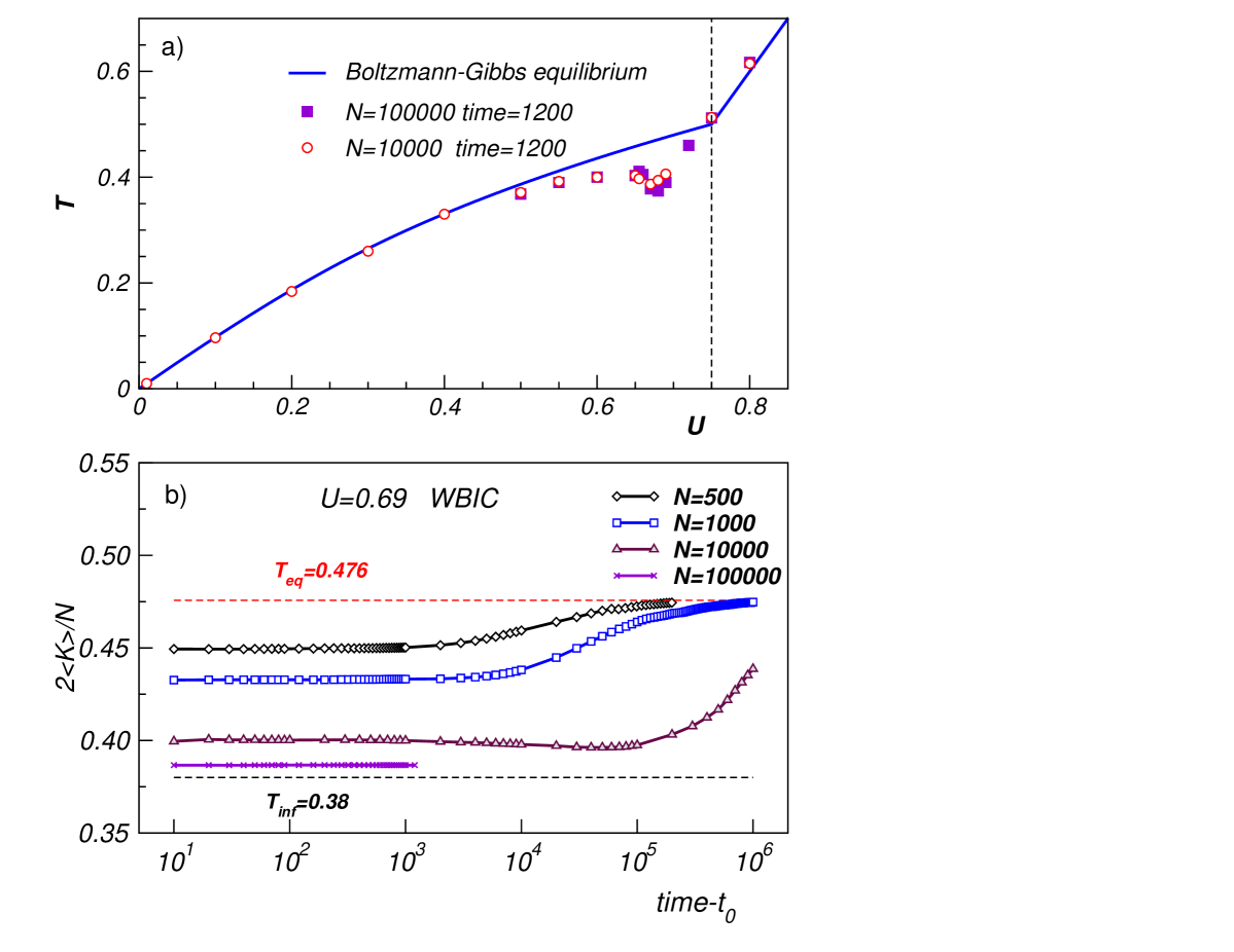
FIG. 1.: (a) We show the temperature T, calculated by taking the average kinetic energy per particle $2<K>/N$ , and the energy density $U=0.69$ for HMF systems of different sizes N=10000 (open circles) and N=100000 (squares). For comparison the equilibrium caloric curve is also shown as full line. The numerical simulations were initialized considering water bag initial conditions. The points are taken after a short time, t=1200, see text. The dashed line indicates the critical point. (b) We show the temperature time evolution for different N values. The initial part has been subtracted $(t_{0}=100)$. We report also the equilibrium temperature $T_{eq}$ (upper red dashed line) and $T_{\infty}$ the temperature to which the QSS tend for infinite size (bottom black dashed line).

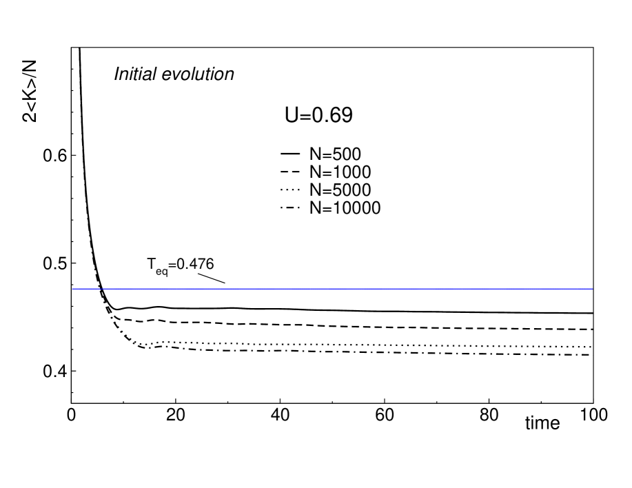
FIG. 2.: Initial time evolution of the quantity $2<K>/N$ for the HMF model. The numerical simulations correspond to different N sizes at $U=0.69$.

In fig.2 we show the initial time evolution of $2<K>/N$ to display the fast collapse of the initial condition to the metastable regime. We start our simulations by considering the so-called water-bag initial conditions , i.e. putting all the angles at zero and distributing the total energy uniformly over the momenta. The figure shows that there is a rapid evolution, which is not size-dependent, towards the QSS state. In ref. [10], we have also checked that these simulations are not affected by the numerical accuracy of the integration scheme used. This is certainly true in the range explored, with a relative error $10^{-7}<\Delta E/E<10^{-3}$, and demonstrates the robustness of these metastable QSS against small perturbations . At this point, it is interesting to calculate the specific heat in correspondence of this slow relaxation in the energy region below the critical point. The specific heat can be calculated from the fluctuations of kinetic energy, by using the microcanonical formulas derived in the 60’s by Lebowitz, Percus and Verlet (LPV formula) [18], i.e.

$$C_{V}={1\over 2}\left[1-2\left({\Sigma\over T}\right)^{2}\right]^{-1}$$ (4)

T being the microcanonical temperature and $\Sigma$ the kinetic energy microcanonical fluctuation. A second alternative is another formula which was derived more recently by Pearson, Haliciouglu and Tiller (PHT formula) [19]. The latter should be more precise, because it takes into account finite-size effects and is given by

$$C_{V}=\left[2<K><K>^{-1}+N(1-<K><K>^{-1})\right]^{-1}.$$ (5)

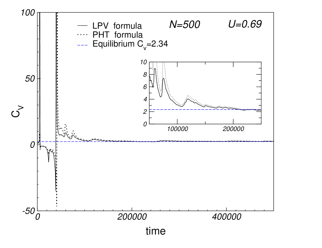
FIG. 3.: Specific heat calculations for the HMF model as a function of time in the case N=500 and U=0.69. The two different formulas discussed in the text, LPV formula (4) and PHT formula (5), are compared in the plot and in the inset magnification. The figure shows a very similar time evolution and a nice convergence for long times to the correct positive equilibrium value, indicated by the dashed line.

We report in fig.3 the specific heat calculated according to the eqs. (4) and (5) for N=500 and U=0.69. The figure shows a very similar time evolution for both formulas: after some oscillations, in which the specific heat is negative, both numerical simulations converge towards the same correct equilibrium positive value [16], also indicated as a dashed line. Let us now focus our attention on the transient regime, where the specific heat is negative. We have found that, in the transient QSS regime, the system does not show a Gaussian velocity probability distribution, while for longer integration times, when the system finally relaxes

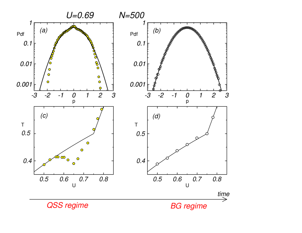
FIG. 4.: Caloric curves and velocity pdfs for the HMF model in the QSS regime and in the BG equilibrium regime for N=500.

to the equilibrium temperature, the velocity probability distribution (pdf) is perfectly Gaussian [10]. This result is nicely illustrated in fig.4. There we plot the numerical simulations for the caloric curve and the velocity pdfs both in the transient case, yellow circles in panels (c) and (a), and in the equilibrium case, white circles in panels (d) and (b). A back-bending of the HMF caloric curve in the transient regime clearly coincides with a non-Gaussian shape of the velocity pdf. In particular pdf tails are missing and slow decaying velocity correlations are present. One can also show that the velocity pdfs are frozen in this anomalous distribution for all the duration of the metastable regime. This result can be easily understood since the force, which each spin feels, is almost zero in the QSS regime. In fact the force on the single spin is given by the formula $F_{i}=-M_{x}sin\theta_{i}+M_{y}cos\theta_{i}$, where $M_{x}$ and $M_{y}$ are the components of the magnetization vector. Thus being $M^{2}=0$ in the QSS regime, it follows that also $F_{i}=0$ . The system is attracted by the QSS state and then remains in a frozen state. Why it then relaxes to the BG equilibrium? The answer is simple. If the system size is finite, the magnetization is not exactly zero, a small noise ($O\sim{1\over\sqrt{N}}$) always exists and this is responsible for the final relaxation to the BG equilibrium regime. The bigger the size, the smaller is the noise and thus the longer is the lifetime of the QSS state as numerically found [10]. This fact implies the interesting result that, if one inverts the order of the limits, i.e. takes first the infinite size limit instead of the infinite time limit, the noise is perfectly zero and the system remains trapped in the QSS state for ever. In [10] we have shown that the formalism proposed by Tsallis [8,9] seems to explain the shape of the velocity pdfs.

4 CONCLUSIONS

Summarizing,we have shown an example of a nonextensive system where a negative specific heat is found in correspondence to quasi-stationary states (QSS) and non-Gaussian velocity pdfs. This result which has been recently confirmed also in other long-range interacting models such as self-gravitating systems [7,12] and modified Lennard-Jones potentials [13] is due to the nonextensivity nature of the system into exam [14]. This fact is a serious warning for a straightforward claiming of a standard equilibrium first-order phase transition in nuclear fragmenting systems. Although some sort of equilibration seems to be reached in multifragmentation, it is not certain whether this corresponds to a complete relaxation. We stress the fact that the temperature deviation from its equilibrium value, we have discussed so far, is only of the order of 10% ! In this respect more detailed investigations should be done in order to further clarify the general theoretical scenario for nonextensive systems. But also more precise experimental data are very welcome and could be extremely useful to understand deeper the intriguing nature of phase transitions in finite systems, a field surely at the frontier of modern statistical mechanics.

REFERENCES

[1] D.H.E. Gross, Microcanonical thermodynamics: phase transitions in small systems , Lecture Notes in Physics, Springer-Verlag Heidelberg 2001 and refs therein. See also the proceedings of this workshop.

[2] P. Chomaz and F. Gulminelli, Nucl. Phys. A 647 (1999) 153

[3] M.D’Agostino et al, Phys. Lett. B A473 (2000) 219.

[4] M. Schmidt et al. Phys. Rev. Lett. 86 (2001) 1191.

[5] K. Huang, Statistical mechanics , Wiley (1987).

[6] J. Barrè, D. Mukamel, S. Ruffo, Phys. Rev. Lett. 87 (2001) 030601.

[7] A. Torcini, M. Antoni, Phys. Rev. E 89 (1999) 2746.

[8] C. Tsallis, J.Stat. Phys. 52 (1988) 479.

[9] For an updated review of this generalized statistics see the proceedings of the conference NEXT2001 published in Physica A 305 (2002). An updated reference list is also available at http://tsallis.cat.cbpf.br/biblio.htm

[10]V.Latora and A. Rapisarda, Nucl. Phys. A 681 (2001) 406c; V. Latora, A. Rapisarda and C. Tsallis, Phys. Rev. E 64 (2001) 056134 and Physica A 305 (2002) 129.

[11] C.Tsallis, B.J.C. Cabral, A. Rapisarda and V. Latora, [cond-mat/0112266] submitted to Phys. Rev. Lett.

[12] Sota et al, Phys. Rev. E 64 (2001) 05613; A. Taruya, M. Sakagami, Physica A (2002) in press [cond-mat/0107494].

[13] E.P. Borges and C. Tsallis, Physica A 305 (2002) 148.

[14] A. Campa, A. Giansanti, D. Moroni, Physica A 305 (2002) 137.

[15] M. Antoni and S. Ruffo Phys. Rev. E 52 (1995) 2361.

[16] V. Latora, A. Rapisarda and S. Ruffo, Phys. Rev. Lett. 80 (1998) 698, Physica D 131 (1999) 38 and Phys. Rev. Lett. 83 (1999) 2104.

[17] C. Anteneodo and C. Tsallis, Phys. Rev. Lett. 80 (1998)5313; A. Campa, A. Giansanti, D. Moroni and C.Tsallis, Phys. Lett. A 286 (2001) 251.

[18] J.L. Lebowitz, J.K. Percus and L. Verlet, Phys. Rev. A 153 (1967) 250.

[19] E.M. Pearson, T. Halicioglu and W.A. Tiller Phys. Rev. A 32 (1985) 3030.