Abstract

Starting from a gauge formalism of $\rho$ mesons, pions and baryons we evaluate the $\rho$ coupling to the nucleon, including the direct coupling provided by the Lagrangians, plus contributions from loops with the virtual pion cloud. We find a contribution to the magnetic $\rho$ coupling to the nucleon from pionic loops of the same size as the direct coupling, which is, however, still small compared to the empirical values. This finding goes in line with chiral formulations of the strong interaction of mesons at low energies where, unlike the scalar mesons which are mostly built of a pion (kaon) cloud, the $\rho$ meson stands as a genuine QCD state with intrinsic properties not tied to those of the pion cloud.

1 Introduction

The $\rho$ coupling to the nucleon has been the subject of permanent attention from different points of view. The $\rho$ exchange plays an important role in the nucleon-nucleon interaction at intermediate energies [1] and the strength of the tensor interaction is particularly large, about twice the value given by the vector meson dominance hypothesis (VMD). The determination of this coupling was done in [2] using dispersion relations and has been reconfirmed with posterior analysis along the same lines [3]. The strength of the tensor coupling found in [2, 3] finds also support from the values of the mixing parameter, $\epsilon$, at energies of the nucleons around or bigger than 200 MeV [4]. Attempts to describe this deviation from VMD have been done from different perspectives. In [5] an analysis using a topological chiral model concluded that the strong tensor coupling could be described semiquantitatively in a two phase model with half and half fractioning of charge and baryon number between the core and the soliton cloud. A color dielectric model was used in [6] concluding that the ratio $\kappa_{\rho}/\kappa_{v}$ was bigger than one. QCD sum rules have also been used in [7], and more recently in [8] where the tensor coupling is also found big and compatible with empirical determinations. Relativistic quark models were used to obtain also the $\rho NN$ coupling in [9]. The chiral quark models [10, 11] were also used to obtain the vector and tensor coupling in [12, 13], assuming that they come solely from the coupling of the $\rho$ to the pion cloud of the nucleon and determining the radius of the bag to reproduce the empirical results. In one way or another all these works come to confirm the important role of the pion cloud in these couplings.

However, stimulated by the interest in determining the renormalization of the $\rho$ properties in the nuclear medium, much work has been done recently [14, 15, 16, 17, 18] which make a revision of the problem timely. There has also been progress in another front concerning the $\rho$ meson. Indeed, Chiral Perturbation Theory, ($\chi PT$), as an effective theory of the underlying QCD, has emerged as a useful tool to deal with hadronic interactions at low and intermediate energies. For the meson meson interaction the basic dynamics is contained in the lowest and second order Lagrangians of Gasser and Leutwyler [19, 20]. One important step forward in the understanding of the content of these Lagrangians was done in [21] where it was found that the parameters of the second order Lagrangian could be generated by the explicit exchange of resonances, particularly the vector mesons. Another step forward was subsequently given in [22] where the lowest order chiral Lagrangian, together with the exchange of vector and scalar mesons suggested in [21], were used to study the meson meson interaction, implementing unitarity via the N/D method. The result of this work was that, while the coupling of the vector mesons to the pseudoscalar mesons was essential to reproduce the data, the coupling of the scalars was compatible with zero. Yet, the scalar mesons were generated within the unitary approach simply from the multiple scattering of the mesons driven by the interaction accounted for by the lowest order Lagrangian. These mesons are hence dynamically generated in this approach, contrary to the vector mesons which qualify as genuine mesons. This classification can also be linked to arguments of the large $N_{c}$ limit in QCD. Indeed, loops are subleading in the $N_{c}$ counting, and consequently in the large $N_{c}$ limit the scalar mesons would disappear while the formerly called genuine mesons would survive, hence giving extra meaning to the concept of genuine and dynamically generated mesons [22, 23, 24, 25].

This distinction is hence more than semantics and has practical repercussions. Indeed, since the lowest of the scalar mesons, the $\sigma$, is built up here from the meson meson interaction, consistency with this picture demands that the coupling of a $\sigma$ to the nucleon is simply done by coupling the interacting meson pair to the nucleon and this is what was done in [26]. However, since the $\rho$ meson qualifies as one of the genuine mesons, its coupling to the nucleon does not have to come from just the pion cloud within this approach and, indeed, the effective Lagrangians used in [14, 15, 16, 17, 18] contain a direct coupling of the $\rho$ to the nucleon.

With this picture in mind, and within the philosophy of these effective Lagrangians, it is still proper to ask which is the contribution to the $\rho NN$ coupling from the mesonic loops in the perturbative expansion.

There is also another new element in the present evaluation since the findings of the lattest references [14, 15, 16, 17, 18] have also shown the importance of vertex corrections, linked to the underlying gauge structure of the Lagrangians, which were overlooked in the previous determinations of the meson cloud contributions to the $\rho$ couplings. All these findings introduce new elements in the evaluation of the vector and tensor couplings of the $\rho$ to the nucleon and the purpose of the present work is to give a new look to the problem from this modern perspective.

2 Model for the $\rho NN$ coupling

We shall calculate the nucleon coupling to the $\rho$ meson based on the chiral Lagrangian for the pion and nucleon. The basic couplings of the pion and nucleon to the $\rho$ meson are introduced by imposing the gauge theory for vector meson on the chiral Lagrangian. In the gauge theory for vector meson, this particle is considered as a gauge boson of an implicit gauge symmetry, which was originally suggested by Sakurai [27] with the vector meson dominance hypothesis, where it mediates all hadronic interactions. Later on, Bando et al. [28] developed this idea to the hidden local gauge theory of the non-linear sigma model. As we shall see, at tree level, the gauge condition of the vector meson on the chiral Lagrangian gives only the vector coupling of the $\rho NN$ vertex, since the tensor coupling itself is free from the gauge constraint. Therefore, in absence of direct tensor contributions, the tensor coupling is generated through pion-loop contributions. The study of such contributions is the aim of this paper.

Let us start by considering the elementary $\rho NN$ vertex. According to the construction of the gauge theory, the direct coupling of a hadron $h$ to the $\rho$ meson is constructed replacing the derivative by the associated covariant derivative with the gauge symmetry :

$$\partial_{\mu}h(x)\rightarrow D_{\mu}h(x)=\partial_{\mu}h(x)+ig_{\rho}[h(x),V^{a}]\rho^{a}_{\mu}$$ (1)

where $V^{a}$ is the generator of the gauge symmetry of the $\rm SU(2)$ isospin space and the hadronic charge $g_{\rho}$ is given as a universal constant in all hadrons.

For the nucleon, since under the isospin rotation it is transformed as the fundamental representation: $[V^{a},\psi_{N}]=-{1\over 2}\tau^{a}\psi_{N}$, the covariant derivative for the nucleon is written as

$$D_{\mu}\psi_{N}=(\partial_{\mu}+i{g_{\rho}\over 2}\vec{\tau}\cdot\vec{\rho}_{\mu})\psi_{N}$$ (2)

where $\tau^{a}$ is the Pauli matrix for the isospin. Thus, the replacement on the kinetic term of the nucleon, $\bar{\psi}_{N}i\partial/\psi_{N}\rightarrow\bar{\psi}_{N}i{D/}\psi_{N}$, gives the direct coupling of the $\rho$ meson to the nucleon:

$${\cal L}_{\rho NN}=-{g_{\rho}\over 2}\bar{\psi}_{N}\gamma^{\mu}\vec{\rho}_{\mu}\cdot\vec{\tau}\psi_{N}$$ (3)

Figure 1: The direct $\rho NN$ coupling.

The Lagrangian (3) contributes the vertex shown in fig.1 as

$${-it}_{\rho NN}^{\rm direct}=-i{g_{\rho}\over 2}\tau^{a}\gamma\cdot\varepsilon^{*}\ ,$$ (4)

where $\varepsilon_{\mu}$ is the polarization vector of $\rho$, and $a$ is the isospin index of the $\rho$ meson. In general, the vertex function of the $\rho NN$ coupling is written in terms of two Lorentz independent functions $G^{V}$ and $G^{T}$:

$$-it_{\rho NN}=i\left(G^{V}(q^{2})\gamma^{\mu}+{G^{T}(q^{2})\over 2iM_{N}}\sigma^{\mu\nu}q_{\nu}\right)\varepsilon_{\mu}^{*}\tau^{a}\ ,$$ (5)

where $q$ is the outgoing momentum of the $\rho$. From eq. (4) the vertex functions $G^{V}$ and $G^{T}$ at tree level are obtained with the result

$$G^{V}_{\rm tree}=-{g_{\rho}\over 2}\ ,\hskip 14.22636ptG^{T}_{\rm tree}=0$$ (6)

while empirically one has

$$G^{V}_{\rm emp.}=2.9\pm 0.3,\hskip 14.22636ptG^{T}_{\rm emp.}=18\pm 2$$ (7)

In the Lagrangian language, the tensor part is written as

$${\cal L}^{\rm tensor}_{\rho NN}=-{G^{T}\over 2M_{N}}\bar{\psi}_{N}F^{\mu\nu}_{a}\sigma_{\mu\nu}{\tau^{a}\over 2}\psi_{N}$$ (8)

with the field strength tensor of the rho meson $F_{\mu\nu}^{a}=\partial_{\mu}\rho_{\nu}^{a}-\partial_{\nu}\rho_{\mu}^{a}-g_{\rho}\epsilon_{abc}\rho_{\mu}^{b}\rho_{\nu}^{c}$. The Lagrangian of eq. (8) itself is invariant under the gauge transformation. Therefore the value of the coefficient $G^{T}$ is free from the constraint of the gauge theory. Here we would like to calculate $G^{T}$ from pion-loop contributions as the pion cloud without introducing any direct tensor couplings.

For later convenience we work with the Breit frame, that is $q^{0}=0$, $p_{i}=\vec{q}/2$ and $p_{f}=-\vec{q}/2$, and also use the non-relativistic form. Then eq. (5) is written as

$$-it_{\rho NN}=\left(iG^{E}(q)\varepsilon^{0}-{G^{M}(q)\over 2M_{N}}(\vec{\sigma}\times\vec{q})\cdot\vec{\varepsilon}\right)\tau^{a}\ ,$$ (9)

with

$$G^{E}(q) = G^{V}(q)$$ (10)

$$G^{M}(q) = G^{T}(q)+G^{V}(q)\ .$$ (11)

In order to include the contribution from the pion cloud, we calculate the indirect coupling of the $\rho$ meson to the nucleon shown in fig.2 a). Since this diagram is one-loop, we also consider other one-loop diagrams shown in fig.2 for consistency of the loop expansion. As intermediate baryons in the loops, which can be excited by the pion, we consider both nucleon and $\Delta$. The loop corrections do not contribute to $G^{E}$ at $q=0$ due to the Ward-Takahashi identity.

The $\rho\pi\pi$ coupling is introduced by the gause theory for vector meson in the same way as the nucleon case. With the isospin rotation for pions $[V^{a},\pi^{b}]=-i\epsilon^{abc}\pi^{c}$, we obtain the covariant derivative for the pion:

$$D_{\mu}\pi^{a}=\partial_{\mu}\pi^{a}+g_{\rho}\epsilon_{abc}\pi^{b}\rho^{c}_{\mu}$$ (12)

and, then, from the replaced kinetic term ${1\over 2}D_{\mu}\vec{\pi}\cdot D^{\mu}\vec{\pi}$, we obtain the $\rho\pi\pi$ vertex :

$${\cal L}_{\pi\pi\rho}=-g_{\rho}(\vec{\pi}\times\partial^{\mu}\vec{\pi})\cdot\vec{\rho}_{\mu}$$ (13)

With this Lagrangian we can calculate the decay width of the $\rho$ meson decaying to two pions, which gives $g_{\rho}=-6.14$. The sign is given by comparing to the standard $\rho$ coupling to pions in the chiral tensor formalism [21], which provides the equivalence $g_{\rho}=-m_{\rho}G_{V}/f^{2}$, where $G_{V}$ is the parameter appearing in the chiral resonance Lagrangians of ref. [21] providing the $\rho\pi\pi$ coupling.

For the $\pi N$ couplings, we use the chiral Lagrangian:

$${\cal L}_{\pi N}=-{g_{A}\over 2f}\bar{N}\partial/\gamma_{5}\vec{\pi}\cdot\vec{\tau}N-{1\over 4f^{2}}\bar{\psi}_{N}(\vec{\pi}\times\partial/\vec{\pi})\cdot\vec{\tau}\psi_{N}+\cdots\ ,$$ (14)

where $\cdots$ denotes terms with multiple pions which do not enter the present calculation. In eq. (14) $g_{A}$ is the axial charge of the nucleon, $g_{A}=1.26$. In alternative formulations $g_{A}$ appears as $D+F$, with $D$ and $F$ the two $SU(3)$ coefficients for the semileptonic decay of hyperons, or through $g_{A}/2f\equiv f_{\pi NN}/m_{\pi}$. The gauge theory for vector meson introduces the $\pi\rho NN$ coupling through the replacement of the derivative by the covariant derivative (12):

$${\cal L}_{\pi\rho N}={g_{A}g_{\rho}\over 2f}\bar{N}(\vec{\rho}_{\mu}\times\vec{\pi})\cdot\vec{\tau}\gamma^{\mu}\gamma_{5}N+{g_{\rho}\over 4f^{2}}\bar{\psi}_{N}\gamma^{\mu}(\vec{\pi}\cdot\vec{\pi}\vec{\rho}_{\mu}\cdot\vec{\tau}-\vec{\pi}\cdot\vec{\rho}_{\mu}\vec{\pi}\cdot\vec{\tau})\psi_{N}+\cdots$$ (15)

The first terms of eqs.(14) and (15) give the $\pi NN$ and $\pi\rho NN$ vertices. After the non-relativistic reduction we have

$$-it_{\pi NN} = -{g_{A}\over 2f}\vec{q}\cdot\vec{\sigma}\ \tau^{a}$$ (16)

$$-it_{\pi\rho NN} = i{g_{A}g_{\rho}\over 2f}\vec{\sigma}\cdot\vec{\varepsilon}\ \epsilon_{abc}\tau^{c}$$ (17)

where $a$ and $b$ are the isospin indices for $\pi$ and $\rho$, respectively, and $\vec{q}$ is the outgoing pion momentum.

For the $\Delta$ contribution, the introduction of $\pi N\Delta$ coupling is empirically performed through the replacement of the spin-isospin matrix $\vec{\sigma}$, $\vec{\tau}$ on the $\pi NN$ vertex by the spin-isospin transition matrices $\vec{S}$, $\vec{T}$:

$$-it_{\pi N\Delta}=-\left({f_{\pi N\Delta}\over f_{\pi NN}}\right){g_{A}\over 2f}\vec{q}\cdot\vec{S}\ T^{a}$$ (18)

where $(f_{\pi N\Delta}/f_{\pi NN})=2.13$. If we recall the introduction of the rho meson coupling through the replacement of eq. (12), the $\pi N\Delta$ coupling relates to the $\pi\rho N\Delta$ one. Therefore, in analogy with the introduction of the $\pi\rho NN$ coupling (17) from the $\pi NN$ vertex (16), we have

$$-it_{\pi\rho N\Delta}=i\left({f_{\pi N\Delta}\over f_{\pi NN}}\right){g_{A}g_{\rho}\over 2f}\vec{S}\cdot\vec{\varepsilon}\ \epsilon_{abc}T^{c}$$ (19)

For the $\rho\Delta\Delta$ coupling, we use the gauge theory for vector mesons again. The covariant derivative for the delta baryon is given in the relativistic form with the Rarita-Schwinger field for the spin $3/2$ fermion as

$$D_{\mu}\psi_{\Delta,\nu}=\partial_{\mu}\psi_{\Delta,\nu}+ig_{\rho}\vec{T}_{\Delta}\cdot\vec{\rho}_{\mu}\psi_{\Delta,\nu}$$ (20)

where $T_{\Delta}$ is the isospin $3/2$ matrix, which is normalized so that $T^{3}_{\Delta 11}=3/2$. The kinetic term for the $\Delta$ with the covariant derivative, which is written as $\bar{\psi}_{\Delta,\mu}i{D/}\psi^{\mu}_{\Delta}$, gives the direct coupling of the $\Delta$ to the $\rho$ meson. Similarly to the nucleon case, there exists a tensor coupling free from the gauge constraint. After including the tensor coupling and the non-relativistic reduction, the $\rho\Delta\Delta$ vertex is written as

$$-it_{\rho\Delta\Delta}=\left(-ig_{\rho}\varepsilon^{0}-{G_{\Delta}^{M}\over 2M_{N}}(\vec{S}_{\Delta}\times\vec{q})\cdot\vec{\varepsilon}\right)T_{\Delta}^{a}$$ (21)

where $S_{\Delta}$ is the same matrix as the isospin matrix $T_{\Delta}$ but for spin space, and $G^{M}_{\Delta}$ is a free parameter. Here we assume that the magnetic coupling of the direct $\rho\Delta\Delta$ is scaled to that of the $\rho NN$ according to the quark model [29], which is

$$G^{M}_{\Delta}={4\over 5}G^{M}_{N}$$ (22)

The derivation is written in Appendix A. If the direct tensor term is not included, the magnetic coupling comes from the vector term and we obtain $G^{M}_{\Delta}={4\over 3}{M_{N}\over M_{\Delta}}G^{M}_{N}$.

For the $\rho N\Delta$ coupling, the vector coupling is not allowed due to the spin symmetry, thus, only the magnetic coupling is allowed and given as

$$-it_{\rho N\Delta}=\left(-{G_{N\Delta}^{M}\over 2M_{N}}(\vec{S}\times\vec{q})\cdot\vec{\varepsilon}\right)T^{a}$$ (23)

with the quark model result

$$G^{M}_{N\Delta}={6\over 5}\sqrt{2}G^{M}_{N}$$ (24)

3 One loop contributions

The evaluation of the tree level diagram with a contact $\rho NN$ interaction from the Lagrangian of eq. (3) contributes to the $G^{E}_{\rho NN}$ term, providing a value $G^{E}_{\rho NN}=\frac{M_{\rho}G_{V}}{2f^{2}}F_{\rho}(\vec{Q}=\vec{0})$=3.07, which is already a very good value when compared to the experimental one, $G^{E}_{\rho NN}=2.9\pm 0.3$ ($F_{\rho}(\vec{Q})$ is the $\rho$ form factor, defined in Appendix B). However, this is the only contribution to $G^{M}_{\rho NN}$ , which has an empirical value around 21. We want to see how much of the magnetic strength can be generated through loop contributions. In this section we perform the one loop calculation, which comes from the diagrams shown in figure 2 plus other time orderings. In all of them we assume the external nucleon lines to be protons.

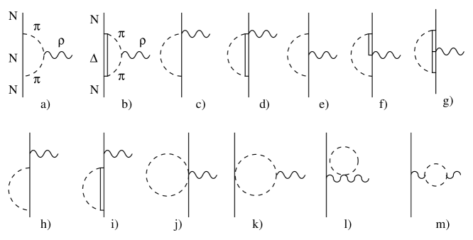
Figure 2: One loop diagrams evaluated.

The contribution of each of these diagrams to $G^{E}_{\rho NN}$ and to $G^{M}_{\rho NN}$ is given in Appendix B. We discuss here in more detail the calculations and the results obtained. In what follows we present results calculated with the form factors for $\pi$ and $\rho$ given in eq. (45) and we take $g_{A}=1.26$ and $f=93$ MeV.

In diagram a) the pions are a $\pi^{+}\pi^{-}$ pair since the $\pi^{0}\pi^{0}$ pair does not couple to the $\rho^{0}$, being the intermediate nucleon a neutron. The evaluation of this diagram is straightforward and gives the values $G^{E}_{\rho NN}(\vec{q}=\vec{0})=1.64$ and $G^{M}_{\rho NN}(\vec{q}=\vec{0})=4.42$. The calculation of diagram b) is analogous, once the spin and isospin factors arising from eq. (50) of Appendix B are taken into account. It gives $G^{E}_{\rho NN}(\vec{q}=\vec{0})=-1.11$ and $G^{M}_{\rho NN}(\vec{q}=\vec{0})=1.44$. As we can see, the contributions of these two diagrams to $G^{E}_{\rho NN}$ have opposite sign, and therefore there is an important cancellation between them, while the contributions to $G^{M}_{\rho NN}$ have the same sign.

The other diagrams to be considered, except for diagram k), contain vertices in which the $\rho$ is coupled directly to a nucleon leg. In all these cases we have multiplied the result provided by the expressions given in Appendix B by the corresponding $F_{\rho}(\vec{Q})$ form factor, defined in eq. (45). The results given in Appendix B for diagram c) accounts for the diagram represented in c) of figure 2 but also for the one with the $\rho$ meson attached to the lower vertex instead of the upper one. In these vertices the pions are charged. Their contribution to $G^{E}_{\rho NN}$ is of order ${\cal O}(1/M)$ and is not considered here. The contribution to $G^{M}_{\rho NN}$ is found to be $G^{M}_{\rho NN}(\vec{q}=\vec{0})=-1.90$. In the case of diagram d) there are two more diagrams contributing since we can have $p\pi^{-}\Delta^{++}$, $\rho p\pi^{-}\Delta^{++}$ vertices. We obtain from these diagrams $G^{M}_{\rho NN}(\vec{q}=\vec{0})=-0.55$, being the contribution to $G^{E}_{\rho NN}$ of ${\cal O}(1/M)$ as in the previous case.

In diagrams e), f) and g) we have the $\rho NN$, $\rho N\Delta$ and $\rho\Delta\Delta$ vertices. The contributions to $G^{E}$ and $G^{M}$ of these diagrams are written in Appendix B, where we have taken into account the quark model based relations between $G^{M}$, $G^{M}_{\Delta}$ and $G^{M}_{N\Delta}$ of Appendix A. Diagram e) accounts actually for two diagrams, one with an intermediate $p$ and another one with an intermediate $n$. The evaluation of these diagrams is simple and gives $G^{E}_{\rho NN}(\vec{q}=\vec{0})=-0.41$ and $G^{M}_{\rho NN}(\vec{q}=\vec{0})=0.14$. In the case of diagrams f) and g) we have to take into account that they correspond to more diagrams than in the case of diagram e) since we can have an intermediate $\Delta^{++}$ in addition to $\Delta^{+}$ and $\Delta^{0}$. In the evaluation of diagram g) we need to apply the following relation:

$$S_{i}S_{\Delta j}S^{\dagger}_{k}=\frac{5}{6}\textrm{i}\epsilon_{ijk}-\frac{1}{6}\delta_{ij}\sigma_{k}+\frac{2}{3}\delta_{ik}\sigma_{j}-\frac{1}{6}\delta_{jk}\sigma_{i}$$ (25)

With this we get $G^{E}_{\rho NN}(\vec{q}=\vec{0})=2.77$ and $G^{M}_{\rho NN}(\vec{q}=\vec{0})=0.93$ from these diagrams. We find also that diagrams of type f) do not contribute to $G^{E}_{\rho NN}$, and they provide a contribution to $G^{M}$ of $G^{M}_{\rho NN}(\vec{q}=\vec{0})=1.40$.

The next diagrams that we have considered, h) and i), correspond to the wave function renormalization. Their evaluation is straightforward, and their effect is taken into account by multiplying the tree level contribution by $(1+\partial\Sigma/\partial k^{0}$) (see Appendix B). Finally, diagrams j) and k) cancel at $\vec{q}=\vec{0}$ (see Appendix B), and therefore we do not consider them here. Diagrams c) and d), containing the vertex corrections, have been neglected in the evaluation of $G^{E}$ because they are of order $1/M$ of the rest of the diagrams and terms of this order (recoil corrections) have been omitted in the $\pi NN$, $\pi N\Delta$ and $\pi\Delta\Delta$ vertices. However, we have evaluated numerically the contribution of these terms, and although individually they are not too small we find a very good cancellation between the terms involving a nucleon or a $\Delta$ propagator, thus justifying altogether the neglecting of all these terms.

We should also point out that we have not included diagrams m) where the $\rho$ couples directly to the nucleon and there is a selfenergy insertion in the $\rho$ corresponding to a two pion loop , or similarly diagrams l), where a tadpole of a pion loop is attached to the $\rho$ propagator. Such terms, as shown in [18, 30] go into the renormalization of the $\rho$ mass and width.

In table 1 we summarize the results obtained here for $G^{E}$ and $G^{M}$ at $\vec{q}=\vec{0}$.

	tree	a)	b)	c)	d)	e)	f)	g)	h)	i)	total
$G^{E}$	3.07	1.64	-1.11	–	–	-0.41	–	2.77	-1.23	-1.66	3.07
$G^{M}$	3.07	4.42	1.44	-1.90	-0.55	0.14	1.40	0.93	-1.23	-1.66	6.05

Table 1: Different contributions to $G^{E}$ and $G^{M}$ at $\vec{q}=\vec{0}$.

It is worth noting that the different loop contributions approximately cancel with the wave function renormalization (see table 1) in $G^{E}(\vec{q}=\vec{0})$. The cancellation appears from diagrams a), e), h) as a block, which are the terms containing intermediate nucleon propagators, and from diagrams b), g) and i) which contain the $\Delta$ propagators. This cancellation can be found analytically from the expressions in Appendix B at $\vec{q}=\vec{0}$ if we include only one factor $M/E$ in the set of baryon propagators to keep at the same order of a non-relativistic expansion.

The interesting thing to see in table 1 is that the loops provide a sizeable contribution to $G^{M}(\vec{q}=\vec{0})$ which has now a value of 6.05, about double the one from the tree level. This number is still small compared to the empirical value of $G^{M}\sim 21$, and the discrepancy should be attributed to non-perturbative effects.

In order to estimate the uncertainties we have changed the value of the form factor parameter for the pion and the value of $D+F$. If we use for instance $D+F=2ff_{\pi NN}/\mu$ instead of $D+F=g_{A}$ we obtain $G^{M}(\vec{q}=\vec{0})=6.39$. If we change $\Lambda_{\pi}$ from 0.9 GeV to 1.2 GeV we obtain $G^{M}(\vec{q}=\vec{0})=6.41$. The results obtained by changing the parameters reasonably indicate that the uncertainties in the theoretical calculation are around as less than 10%.

Finally, in figure 3 we plot the results for the $\vec{q}$ dependence (form factor) of $G^{E}(\vec{q})$ and $G^{M}(\vec{q})$. They are compared with the empirical form factor, assuming the same normalization at $\vec{q}=\vec{0}$. For the $\vec{q}$ dependence of our results we sum the tree level contribution multiplied by the empirical form factor and the loop contributions evaluated here. We can see that our calculation falls down faster than a monopole form factor at low energies, perticularly the tensor part.

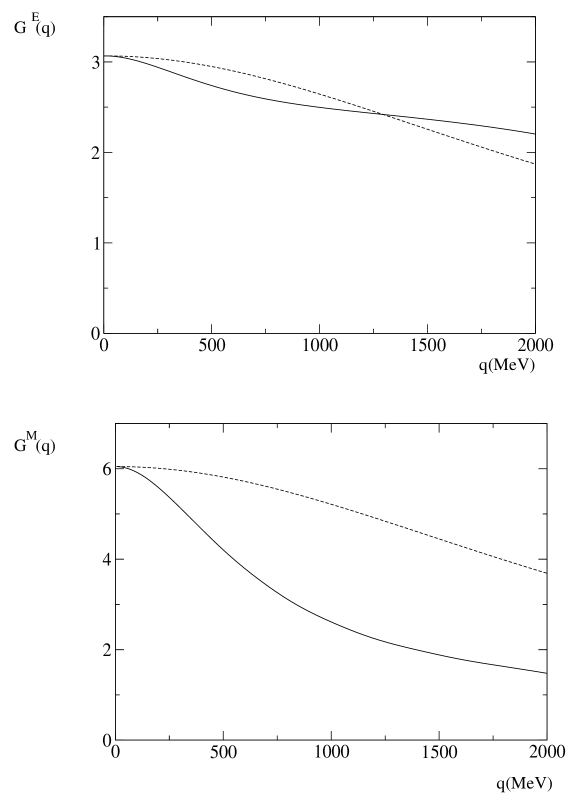
Figure 3: Comparison between the theoretical form factors (solid line) and the empirical form factors as the one given in Appendix B (dashed line).

4 Considerations on gauge invariance

Although the procedure followed with the Feynman diagrams used would fulfill gauge invariance, our introduction of the explicit form factors of Appendix B would break it. This is a well known fact and in the literature there have been many attempts to restore gauge invariance in the presence of form factors [16, 31, 32].

Since our main concern is to show the contribution of loops to the magnetic coupling (at $\vec{q}=\vec{0}$) or to $G^{E}$ and $G^{M}$ at moderate values of $\vec{q}$, rather than embarking in some of the procedures to restore gauge invariance as quoted above, we shall make a study here of why and how gauge invariance is broken and this will give us an idea for which values of $\vec{q}$ our procedure still satisfies gauge invariance and hence makes the results credible. Let us take the contribution from all loop diagrams from a) to g) in fig. 2 with an incoming nucleon momentum $p$ and an outgoing nucleon momentum $p+q$, and call their contribution to -i$t^{\mu}$:

$$-\textrm{i}\Delta t^{\mu}\equiv\textrm{i}\Delta G^{V}(q)\gamma^{\mu}+\frac{G^{T}(q)}{2\textrm{i}M_{N}}\sigma^{\mu\nu}q_{\nu}$$ (26)

A general test of gauge invariance can be given by the Ward identities which establish in the $\rho NN$ case [16]

$$-\textrm{i}\Delta t^{\mu}(q)q_{\mu}=\textrm{i}\frac{g_{\rho}}{2}\left(\Sigma(p+q)-\Sigma(p)\right)$$ (27)

where $\Sigma(p)$ is the nucleon self-energy. Eq.(27) implies

$$\textrm{i}\Delta G^{V}(q)\gamma^{\mu}q_{\mu}=\textrm{i}\frac{g_{\rho}}{2}\left(\Sigma(p+q)-\Sigma(p)\right)$$ (28)

which should be valid for any value of $p$ and $q$ even if the nucleons and the $\rho$ are off shell. By chosing $p^{0}=M_{N}$, $\vec{p}=\vec{0}$ and arbitrary $q^{0}$, $\vec{q}$, which is a sufficiently general situation, we have:

$$\textrm{i}\Delta G^{V}(q)\gamma^{\mu}q_{\mu}=\textrm{i}\frac{g_{\rho}}{2}\left(\Sigma(q^{0}+M_{N},\vec{q})-\Sigma(M_{N},\vec{0})\right)$$ (29)

where in the non relativistic expansion which we are using $\Sigma(p)$ is just a number. We now evaluate the matrix element of the first member of eq. (28) between the spinors $\bar{u}(\vec{p}+\vec{q})$ and $u(\vec{p})$ in the same non-relativistic approximation. Then we obtain

$$\textrm{i}\Delta G^{V}\left(q^{0}-\frac{\vec{q}^{\textrm{ }2}}{2M_{N}}\right)=\textrm{i}\frac{g_{\rho}}{2}\left(\Sigma(q^{0}+M_{N},\vec{q})-\Sigma(M_{N},\vec{0})\right)$$ (30)

Let us now take $q^{0}$, $q$ small enough such that a Taylor expansion of $\Sigma$ can be done and we obtain

$$\textrm{i}\Delta G^{V}\left(q^{0}-\frac{\vec{q}^{\textrm{ }2}}{2M_{N}}\right)=\textrm{i}\frac{g_{\rho}}{2}\left(q^{0}\left.\frac{\partial\Sigma}{\partial q^{0}}\right|_{q^{0}=q=0}+\vec{q}^{\textrm{ }2}\left.\frac{\partial\Sigma}{\partial\vec{q}^{\textrm{ }2}}\right|_{q^{0}=q=0}\right)$$ (31)

which by means of the easily derivable relation

$$\left.\frac{\partial{\Sigma}}{\partial\vec{q}^{\textrm{ }2}}\right|_{q^{0}=q=0}=-\frac{1}{2M_{N}}\left.\frac{\partial\Sigma}{\partial q^{0}}\right|_{q^{0}=q=0}$$ (32)

leads to

$$\textrm{i}\Delta G^{V}\left(q^{0}-\frac{\vec{q}^{\textrm{ }2}}{2M_{N}}\right)=\textrm{i}\frac{g_{\rho}}{2}\left.\frac{\partial\Sigma}{\partial q^{0}}\right|_{q^{0}=q=0}\left(q^{0}-\frac{\vec{q}^{\textrm{ }2}}{2M_{N}}\right)$$ (33)

This requires (omitting higher orders $q^{0}$, $\vec{q}$) that

$$\left.\Delta G^{V}(q)\right|_{q^{0}=q=0}-\frac{g_{\rho}}{2}\left.\frac{\partial\Sigma}{\partial q^{0}}\right|_{q^{0}=q=0}=\left.\left(\Delta G^{E}+G^{E}_{tree}\frac{\partial\Sigma}{\partial q^{0}}\right)\right|_{q^{0}=q=0}=0$$ (34)

As we have noted in the former section, $\Delta G^{E}+G^{E}_{tree}\frac{\partial\Sigma}{\partial q^{0}}$ gives the contribution to $G^{E}(q)$ from the loop vertex functions of diagrams a) to g) of fig. 2, plus the contribution from the wave function renormalization (diagrams h), i) of fig. 2) which is given by the second term, $G^{E}_{tree}\frac{\partial\Sigma}{\partial q^{0}}$. Eq. (34) tells us that the contribution of all those terms to $G^{E}(0)$ is null, something that we had already found numerically even with the presence of form factors. It is not surprising that this should be the case because it should occur in the absence of form factors from a cancellation of the contribution of the different diagrams. Then at $q^{0}=q=0$ all these diagrams are multiplied by the same form factors and hence the cancellation also holds. Since eq. (34) is satisfied also in the case of form factors, then eq. (33), which is the statement of the Ward identities at moderate values of $q^{0}$ and $q$, also holds in the presence of form factors. However, the limits go beyond those where the Taylor expansion may hold. Indeed, as we stated above, the Ward identities in the absence of form factors would be fulfilled and if all the diagrams were multiplied in our case by the same form factors then the equality would still hold. However, this is the case only at $q^{0}=q=0$, because for finite $q$ we have in the loops $F_{\pi}^{2}(\vec{p})$ in some diagrams and $F_{\pi}(\vec{p})F_{\pi}(\vec{p}+\vec{q})$ in other diagrams, which are not the same. Also we have the $\rho NN$ form factor which does not appear in diagrams a) and b). Since the form factor is only operative for values of $|\vec{p}|$ of the order of the cut off $\Lambda$ or higher, demanding that the angle averaged value of $F_{\pi}(\vec{p})F_{\pi}(\vec{p}+\vec{q})$ be similar to $F_{\pi}^{2}(\vec{p})$, for instance, implies that $q$ should be small compared to the cut off scale $\Lambda$.

The former argument sets the scale of values of $q$ where gauge invariance would be violated. On the other hand the results of [32] using the gauge restoring Berends formalism or the plain application of form factors showed that the differences were not large even at values of $|\vec{q}|\sim 800$ MeV. All these things considered, one can reasonably say that up to values of $q\sim 500$ MeV the results evaluated here would be reliable.

5 Conclusions

We have evaluated the contributions to $G^{E}(\vec{q})$ and $G^{M}(\vec{q})$ for the coupling of the $\rho$ meson to the nucleon including direct couplings stemming from a gauge formulation of the theory and in addition we have included the contributions of the virtual meson cloud at one loop level. We regularize the loops by means of a form factor, introducing an effective cut off of the order of 1 GeV which is considered the natural scale. In addition to this cut off the space of the intermediate states is reduced to the nucleon and the $\Delta$. This means a regularization from two sources and the justification should be seen in the phenomenological success of such an approach in a large number of hadronic properties in the evaluation of chiral bag models [33].

What we find, as expected, is that $G^{E}(\vec{q}=\vec{0})$ does not change with respect to the tree level, because it is restricted by gauge conditions, but $G^{M}(\vec{q}=\vec{0})$, which has no such restrictions, is appreciably enhanced. However, this enhancement is still clearly insufficient to provide values close to the empirical one. This result seems to indicate that the magnetic coupling of the $\rho$ to the nucleon is of direct nature and cannot be attributed to loop corrections. The $\rho$, as a genuine QCD state [21], by contrast to the low energy scalar mesons [34], has also as a genuine property a strong magnetic coupling to the nucleon, the origin of which goes beyond the meson loop calculation which we have done. This is in contrast to the coupling of the $\sigma$ meson to the nucleon which, in correspondence to the nature of the $\sigma$ as a pion-pion rescattering resonance, could be obtained by coupling the meson cloud to the nucleons [26, 35].

On the other hand we observe that the loop contribution to the electric and magnetic form factors has a stronger $\vec{q}$ dependence than the one provided by the assumed empirical monopole form factor. This is due to the large extend of the pion cloud, which, due to the small mass of the pion, has a larger range than the genuine constituents (quarks) of the $\rho$ meson. This faster fall of the form factors, or, alternativelly the larger range of the coupling, should also have some repercussion in the part of the $NN$ interaction mediated by $\rho$ exchange.

Acknowledgments

One of us, D.J. wishes to acknowledge the hospitality of the University of Valencia where this work was done and financial support from the Ministerio de Educacion in the program Doctores y Tecnologos extranjeros. J. E. P. wishes to acknowledge support from Ministerio de Educación, Cultura y Deporte. This work is also partly supported by DGICYT contract number BFM2000-1326 and E.U. EURODAPHNE network contract no. ERBFMRX-CT98-0169.

Appendix A $G^{M}_{\Delta}$ and $G^{M}_{N\Delta}$ from the quark model

Here we explain the calculations of the $\rho\Delta\Delta$ and $\rho N\Delta$ couplings from the $SU(6)$ quark model. Now let us define the operator of the $\rho^{0}$ coupling to the $i$-th quark for $G_{M}$:

$$\hat{g}_{M}^{(i)}=-G^{M}_{(q)}{(\vec{q}\times\vec{\varepsilon})\cdot\vec{\sigma}_{(i)}\over 2m_{q}}\tau^{3}_{(i)}$$ (35)

with the light quark mass $m_{q}$ and an outgoing $\rho^{0}$ momentum $\vec{q}$. The $G^{M}$ for proton with up spin is calculated from the quark model as

$$\langle p\uparrow|\sum_{i=1}^{3}\hat{g}_{M}^{(i)}|p\uparrow\rangle=-{5\over 3}G^{M}_{(q)}{(\vec{q}\times\vec{\varepsilon})_{3}\over 2m_{q}}$$ (36)

Here we use $\langle p\uparrow|\sigma^{3}\tau^{3}|p\uparrow\rangle={5\over 3}$ and the $SU(6)$ flavor-spin symmetry for the nucleon wave function:

$$|N\rangle={1\over\sqrt{2}}(\phi_{MS}\chi_{MS}+\phi_{MA}\chi_{MA})$$ (37)

with, for the proton with the spin up,

$$\phi_{MS}^{(p)}={1\over\sqrt{6}}[(ud+du)u-2uud] \phi_{MA}^{(p)}={1\over\sqrt{2}}(ud-du)u$$ (38)

$$\chi_{MS}^{(\uparrow)}={1\over\sqrt{6}}[(\uparrow\downarrow+\downarrow\uparrow)\uparrow-2\uparrow\uparrow\downarrow] \chi_{MA}^{(\uparrow)}={1\over\sqrt{2}}(\uparrow\downarrow-\downarrow\uparrow)\uparrow$$ (39)

Comparing with the definition of the magnetic coupling for nucleon (9), we obtain the relation of the $G^{M}_{N}$ to the $G^{M}_{(q)}$:

$${G^{M}_{(q)}\over 2m_{q}}={3\over 5}{G^{M}_{N}\over 2M_{N}}$$ (40)

In the same way, the $\rho N\Delta$ and $\rho\Delta\Delta$ couplings are calculated with the quark model. Using $\langle p\uparrow|\sigma^{3}\tau^{3}|\Delta^{+}\,{\textstyle{1\over 2}}\rangle={8\over 3\sqrt{2}}$ and $\langle\Delta^{+}\,{\textstyle{1\over 2}}|\sigma^{3}\tau^{3}|\Delta^{+}\,{\textstyle{1\over 2}}\rangle={1\over 3}$, we obtain

$$\langle p\uparrow|\sum_{i=1}^{3}\hat{g}_{M}^{(i)}|\Delta^{+}\,{\textstyle{1\over 2}}\rangle = -{8\over 3\sqrt{2}}G^{M}_{(q)}{(\vec{q}\times\vec{\varepsilon})_{3}\over 2m_{q}}$$ (41)

$$\langle\Delta^{+}\,{\textstyle{1\over 2}}|\sum_{i=1}^{3}\hat{g}_{M}^{(i)}|\Delta^{+}\,{\textstyle{1\over 2}}\rangle = -{1\over 3}G^{M}_{(q)}{(\vec{q}\times\vec{\varepsilon})_{3}\over 2m_{q}}$$ (42)

Here the $SU(6)$ wave function for the $\Delta^{+}$ with spin $1/2$ is given by

$$|\Delta^{+}\,{\textstyle{1\over 2}}\rangle={1\over\sqrt{3}}(uud+udu+duu){1\over\sqrt{3}}(\uparrow\uparrow\downarrow+\uparrow\downarrow\uparrow+\downarrow\uparrow\uparrow)$$ (43)

Taking care of the normalization of the definitions of the couplings (21) and (23), where $\langle p\uparrow|-S^{3}T^{3}|\Delta^{+}\,{\textstyle{1\over 2}}\rangle=-\sqrt{2\over 3}\sqrt{2\over 3}$ and $\langle\Delta^{+}\,{\textstyle{1\over 2}}|-S^{3}_{\Delta}T^{3}_{\Delta}|\Delta^{+}\,{\textstyle{1\over 2}}\rangle=-{1\over 2}{1\over 2}$, finally we obtain the relations to the $\rho NN$ coupling:

$$G^{M}_{N\Delta}={6\over 5}\sqrt{2}G^{M}_{N}\hskip 19.91684ptG^{M}_{\Delta}={4\over 5}G^{M}_{N}$$ (44)

Appendix B One loop calculations

In this Appendix we give the explicit expressions of the contributions of the loop diagrams to $G^{V}_{NN\rho}$ and $G^{M}_{NN\rho}$. In the following equations and diagrams $\epsilon_{\mu}$ denotes the $\rho$ polarization vector, and:

$$q\equiv(E(\vec{q}),\vec{q})\textrm{\ \ \ \ \ \ \ } Q\equiv(0,\vec{q})$$

$$\omega(k)\equiv\sqrt{\vec{k}^{2}+m_{\pi}^{2}}\textrm{\ \ \ \ \ } D(k)\equiv\frac{1}{k^{2}-m_{\pi}^{2}}$$

$$F_{\pi}(\vec{k})\equiv\frac{\Lambda^{2}}{\Lambda^{2}+\vec{k}^{2}}\textrm{ \ \ \ \ } F_{\rho}(\vec{k})\equiv\frac{\Lambda_{\rho}^{2}}{\Lambda_{\rho}^{2}+\vec{k}^{2}}$$

$$\Lambda=0.9\textrm{ GeV \ \ \ \ \ \ \ \ } \Lambda_{\rho}=2.5\textrm{ GeV}$$

$$E(\vec{k})\equiv\frac{\vec{k}^{\textrm{ }2}}{2M_{N}}+M_{N}\textrm{\ \ \ \ \ \ \ \ \ } E_{\Delta}(\vec{k})\equiv\frac{\vec{k}^{\textrm{ }2}}{2M_{\Delta}}+M_{\Delta}$$ (45)

We warn the reader that, in order not to complicate excessively the expressions, we have deliberately omitted the form factors and the $M/E$ relativistic corrections to the baryonic propagators in the following equations, although it should be kept in mind that one must include them to perform the numerical calculations.

$$-iV(\vec{q})=-4\epsilon_{\mu}\left(\frac{g_{A}}{2f}\right)^{2}g_{\rho}\int\frac{d^{4}p}{(2\pi)^{4}}\frac{\vec{\sigma}(\vec{p}-\vec{q}/2)\vec{\sigma}(\vec{p}+\vec{q}/2)}{E(\vec{q}/2)+p^{0}-E(\vec{p})+i\epsilon}\times$$

$$\times D(p-q/2)D(p+q/2)p^{\mu}$$ (46)

$$G^{E\textrm{ }a)}_{\rho NN}(\vec{q})=-2\left(\frac{g_{A}}{2f}\right)^{2}g_{\rho}\int\frac{d^{3}p}{(2\pi)^{3}}\left(\vec{p}^{\textrm{ }2}-\frac{\vec{q}^{\textrm{ }2}}{4}\right)f_{1}(\vec{p},\vec{q})$$ (47)

$$\frac{G^{M\textrm{ }a)}_{\rho NN}}{2M_{N}}=-2\left(\frac{g_{A}}{2f}\right)^{2}g_{\rho}\int\frac{d^{3}p}{(2\pi)^{3}}\left(\vec{p}^{\textrm{ }2}-\frac{(\vec{p}\vec{q})^{2}}{\vec{q}^{\textrm{ }2}}\right)f_{2}(\vec{p},\vec{q})$$ (48)

where the $f_{1}$ and $f_{2}$ functions are defined as:

$$f_{1}(\vec{p},\vec{q}) = \frac{1}{\omega(\vec{p}+\vec{q}/2)+\omega(\vec{p}-\vec{q}/2)}\textrm{ }\frac{1}{E(\vec{q}/2)-\omega(\vec{p}+\vec{q}/2)-E(\vec{p})}\times$$

$$\times \frac{1}{E(\vec{q}/2)-\omega(\vec{p}-\vec{q}/2)-E(\vec{p})}$$

$$f_{2}(\vec{p},\vec{q}) = \frac{1}{\omega(\vec{p}+\vec{q}/2)+\omega(\vec{p}-\vec{q}/2)}\textrm{ }\frac{1}{E(\vec{q}/2)-\omega(\vec{p}+\vec{q}/2)-E(\vec{p})}\times$$

$$\times \frac{\omega(\vec{p}+\vec{q}/2)+\omega(\vec{p}-\vec{q}/2)+E(\vec{p})-E(\vec{q}/2)}{E(\vec{q}/2)-\omega(\vec{p}-\vec{q}/2)-E(\vec{p})}\textrm{ }\frac{1}{2\omega(\vec{p}+\vec{q}/2)\omega(\vec{p}-\vec{q}/2)}$$

In the calculation of diagrams with intermediate $\Delta$’s one has different spin and isospin factors since the spin and isospin transition operators appearing in the corresponding Lagrangians satisfy the following relations:

$$S_{i}S^{\dagger}_{j}=\frac{2}{3}\delta_{ij}-\frac{i}{3}\epsilon_{ijk}\sigma_{k}$$

$$T_{i}T^{\dagger}_{j}=\frac{2}{3}\delta_{ij}-\frac{i}{3}\epsilon_{ijk}\tau_{k}$$ (50)

Taking this into account one finds

$$G^{E\textrm{ }b)}_{\rho NN}(\vec{q})=\frac{4}{9}\left(\frac{f^{*}_{\pi N\Delta}}{f_{\pi NN}}\right)^{2}\left(\frac{g_{A}}{2f}\right)^{2}g_{\rho}\int\frac{d^{3}p}{(2\pi)^{3}}\left(\vec{p}^{\textrm{ }2}-\frac{\vec{q}^{\textrm{ }2}}{4}\right)f_{1}^{\Delta}(\vec{p},\vec{q})$$ (51)

$$\frac{G^{M\textrm{ }b)}_{\rho NN}}{2M_{N}}=-\frac{2}{9}\left(\frac{f^{*}_{\pi N\Delta}}{f_{\pi NN}}\right)^{2}\left(\frac{g_{A}}{2f}\right)^{2}g_{\rho}\int\frac{d^{3}p}{(2\pi)^{3}}\left(\vec{p}^{\textrm{ }2}-\frac{(\vec{p}\vec{q})^{2}}{\vec{q}^{\textrm{ }2}}\right)f_{2}^{\Delta}(\vec{p},\vec{q})$$ (52)

where $f_{1}^{\Delta}$ and $f_{2}^{\Delta}$ are defined as $f_{1}$ and $f_{2}$ (see eqs. (B)), but replacing there $E(\vec{p})$ by $E_{\Delta}(\vec{p})$, and $f^{*}_{\pi N\Delta}/f_{\pi N}=2.12$.

$$G^{E\textrm{ }c)}_{\rho NN}(\vec{q})={\cal O}(1/M_{N})$$ (53)

$$\textrm{ \ }\frac{G^{M\textrm{ }c)}_{\rho NN}}{2M_{N}} = -2\left(\frac{g_{A}}{2f}\right)^{2}g_{\rho}\int\frac{d^{3}p}{(2\pi)^{3}}\left(1+\frac{2\vec{p}\vec{q}}{\vec{q}^{2}}\right)\frac{1}{2\omega(\vec{p}+\vec{q}/2)}\times$$ (54)

$$\times \frac{1}{E(\vec{q}/2)-\omega(\vec{p}+\vec{q}/2)-E(\vec{p})}$$

$$G^{E\textrm{ }d)}_{\rho NN}(\vec{q})={\cal O}(1/M_{N})$$ (55)

$$\textrm{ \ \ }\frac{G^{M\textrm{ }d)}_{\rho NN}}{2M_{N}} = -\frac{2}{9}\left(\frac{f^{*}_{\pi N\Delta}}{f_{\pi NN}}\right)^{2}\left(\frac{g_{A}}{2f}\right)^{2}g_{\rho}\int\frac{d^{3}p}{(2\pi)^{3}}\left(1+\frac{2\vec{p}\vec{q}}{\vec{q}^{2}}\right)\times$$ (56)

$$\times \frac{1}{2\omega(\vec{p}+\vec{q}/2)}\frac{1}{E(\vec{q}/2)-\omega(\vec{p}+\vec{q}/2)-E_{\Delta}(\vec{p})}$$

$$\textrm{ \ \ }G^{E\textrm{ }e)}_{\rho NN}(\vec{q})=\frac{1}{2}\left(\frac{g_{A}}{2f}\right)^{2}g_{\rho}\int\frac{d^{3}p}{(2\pi)^{3}}\frac{1}{2\omega(\vec{p})}\times$$

$$\times\frac{\vec{p}^{\textrm{ }2}}{E(\vec{q}/2)-\omega(\vec{p})-E(\vec{q}/2-\vec{p})}\frac{1}{E(\vec{q}/2)-\omega(\vec{p})-E(-\vec{q}/2-\vec{p})}$$ (57)

$$G^{M\textrm{ }e)}_{\rho NN}(\vec{q}) = -\frac{g_{\rho}}{2}\left(\frac{g_{A}}{2f}\right)^{2}\int\frac{d^{3}p}{(2\pi)^{3}}\frac{(\vec{p}\vec{q})^{2}}{2\vec{q}^{\textrm{ }2}\omega(\vec{p})}\frac{1}{E(\vec{q}/2)-\omega(\vec{p})-E(\vec{q}/2-\vec{p})}\times$$ (58)

$$\times \frac{1}{E(\vec{q}/2)-\omega(\vec{p})-E(-\vec{q}/2-\vec{p})}$$

$$\textrm{}G^{E\textrm{ }f)}_{\rho NN}(\vec{q})=-\frac{10}{9}\left(\frac{g_{A}}{2f}\right)^{2}g_{\rho}\left(\frac{f^{*}_{\pi N\Delta}}{f_{\pi NN}}\right)^{2}\int\frac{d^{3}p}{(2\pi)^{3}}\frac{1}{2\omega(\vec{p})}\times$$ (59)

$$\times\frac{\vec{p}^{\textrm{ }2}}{E(\vec{q}/2)-\omega(\vec{p})-E_{\Delta}(\vec{q}/2-\vec{p})}\textrm{ }\frac{1}{E(\vec{q}/2)-\omega(\vec{p})-E_{\Delta}(-\vec{q}/2-\vec{p})}$$

$$G^{M\textrm{ }f)}_{\rho NN}(\vec{q}) = -\frac{1}{3}g_{\rho}\left(\frac{g_{A}}{2f}\right)^{2}\left(\frac{f^{*}_{\pi N\Delta}}{f_{\pi NN}}\right)^{2}\int\frac{d^{3}p}{(2\pi)^{3}}\left(\vec{p}^{\textrm{ }2}+\frac{(\vec{p}\vec{q})^{2}}{3\vec{q}^{\textrm{ }2}}\right)\frac{1}{2\omega(\vec{p})}\times$$

$$\times \frac{1}{E(\vec{q}/2)-\omega(\vec{p})-E_{\Delta}(\vec{q}/2-\vec{p})}\textrm{ }\frac{1}{E(\vec{q}/2)-\omega(\vec{p})-E_{\Delta}(-\vec{q}/2-\vec{p})}$$

$$G^{E\textrm{ }g)}_{\rho NN}(\vec{q})=0$$ (61)

$$G^{M\textrm{ }g)}_{\rho NN}(\vec{q}) = -\frac{8\sqrt{2}}{5}\frac{g_{\rho}}{2}\left(\frac{g_{A}}{2f}\right)^{2}\left(\frac{f^{*}_{\pi N\Delta}}{f_{\pi NN}}\right)\int\frac{d^{3}p}{(2\pi)^{3}}\left(\frac{\vec{p}^{\textrm{ }2}}{2}-\frac{(\vec{p}\vec{q})^{2}}{6\vec{q}^{\textrm{ }2}}\right)\frac{1}{2\omega(\vec{p})}\times$$

$$\times \left\{\frac{1}{E(\vec{q}/2)-\omega(\vec{p})-E(\vec{q}/2-\vec{p})}\textrm{ }\frac{1}{E(\vec{q}/2)-\omega(\vec{p})-E_{\Delta}(-\vec{q}/2-\vec{p})}+\right.$$

$$+ \left.\frac{1}{E(\vec{q}/2)-\omega(\vec{p})-E_{\Delta}(-\vec{q}/2-\vec{p})}\textrm{ }\frac{1}{E(\vec{q}/2)-\omega(\vec{p})-E(\vec{q}/2-\vec{p})}\right\}$$

$$\left.\frac{\partial\Sigma^{N}_{N}}{\partial k^{0}}\right|_{k^{0}=M_{N}}=-3\left(\frac{g_{A}}{2f}\right)^{2}\int\frac{d^{3}p}{(2\pi)^{3}}\frac{\vec{p}^{\textrm{ }2}}{2\omega(\vec{p})[M_{N}-\omega(\vec{p})-E(\vec{k}-\vec{p})]^{2}}$$ (63)

$$\left.\frac{\partial\Sigma^{\Delta}_{N}}{\partial k^{0}}\right|_{k^{0}=M_{N}}=-\frac{4}{3}\left(\frac{g_{A}}{2f}\right)^{2}\left(\frac{f^{*}_{\pi N\Delta}}{f_{\pi NN}}\right)^{2}\int\frac{d^{3}p}{(2\pi)^{3}}\frac{\vec{p}^{\textrm{ }2}}{2\omega(\vec{p})[M_{N}-\omega(\vec{p})-E_{\Delta}(\vec{k}-\vec{p})]^{2}}$$ (64)

We do not take into account these two diagrams since they cancel at $\vec{q}=\vec{0}$. At this value of $\vec{q}$ diagram j) is proportional to:

$$\int\frac{d^{4}p}{(2\pi)^{4}}2\gamma^{\mu}g_{\mu\nu}\epsilon^{\nu}D(p)$$ (65)

and diagram k) is proportional to:

$$-\int\frac{d^{4}p}{(2\pi)^{4}}\gamma^{\mu}4p_{\mu}\epsilon^{\nu}p_{\nu}D(p)D(p)$$ (66)

Taking into account the integral identity:

$$\int{d^{4}p}\frac{4p^{\mu}p^{\nu}}{(p^{2}+s+i\epsilon)^{2}}=\int d^{4}p\frac{2g^{\mu\nu}}{k^{2}+s+i\epsilon}$$ (67)

it is straightforward to see that these diagrams cancel at $\vec{q}=\vec{0}$.

References

- [1] R. Machleidt, K. Holinde and C. Elster, Phys. Rept. 149 (1987) 1.
- [2] G. Hoeler and E. Pietarinen, Nucl. Phys. B95 (1975) 210
- [3] P. Mergell, U. G. Meissner and D. Drechsel, Nucl. Phys. A 596 (1996) 367 [arXiv:hep-ph/9506375].
- [4] G. E. Brown and R. Machleidt, Phys. Rev. C 50 (1994) 1731.
- [5] G. E. Brown, M. Rho and W. Weise, Nucl. Phys. A 454 (1986) 669.
- [6] C. Y. Ren and M. K. Banerjee, Phys. Rev. C 41 (1990) 2370.
- [7] C. Y. Wen and W. Y. Hwang, Phys. Rev. C 56 (1997) 3346.
- [8] S. L. Zhu, Phys. Rev. C 59 (1999) 435 [arXiv:nucl-th/9809032].
- [9] B.L.G. Bakker, M. Bozoian, J.N. Maslow and H.J. Weber, Phys. Rev. C25 (1982) 1134; H.J. Weber, Phys. Lett. B 233 (1989) 267.
- [10] S. Theberge, A. W. Thomas and G. A. Miller, Phys. Rev. D 22 (1980) 2838 [Erratum-ibid. D 23 (1980) 2106].
- [11] G. E. Brown, M. Rho and V. Vento, Phys. Lett. B 97 (1980) 423.
- [12] W. Ferchlander, Phys. Rev. D 25 (1982) 1432.
- [13] E. Oset, Nucl. Phys. A430 (1984) 713
- [14] M. Herrmann, B. L. Friman and W. Norenberg, Nucl. Phys. A 560 (1993) 411.
- [15] F. Klingl, N. Kaiser and W. Weise, Nucl. Phys. A 624 (1997) 527 [arXiv:hep-ph/9704398].
- [16] M. Urban, M. Buballa, R. Rapp and J. Wambach, Nucl. Phys. A 641 (1998) 433 [arXiv:nucl-th/9806030].
- [17] M. Urban, M. Buballa and J. Wambach, Nucl. Phys. A 673 (2000) 357 [arXiv:nucl-th/9910004].
- [18] D. Cabrera, E. Oset and M. J. Vicente Vacas, To appear in Nucl. Phys A. arXiv:nucl-th/0011037.
- [19] J. Gasser and H. Leutwyler, Nucl. Phys. B 250 (1985) 539.
- [20] J. Gasser and H. Leutwyler, Nucl. Phys. B 250 (1985) 517.
- [21] G. Ecker, J. Gasser, A. Pich and E. de Rafael, Nucl. Phys. B 321 (1989) 311.
- [22] J. A. Oller and E. Oset, Phys. Rev. D 60 (1999) 074023 [arXiv:hep-ph/9809337].
- [23] J. Gasser and U. G. Meissner, Nucl. Phys. B 357 (1991) 90.
- [24] U. G. Meissner, Comments Nucl. Part. Phys. 20 119 (1991) 119.
- [25] J. A. Oller, E. Oset and J. R. Pelaez, Phys. Rev. D 59 (1999) 074001 [Erratum-ibid. D 60 (1999) 099906] [arXiv:hep-ph/9804209].
- [26] E. Oset, H. Toki, M. Mizobe and T. T. Takahashi, Prog. Theor. Phys. 103 (2000) 351 [arXiv:nucl-th/0011008].
- [27] J. J. Sakurai, Annals Phys. 11 (1960) 1.
- [28] M. Bando, T. Kugo, S. Uehara, K. Yamawaki and T. Yanagida, Phys. Rev. Lett. 54 (1985) 1215; M. Bando, T. Kugo and K. Yamawaki, Phys. Rept. 164 (1988) 217.
- [29] G. E. Brown and W. Weise, Phys. Rept. 22 (1975) 279.
- [30] J. A. Oller, E. Oset and J. E. Palomar, Phys. Rev. D 63, 114009 (2001) [arXiv:hep-ph/0011096].
- [31] F. A. Berends and R. Gastmans, Phys. Rev. D 5 (1972) 204.
- [32] J. C. Nacher and E. Oset, Nucl. Phys. A 674, 205 (2000) [arXiv:nucl-th/9804006].
- [33] A. W. Thomas, Adv. Nucl. Phys. 13, 1 (1984).
- [34] J. A. Oller and E. Oset, Nucl. Phys. A 620 (1997) 438 [Erratum-ibid. A 652 (1999) 407] [arXiv:hep-ph/9702314].
- [35] D. Jido, E. Oset and J. E. Palomar, Nucl. Phys. A 694 (2001) 525 [arXiv:nucl-th/0101051].