A. I. Machavariani^{a b c} and Amand Faessler ^a

^a Institute für Theoretische Physik der Univesität Tübingen,
Tübingen D-72076,  Germany

^b Joint Institute for Nuclear Research, Dubna, Moscow region 141980, Russia

^c High Energy Physics Institute of Tbilisi State University, University str. 9, Tbilisi 380086, Georgia

Abstract

The cross-sections of the $\gamma p-\gamma^{\prime}N^{\prime}$, $\gamma p-\pi^{\prime}N^{\prime}$ and $\gamma p-\gamma^{\prime}\pi^{\prime}N^{\prime}$ reactions are calculated in the framework of the field-theoretical one-particle ($\pi,\omega,\rho$-mesons, nucleon and $\Delta$-resonance) exchange model. Unlike the other relativistic approaches, our resulting amplitudes of the $\gamma p$ multichannel reactions require one-variable covariant vertex functions as input ingredient and every diagram of these amplitudes satisfies the current conservation condition in the Coulomb gauge. The complete set of the model independent skeleton diagrams for the ${\gamma}p\to\gamma^{\prime}\pi^{\prime}N^{\prime}$ reaction is presented. The separable model of the $\pi N$ interaction is generalized to construct the spin $3/2$ particle propagator of the $\Delta$-resonance. This procedure allows to obtain the $\pi N-\Delta$ form factor and $\Delta$ propagator directly from the $\pi N$ $P_{33}$ phase shifts. The numerical calculation of the differential cross section of the $\gamma p-\gamma^{\prime}N^{\prime}$, $\gamma p-{\pi^{o}}^{\prime}N^{\prime}$ and $\gamma p-\gamma^{\prime}{\pi^{o}}^{\prime}N^{\prime}$ reactions are performed with two different separable models of the $\Delta$ propagator and with the propagator of Breit-Wigner shape. It is demonstrated that the numerical description of these reactions in the $\Delta$-resonance region are very sensitive to the form of the $\Delta$-propagator. The sensitivity of the cross-sections of the $\gamma p\to\gamma^{\prime}{\pi^{o}}^{\prime}p^{\prime}$ reaction to the magnitude of the $\Delta^{+}$ magnetic moment is examined and the most convenient kinematical region for the determination of the magnetic moment of the $\Delta^{+}$-resonance from the forthcoming data is indicated.

1. INTRODUCTION

The photon-proton reaction in the $\Delta$ resonance region of about $400MeV$ generates with high probability the following channels: the elastic (or proton Compton) scattering, pion photo-production ($\gamma p\to\pi^{\prime}N^{\prime}$), two pion photo-production ($\gamma p\to\pi^{\prime}\pi^{\prime}N^{\prime}$) and $\gamma p\to\gamma^{\prime}{\pi}^{\prime}N^{\prime}$. The first two channels, Compton scattering and pi-meson photoproduction, have a long history. Interest to investigate reactions with three-body final $\gamma\pi p$ states was started with the proposal to determine the magnetic moment of the $\Delta^{++}$ resonance in the reaction the $\pi^{+}p\to\gamma^{\prime}{\pi^{+}}^{\prime}p^{\prime}$ reaction [1]. The basic idea of this investigation is to separate the contribution of the $\Delta\to\gamma^{\prime}\Delta^{\prime}$ vertex function which in analogy to the $N-\gamma^{\prime}N^{\prime}$ vertex, contains at threshold the magnitude of the $\Delta$ magnetic moment. The contribution of the $\Delta^{+}\to\gamma^{\prime}{\Delta^{+}}^{\prime}$ vertex function in the $\gamma p\to\gamma^{\prime}{\pi^{o}}^{\prime}p^{\prime}$ reaction was numerically estimated in refs.[2, 3, 4] in order to study the dependence of the observables on the value of the $\Delta^{+}$ magnetic moment. The first data about the $\gamma p\to\gamma^{\prime}{\pi^{o}}^{\prime}p^{\prime}$ reaction were obtained in a recent experiment by the A2/TAPS collaboration at MAMI [5] and future experimental investigations of this reaction are planed by using the Crystal Ball detector at MAMI [6].

An other reason to study reactions with $\gamma\pi N$ final states in the $\Delta$ resonance region is that nowadays a number of different models exist which describe with quite good accuracy the experimental data of the $\gamma p\to\pi^{\prime}N^{\prime}$ reaction independent on the $\gamma p\to\gamma^{\prime}p^{\prime}$ and $\pi N\to\pi^{\prime}N^{\prime}$ channels. Therefore, an application of the different two-particle interaction models to a unified study of the $\gamma N-\gamma\pi N$ and $\pi N-\gamma\pi N$ scattering reactions allows us to clarify the dynamical mechanism of the two-body $\pi N$, $\pi\pi$ and $\gamma\pi$, $\gamma N$ interactions. Moreover, in recent calculations of the $\gamma p$ and $\pi N$ reactions not only the off mass shellness of nucleons and $\Delta$’s are neglected, but also the retardation effects are omitted, i.e. these calculations were performed in the framework of the tree approximation. Nevertheless, after different approximations and with a different choice of parameters for the tree level vertex functions authors have reproduced separately the Compton scattering on the proton, the pion photoproduction and the $\gamma p\to\gamma\pi^{o}N$ reaction with satisfactory accuracy. Therefore, the next stage of the theoretical investigation of the $\gamma p$ reactions is the unified description of the multichannel $\gamma p$ scattering reactions with a minimal number of assumptions and approximations.

The aim of this paper is the unified investigation of the multichannel $\gamma p\to\gamma^{\prime}p^{\prime}$, $\gamma p\to{\pi^{o}}^{\prime}p^{\prime}$ and $\gamma p\to\gamma^{\prime}{\pi^{o}}^{\prime}p^{\prime}$ reactions taking into account the retardation effects and investigating the sensitivity of cross sections of the $\gamma p\to\gamma^{\prime}{\pi^{o}}^{\prime}p^{\prime}$ reaction to the magnitude of the $\Delta^{+}$ magnetic moment $\mu_{\Delta^{+}}$. In the field theoretical formulation considered below nucleons and $\Delta$’s are defined on mass shell, i. e. we are not forced to use the approximations connected with the neglect of the off mass shell variables of nucleons and $\Delta$ resonances. In order to demonstrate the complications generated by the off mass shell behaviour we compare the usual $N-\gamma^{\prime}N^{\prime}$ vertex function with on mass shell nucleons and $g_{M}$ the magnetic moment of the nucleon

$$<{\bf p^{\prime}}_{N}|J_{\mu}(0)|{\bf p}_{N}>={\overline{u}}({\bf p^{\prime}}_{N})\Biggl{(}\gamma_{\mu}F_{1}(t)+i{{g_{M}}\over{2m_{N}}}\sigma_{\mu\nu}(p_{N}^{\prime}-p_{N})^{\nu}F_{2}(t)\Biggr{)}u({\bf p}_{N})$$

with the corresponding expression with off mass shell nucleons [7]

$$\Gamma_{\mu}(p^{\prime}_{N},p_{N})=i\sum_{\alpha,\beta=1,2}\Lambda^{\alpha}(p^{\prime}_{N})\Biggl{(}\gamma_{\mu}F_{\alpha,\beta}({p^{\prime}_{N}}^{2},p_{N}^{2},t)+$$

$$i{{g_{M}}\over{2m_{N}}}\sigma_{\mu\nu}(p_{N}^{\prime}-p_{N})^{\nu}G_{\alpha,\beta}({p^{\prime}_{N}}^{2},p_{N}^{2},t)+(p^{\prime}_{N}-p_{N})_{\mu}H_{\alpha,\beta}({p^{\prime}_{N}}^{2},p_{N}^{2},t)\Biggr{)}\Lambda^{\alpha}(p_{N}),$$

where

$$\Lambda^{\pm}(p)={{\pm p_{\mu}\gamma^{\mu}+W^{2}}\over{2W}};\ \ \ W=p^{2}.$$

The twelve form factors in eq. (1.2) depend not only on the four momentum transfer $t$ as formfactors in (1.1), but also on the off mass shell variables $p_{N}^{2}$ and ${p^{\prime}}_{N}^{2}$.

We note that the dependence of the cross section $\gamma p\to\gamma^{\prime}{\pi^{o}}^{\prime}p^{\prime}$ on the magnetic moment of the $\Delta^{+}$ resonance $\mu_{\Delta^{+}}$ is generated by the spin-$3/2$ generalization of the $N-\gamma^{\prime}N^{\prime}$ vertex functions (1.1) or (1.2). But the $\Delta-\gamma^{\prime}\Delta^{\prime}$ vertex functions with off mass shell nucleon and $\Delta$ are even more complicated as (1.2). Therefore in most phenomenological calculations the off mass shellness of nucleons and $\Delta$’s is omitted from the beginning. The accuracy of this approximation is not clear. In the present approach only the vertex functions with on mass shell nucleons and $\Delta$ resonances are required. Thus we do not have to worry about the accuracy of the on mass shell approximations.

This paper contains seven sections. In Sect. 2 the construction of the amplitude of the $\gamma p\to\gamma^{\prime}\pi^{\prime}N^{\prime}$ reaction in the old fashioned perturbation theory (or in the spectral decomposition method over the asymptotic (Fock space) states) is briefly considered and the complete set of time ordered diagrams is presented. The main advantage of this formulation is that as input vertex functions expressions like (1.1) with only on mass shell nucleons are required. Sect. 3 deals with consideration of the Coulomb gauge which insures the validity of current conservation condition for every diagram if the input vertex functions are gauge invariant. Besides this we consider in this section the importance of the retardation effects for the Born approximations. Section 4 is devoted to the problem of construction of the on-mass shell $\Delta$ propagator from the intermediate $\pi N$ interactions in the old perturbation theory. Section 5 deals with a generalization of the separable model of the resonance $\pi N$ $t$ matrix for the case of the spin-$3/2$ particle propagators. In Section 6 the numerical results of our calculations are given. The conclusions are presented in Sect. 7. In Appendix A all of the input vertex functions with the corresponding parameterization are listed.

2. General form of the amplitude of the $\gamma N\to\gamma^{\prime}\pi^{\prime}N^{\prime}$ reaction

The standard definition of the $S$ matrix element of the $\gamma N\to\gamma^{\prime}\pi^{\prime}N^{\prime}$ reaction in quantum field theory [8, 9] is

$$S_{\gamma^{\prime}\pi^{\prime}N^{\prime}-\gamma N}=(2\pi)^{4}\ i\ \delta^{(4)}(p^{\prime}_{N}+p^{\prime}_{\pi}+k^{\prime}_{\gamma}-k_{\gamma}-p_{N})\epsilon^{\mu}({\bf k^{\prime}},\lambda^{\prime}){\cal T}_{\mu\nu}\epsilon^{\nu}({\bf k},\lambda)$$

where $k_{\mu},\epsilon^{\nu}({\bf k},\lambda)$ and $k_{\mu}^{\prime},\epsilon^{\nu}({\bf k^{\prime}},\lambda^{\prime})$ indicate the four momentum and polarization vector of the initial and the emitted photon, $p_{N}=(E_{\bf p_{N}},{\bf p_{N}})$, $p_{N}^{\prime}=(E_{\bf p^{\prime}_{N}},{\bf p^{\prime}_{N}})$ and $p^{\prime}_{\pi}=(E_{\bf p_{\pi}},{\bf p^{\prime}_{\pi}})$ denote the on mass shell four-momenta of the nucleons and pion in the initial and final states and ${\cal T}_{\mu\nu}$ is the scattering amplitude of the $\gamma N\to\gamma^{\prime}\pi^{\prime}N^{\prime}$ reaction

$${\cal T}_{\mu\nu}=<out;{\bf p^{\prime}}_{N}{\bf p^{\prime}}_{\pi}{\bf k^{\prime}}_{\gamma}\mu|J_{\nu}(0)|{\bf p}_{N}>=\sum_{permutation\ \gamma\ \gamma^{\prime}\ \pi^{\prime}}\int d^{4}x\int d^{4}ye^{ik_{\gamma}^{\prime}x+ip_{\pi}^{\prime}y}$$

$$<{\bf p^{\prime}}_{N}|J_{\mu}(x)\theta(x_{o}-y_{o})j_{\pi^{\prime}}(y)\theta(y_{o})J_{\nu}(0)|{\bf p}_{N}>+\ \ \ equal\ time\ commutators$$

with the well-known time-ordered step function $\theta(x_{o})=1\ \ if\ x_{o}>0\ \ and\ \ \theta(x_{o})=0\ \ if\ x_{o}<0$. The expressions of pi-meson and photon source operators are defined from the equations of motion for the $\pi$-meson and photon field operators

$$\Bigl{(}{\partial^{2}}_{x}+m_{\pi}^{2}\Bigr{)}\Phi_{\pi}(x)=j_{\pi}(x);\ \ \ {\partial^{2}}_{x}A_{\mu}(x)=J_{\mu}(x)$$

Substituting the completeness condition $\sum_{n}|n;in><in;n|={\bf 1}$ in the Eq. (2.2), we get after integration over $x$ and $y$

$${\cal T}_{\mu\nu}=(2\pi)^{6}\sum_{permutation\ \gamma\ \gamma^{\prime}\ \pi^{\prime}}\biggl{\{}\sum_{n,m}<{\bf p^{\prime}}_{N}|J_{\mu}(0)|m;in>{{\delta({\bf k^{\prime}_{\gamma}+p^{\prime}_{N}-P_{m}})}\over{E_{k^{\prime}_{\gamma}}+E_{p^{\prime}_{N}}-P_{m}^{o}+io}}$$

$$<in;m|j_{\pi^{\prime}}(0)|n;in>{{\delta({\bf k^{\prime}_{\gamma}+p^{\prime}_{N}+p^{\prime}_{\pi}-P_{n}})}\over{E_{k^{\prime}_{\gamma}}+E_{p^{\prime}_{N}}+E_{p^{\prime}_{\pi}}-P^{o}_{n}+io}}<in;n|J_{\nu}(0)|{\bf p}_{N}>\biggr{\}}$$

$$+\ \ \ equal\ time\ commutators$$

where $P_{n}=({P^{o}}_{n},{\bf P}_{n})$ denotes the sum of the intermediate on mass shell particles for the total four-momentum $P_{n}=({P^{o}}_{n},{\bf P}_{n})=\sum_{i}^{n}p_{i}$. The indices $\mu,\nu$ in eq. (2.1), (2.4) and every where below describe the four-vector operators of photon and indices $\pi$ denote the isospin quantum number of pion.

Comparing the identical representation of the scattering amplitude ${\cal T}_{\mu\nu}$ (2.2) and (2.4), we see that

I.      The time-ordering procedure in (2.2) is replaced in (2.4) by a set of linear propagators which are depend on external and internal particle energies.

II.     In expression (2.4) only the sum of all three-momenta of the intermediate particles is conserved.

III.   Equation (2.4) with one-particle intermediate states contains only $<{\bf p^{\prime}}_{N}|J_{\mu}(0){\bf p"}_{N}>$, $<{\bf p^{\prime}}_{N}|j_{\pi^{\prime}}(0){\bf p"}_{N}>$ etc. Therefore by construction of the effective, one-particle exchange potential based on the three dimensional relativistic equations (2.4) only one variable vertex functions are required. Thus unlike in the other field-theoretical formulations, by the calculations based on eq. (2.4) it is not necessary to use some additional approximations in order to obtain one-variable phenomenological vertex functions.

IV.    The form of the expression (2.4) is not depending on the choice of the interaction Lagrangian. Therefore all effective Lagrangian’s can be incorporated in the present formulation.

V.      In eq. (2.4) nucleons in the initial ($N$) and in the final ($N^{\prime}$) states are defined on mass shell.

Expression (2.4) has the form of the spectral decomposition of the amplitude of the $\gamma N\to\gamma^{\prime}\pi^{\prime}N^{\prime}$ reaction by the complete set of asymptotically free $|n;in>$ states. An analogue spectral decomposition of the two-body scattering amplitudes (the so called Low equations) was investigated in the ref. [10, 11, 12] and the exact linearization procedure of these nonlinear, three-dimensional equations, was given in ref. [11, 12].

Figure 1: Diagrammatic representation of the skeleton diagrams of the scattering amplitude for the $\gamma N\to\gamma^{\prime}\pi^{\prime}N^{\prime}$ reaction. These diagrams correspond to all possible permutations of the $\gamma,\gamma^{\prime}$ and $\pi^{\prime}$ in expression (2.4). The states $m$ and $n$ indicate states with a nucleon and a nucleon with an arbitrary number of mesons $N,\pi N,...$.

The diagrammatic representation of equation (2.4) without equal-time commutators is given in Figure 1. There only on mass propagators with the total four-momentum $P_{n}=({P^{o}}_{n},{\bf P}_{n})=\sum_{i}^{n}(\sqrt{m_{i}^{2}+{\bf p}_{i}^{2}},{\bf p}_{i})$ are needed in the intermediate states. Therefore the diagrams in Figure 1 are not the Feynman diagrams. In the time ordered diagram $1a$ the incident photon is absorbed first on the nucleon and the $n=N,\pi N,...$ states with $n$ on mass shell particles are produced. This intermediate $n$-particle state emitted first the final photon and transforms into an on shell $m$-particle intermediate state. At last this $m$-particle state transforms in the final pion ($\pi^{\prime}$) and nucleon ($N^{\prime}$) state. The corresponding chain of the transition matrix elements in expression (2.4) consist of the product of the transition matrices $<{\bf p^{\prime}}_{N}|J_{\mu}(0)|m;in>$, $<in;m|j_{\pi^{\prime}}(0)|n;in>$ and $<in;n|J_{\nu}(0)|{\bf p}_{N}>$. These transition amplitudes are not dependent on the four momentums of the $\gamma$ and $\gamma^{\prime}$ photons and $\pi^{\prime}$ meson and the values of these four-momenta are defined on energy shell $k_{\gamma}=P_{n}-p_{N}$, $k_{\gamma}^{\prime}=P_{n}-P_{m}$ and $p_{\pi}^{\prime}=P_{m}-p_{N}^{\prime}$. But in this region the on mass shell condition of these particles is not valid i.e. $k_{\gamma}^{2}=(P_{n}-p_{N})^{2}\neq 0$, ${k_{\gamma}^{\prime}}^{2}=(P_{n}-P_{m})^{2}\neq 0$ and ${p_{\pi}^{\prime}}^{2}=(P_{m}-p_{N}^{\prime})^{2}\neq m_{\pi}^{2}$. Therefore we can assume, that in the transition amplitudes of the expression (2.4) the $\gamma$, $\gamma^{\prime}$ and $\pi^{\prime}$ are defined off mass shell. The initial and final nucleon in (2.4) are not extracted from the asymptotical states and therefore they remain on mass shell.

The diagram $b$ in the Figure 1 is obtained after permutation of the final photon and the pion, i.e. first the final pion is emitted and afterwards the final photon is radiated. This permutation procedure is denoted by the permutation operator ${\cal P}_{ab}$ of particles $a$ and $b$ in eq. (2.4). In Figure 1c,1d,1e and 1f all other possible permutations of $\gamma$, $\gamma^{\prime}$ and $\pi^{\prime}$ of Fig. 1a are given. This basic diagram is referred as the direct $s$-channel diagram $[s]$.

In the processes depicted in the Figure 1, the initial nucleon is absorbed first and after some intermediate transformation the final nucleon is emitted last. The cluster decomposition [13, 10] allows us to take into account other chronological sequences of the nucleon emission and absorption. This procedure is based on the separation of the connected and disconnected parts of the transition amplitudes. In particular,the $\gamma+N\to n$ transition amplitude in Eq. (2.2) or (2.4) $<in;n|J_{\nu}(0)|{\bf p}_{N}>$ consists of the two parts:

$$<in;n|J_{\nu}(0)|{\bf p}_{N}>=<in;{\bf p"}_{N}|{\bf p}_{N}><in;n^{\prime}|J_{\nu}(0)|0>+<in;n^{\prime},{\bf p"}_{N}|J_{\nu}(0)|{\bf p}_{N}>_{C}$$

The first term contains a noninteracting nucleon matrix element $<in;{\bf p"}_{N}|{\bf p}_{N}>$ and a term for the independent transition $\gamma\to n^{\prime}$. Therefore the first part of (2.5) is called disconnected part of the complete amplitude. The second term in (2.5) is connected and is thus marked by the index $C$. If we take into account the disconnected part of (2.5), then instead (2.2) we get two terms: (Fig. 1a) for the connected vertex $<in;n|J_{\nu}(0)|{\bf p}_{N}>_{C}$ and the new term

$$\sum_{permutation\ \gamma\ \gamma^{\prime}\ \pi^{\prime}}\biggl{\{}\sum_{n^{\prime}}\sum_{m}\int d^{4}x\int d^{4}ye^{ik_{\gamma}^{\prime}x+ip_{\pi}^{\prime}y}<{\bf p^{\prime}}_{N}|J_{\mu}(x)|m;in>\theta(x_{o}-y_{o})$$

$$<in;m|j_{\pi^{\prime}}(y)|n^{\prime}{\bf p}_{N};in>\theta(y_{o})<in;n^{\prime}|J_{\nu}(0)|0>\biggr{\}}$$

Figure 2: Skeleton diagrams of the scattering amplitude for the $\gamma N\to\gamma^{\prime}\pi^{\prime}N^{\prime}$ reaction with different chronological sequences of the absorption of the initial nucleon (N) and emission of the final nucleon (N’). If one combines the $(\gamma,\pi^{\prime},\gamma^{\prime})$ transposition in Fig.1 and the shifts of the $N$ (diagrams B,C), shifts of the $N^{\prime}$ (diagrams D,E) and the shifts of both $N$ and $N^{\prime}$ (diagrams E,F,G,H,I) one obtains all skeleton diagrams in the first part of eq. (2.4) $<{\bf p^{\prime}}_{N}|T\Bigr{(}J_{\mu}(x)j_{\pi^{\prime}}(y)J_{\nu}(0)\Bigl{)}|{\bf p}_{N}>$.

All possible connected diagrams which are appearing after separation of the disconnected parts from the $s$-channel term in the eq. (2.4) are depicted in the Fig.2. These diagrams have the fixed time sequence of the $\gamma$ absorption and the following $\gamma^{\prime}\pi^{\prime}$ emission and all of them are derived from the diagram in the Figure 1a using the cluster decomposition. Unlike in the diagram of Fig.2A, in the process in the Fig.2B the final photon is first emitted and afterwards the target nucleon $N$ is absorbed. If we taken into account the disconnected part of the second matrix element

$$<in;m|j_{\pi^{\prime}}(y)|{\bf p}_{N}n;in>=$$

$$<in;m|j_{\pi^{\prime}}(y)|{\bf p}_{N}n^{\prime};in>_{C}+<{\bf p"}_{N}|{\bf p}_{N}><in;m^{\prime}|j_{\pi^{\prime}}(y)|n^{\prime};in>,$$

then we can obtain the process depicted in the Fig.2C, where the absorption of the target nucleon takes place at the connected, most remote vertex function. This transposition of the initial nucleon corresponds to remove $N$ at the second step and is denoted as $[s]_{N2}$. The diagram in Fig.2B differs from the diagram in Fig.2A by moving $N$ one position the right. It is denoted as $[s]_{N1}$. In the same manner it is possible to move the final nucleon one or two positions to the left. The corresponding diagrams in Fig.2D and Fig2E are marked as $[s]_{N^{\prime}1}$ and $[s]_{N^{\prime}2}$. In the last three diagrams in Fig.2 $N^{\prime}$ is emitted first and afterwards the initial nucleon $N$ is absorbed. Therefore in these diagrams an anti-nucleon ${\overline{N}}$ appears in the intermediate states. These diagrams are so-called $Z$ diagrams and. They describes the time-reversal processes to diagrams with the intermediate nucleon states (Fig.2A,Fig.2B and Fig.2D). If we carry out the $\gamma,\gamma^{\prime}$ and $\pi^{\prime}$ permutations in the same way as it was performed in the Fig.1 with the $s$-channel diagram, we get $9\times 6=54$ diagrams with connected vertex functions. This is a large number of diagrams, but if we count the number of diagrams with all off-mass shell particles in the expression $<0|T\biggl{(}J_{N}(x_{1})J_{\gamma}(x_{2})J_{N^{\prime}}(y_{1})J_{\gamma^{\prime}}(y_{2})j_{\pi^{\prime}}(y_{3})\biggr{)}|>$, then we will get even more diagrams $5!=120$.

$\underline{\bf Equal-time\ commutators}$ in the expression (2.2) have the form

$${\cal Y}\equiv\ equal\ time\ commutators=\sum_{permutation\ \gamma\ \gamma^{\prime}\ \pi^{\prime}}\int d^{4}x\int dy_{o}e^{ik_{\gamma}^{\prime}x}$$

$$<{\bf p^{\prime}}_{N}|J_{\mu}(x)\theta(x_{o}-y_{o})\delta(y_{o})\Bigl{[}a_{p_{\pi^{\prime}}}(y_{o}),J_{\nu}(0)\Bigr{]}|{\bf p}_{N}>$$

where the operator

$$a_{p_{\pi^{\prime}}}(y_{o})=i\int d^{3}{\bf y}exp({ip_{\pi^{\prime}}y})\stackrel{{\scriptstyle\longleftrightarrow}}{{\partial_{y_{o}}}}\Phi_{\pi^{\prime}}(y)$$

transforms into the pion annihilation operator in the asymptotic region $y_{0}\to\infty$.

The diagrammatic representation of the expression (2.7) is given in Fig.3, where the circle relates to the equal-time commutator ${\cal Y}_{ab}$ between particle $a$ and particle $b$.

Figure 3: Diagrammatic representation of the equal-time commutators of the $\gamma N\to\gamma^{\prime}\pi^{\prime}N^{\prime}$ scattering amplitude (2.2), as given by eq. (2.7)

A corresponding notation of the equal-time commutators is given in every diagram in Fig.3. In the diagrams 3a,3b,3c the equal-time commutators comes first and afterwards the final nucleon is emitted. In Fig.3c,d,e the target nucleon is absorbed first and after this is the term corresponding to the equal-time commutator appears.

In order to take into account the connected parts from the transition amplitudes in Fig.3i,e we must carry out the cluster decomposition of the expression (2.7). After this procedure every diagram in Fig.3 produces three additional skeleton diagrams. These three additional diagrams, which appear after cluster decomposition of the diagram in Fig.3a, are given in Fig.4.

Thus, we have demonstrated that the expressions (2.2) or (2.4) without equal-time terms are expressed by the $9\times 6=54$ diagrams in the Fig.1 and Fig.2 and the equal-time terms (2.7) are depicted with the $6\times 4=24$ diagrams in the Fig.3 and 4. The exact form of the equal-time commutator is depending on the choice of the the Lagrangian . For example, if we take the interaction Lagrangian with intermediate vector $V=\rho,\omega$ mesons

$${\cal L}_{int}=g_{V}/m_{\pi}\epsilon_{\mu\nu\gamma\delta}A^{\mu}(x)\partial^{\nu}\Phi_{\pi}(x)\partial^{\gamma}V^{\delta}(x),$$

then the photon source operator is ${j^{V}}_{\mu}(x)=g_{V}/m_{\pi}\epsilon_{\mu\nu\gamma\delta}\partial^{\nu}\Phi_{\pi}(x)\partial^{\gamma}V^{\delta}(x)$ and for the equal-time commutator we get

$$<{\bf p^{\prime}}_{N}|\Bigl{[}{J^{V}}_{\mu}(x),{a_{\bf p^{\prime}}}_{\pi}(x_{o})\bigr{]}\theta(x_{o})J_{\nu}(0)|{\bf p}_{N}>\Longrightarrow with\ one\ nucleon\ intermediate\ state\Longrightarrow$$

$$=-i\sum_{{\bf p"}_{N}}{{g_{V}}\over{m_{\pi}}}\epsilon_{\mu\beta\gamma\delta}{p^{\prime}_{\pi}}^{\beta}(p^{\prime}_{N}-p_{N}")^{\gamma}<{\bf p^{\prime}}_{N}|V^{\delta}(0)|{\bf p"}_{N}>{{\delta({\bf k^{\prime}_{\gamma}+p^{\prime}_{N}-p"_{N}})}\over{E_{k^{\prime}_{\gamma}}+E_{p^{\prime}_{N}}-E_{p"_{N}}}}<{\bf p"}_{N}|J_{\nu}(0)|{\bf p}_{N}>.$$

Figure 4: New type of skeleton diagrams which appear after the cluster decomposition of the basis diagram in the Fig.3a

where

$$<{\bf p^{\prime}}_{N}|V^{\delta}(0)|{\bf p"}_{N}>={{-g^{\delta\sigma}+{p_{V}}^{\delta}{p_{V}}^{\sigma}/t}\over{m_{V}^{2}-t}}<{\bf p^{\prime}}_{N}|{j^{V}}_{\sigma}(0)|{\bf p"}_{N}>$$

and $m_{V}$ is the $V$-meson mass, ${p_{V}}^{\mu}={p_{N}^{\prime}}^{\mu}-{p_{N}}^{\mu}$, $t={p_{V}}^{\mu}{p_{V}}_{\mu}$ and the $V$ meson source operator is $\Bigl{(}{\partial^{2}}_{x}+m_{V}^{2}\Bigr{)}V_{\mu}(x)=j^{V}_{\mu}(x)$. Illustration of the equations (2.9) and (2.10) is given in Fig.5. It is important to note, that the $\gamma\pi\to V=\rho,\omega$ vertex function in eq. (2.10) and in the Fig.5 is defined in the tree representation.

Figure 5: One $\rho,\omega$ meson exchange diagram which is generated by the equal time commutator (2.10) and calculated according to the effective Lagrangian (2.9)

The $\rho,\omega$-exchange diagrams are important in the calculation of the pion photo-production reaction and correspondingly are also important in the $\gamma p\to\gamma^{\prime}\pi^{\prime}N^{\prime}$ reaction. In refs. [11, 14] it was shown, that the equal-time commutators generate $t$-channel $\sigma,\rho,\omega$-meson exchange diagrams also in the $\pi N$ and $NN$ interactions and these diagrams play an essential role in the pion-nucleon and nucleon-nucleon dynamics. Besides the equal-time commutators are very important in the field-theoretical formulations including the quark-gluon degrees of freedom. Refs.[11, 12, 15] did show, that in the general theory with quark degrees of freedom the form of the scattering equations (2.2) or (2.4) as well as the form of the diagrams 1,2,3,4 does not change. All effects of the pure quark-gluon exchange are contained in the equal-time commutators.

3. Coulomb gauge. Gauge invariance and retardation effect.

In the present formulation (which often is also called old fashion perturbation theory) the Coulomb gauge is the natural way to exclude the non-physical degrees of freedom of photons and to insure gauge invariance, because the three-momentum in every vertex function of the general expression (2.4) is conserved. In order to use the Coulomb gauge, the photon source must be replaced by the transversal source operator beginning with the equation of motion and the $S$-matrix reduction formulas[8]

$$J_{\mu}(x)\Longrightarrow J_{\mu=\ i\ =1,2,3}^{tr}(x)=J_{i}(x)-{{\nabla_{i}\partial_{o}}\over{\nabla^{2}}}J_{o}(x).$$

These replacement mean for example, that instead of the usual photon-nucleon vertex function, we get the expression

$$<{\bf p^{\prime}}_{N}|J_{i}^{tr}(0)|{\bf p}_{N}>=<{\bf p^{\prime}}_{N}|J_{i}(0)|{\bf p}_{N}>-{{\Bigl{(}{\bf p^{\prime}_{N}-p_{N}}\Bigr{)}_{i}\Bigl{(}{E_{\bf p^{\prime}}}_{N}-{E_{\bf p}}_{N}\Bigr{)}}\over{\Bigl{(}{\bf p^{\prime}_{N}-p_{N}}\Bigr{)}^{2}}}<{\bf p^{\prime}}_{N}|J_{o}(0)|{\bf p}_{N}>$$

From the current conservation condition $\partial^{{\mu}}J_{\mu}(x)=0$ follows $\partial^{i}J_{i}^{tr}(x)=0$ [8]. Thus if we taken into account that in the present formulation the three-momentum at every vertex function is conserved ${\bf\pm k_{\gamma}=P_{m}-P_{n}}$, then we obtain the current conservation condition for arbitrary $m,n$ asymptotic states

$${\bf k}_{\gamma}^{i}<n|J_{i}^{tr}(0)|m>=0$$

As a consequence, we see that in the Coulomb gauge the validity of the current conservation of every term in this formulation is insured. But the price which we have to pay for this simplification, is that in Coulomb gauge we have not explicit Lorentz covariance. In order to restore the explicit form of the Lorentz-covariance, one introduces the special form of the polarization vector ${\vec{\epsilon}}^{i}({\bf k},\lambda)\Longrightarrow\epsilon^{\nu}({\bf k},\lambda)$ so that the following relation ${{\bf\vec{\epsilon}}}^{i}({\bf k},\lambda)<n|J_{i}^{tr}(0)|m>=\epsilon^{\nu}({\bf k},\lambda)<n|J_{\nu}(0)|m>$ is valid [8]. This procedure restores the explicit form of Lorentz-invariance of the considered formulation and allows us find the connections with the Lorentz gauge.

In order to achieve gauge invariance in this formulation it is not necessary to use additional approximations like the tree approximation with gauge invariant combination of terms [16], or the construction of the approximate auxiliary gauge-invariance-preserving currents [17, 18], or to use the special representation of the off-mass shell $\Delta$ propagator and the corresponding construction of the gauge invariant electromagnetic $\Delta$ vertex function [19, 20, 4]. For gauge invariance in the old Perturbation theory with the Coulomb gauge it is enough to have the gauge invariant vertex functions as initial conditions by construction of the two-body or the three-body scattering equations.

We emphasize that gauge invariance in the old perturbation theory was achieved without tree or special Born approximation i.e. retardation effects are taken into account in the vertex functions and in the set of propagators. On the other hand in the low and intermediate energy region the four-momentum transfer $t$ is small. Therefore one can ask the question: why is it important to take into account the retardation effects in the Born approximation from the numerical point of view?

In order to answer this question, let us consider the usual $\gamma N$ vertex function which is the input vertex in the considered formulation

$$<{\bf p^{\prime}}_{N}|J_{\mu}(0)|{\bf p}_{N}>={\overline{u}}({\bf p^{\prime}}_{N})\Biggl{(}\gamma_{\mu}F_{1}(t)+i{{g_{M}}\over{2m_{N}}}\sigma_{\mu\nu}(p_{N}^{\prime}-p_{N})^{\nu}F_{2}(t)\Biggr{)}u({\bf p}_{N})$$

In the tree approximation $F_{1,2}(t)=1$ and ${E_{\bf p^{\prime}}}_{N}-{E_{\bf p}}_{N}\ is\ replaced\ by\ k_{\gamma}$. For $k_{\gamma}\simeq 350-450MeV$ $t$ is small and $F_{1,2}(t)\approx 0.85-0.96$, but ${E_{\bf p^{\prime}}}_{N}-{E_{\bf p}}_{N}\simeq 40-50MeV.$ Thus the zero component of the vertex functions (3.4) or (3.2) and the same vertex function in the tree approximation differ greatly from each other. This difference is larger for the Jones-Scadron $\gamma N\Delta$ vertex [21]. Therefore we can conclude, that the gauge invariant calculations in the tree approximation and gauge invariant calculations in the Born approximation with retardation effects are not comparable.

4. On mass shell $\Delta$ extraction from the intermediate $\pi N$ interactions.

The extraction of the $\Delta$ resonance from the intermediate $\pi N$ states may be carried out by replacement of the Green function of the interacting $\pi N$ system

$${\cal G}^{\pi N}(E)=\int d^{3}{\bf p}{{|\Psi^{\pi N}_{\bf p}><{\widetilde{\Psi}}^{\pi N}_{\bf p}|}\over{E-E_{\pi N}({\bf p})-io}}$$

with the equivalent formula with the intermediate $\Delta$ resonance state

$${\cal G}^{\pi N}(E)=\sum_{\Delta}{{|\Psi_{{\bf p}_{\Delta}}><{\hat{\Psi}}_{{\bf p}_{\Delta}}|}\over{E-E_{{\bf p}_{\Delta}}-\Sigma_{\Delta}(E)}}+\ nonresonant\ part\$$

as it was done in our previous paper[2].

The replacement of the complete Green function (4.1) by the spectral decomposition formula (4.2) with the intermediate $\Delta$-resonance state is consistent, because the representation (4.2) of the Green function can be considared as definition of the intermediate on-mass shell $\Delta$ propagator. In addition the nonresonant contributions in the $P_{33}$ partial waves of $\pi N$ amplitudes are small. The $\Delta$-propagator in (4.2) is defined off energy shell because the mass operator $\Sigma_{\Delta}(E)$ is depending on the off shell parameter $E$. On energy shell $\Sigma_{\Delta}(E=m_{\Delta}=1232MeV)=const$ we get the well known Breit-Wigner shape propagator. In the $\Delta$ resonance region the mass operator $\Sigma_{\Delta}(E)$ generates the $\Delta$ decay width and at $E=m_{\Delta}=1232MeV$ the following general normalization conditions for the $\Delta$ propagator [22] are valid:

$$Re\biggl{[}E-E_{{\bf p}_{\Delta}}-\Sigma_{\pi N}(E)\biggr{]}_{E=m_{\Delta}}=0$$

$$Im\biggl{[}E-E_{{\bf p}_{\Delta}}-\Sigma_{\pi N}(E)\biggr{]}_{E=m_{\Delta}}=\Gamma_{\Delta}/2$$

According to the modern $\pi N$ phase shift analyze [23] the Breit-Wigner mass and width $m_{\Delta}=1232MeV,\ \ \ \Gamma_{\Delta}=120MeV$ differs from the $\Delta$-pole mass and width $m_{\Delta}^{pole}=1210MeV,\ \ \ {\Gamma_{\Delta}}^{pole}=100MeV$. The results of our calculations are not sensitive to the above difference of the $\Delta$ mass and width and in our estimations we will use the magnitudes of the Breit-Wigner mass and width.

In the quantum field theory any arbitrary transition between the $n+a$ and $m+b$ particle states ($n+a\Longleftarrow m+b$) with intermediate $\pi N$ state is described by the formula

$$\sum_{\pi N}<n|j_{a}(0)|{\bf p}_{\pi}{\bf p}_{N}>{{\delta({\bf p}_{a}+{\bf P}_{n}-{\bf p}_{\pi}-{\bf p}_{N})}\over{{E_{\bf p}}_{\pi}+{E_{\bf p}}_{N}-{P_{n}}^{o}-{E_{\bf p}}_{a}+io}}<{\bf p}_{\pi}{\bf p}_{N}|j_{b}(0)|m>$$

$$=\sum_{\pi N}<n|j_{a}(0)||{\bf p}_{\pi}{\bf p}_{N}>_{\pi N\ irreducable}{\cal G}^{\pi N}(E={P_{n}}^{o}+{E_{\bf p}}_{a})<{\bf p}_{\pi}{\bf p}_{N}|j_{b}(0)|m>_{\pi N\ irreducable}$$

which according to the replacement (4.1) with the (4.2), can be rewritten in the form

$$\sum_{\pi N}<n|j_{a}(0)|{\bf p}_{\pi}{\bf p}_{N}>{{\delta({\bf p}_{a}+{\bf P}_{n}-{\bf p}_{\pi}-{\bf p}_{N})}\over{{E_{\bf p}}_{\pi}+{E_{\bf p}}_{N}-{P_{n}}^{o}-{E_{\bf p}}_{a}+io}}<{\bf p}_{\pi}{\bf p}_{N}|j_{b}(0)|m>$$

$$\simeq\sum_{\Delta}\biggl{\{}<n|j_{a}(0)\biggr{\}}_{\pi N\ irreducable}|\Psi_{{\bf p}_{\Delta}}>{{\delta({\bf p}_{a}+{\bf P}_{n}-{\bf P}_{\Delta})}\over{E-E_{{\bf p}_{\Delta}}-\Sigma_{\Delta}(E)}}<{\hat{\Psi}}_{{\bf p}_{\Delta}}\biggl{\{}|j_{b}(0)|m>\biggr{\}}_{\pi N\ irreducable}$$

where we have neglected the nonresonant part of $P_{33}$ $\pi N$ partial wave contributions.

Formula (4.5) allows to substitute the on mass shell $\Delta$ for the intermediate $\pi N$ $P_{33}$ partial wave states. Unlike other formulations, we have not used an effective spin $3/2$ Lagrangian in order to introduce the intermediate $\Delta^{\prime}s$. Any spin $3/2$ Lagrangian has free parameters corresponding to the off-mass shell degrees of freedom for the massive spin $3/2$ particles. Therefore in the approach based on the effective spin $3/2$ Lagrangian’s, additional conditions are necessary in order to determine the actual off-mass shell behavior of the amplitude.

5. Separable model of the $\pi N$ interaction and propagator of the intermediate $\Delta$ resonance.

Expression (4.2) allows us to consider the propagator of the intermediate $\Delta$ in the following form

$$S^{\alpha\beta}_{{\bf p}_{\Delta}}(E)={{u^{\alpha}({\bf p}_{\Delta}){\overline{u}}^{\beta}({\bf p}_{\Delta})}\over{E-E_{{\bf p}_{\Delta}}-\Sigma_{\pi N}(E)}}\ {{m_{\Delta}}\over{E_{{\bf p}_{\Delta}}}}$$

where $u^{\alpha}({\bf p}_{\Delta})$ is the spinor of the spin $3/2$ particles with the real(bare) mass $m_{\Delta}$. In expression (5.1) and everywhere below we use the normalization condition for fermions from ref.[9].

In this section our purpose is to determine $\pi N$ scattering $t$-matrix with the propagator (5.1) in the framework of the separable model of the $\pi N$ $P_{33}$ partial waves. The separable $t$- matrix with intermediate spin $3/2$ propagator has the following form

$$T({\bf p^{\prime},p};E)=g({\bf p^{\prime}})g({\bf p})(p_{\Delta}-p^{\prime}_{N})_{\alpha}S^{\alpha\beta}_{{\bf p}_{\Delta}}(E)(p_{\Delta}-p_{N})_{\beta}$$

where in analogy with the usual separable model we have

$$T({\bf p^{\prime},p};E)=\lambda g({\bf p^{\prime}})g({\bf p})(p_{\Delta}-p^{\prime}_{N})_{\alpha}{{u^{\alpha}({\bf p}_{\Delta}){\overline{u}}^{\beta}({\bf p}_{\Delta})}\over{1-\lambda K_{\Delta}(E)}}(p_{\Delta}-p_{N})_{\beta}$$

and

$$K_{\Delta}(E)=\int{{d^{3}{\bf q}}\over{(2\pi)^{3}}}{m_{N}\over{{2E_{\bf q}}_{\pi}{E_{\bf q}}_{N}}}{{{\bf q}^{2}g^{2}({\bf q})}\over{E+io-{E_{\bf q}}_{\pi}-{E_{\bf q}}_{N}}}.$$

According to the separable potential model, $\lambda$ and $g({\bf p})$ denote the scale and form factor of the $\pi N$ $t$ matrix (5.2b).

Now in order to find the connection of eq. (5.2a,b) with the ordinary separable $\pi N$ $t$-matrix for the $P_{33}$ partial wave

$$T_{33}({\bf p^{\prime},p};E)=\lambda_{33}{{v({\bf p^{\prime}})v({\bf p})}\over{1-\lambda_{33}K_{33}(E)}}$$

$$K_{33}(E)=\int{{d^{3}{\bf q}}\over{(2\pi)^{3}}}{m_{N}\over{{2E_{\bf q}}_{\pi}{E_{\bf q}}_{N}}}{{v^{2}({\bf q})}\over{E+io-{E_{\bf q}}_{\pi}-{E_{\bf q}}_{N}}},$$

we note, that in the c.m. frame of the $\pi N$ system and on energy shell (${\bf p}_{cm}^{2}={{\bf p}_{cm}^{\prime}}^{2}\equiv{\bf p}^{2}$) the following equation is valid

$$(p_{\Delta}-p^{\prime}_{N})_{\alpha}u^{\alpha}({\bf p}_{\Delta}){\overline{u}}^{\beta}({\bf p}_{\Delta})(p_{\Delta}-p_{N})_{\beta}={2\over 3}\biggl{(}{{(p_{\Delta}p_{cm})^{2}}\over{m_{\Delta}^{2}}}-p^{2}_{cm}\biggr{)}{{\gamma_{\nu}p_{\Delta}^{\nu}+m_{\Delta}}\over{2m_{\Delta}}}$$

$$={2\over 3}{\bf p}^{2}_{cm}{{\gamma_{o}+1}\over{2}},$$

where we have used the usual identity for the $\Delta$ spinor

$$u^{\mu}({\bf p}_{\Delta}){\overline{u}}^{\nu}({\bf p}_{\Delta})=-{{p_{\Delta}^{\sigma}\gamma_{\sigma}+m_{\Delta}}\over{2m_{\Delta}}}\biggl{[}g^{\mu\nu}-{1\over 3}\gamma^{\mu}\gamma^{\nu}-{2\over{3m_{\Delta}^{2}}}p_{\Delta}^{\mu}p_{\Delta}^{\nu}-{1\over{3m_{\Delta}}}\bigl{(}\gamma^{\mu}p_{\Delta}^{\nu}-\gamma^{\nu}p_{\Delta}^{\nu}\bigr{)}\biggr{]}.$$

The projection operator ${{(\gamma_{o}+1)}/{2}}$ gives $1$ for the positive energy fermion states in the rest frame. Thus if we define connections between the formfactors

$$g({\bf p})={{v({\bf p})}\over{|{\bf p}|}}$$

we obtain the following relation for on energy shell $t$ matrices (5.2a) and (5.4)

$${3\over 2}T({\bf p^{\prime},p};E)|^{{\bf p}^{2}={{\bf p}^{\prime}}^{2}}=T_{33}({\bf p^{\prime},p};E)|^{{\bf p}^{2}={{\bf p}^{\prime}}^{2}}$$

which can be continued off energy shell as

$${3\over 2}T({\bf p^{\prime},p};E)=T_{33}({\bf p^{\prime},p};E).$$

Equations (5.8) and (5.9a,b) allows us to construct the $\pi N$ $t$ matrix (5.2a) or (5.2b) based on the well known separable model. In particular, form-factors $v({\bf p})$ and factor $\lambda$ can be defined as solution of the inverse scattering problem or can be determined using the fit of the $\pi N$ phase shifts below $300MeV$ [24]. It is important to note that the $t$-matrix in the separable model (5.4) is scale invariant, because the variation of the $\lambda$ scale parameter $\lambda^{\prime}=\delta\lambda$ can be compensated by the corresponding variation of the form factors $v^{\prime}({\bf p})=\delta^{-1/2}v({\bf p})$. But for the present calculation based on the formula (4.5) the formfactor $g({\bf p})$ is included in the definition of the $<n|j_{a}(0)||\Psi_{{\bf p}_{\Delta}}>$ transition amplitude. Therefore in (4.5) instead of the complete $\pi N$ $t$-matrix only the propagator (5.1) is presented and the scale invariance of the separable $\pi N$ $t$-matrix is broken.

In order to calculate the amplitude of the multichannel $\gamma p$ scattering reactions we use the normalization condition of the $\Delta$ propagator (4.3a,b), because in the opposite case these amplitudes do not have the correct scale. The scale invariance of the separable $\pi N$ $t$-matrix is not enough to reproduce both conditions (4.3a,b) for the $\Delta$ propagator. Therefore in our calculation we have used the following models of the $\pi N$ propagator (5.1) and $\pi N-\Delta$ formfactors $g({\bf p})$:

A. Scale invariant separable model (MODEL A)[14]:

In this model the $\pi N$ scattering amplitude reproduce the the $P_{33}$ partial wave $\pi N$ phase shifts up to $300MeV$. The propagator of the $\Delta$ has the form

$$S^{\alpha\beta}_{{\bf p}_{\Delta}}(E)={{u^{\alpha}({\bf p}_{\Delta}){\overline{u}}^{\beta}({\bf p}_{\Delta})}\over{\lambda^{-1}-K_{\Delta}(E)}}\ {{m_{\Delta}}\over{E_{{\bf p}_{\Delta}}}}$$

where $K_{\Delta}(E)$ is defined in the eq. (5.3) and

$$\lambda^{-1}=Re\Bigl{(}K_{\Delta}(E=m_{\Delta})\Bigr{)};\ \ \ g({\bf p})={{\eta}\over{{\bf p}^{2}+\mu^{2}}}$$

with the following choice of the fitting parameters $\mu=9m_{\pi},\ \ \ \eta=15.85m_{N}$.

The form of the $\lambda^{-1}$ insures the validity of the condition (4.3a) and the adjustable parameter $\eta$ is fixed according to the condition (4.3b).

B. Breit-Wigner shape $\Delta$ propagator (MODEL B) [2]:

In this model $E_{{\bf p}_{\Delta}}+\Sigma_{\pi N}(E)\approx\sqrt{(M_{\Delta}-i{{\Gamma_{\Delta}}/2})^{2}+{\bf p}_{\Delta}^{2}}$ and the $\Delta$ propagator has the following form

$$S^{\alpha\beta}_{{\bf p}_{\Delta}}(E)={{u^{\alpha}({\bf p}_{\Delta}){\overline{u}}^{\beta}({\bf p}_{\Delta})}\over{E-\sqrt{(M_{\Delta}-i{{\Gamma_{\Delta}}\over 2})^{2}+{\bf p}_{\Delta}^{2}}}}\ {{m_{\Delta}}\over{E_{{\bf p}_{\Delta}}}}$$

The formfactor $g({\bf p})$ is obtained from the effective $\pi N\Delta$ Lagrangian in tree approximation i. e. it is equal to the $g_{\pi N\Delta}$ coupling constant

$$g({\bf p})=g_{\pi N\Delta}$$

where we have taken the same coupling constant as in ref.[4] $g_{\pi N\Delta}=1.95/m_{\pi}$.

C. Heller-Kumano-Martinez-Moniz separable potential (MODEL C) [22]:

This model was used for the calculation of the $\Delta^{++}$ magnetic moment in the $\pi^{+}p\to\gamma^{\prime}\pi^{+}p$ reaction and it reproduces the $\pi N$ $P_{33}$ phase shifts up to 300 MeV. In this model the following parameterization is used

$$E_{{\bf p}_{\Delta}}+\Sigma_{\pi N}(E)\equiv M_{\Delta}+{\tilde{\Sigma}}_{\pi N}(E)=M_{\Delta}+{1\over 3}\int{{d^{3}{\bf q}}\over{(2\pi)^{3}}}{{{\bf q}^{2}\ h^{2}({\bf q})}\over{E+io-{E_{\bf q}}_{\pi}-{E_{\bf q}}_{N}}}$$

where $M_{\Delta}=1322MeV$ is the ”bare” $\Delta$ mass

$$h({\bf q})={g\over{(1+{{{\bf q}^{2}}\over{\alpha^{2}}})^{2}}}$$

and $\alpha=2.20fm^{-1};\ \ \ \ \ g=1.79{m_{\pi}}^{-3/2}$. Thus the $\Delta$ propagator in the Heller-Kumano-Martinez-Moniz separable potential model has the form

$$S^{\alpha\beta}_{{\bf p}_{\Delta}}(E)={{u^{\alpha}({\bf p}_{\Delta}){\overline{u}}^{\beta}({\bf p}_{\Delta})}\over{E-M_{\Delta}-{\tilde{\Sigma}}_{\pi N}(E)}}\ {{m_{\Delta}}\over{E_{{\bf p}_{\Delta}}}}.$$

6. The results for the $\gamma p\to\gamma^{\prime}p^{\prime}$, $\gamma p\to{\pi^{o}}^{\prime}p^{\prime}$ and $\gamma p\to\gamma^{\prime}{\pi^{o}}^{\prime}p^{\prime}$ observables in the $\Delta$ resonance region.

In this section we will examine the dependence of the observables of the $\gamma p\to\gamma^{\prime}p^{\prime}$, $\gamma p\to{\pi^{o}}^{\prime}p^{\prime}$ and $\gamma p\to\gamma^{\prime}{\pi^{o}}^{\prime}p^{\prime}$ reactions on the different propagators of the $\Delta$ resonance. In the second part of this section we will consider the sensitivity of the cross sections of the $\gamma p\to\gamma^{\prime}{\pi^{o}}^{\prime}p^{\prime}$ reaction to the magnitude of the $\Delta^{+}$ magnetic moment in different kinematical regions.

Our numerical calculations are restricted to the one particle ($N$, $\Delta$, $\pi$ and $\rho,\omega$) exchange model which was applied in most of modern investigations of these reactions. Unlike to other investigations we will calculate all three $\gamma p$ reactions with the same input vertex functions. Besides, we will take into account retardation effects and use the Coulomb gauge. The drawback of the considered one particle exchange model for the multichannel $\gamma p$ reactions is the violation of the unitarity condition. Generalizations of the $\pi N$ scattering equations [11, 14] for the coupled $(\pi N,\gamma N,\gamma\pi N)$ channels including unitarity has not yet been done. Such an investigation seems to be a necessary step for the unified and quantitative description of the multichannel $\gamma p$ (as well as $\pi N$) scattering reactions. Besides on this stage of our investigations we have not taken into account the contributions of nonresonant $\pi N$ partial waves and antinucleon degrees of freedom. Therefore in the present paper we consider only qualitative effects in the multichannel $\gamma p$ reactions.

Compton scattering on the proton .

We describe the elastic $\gamma p$ scattering reaction in the $\Delta$ resonance region with the six diagrams depicted in the Figure 6. The corresponding vertex function are listed in appendix A and the different $\Delta$ propagators are defined in equations (5.10), (5.12) and (5.16) for the corresponding models A, B and C. Diagrams 6a and 6b describe the $\gamma p\to\gamma^{\prime}p^{\prime}$ reaction in the $s$ and $u$ channels with intermediate $N$ and $\Delta$ states. Diagrams in the Figs.6c and d correspond to the one $\pi^{o}$ exchange in the elastic $\gamma p$ scattering reaction. The calculation of the proton Compton scattering in ref.[19] was based on the same diagrams, but our calculation is not restricted to the tree approximation.

Figure 6: Diagrams used for the calculation of the Compton Scattering $\gamma p\to\gamma^{\prime}p^{\prime}$ in the $\Delta$ resonance region: (${\bf a}$) $N,\Delta$ exchange $s$-channel terms, (${\bf b}$) $u$-channel terms, and ${\bf c,d}$ the $t$-channel $\pi^{o}$ exchange diagrams with the different chronological sequence of the intermediate pion emission and absorption. In the ”old fashioned” perturbation theory the sum of diagrams $c$ and $d$ is equivalent to the Feynman one pi-meson exchange diagram, because the different time orderings is taken into account there automatically.

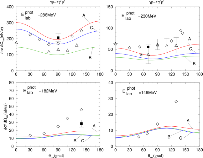
Figure 7: Variation of the differential cross section of the proton Compton scattering for the different propagator of the $\Delta^{+}$. The curve $A$,$B$ and $C$ relate to the expression of the $\Delta^{+}$ propagator (5.10),(5.12) and (5.16). The data are from ref. [25]

Fig. 7 shows the differential cross section for the elastic $\gamma p$ scattering reaction for the different energies of the incoming photon ($E_{lab}^{\gamma}=149,182,230,286MeV$) and with the different $\Delta$ isobar propagators. The sensitivity of these cross sections to the form of the $\Delta$ propagators increases in the $\Delta$ production region. Different curves on this Figure have the same qualitative behaviour. Therefore none of the three $\Delta$ propagators A(5.10), B(5.12) or C(5.16) seems to be more preferable according to the present comparison with the experimental datas [25].

Pion photoproduction reaction.

Our calculation of the $\gamma p\to{\pi^{o}}^{\prime}p^{\prime}$ reaction is based on the same set of diagrams as in ref. [16, 4], but our calculation is performed in the three dimensional, time-ordering form in the Coulomb gauge and with retardation effects included. These diagrams are depicted in the Fig. 8. As for proton Compton scattering, the one $N,\Delta$ exchange diagrams in the Fig.8a,b relates to the $s,u$ channel interaction terms. The $t$ channel is described by $\rho$ and $\omega$ meson exchange diagrams in the Fig.8c,d.

Figure 8: Pion photo-production on the proton. One particle $N,\Delta$ and $\rho,\omega$ exchange diagrams taken into account in the numerical calculation of the $\gamma p-{\pi^{o}}^{\prime}p^{\prime}$ reaction.

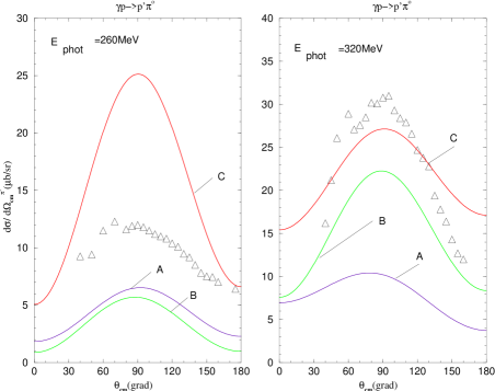
Figure 9: The differential cross sections for the pion photoproduction reaction for the $A$ (5.10), $B$ (5.12) and $C$ (5.16) $\Delta$ propagators. The experimental results indicated by triangles are from ref.[26].

Fig.9 shows the dependence of the differential cross section of the $\pi^{o}$ photoproduction $\gamma p\to{\pi^{o}}^{\prime}p^{\prime}$ on the $\Delta$ isobar propagators A,B and C for the two energies $(E_{lab}^{\gamma}=260,320MeV)$ of the incoming photon. As in the Compton scattering $\gamma p\to\gamma^{\prime}p^{\prime}$, the curves in the Fig.9 have qualitatively the same behavior as the experimental observables. But unlike to proton Compton scattering, the difference between the different propagators A,B,C is larger and this differences are more sensitive to the initial photon energy.

The $\gamma p\to\gamma^{\prime}{\pi^{o}}^{\prime}p^{\prime}$ reaction.

We now turn to the the $\gamma p\to\gamma^{\prime}{\pi^{o}}^{\prime}p^{\prime}$ reaction which we have calculated with the same vertex functions as the $\gamma p\to\gamma^{\prime}p^{\prime}$ and $\gamma p\to{\pi^{o}}^{\prime}p^{\prime}$ reactions (see Appendix A). For this calculation we have used the diagrams depicted in the Figure 10.

Figure 10: Diagrams for the $\gamma p\to\gamma^{\prime}{\pi^{o}}^{\prime}p^{\prime}$ reaction with one particle $N,\Delta$ and $\pi^{o}$, $\rho,\omega$ exchange which are taken into account in our numerical calculation. For the diagrams ${\bf b}$ and ${\bf e}$ contributions of the $\pi$-meson creation from the intermediate $N$ or $\Delta$ in the transitions $(N,N)$ $(N,\Delta)$ and $(\Delta,N)$ are included, but not the $\pi^{o}$ creation in the $(\Delta,\Delta)$ transition. In ref.[28] it is shown that this contribution is weak. In the $\rho,\omega$-meson exchange diagrams ${\bf g,h,i,j}$ only nucleon but not the $\Delta$ exchange is taken into account. In the one $\pi^{o}$-exchange diagrams ${\bf k,l}$ the dashed circle indicates the $\pi N$ scattering $t$-matrix.

For the one-$\Delta$ exchange diagrams we have calculated diagrams in the Fig. 10a,b,c,d,e,f, i.e. we have taken into account diagrams with $\Delta-\pi N$, $\Delta-\gamma N$, $\Delta-\gamma\Delta$ transitions and we have omitted diagrams with $\Delta-\pi\Delta$ vertex. In our calculation we have included diagrams with $\rho,\omega$ exchange (Fig.10g,h,i,j) which gives the important contributions in the $\gamma p\to{\pi^{o}}^{\prime}p^{\prime}$ reaction and also diagrams with one $\pi^{o}$ exchange (Fig.10k,l) which are important for the $\gamma p\to\gamma^{\prime}p^{\prime}$ reaction. The $\pi N$ scattering $t$-matrix in the Figs.10k,l is approximated by the $N,\Delta$-exchange $s,u$-channel terms. Due to the small $\pi^{o}$ decay coupling constant (see eq. (A.9) in Appendix A), contributions of the $\pi^{o}$ exchange diagrams ( Fig.10k,l) are small (less as $1\%$ in our calculation of the corresponding cross section).

The main goal of our calculation of the reaction $\gamma p\to\gamma^{\prime}{\pi^{o}}^{\prime}p^{\prime}$ is to estimate the contributions of background diagrams which are mixed with the diagram with the $\Delta-\Delta\gamma^{\prime}$ transition (Fig.10a). This diagram contains the interesting value of the $\Delta^{+}$ magnetic moment $\mu_{\Delta}$ (eq. (A.7) in Appendix A) and gives the most important contribution for the determination of the magnetic moment of the $\Delta^{+}$ resonance. An other diagram with a $\Delta-\Delta\gamma$ transition is depicted in Fig.10d. But the contribution of this diagram is not important for the cross sections. The complete number of the calculated diagrams is 38 (four diagrams of Fig.10a,b,c,d; $-2$ diagrams with the $\Delta-\pi\Delta$ transition in Fig.10b,e; $2\times 4=8$ diagrams in Fig.10g,h,i,j and two diagrams in Fig.10k,l with $s,u$-channel $N,\Delta$ exchange $\pi N$ interaction. $4\times 6-2+2\times 4+2\times 4=38$).

The first questions in estimating the background diagrams is: what is the contribution of the diagrams with $N-\gamma^{\prime}N$ transition which generates an infrared (bremsstrahlung with a $1/E_{\gamma^{\prime}}$ energy dependence) behaviour in the cross sections? In order to answer this question, let us consider Fig.11, where the cross section $d\sigma/dE_{\gamma^{\prime}}d\Omega^{\gamma^{\prime}}_{cm}$ with $E_{\gamma}^{lab}=348,398,449MeV$, $\theta_{cm}^{\gamma^{\prime}}=110grad;\phi_{cm}^{\gamma^{\prime}}=0$ and for the Breit-Wigner type propagator (model B, eq. (5.12)) are shown. The full curve includes the contributions of all diagrams in Fig.10, the long-dashed curve corresponds to the contribution of the single diagram with $\Delta-\gamma^{\prime}\Delta$ transition (Fig.10a with intermediate $\Delta^{\prime}s$) and long dashed curve includes the contributions of all diagrams without infrared $p-\gamma^{\prime}p^{\prime}$ transition. Thus from the Fig.11 we see that the contribution of the term with the interesting $\Delta-\gamma^{\prime}\Delta^{\prime}$ transition (Fig.10a) is comparable with the contributions of all other diagrams only at energies of the emitted $\gamma^{\prime}$ at around $80MeV$ ($E_{\gamma^{\prime}}^{cm}\simeq 80MeV$). The contribution of this diagram is further increased by increasing of the energy of the initial photon. The contribution of the diagram $\Delta\to\Delta^{\prime}\gamma^{\prime}$ in Fig.11, which is proportional to the magnetic moment of the $\Delta^{+}$ is most important for the following direction of the emitted photon $\theta_{cm}^{\gamma^{\prime}}=110grad;\ \phi_{cm}^{\gamma^{\prime}}=0$. Thus the most preferable kinematical region for the investigation of the role of the $\Delta-\gamma^{\prime}\Delta$ transition in the $\gamma p\to\gamma^{\prime}{\pi^{o}}^{\prime}p^{\prime}$ reaction is $E_{\gamma^{\prime}}^{cm}>80MeV$ and $\theta_{cm}^{\gamma^{\prime}}\sim 110grad;\ \phi_{cm}^{\gamma^{\prime}}\sim 0grad$.

Figure 11: The cross section $d\sigma/dE_{\gamma^{\prime}}d\Omega^{\gamma^{\prime}}_{cm}[nb/MeVsr]$ of the $\gamma p\to\gamma^{\prime}{\pi^{o}}^{\prime}p^{\prime}$ reaction with the $\Delta$ propagator of the Breit-Wigner shape (5.12) and for different energies of the incoming photon $|{\bf k}_{\gamma}|\equiv E_{\gamma}$. The dashed line corresponds to our calculation without $p-\gamma^{\prime}p^{\prime}$ or $p^{\prime}-\gamma^{\prime}p$. The long-dashed line is our result with only the diagram with the $\Delta-\gamma^{\prime}\Delta^{\prime}$ transition. The full curve includes the contributions of all diagrams in Fig.10.

In Fig.12 the same cross sections as in Fig.11 are displayed but with different $\mu_{\Delta}=2.79\mu_{N}$ and $\mu_{\Delta}=2\times 2.79\mu_{N}$ magnetic moments of the $\Delta^{+}$ resonance. The difference between corresponding curves by $E_{\gamma}^{lab}=348$ and $398MeV$ is quantitative and roughly no more than $10\%$. But for the $E_{\gamma}^{lab}=449MeV$ this difference is more significant.

Figure 12: The same cross section as in the Fig.11 but with a fixed energy of the emitted photon and variations of the photon emission angle. The dotted line by the $\theta_{[cm]}^{\gamma^{\prime}}=0\ grad$ corresponds to $\mu_{\Delta}=2.79\mu_{N}$ and solid line relates to $\mu_{\Delta}=2\times 2.79\mu_{N}$.

In Fig.13 and Fig.14 we show the cross sections $d\sigma/d{E^{\gamma^{\prime}}}_{cm}$ and $d\sigma/d{\Omega^{\gamma^{\prime}}}_{cm}$ for the different energies of the initial photon ($E_{\gamma}^{lab}=348$, $398$ and $449MeV$ corresponds to $s^{1/2}=1239$, $1277$ and $1318MeV$) and with the different $\Delta$ propagators from the model A,B,C of section 5. The difference between corresponding curves is large and most important for small . But the sensitivity of these curves on the different values of the $\Delta^{+}$ magnetic moment is small $<10\%$. The exception is in Fig.14 for the total energy $s^{1/2}=1239MeV$ corresponding to ${E^{\gamma}}_{lab}=348MeV$, where the $\Delta$ propagator of model C (5.16) was used for magnetic moments $\mu_{\Delta^{+}}=2.79$ and $2\times 2.79[nuclear\ magnetons]$.

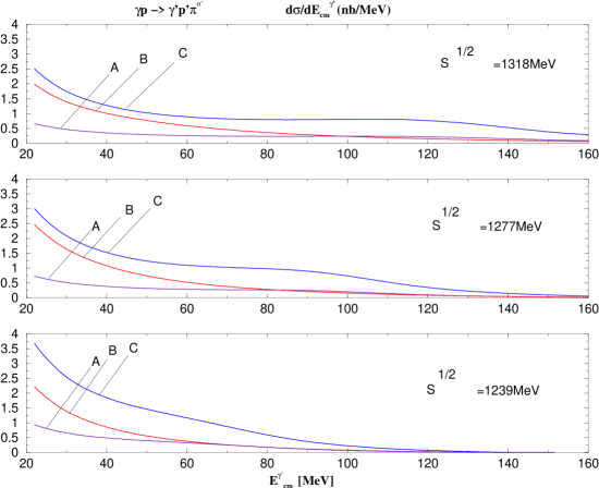
Figure 13: Cross section $d\sigma/d{E^{\gamma^{\prime}}}_{cm}[nb/MeV]$ as function of the energy of emitted photon $\gamma^{\prime}$ for the incident photon energies $E_{\gamma}=348,\ 398$ and $449$MeV for the different $\Delta$ propagators $A$ (eq.(5.10)), $B$ (eq.(5.12)) and $C$ (eq.(5.16)) For the magnetic moment $\mu_{\Delta^{+}}=2.79[nuclear\ magnetons]$ has been assumed.

The curves in Fig.13 and 14 qualitatively describe the experimental data which has been measured recently by the A2/TAPS collaboration at MAMI[5]. But the sensitivity of the calculated cross section $d\sigma/d{E^{\gamma^{\prime}}}_{cm}$ and $d\sigma/d{\Omega^{\gamma^{\prime}}}_{cm}$ on the magnitude of the $\Delta^{+}$ magnetic moment is even smaller as in the corresponding calculation in ref.[4]. This difference can be explained with the different gauge conditions, different number of included diagrams, with the missing retardation effects in ref.[4] etc. Only more complete calculations of the multichannel $\gamma p$ scattering equations with unitarity and a more consistent model of the $\Delta$ propagator, with rescattering effects in the nonresonant $\pi N$ interactions and antinucleon degrees of freedom can quantitative determine the interesting differential cross sections. Keeping in mind, that the cross sections of the $\gamma p\to\gamma^{\prime}{\pi^{o}}^{\prime}p^{\prime}$ reaction are much more sensitive to the form of the $\Delta$ particle propagator as to the magnitude of the $\Delta^{+}$ resonance, there appear the next question: is the present sensitivity of these differential cross sections enough for determination of the magnetic moment of the $\Delta^{+}$ resonance? Or in other words, exists a kinematical region where results of our calculation are qualitatively depending on $\mu_{\Delta^{+}}$? In order to find the kinematical region, where the the dependence on $\mu_{\Delta}$ is largest, we will consider the following cross sections:

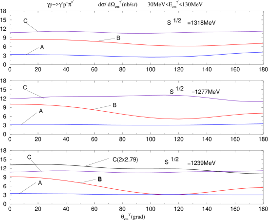
Figure 14: Angular distribution $d\sigma/d{\Omega^{\gamma^{\prime}}}_{cm}[nb/sr]$ of the final photon $\gamma^{\prime}$. The different curves represent the three different approaches for the $\Delta$ propagator and three different initial photon energies as in the previous Figure. For $s^{1/2}=1239MeV$ and $\Delta$ propagator of model $C$ (eq.(5.16)) the angular distribution of the emitted $\gamma^{\prime}$ is calculated for two magnetic moments $(2.79\ and\ 2\times 2.79)[nuclear\ magnetons]$ of the $\Delta^{+}$ resonance.

In Fig.15 we show the sensitivity of the angular distribution $d\sigma/d\Omega^{\gamma^{\prime}}_{cm}$ to the A (5.10), B (5.12) and C (5.16) models of $\Delta$ propagators and to the three different value of the $\Delta^{+}$ magnetic moment $\mu_{\Delta^{+}}=0,\ 3\mu_{N},\ 6\mu_{N}$. Calculations are performed for two values of the initial photon energy ${E^{\gamma}}_{lab}=400MeV$ and $450MeV$, where the energies of final photon are integrated over the following intervals: $80<{E^{\gamma^{\prime}}}_{cm}<150MeV$ and $100<{E^{\gamma^{\prime}}}_{cm}<150MeV$. For ${E^{\gamma}}_{lab}=400MeV$ the variation of $\mu_{\Delta^{+}}$ gives an essential difference of about $\sim 20\%$ for the model C of the $\Delta$ propagator. This difference decreases for ${E^{\gamma}}_{lab}=450MeV$. In this case the cross sections for the $\mu_{\Delta^{+}}=0$ and $3\mu_{N}$ practically coincides. This is different to the case with ${E^{\gamma}}_{lab}=400MeV$, where the curves with $\mu_{\Delta^{+}}=0$ and $6\mu_{N}$ are close to each other. But one obtains a different result for $\mu_{\Delta^{+}}=3\mu_{N}$. The values of the cross sections A and B are close to the experimental data [5], but these curves are less dependent on $\mu_{\Delta^{+}}$. In addition the behaviour of cross sections A are quantitatively different for the ${E^{\gamma}}_{lab}=400MeV$ and for the ${E^{\gamma}}_{lab}=450MeV$.

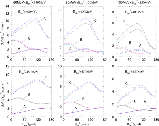
Figure 15: Variation of the angular distribution $d\sigma/d\Omega^{\gamma^{\prime}}_{cm}[nb/sr]$ of the final photon $\gamma^{\prime}$energies, for different energies of the initial photon $\gamma$, for different propagators of the $\Delta$ (A,B,C see text) and for different values of the magnetic moments of the $\Delta^{+}$. The dashed line corresponds to $\mu_{\Delta}=0$. The full curve for the values $\mu_{\Delta}=3\mu_{N}$ and dotted line relates to the $\mu_{\Delta}=6\mu_{N}$. The energies of the final photons ${E^{\gamma^{\prime}}}_{cm}$ are integrated over different intervals: $60<{E^{\gamma^{\prime}}}_{cm}<150MeV$, $80<{E^{\gamma^{\prime}}}_{cm}<150MeV$ and $100<{E^{\gamma^{\prime}}}_{cm}<150MeV$ for two initial photon energies: ${E^{\gamma}}_{lab}=400MeV$ and ${E^{\gamma}}_{lab}=450MeV$.

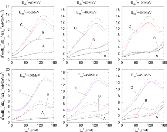
Figure 16: The angular distribution for the five-fold cross section $d^{5}\sigma/dE^{\gamma^{\prime}}_{cm}d\Omega^{\gamma^{\prime}}_{cm}d\Omega^{\pi^{\prime}}_{cm}[nb/GeVsr^{2}]$ for the following angles of the final photon and pion $\phi_{\gamma^{\prime}}=0^{o}$, ${\theta^{\pi^{\prime}}}_{lab}=15^{o}$ and $\phi_{\pi^{\prime}}=0^{o}$.

The sensitivity of the cross sections to different models of $\Delta$ propagators and to the $\Delta^{+}$ magnetic moments $\mu_{\Delta^{+}}=0,3\mu_{N},6\mu_{N}$ is examined also in the Figure 16, where the five-fold cross sections $d^{5}\sigma/d^{3}{\bf k^{\prime}}^{\gamma^{\prime}}_{cm}d\Omega^{\pi^{\prime}}_{cm}$ with fixed values of the scattering angles $\phi_{\gamma^{\prime}},{\theta^{\pi^{\prime}}}_{lab},\phi_{\pi^{\prime}}$ and the emitted photon energy are shown. Unlike to the previous Figure, here the difference between the curves with different $\mu_{N}$ is more visible. Most promising is here the quantitative difference between differential cross sections for the model B with ${E^{\gamma}}_{lab}=450MeV$ and $\mu_{\Delta^{+}}=0$, $\mu_{\Delta^{+}}=3\mu_{N}$ and $\mu_{\Delta^{+}}=6\mu_{N}$. This difference is not only very large, but also quantitatively different as for the incident photon energy ${E^{\gamma}}_{lab}=400MeV$.

Thus we see that in special kinematical regions the sensitivity of differential cross sections of the $\gamma p\to\gamma^{\prime}{\pi^{o}}^{\prime}p^{\prime}$ reaction to the magnitude $\mu_{\Delta^{+}}$ can be large and this difference can have a qualitative nature. The corresponding kinematical region is different for the different $\Delta$ propagators. But the region with the ${E^{\gamma}}_{lab}>400MeV,{E^{\gamma^{\prime}}}_{lab}>80MeV\ and\ {\theta^{\gamma^{\prime}}}_{cm}\simeq 110^{o}$ is most preferable for the determination of the $\Delta^{+}$ magnetic moment $\mu_{\Delta^{+}}$.

7. Conclusion

The present paper is devoted to the unified field-theoretical formulation of the multichannel $\gamma p\to\gamma^{\prime}p^{\prime}$, $\gamma p\to{\pi^{o}}^{\prime}p^{\prime}$ and $\gamma p\to\gamma^{\prime}{\pi^{o}}^{\prime}p^{\prime}$ reactions and their calculation in the framework of the one-particle exchange model. The field theoretical formulation was carried out in the framework of the “old fashioned perturbation theory” or spectral decomposition method over the asymptotical (Fock space) states. The present relativistic formulation has the following attractive features:

• 1. Unlike other relativistic approaches [4], our resulting amplitudes of the $\gamma p$ multichannel reactions takes into account all retardation effects. The formulation is from the beginning three dimensional and therefore it is free from the ambiguities which are appearing by the three dimensional reduction of the four dimensional Bethe-Salpeter equations [11, 12, 15]. The use of the three-dimensional relativistic equation derived in the framework of the old perturbation theory is convenient, because in this formulation the scattering amplitudes have a minimal off-shellness and the off-shell contributions of external and internal particles can be distinguished in the potential. Moreover, in the three-dimensional relativistic approach considered here, the effective potential (or exchange currents) are constructed from one-variable vertex functions, i.e., vertex functions with two on-mass shell particles. In all other field-theoretical approaches the effective potentials (or exchange currents) are defined by vertices depending on two or three variables. Therefore in these formulations severe approximations are necessary: there nucleon and $\Delta$ off-mass shellness is usually neglected.

• 2. The complete set of the time-ordered diagrams of the $\gamma p\to\gamma^{\prime}\pi^{\prime}N^{\prime}$ reactions with off mass shell $\gamma,\gamma^{\prime}$ and $\pi^{\prime}$ is presented and analyzed. The general structure of the corresponding diagrams and scattering amplitudes does not depend on the choice of the model of an effective Lagrangian. The field-theoretical equations considered above are exactly connected with all other field-theoretical equations i. e. we can derive the Bethe-Salpeter equation in the framework of the $S$-matrix reduction technique. Therefore, all results obtained in the framework of this time-ordered, three-dimensional equations remain valid in other field-theoretical approaches as well.

• 3. It was shown that in the suggested equations for amplitudes of the $\gamma N\to\gamma^{\prime}{\pi^{o}}^{\prime}N^{\prime}$ reaction with Coulomb gauge the current conservation condition is automatically satisfied if the requirement of the current conservation for the photon-hadron vertex functions is fulfilled. Therefore, unlike in refs. [16, 7, 17, 18, 19, 20, 4], it is not necessary to restrict the number of the calculated diagrams, or to combine some diagrams in the tree approximation, or to make additional assumptions about the $\Delta$ propagator in order to ensure the current conservation.

• 4. The separable model of the $\pi N$ interaction is generalized for the case of the construction of the spin $3/2$ particle propagator of the $\Delta$-resonance. This procedure allows us to obtain the $\pi N\to\Delta$ form-factor and $\Delta$ propagator directly from the $\pi N$ $P_{33}$ phase-shifts and afterwards use these spin $3/2$ particle propagator in the microscopic calculations.

The numerical calculations of the differential cross section of the $\gamma p\to\gamma^{\prime}N^{\prime}$, $\gamma p-\pi^{\prime}N^{\prime}$ and $\gamma p\to\gamma^{\prime}{\pi^{o}}^{\prime}p^{\prime}$ reactions are performed in the framework of the one-particle $N$,$\Delta$ and $\pi$,$\rho$,$\omega$ exchange model with two different separable models of the $\Delta$ propagator and with the Breit-Wigner propagator. The main numerical result is that the description of the multichannel $\gamma p$ scattering reactions in the $\Delta$ resonance region is strongly dependent on the choice of the form of the $\Delta$-propagator. Moreover, the difference between cross sections of the $\gamma p\to\gamma^{\prime}{\pi^{o}}^{\prime}p^{\prime}$ reaction with different $\Delta$ propagators in the special kinematical region is larger than for the $\gamma p\to\gamma^{\prime}p^{\prime}$ and $\gamma p\to{\pi^{o}}^{\prime}p^{\prime}$ reactions. This result makes it necessary to examine the theoretical model of the $\Delta$ resonance and vertex functions based on the $\gamma p\to\gamma^{\prime}{\pi}^{\prime}N^{\prime}$ reactions in addition to the photon Compton scattering and pion photoproduction reactions.

The sensitivity of the reaction $\gamma p\to\gamma^{\prime}{\pi^{o}}^{\prime}p^{\prime}$ to the different values of the $\Delta^{+}$ magnetic moment $\mu_{\Delta^{+}}$ is examined. This sensitivity is less than $10\%$ for most differential cross sections, measured in ref.[5]. However it was demonstrated that for every $\Delta$ propagator some special kinematical region exists, where differences between calculated cross sections with different $\mu_{\Delta^{+}}$ are qualitative and yild even an effect of more than $25\%$. This findings make it possible to extract in future with more improved calculations the magnitude of the $\mu_{\Delta^{+}}$ from the experimental data of $\gamma p\to\gamma^{\prime}N^{\prime}$, $\gamma p-\pi^{\prime}N^{\prime}$ reaction.

Acknowledgment

Authors thank D. Drechsel, M.I. Krivoruchenko and M. Vanderhaeghen for discussions. We would like to express our gratitude to M. Kotulla and V. Metag for the current interest to this work and for useful remarks.

Appendix A. Vertex functions.

In the considered formulation nucleon and $\Delta$ isobar are defined on mass shell i.e. $N$ and $\Delta$ are included only in the bracket vector as ordinary one-particle states. Therefore the three particle vertex functions with nucleons and $\Delta$ isobars are depending only on the four-momentum transfer $t$. In our calculation we have used the following vertex functions:

The $\gamma N-N$ vertex function in the Coulomb gauge is given in eq. (3.2) and (3.4)[8]. The exact form of the formfactors $F_{1,2}(t)$ is considered, for example in ref. [29]. In our calculation for the photon-proton vertex function we have taken $F_{1}(t)=F_{2}(t)\equiv f(t)=(1-t/a^{2})^{-2};\ \ \ a=0.249fm;\ \ \ \mu_{N}=1.79.$

$\pi N-N$ vertex function is taken from the dispersion relation analysis [10]

$$<{\bf p^{\prime}}_{N}|j_{\alpha}(0)|{\bf p}_{N}>=iG(t){\overline{u}}({\bf p})\gamma_{5}\tau_{\alpha}u({\bf p});\ \ \ G(t)=g_{\pi N}\Bigl{(}1+{{t(t-4m_{N}^{2})}\over{4m_{N}^{2}m_{o}^{2}}}\Bigr{)}^{-1}$$

where $m_{o}=8.6m_{\pi};\ \ \ g_{\pi N}=12.78$.

$\gamma N-\Delta$ vertex function of Jones-Scadron [21] . In this treatment $p_{\Delta}$ is the four vector the spin $3/2$ particles with the real mass $m_{\Delta}$ i.e. $p_{\Delta}=(\sqrt{m_{\Delta}^{2}+{\bf p}^{2}},{\bf p})$ and

$$<{\bf p^{\prime}}_{N}|J^{\mu}(0)|{\bf p}_{\Delta}>\equiv\biggl{\{}<{\bf p^{\prime}}_{N}|J^{\mu}(0)\biggr{\}}_{\pi N\ irreducable}|\Psi_{{\bf p}_{\Delta}}>=$$

$${\overline{u}}({\bf p^{\prime}}_{N})\biggl{[}F_{M}(t)\Gamma_{M}^{\mu\nu}(t)+F_{E}(t)\Gamma_{E}^{\mu\nu}(t)+F_{C}(t)\Gamma_{C}^{\mu\nu}(t)\biggr{]}u_{\nu}({\bf p}_{\Delta})$$

where $t=({p^{\prime}}_{N}-p_{\Delta})^{2}$ and magnetic $\Gamma_{M}^{\mu\beta}(t)$, electric $\Gamma_{E}^{\mu\beta}(t)$ and charged $\Gamma_{C}^{\mu\beta}(t)$ Lorentz-invariant combination are defined as

$$\Gamma_{M}^{\mu\nu}(t)=-{3{(m_{N}+m_{\Delta})}\over{2m_{N}\Bigl{(}(m_{N}+m_{\Delta})^{2}-t\Bigr{)}}}\epsilon^{\mu\nu\alpha\sigma}(p^{\prime}_{N}+p_{\Delta})_{\alpha}(p_{\Delta}-p^{\prime}_{N})_{\sigma}$$

$$\Gamma_{E}^{\mu\nu}(t)=-\Gamma_{M}^{\mu\nu}(t)$$

$$-\gamma_{5}\ {3i{(m_{N}+m_{\Delta})}\over{m_{N}\Bigl{(}(m_{N}+m_{\Delta})^{2}-t\Bigr{)}\Bigl{(}(m_{N}-m_{\Delta})^{2}-t\Bigr{)}}}\epsilon^{\mu\lambda\alpha\beta}(p^{\prime}_{N}+p_{\Delta})_{\alpha}(p_{\Delta}-p^{\prime}_{N})_{\beta}\epsilon^{\nu\gamma\delta}_{\lambda}{p_{\Delta}}_{\gamma}(p_{\Delta}-p^{\prime}_{N})_{\delta}$$

$$\Gamma_{C}^{\mu\nu}(t)=-\gamma_{5}\ {3i{(m_{N}+m_{\Delta})(p_{\Delta}-p^{\prime}_{N})^{\mu}\Bigl{[}t(p^{\prime}_{N}+p_{\Delta})^{\nu}-(p_{\Delta}-p^{\prime}_{N})^{\nu}(m_{\Delta}^{2}-m_{N}^{2})\Bigr{]}}\over{2m_{N}\Bigl{(}(m_{N}+m_{\Delta})^{2}-t\Bigr{)}\Bigl{(}(m_{N}-m_{\Delta})^{2}-t\Bigr{)}}}.$$

Charge formfactor $\Gamma_{C}^{\mu\nu}(t)$ contributes in the our calculation with the retardation. But in the tree approximation, where the four vector $q^{\mu}=(p_{\Delta}-p^{\prime}_{N})^{\mu}$ is replaced with the real photon four momentum $q^{2}=0$, contributions of $\Gamma_{C}^{\mu\nu}(t)$ disappears.

For the electric, magnetic and charge formfactors we take the same cut-off function $f(t)$ as for the $\gamma$-proton vertex function

$$F_{M}(t)=F_{M}(0)f(t);\ \ \ F_{E}(t)=F_{E}(0)f(t);\ \ \ F_{C}(t)=F_{C}(0)f(t)$$

where $F_{M}(0)=3.2$ [30], $F_{E}(0)=0.025F_{M}(0)$ [32] $F_{E}(0)=(m_{\Delta}-m_{N})/2m_{\Delta}F_{C}(0)$ [21]. For our numerical calculation most sufficient is the magnetic part of (A.2). The recent overview of the unified $N^{*}-N\gamma$ vertex functions is given in [31].

The $\pi N-\Delta$ vertex function are defined in section 5. Thus in the model A $\pi N-\Delta$ vertex function is $g({\bf p})$ (5.11), in model B it coincides with the coupling constant (5.13) and in model C $\pi N-\Delta$ vertex function is $h({\bf p})$ (5.15).

The $\gamma\Delta^{\prime}-\Delta$ vertex functions are the same as in our previous paper [2]. In this case $Q=P^{\prime}_{\Delta}-P_{\Delta}$ and $R=P^{\prime}_{\Delta}+P_{\Delta}$ and $\gamma\Delta^{\prime}-\Delta$ vertex function is

$$<{\bf P^{\prime}}_{\Delta}|J_{\mu}(0)|{\bf P}_{\Delta}>={\overline{u}}^{\sigma}({\bf P^{\prime}}_{\Delta})V_{\sigma\mu\rho}({\bf P^{\prime}}_{\Delta},{\bf P}_{\Delta})u^{\rho}({\bf P}_{\Delta})$$

where

$$V_{\sigma\mu\rho}({\bf P^{\prime}}_{\Delta},{\bf P}_{\Delta})=g_{\rho\sigma}\Bigl{[}F_{1}(Q^{2})\gamma_{\mu}+{{F_{2}(Q^{2})}\over{2M_{\Delta}}}R_{\mu}\Bigr{]}+Q_{\sigma}Q_{\rho}\Bigl{[}{{F_{3}(Q^{2})}\over{M_{\Delta}^{2}}}\gamma_{\mu}+{{F_{4}(Q^{2})}\over{2M_{\Delta}^{3}}}R_{\mu}\Bigr{]}.$$

The form factors $F_{i}(Q^{2})$ are simply connected with the charge monopole $G_{C0}(Q^{2})$, the magnetic dipole $G_{M1}(Q^{2})$, the electric quadrupole $G_{E2}(Q^{2})$ and the magnetic octupole $G_{M3}(Q^{2})$ form factors of the $\Delta^{+}$ resonance. In the low energy region we can neglect the terms $\sim Q^{2}/4M_{\Delta}^{2}$, and we keep only terms $\sim 1/M_{\Delta}$. Then the previous formula can be rewritten in a similar form as the $\gamma$-proton vertex function:

$$V_{\sigma\mu\rho}({\bf P^{\prime}}_{\Delta},{\bf P}_{\Delta})=g_{\rho\sigma}G_{C0}(Q^{2}){{R_{\mu}}\over{2M_{\Delta}}}+ig_{\rho\sigma}{{G_{M1}(Q^{2})}\over{2M_{\Delta}}}\sigma_{\mu\beta}Q^{\beta}$$

In our case of soft photon emission we have approximated the form factors in (A.7) with their pseudo-threshold values $G_{C0}(Q^{2})\to G_{C0}(t_{ptr}=1$ and $G_{M1}(Q^{2})\to G_{M1}(t_{ptr})=\mu_{\Delta^{+}}$, where $t_{ptr}=(m_{\Delta}-m_{N})^{2}$, $\mu_{\Delta^{+}}$ denotes the magnetic moment of the $\Delta^{+}$ resonance and it is simply connected with the $k_{\Delta^{+}}$ anomalous magnetic moment of $\Delta^{+}$ $\mu_{\Delta^{+}}=(1+k_{\Delta^{+}})/2m_{\Delta}$.

The $V\equiv\rho,\omega$ meson-nucleon vertex functions in eq. (2.11) have the form

$$<{\bf p^{\prime}}_{N}|j^{V}_{\mu}(0)|{\bf p}_{N}>={\overline{u}}({\bf p^{\prime}}_{N})\Biggl{(}\gamma_{\mu}F^{V}_{1}(t)+i{{k_{V}}\over{2m_{N}}}\sigma_{\mu\nu}(p_{N}^{\prime}-p_{N})^{\nu}F^{V}_{2}(t)\Biggr{)}u({\bf p}_{N})$$

where $k_{\omega}=0;\ \ k_{\rho}=3.7$. Form factors $F^{V}_{1}(t)$ are replaced with their threshold values $F^{V}_{1}(t)\Longrightarrow g_{VNN}$ and $g_{\omega NN}=3\times g_{\rho NN}=15$ [33]. And for the $\rho(\omega)$ decay constant we have taken the value $g_{\omega\gamma\pi}=3\times g_{\rho\gamma\pi}=0.374$ [16, 34].

The $\pi^{o}$ decay vertex function in the Figure 10k,l is taken in the standard form on the tree approximation [27, 19]

$$\Gamma_{\gamma^{\prime}-\pi^{o}\gamma}^{\mu\nu}\sim\int d^{4}x<0|T\Bigl{(}j^{\mu}(x)j^{\nu}(0)\Bigr{)}|{\bf p_{\pi}}={\bf k}_{\gamma}-{\bf k}_{\gamma^{\prime}}>e^{ik_{\gamma^{\prime}}x}\approx-i{0.035\over{m_{\pi}}}\epsilon^{\mu\nu\alpha\beta}{k_{\gamma}}_{\alpha}{k_{\gamma^{\prime}}}_{\beta}.$$

References

[1] L. A. Kondratyuk and L. A. Ponomarev, Sov. J. Nucl. Phys.
7(1968) 82.
[2] A. I. Machavariani, Amand Faessler, and
A. J. Buchmann, Nucl. Phys. A646 (1999) 231; Nucl. Phys.
A686 (2001) 601.
[3] D. Drechsel, M. Vanderhaeghen, M.M.Giannini
and E. Santopinto, Phys. Lett. B 484 (2000)236.
[4] D. Drechsel and M. Vanderhaeghen, Phys.Rev.
C64 (2001) 065202.
[5] M. Kotulla and V. Metag, private communications;
M. Kotulla, Proc. of the Workshop on Phys. of Exited Nucleons (Nstar
2001), Mainz,Germany, 2001 (to be published);
M. Kotulla, Dissertation, Physikalisches Institute,
Universitaet Giessen 2001.
[6] R. Beck, B. Nefkens et al, Letter of Intent,
MAMI (2001).
[7] J.V. Boss and J.H. Koch Nucl. Phys.
A563 (1993) 539.
[8] J. D. Bjorken and S.D.Drell,
Relativistic Quantum Fields. (New York, McGraw-Hill) 1965.
[9] C. Itzykson and C. Zuber.
Quantum Field theory. (New York, McGraw-Hill) 1980.
[10] M. K. Banerjee and J. B. Cammarata, Phys. Rev. C17 (1978) 1125.
[11] A. I. Machavariani, Fiz. Elem. Chastits At Yadra 24 (1993)
731.
[12] A. I. Machavariani, Few-Body Phys. 14 (1993) 59.
[13] V. De Alfaro, S. Fubini, G. Furlan and C. Rosseti,
Currents in Hadron Physics (North-Holland, Amsterdam) 1973.
[14] A. I. Machavariani and
A. G. Rusetsky, Nucl. Phys. A515 (1990) 621.
[15] A. I. Machavariani, A. J. Buchmann, Amand Faessler, and
G. A. Emelyanenko, Ann. of. Phys. 253 (1997) 149.
[16] S. Nozawa, B. Blankleider and T.-S.H. Lee. Nucl. Phys.
A513 (1990) 459.
[17] H. Ohta, Phys.Rev. C40 (1989) 1335.
[18] H. Haberzettl, Phys.Rev. C62 (2000) 03465;
H. Haberzettl, C. Bennnold and T. Mart, Acta Phys. Polonica.
B31 (2000) 2387.
[19] V. Pascalustsa and O. Sholten, Nucl.
Phys.A 591 (1995) 658.
[20] M. El Amiri, G. Lopez Castro and J. Pestiau, Nucl. Phys.
A543 (1992) 673; G. Lopez Castro and A. Mariano, nucl-th/0010045.
[21] H. F. Jones and M. D. Scadron, Ann. Phys.
81 (1973) 1.
[22] L. Heller, S. Kumano, J. C. Martinez, and E. J. Moniz,
Phys. Rev. C35 (1987) 718.
[23] G. E. Groom at al. (PDG), Eur. J. Phys.
C15 (2000) 1.
[24] H. Garcilazo and T. Mizutani, systems;
(World Scientific, Singapore) 1990.
[25] E. L. Hallin at all, Phys.Rev. C48 (1993) 1497.
[26] H. Genzel at al, Z.PHYS.279 (1976) 399.
[27] T. P. Cheng and Ling-Fong Li,
Gauge theory of elementary particle physics. (Oxford, Clarendon Press) 1984.
[28] W. E. Fischer and P. Minkowski, Nucl. Phys.
B36 (1972) 519.
[29] M.. M. Giannini, Rep. Prog. Phys.54 (1991) 483.
[30] D. Drechsel, O.Hansen,S.Kamalov and
L. Tiator, Nucl.Phys. A645 (1999) 145.
[31]
M. I. Krivoruchenko, B. V. Martemyanov, A. Faessler and C. Fuchs,
arXiv:nucl-th/0110066, Ann. Phys. (N.Y.), in press.
[32] R. Beck et al, Phys.Rev.
C61 (2000) 035204.
[33] M. Guidal, J. M. Laget and M. Vanderhaeghen, Nucl. Phys.
A627 (1997) 645.
[34] Amand Faessler, C. Fuchs and M.I. Krivoruchenko, Phys. Rev.
C61 (2000) 035206.