Comparison of Form Factors Calculated with Different Expressions for the Boost Transformation

Abstract

The effect of different boost expressions is considered for the calculation of the ground-state form factor of a two-body system made of scalar particles interacting via the exchange of a scalar boson. The aim is to provide an uncertainty range on methods employed in implementing these effects as well as an insight on their relevance when an “exact” calculation is possible. Using a wave function corresponding to a mass operator that has the appropriate properties to construct the generators of the Poincaré algebra in the framework of relativistic quantum mechanics, form factors are calculated using the boost transformations pertinent to the instant, front and point forms of this approach. Moderately and strongly bound systems are considered with masses of the exchanged boson taken as zero, 0.15 times the constituent mass $m$, and infinity. In the first and last cases, a comparison with “exact” calculations is made (Wick-Cutkosky model and Feynman triangle diagram). Results with a Galilean boost are also given. Momentum transfers up to $Q^{2}=100\,m^{2}$ are considered. Emphasis is put on the contribution of the single-particle current, as usually done. It is found that the present point-form calculations of form factors strongly deviate from all the other ones, requiring large contributions from two-body currents. Different implementations of the point-form approach, where the role of these two-body currents would be less important, are sketched.

, ,

1 Introduction

Implementing relativity in the description of form factors of few-body systems is an important task nowadays. Motivated for some part by experiments performed at high $Q^{2}$ at different facilities, especially JLab, this ingredient is required for correctly analyzing the measurements. Many approaches have been proposed, ranging from field-theory based to relativistic-quantum mechanics ones [1, 2, 3, 4, 5, 6, 7, 8, 9, 10], implying sometimes seemingly founded approximations. A full realistic calculation is difficult and since the calculation of the deuteron form factors by Tjon and Zuilhof [1], there are not so many calculations that have reached the same level of correctness and, simultaneously, of complexity. Full calculations can also be performed in other cases [11, 12], employing solutions of the Bethe-Salpeter equation [13] with a zero-mass boson (Wick-Cutkosky model [14, 15]) or an infinite one (Feynman triangle diagram). They are somewhat academic but turn out to be quite useful as a testing ground of the approximate treatment of relativity in many studies.

There are currently many recipes aiming to implement relativity in the description of some system with a reduced amount of effort. They imply for instance minimal relativity factors, $\sqrt{m/e}$, or relativistic energies in place of non-relativistic ones. When considering elastic form factors, that are of main interest here, one also has to deal with boosting appropriately the final state with respect to the initial one. Here too, one has looked for simple recipes. In the case of spin-less particles, the first effect one thinks of is the Lorentz-contraction. To account for it, it was proposed to make the following replacement in the non-relativistic calculation [5]

$$F^{NR}(Q^{2})\rightarrow F^{Rel}(Q^{2})=F^{NR}(Q^{2}/[1+Q^{2}/(4M^{2})]),$$ (1)

where M is the total mass of the system under consideration.

This relation, that is still being used [16, 17], can be recovered somewhat easily (it is obtained by a simple change of variable). Perhaps for this reason, it was believed to represent a realistic way to implement an important feature of relativity (see some discussion in Ref. [6]). However, it was realized later on that this prescription leads to constant form factors at high $Q^{2}$, in disagreement with what is expected from the consideration of the Born amplitude. This one underlies predictions of power law behavior of form factors at large $Q^{2}$ ($Q^{-2}$ and $Q^{-4}$ for the pion and nucleon form factors in QCD, respectively [18, 19], or $Q^{-4}$ for the ground state of a system of scalar particles exchanging a scalar boson, as considered in this work [20]). On the other hand, Glöckle and Hamme [21] (see also [22]) analyzed solutions obtained from some Hamiltonian for a similar system. They found support for the Lorentz contraction but could not conclude whether the deviations were due to the approximate nature of their Hamiltonian.

Quite recently, another way to implement relativity in the calculation of form factors was proposed by Klink [10]. Supposed to be based on the point-form approach, it essentially relies on kinematical boost transformations. It has been applied for calculating form factors of the deuteron [23], the nucleon [24], a two-body system composed of scalar particles exchanging a zero-mass boson [11] and a system corresponding to a zero-range interaction [12]. In the first case, there is no significant improvement with respect to a non-relativistic calculation. In the second case, the agreement is at first sight spectacular, especially at the lowest $Q^{2}$ range considered by the authors. However, one can guess a tendency to an increasing under-prediction of the measurements in the highest range. In the third and fourth cases, there is no experiment but comparison is possible with what can be considered as an “exact” calculation as far as relativity is concerned. Corrections originating from the field-theory character of the underlying model, such as constituent form factors [25], cancel out in the comparison while they should be accounted for in the nucleon case mentioned above. In the last two cases, an important discrepancy shows up, especially in the limit of a zero-mass system or at large $Q^{2}$, which a relativistic approach should deal with. Two features emerge from these form factors when compared to “exact” calculations (as well as non-relativistic ones): point-form results evidence an increased charge radius and a rapid fall-off, faster than expected from the Born-amplitude.

In the present paper, we want to see in particular whether the peculiar features evidenced by recent calculations of form factors are specific to the point-form approach or characterize also other forms of relativistic quantum mechanics, such as the instant- and front-form. In this order, one can start from some mass operator, which enters in the construction of the generators of the Poincaré group [26, 27]. However, this does not indicate the connection between the dynamical variables entering this construction and the experimentally physical quantities [28, 29]. To establish this connection, a physical model has to be considered, while the underlying field-theory could provide an “exact”calculation of form factors, somewhat playing the role of a measurement. Thus, the interaction entering the mass operator should fulfill two different constraints. Besides those required to construct the generators of the Poincaré group, we demand that the interaction allows one to recover the field-theory one in the small coupling limit. This is the least that we can ask.

Steps of the above program can be found in the literature [26, 27] (see also for instance refs. [4, 30] in a slightly different context). For our purpose, we give some of them here, both for comprehensiveness and definiteness. As we want to know how an approach different from the point-form one does in comparison to an “exact” calculation, we will specialize in this work on the instant-form approach. While doing so, we give a particular attention to the change of variable which allows one to express the momenta of two particles, let’s say $\vec{p}_{1}$ and $\vec{p}_{2}$ for a two-body system, in terms of the total momentum, $\vec{P}$, and an internal variable, $\vec{k}$, which enters the mass operator. This relation, represented by a unitary transformation [28], is nothing but the one introduced by Bakamjian and Thomas [26]. It is essential for determining how a wave function obtained from some mass operator transforms when the system under consideration is boosted. The condition that the mass spectrum be independent of the momentum of the system is found to provide the standard constraints on the mass operator, from which the Bakamjian-Thomas construction of the generators of the Poincaré group immediately follows [26]. The mass operator so obtained can then be used for the front- or point-form approaches [27].

When available, we will give results of what can be considered an “exact” calculation (Wick-Cutkosky model, Feynman triangle diagram), the corresponding physics being supposed to be accounted for by the different approaches listed above. Due to the difficulty to fully account for this physics in the finite-mass boson case (the bound-state spectrum is not reproduced by the interaction model used to calculate the wave function employed in our study, and current conservation is not necessarily fulfilled), we will also present results obtained with a tentatively improved interaction. The comparison of the results will allow one to get some insight into the uncertainty due to the approximate description of the interaction. This aspect is in any case difficult to assess in quantum mechanics approaches which have to account effectively, in one way or another, for the field-theory character of the original model.

Concerns have been expressed about comparing approaches as different as field-theory and relativistic quantum mechanics, which correspond to problems with an indefinite and a fixed number of particles. We believe that this is what should be done if one wants to check the reliability of some relativistic quantum mechanics approach. When predictions of these approaches are compared to a measurement, they imply the underlying physics, QED, some meson theory or QCD. In all cases, this physics is field-theory based. We could also notice that comparisons similar to the present one have started long ago. Coester and Ostebee, for instance, noticed some agreement of their instant-form calculation for the deuteron form factor at low $Q^{2}$ [28] with a field-theory one by Gross [31]. Finally, we stress that the two approaches we are using are developed independently. There is no attempt to make some reduction of the Bethe-Salpeter equation, which is sometimes done. As noticed for instance by Lev (see introduction of ref. [32]), the description of a bound system in relativistic quantum mechanics represents an approximation to the one based on the Bethe-Salpeter equation but it offers the advantage that it preserves the covariance while the above reduction generally does not.

When comparing form factors calculated from different relativistic quantum mechanics approaches, we have in mind that, ultimately, they should coincide, in agreement with the idea that these approaches are equivalent, up to a unitary transformation [33]. The first step concerns the mass operator, already mentioned, whose solutions can be used in any scheme, only with different transformation properties when going from the variables, $\vec{p}_{1},\;\vec{p}_{2}$, to $\vec{P},\;\vec{k}$. The second step concerns the current which consists of a one-body part and, for a two-body system, a two-body one, which is interaction dependent. The contribution of this second part, when added to the former, should ensure the expected equivalence of the various relativistic quantum mechanics approaches. In this work, we will concentrate on the contribution of the single-particle current, most often retained in usual calculations of form factors. As significant differences appear at this level, making it difficult to realize the above unitary equivalence, we will give a particular attention to everything that can cast light on how these differences occur and manifest themselves.

Concerning the observables, we will consider charge and scalar form factors stemming from the coupling to Lorentz-vector and Lorentz-scalar probes, respectively. We are still interested in the ground state of a system composed of scalar particles interacting via the exchange of a scalar boson. Results, obtained for instant- but also front-, and point-form approaches, will be compared to what could be considered as an “exact” calculation. As it is a current practice to compare relativistic calculations to non-relativistic ones, we also include in our study results obtained by applying a Galilean boost. The corresponding wave functions are obtained from an effective, theoretically-motivated interaction which does well for the spectrum [34] and allows for a conserved current. The comparison of the different results for charge and scalar form factors will also evidence other features that are not related to the boost itself but are more or less related to standard exchange currents. These two-body currents, which are required, among other things, to fulfill covariance, will be evoked at many places in the paper but will not be the object of a systematic study. Some insight on their contribution will be obtained by looking at the form factors calculated in a frame different from the Breit one.

As already mentioned, comparison of form factors obtained in the instant form of relativistic quantum mechanics, on which some emphasis is put here, and those obtained in a field-theory framework have already been done in the past [28]. The system under consideration in the present work will not be as realistic as the one looked at in this earlier work. Instead, we consider situations where relativity is expected to play an essential role such as large momentum transfers or strongly bound systems, partly in relation with Lorentz-contraction effects. Accordingly, we do not make any $1/M^{2}$ approximation in dealing with the boost transformation.

The plan of the paper is as follows. In the second section, we concentrate on the interaction and its reduction to an invariant mass operator. This interaction allows one to establish some relation with field-theory in the weak coupling limit and is used for the determination of wave functions required for the calculation of form factors. This is done within the instant-form approach while the relation to the work by Bakamjian and Thomas is emphasized. The third section is devoted to the expression of the form factors we are calculating in different forms of relativistic quantum mechanics. Results up to $Q^{2}=100\,m^{2}$ are presented in the fourth section. They concern the scalar and charge form factors of the ground state of the system under consideration. Three masses of the exchanged boson, $\mu=0$ (Wick-Cutkosky model), $\mu=0.15\,m$ and $\mu=\infty$ are considered, as well as two masses for the system, $M\simeq 1.6\,m$, which implies a moderately bound system, and $M=0.1\,m$, which is an extreme case that a relativistic approach should in principle be able to deal with. The fifth section contains a discussion and the conclusion.

2 Choice of the two-body interaction

The starting point to calculate form factors supposes to determine wave functions from some equation together with some interaction. Quite generally, the corresponding mass spectrum depends on the momentum of the system under consideration and, therefore, is not covariant. Using a Hamiltonian formalism with a one-boson exchange interaction, the dependence was studied in refs. [21, 22], in relation with Lorentz-contraction effects. Amazingly, the violation of covariance was found rather small, due probably to the choice of appropriate ingredients (relativistic energies, single-particle normalization factors $\sqrt{m/e}$, etc). This lack of covariance can be ascribed to an incomplete description of the interaction. It can be remedied, but this assumes to determine the corrections to the interaction order by order.

In the present work, we will proceed in a slightly different manner, where the above covariance problem is easily solved, although indirectly. Not surprisingly, one finds a close relation to the work by Bakamjian and Thomas [26] developed within the instant-form of relativistic quantum mechanics. There, the covariance is verified provided that the interaction fulfills some constraints that will be recovered. Once this interaction is obtained, the construction of the generators of the Poincaré group is straightforward. As this construction has been given in many places, it is not repeated here. For our instant-form calculations of form factors, the main point concerns the transformation properties of the wave function from one frame to another one. These ones are accounted for automatically by directly considering the solutions of the appropriate equation in terms of the physical variables, rather than the variables most often introduced to construct the generators of the Poincaré group and, especially, the mass operator. However, the consideration of this latter one may be useful for calculations of form factors in the front-form or point-form approaches [27]. How to employ the solutions of the mass operator with this aim has been described in the literature [7, 8, 10].

2.1 Getting an invariant mass operator

Our starting point is an equation with ingredients purposely chosen. It has the following form

$$\Big{(}E_{P}^{2}-(e_{p_{1}}+e_{p_{2}})^{2}\Big{)}\;\Phi(\vec{p}_{1},\vec{p}_{2})=\int\!\!\int\frac{d\vec{p}_{1}\!^{\prime}}{(2\pi)^{3}}\;\frac{d\vec{p}_{2}\!^{\prime}}{(2\pi)^{3}}$$ (2)

$$\qquad\qquad\frac{\sqrt{2\,(e_{p_{1}}+e_{p_{2}})}}{\sqrt{2\,e_{p_{1}}}\,\sqrt{2\,e_{p_{2}}}}\,V_{int}(\vec{p}_{1},\vec{p}_{2},\vec{p}_{1}\!^{\prime},\vec{p}_{2}\!^{\prime})\;\frac{\sqrt{2\,(e_{p_{1}^{\prime}}+e_{p_{2}^{\prime}})}}{\sqrt{2\,e_{p_{1}^{\prime}}}\,\sqrt{2\,e_{p_{2}^{\prime}}}}\;\Phi(\vec{p}_{1}\!^{\prime},\vec{p}_{2}\!^{\prime}),$$

where $E_{P}=\sqrt{M^{2}+\vec{P}^{2}}$, $e_{p}=\sqrt{m^{2}+\vec{p}\,^{2}}$. The quantities $M$ and $\vec{P}$ represent the total mass and the total momentum of the system under consideration.

The quadratic dependence of the above equation on the energy or the phase-space factors are not without any relation to other approaches. As will be seen below, they greatly facilitate the determination of the constraints that have to be fulfilled in order to ensure the invariance of the mass spectrum while providing at the same time a direct way to relate a wave function corresponding to a finite momentum, $\vec{P}$, to that one for the rest frame (c.m.). How to go back to the Hamiltonian formulation or to various mass operators is outlined at the end of the section.

In the instant form, the momenta of the constituent particles are related to the total momentum $\vec{P}$ by the equality:

$$\vec{p}_{1}+\vec{p}_{2}=\vec{p}_{1}\!^{\prime}+\vec{p}_{2}\!^{\prime}=\vec{P},$$ (3)

consistently with the property that the momentum has a kinematical character in this form. When the dynamics is described on a surface different from the instant-form one, $t=ct$, other relations between momenta are obtained. For a hyper-plane, $\lambda\cdot x=ct$ with $\lambda^{2}=1$, for instance, the relation reads:

$$\vec{p}_{1}+\vec{p}_{2}-\frac{\vec{\lambda}}{\lambda^{0}}\;(e_{1}+e_{2})=\vec{p}_{1}\!^{\prime}+\vec{p}_{2}\!^{\prime}-\frac{\vec{\lambda}}{\lambda^{0}}\;(e_{1}^{\prime}+e_{2}^{\prime})=\vec{P}-\frac{\vec{\lambda}}{\lambda^{0}}\;E_{P}.$$ (4)

The deviation from Eq. (3) involves terms proportional to $E_{P}-e_{1}-e_{2}$ that, using Eq. (2), can be turned into an interaction term, as expected from changing the hyper-surface on which physics is described. The square-root factors, $\sqrt{2\,e_{p_{1}}}\,\sqrt{2\,e_{p_{2}}}$, appearing at the denominator in Eq. (2) are well known normalizations for single-particle states. Anticipating on the developments given below, the factor, $\sqrt{2\,(e_{p_{1}}+e_{p_{2}})}$, is introduced to provide a total phase-space factor that is invariant under a boost. Provided $V_{int}(\vec{p}_{1},\vec{p}_{2},\vec{p}_{1}\!^{\prime},\vec{p}_{2}\!^{\prime})$ is appropriately chosen (see below), the above equation offers the great advantage that a change of variable allows one to transform it into the center of mass:

$$(M^{2}-4\,e_{k}^{2})\;\phi_{0}(\vec{k})=\int\frac{d\vec{k}^{\prime}}{(2\pi)^{3}}\;\frac{1}{\sqrt{e_{k}}}\;V_{int}(\vec{k},\vec{k}^{\prime})\;\frac{1}{\sqrt{e_{k^{\prime}}}}\;\phi_{0}(\vec{k}^{\prime}).$$ (5)

The demonstration can be done in three steps concerning successively the energy factor at the l.h.s., the phase space factor at the r.h.s. and the interaction. Notice that the appearance of the factors $1/\sqrt{e_{k}}$ at the r.h.s. of Eq. (5) is fully consistent with unitarity in the continuum and a normalization of $V_{int}$ given by a standard boson propagator $1/(\mu^{2}-q^{2})$.

2.1.1 Energy factor

In describing a two-body system, one is used to introduce the total and relative momenta defined as follows, $\vec{p}_{1}=\frac{1}{2}\vec{P}+\vec{p}$ and $\vec{p}_{2}=\frac{1}{2}\vec{P}-\vec{p}$. In terms of these variables, the energy factor appearing at the l.h.s. of Eq. (2) can be written as:

$$E_{P}^{2}-\left(e_{p_{1}}+e_{p_{2}}\right)^{2} = E_{P}^{2}-4\,(m^{2}+p^{2})-P^{2}+\left(e_{\frac{1}{2}P+p}-e_{\frac{1}{2}P-p}\right)^{2}$$ (6)

$$= M^{2}-4\,(m^{2}+p^{2})+\left(e_{\frac{1}{2}P+p}-e_{\frac{1}{2}P-p}\right)^{2}$$

where, here as well as throughout the paper, the notation, $e_{q\pm p}=\sqrt{m^{2}+(\vec{q}\pm\vec{p})^{2}}$, is adopted for simplicity (arrows are omitted).

As is seen, the r.h.s. of the above expression depends on the total momentum of the system, $\vec{P}$, preventing one, a priori, from fulfilling covariance properties. This can be remedied however by introducing a different change of variables, suggested by Bakamjian and Thomas [26]:

$$\vec{p}_{1} = \vec{k}-\vec{P}\;\frac{\vec{k}\cdot\vec{P}}{P^{2}}+\vec{P}\;\frac{\vec{k}\cdot\vec{P}}{P^{2}}\;\frac{\sqrt{4\,e_{k}^{2}+P^{2}}}{2\,e_{k}}+e_{k}\;\frac{\vec{P}}{2\,e_{k}},$$

$$e_{p_{1}} = e_{k}\;\frac{\sqrt{4\,e_{k}^{2}+P^{2}}}{2\,e_{k}}+\vec{k}\cdot\frac{\vec{P}}{2\,e_{k}},$$ (7)

together with similar expressions for particle 2, where the change, $\vec{k}\rightarrow-\vec{k}$ has to be made.

The above transformation has the structure of a Lorentz transformation:

$$\vec{p}_{1} = \vec{k}+\vec{v}\;\frac{\vec{k}\cdot\vec{v}}{1-v^{2}}\;\frac{1}{\frac{1}{\sqrt{1-v^{2}}}+1}+e_{k}\;\frac{\vec{v}}{\sqrt{1-v^{2}}},$$

$$e_{p_{1}} = e_{k}\;\frac{1}{\sqrt{1-v^{2}}}+\vec{k}\cdot\frac{\vec{v}}{\sqrt{1-v^{2}}},$$ (8)

with an important difference however. The velocity dependent factor appearing in the transformation:

$$\frac{\vec{v}}{\sqrt{1-v^{2}}}=\frac{\vec{P}}{2\,e_{k}},$$ (9)

is determined by the c.m. kinetic energy of the constituents, $2\,e_{k}$, instead of the total mass of the system, $M$. As is seen from the equation:

$$\frac{\vec{v}}{\sqrt{1-v^{2}}}=\frac{\vec{P}}{M}+\frac{\vec{P}}{M}\;\frac{M^{2}-4\,e_{k}^{2}}{2\,e_{k}\;(M+2\,e_{k})},$$ (10)

the difference with a pure kinematical boost, like the one considered in a recent work by Wallace [30], is typically an interaction effect, see Eq. (5). This one appears at one place or another, depending on the relativistic quantum mechanics approach. A transformation similar to the above one, but introduced in a slightly different context, can also be found in the literature (see for instance ref. [21]).

Using the change of variables, Eq. (7), it is easily checked that the energy factor can be cast into the desired form:

$$E_{P}^{2}-(e_{p_{1}}+e_{p_{2}})^{2}=M^{2}-4\,e_{k}^{2}\;.$$ (11)

A related expression that may be useful is the following:

$$\vec{k}^{2}=\left(\frac{\vec{p}_{1}-\vec{p}_{2}}{2}\right)^{2}-\left(\frac{e_{1}-e_{2}}{2}\right)^{2}.$$ (12)

A similar expression is expected to hold in other forms of relativistic quantum mechanics but with relations of the momenta $\vec{p}_{1}$ and $\vec{p}_{2}$ to the total momentum $\vec{P}$ and the $\vec{k}$ variable different from those given in Eqs. (3, 7) (see Eqs. (3.43, 3.44) in ref. [4] for a particular example in front-form dynamics). It is also noticed that the variable $\vec{k}$, which is quite useful for separating the internal and external motions, cannot generally be identified with the relative momentum of a two-particle system. As noticed in ref. [28], one should guard to attribute an “observable significance to the variable so defined”. The remark may be relevant in understanding point-form results obtained in the present work.

Coming back to the choice of the quadratic expression for the energy factor in Eq. (2), we notice it is quite helpful because it allows one to remove the term $\vec{P}^{2}$ appearing in both $E_{P}^{2}$ and $(e_{p_{1}}+e_{p_{2}})^{2}$, leaving only terms of the form $\vec{P}\cdot\vec{p}$ that can be absorbed in the definition of the internal variable, $\vec{k}$. This would not be the case with a linear dependence on $E_{P}$.

2.1.2 Phase-space factor

To deal with the phase space factors, it is appropriate to redefine the wave function,

$$\Phi(\vec{p}_{1},\vec{p}_{2})=\frac{\sqrt{2\,(e_{\frac{1}{2}P+p}+e_{\frac{1}{2}P-p})}}{\sqrt{2\,e_{\frac{1}{2}P+p}}\;\sqrt{2\,e_{\frac{1}{2}P-p}}}\;\tilde{\phi}_{P}(\vec{p}\,).$$ (13)

In this way, Eq. (2) reads:

$$\Big{(}E_{P}^{2}-(e_{\frac{1}{2}P+p}+e_{\frac{1}{2}P-p})^{2}\Big{)}\;\tilde{\phi}_{P}(\vec{p}\,)=\hskip 113.81102pt$$

$$\int\frac{d\vec{p}\,^{\prime}}{(2\pi)^{3}}\;V_{int}(\vec{p},\vec{p}\,^{\prime},\vec{P})\;\frac{e_{\frac{1}{2}P+p^{\prime}}+e_{\frac{1}{2}P-p^{\prime}}}{2\,e_{\frac{1}{2}P+p^{\prime}}\;e_{\frac{1}{2}P-p^{\prime}}}\;\tilde{\phi}_{P}(\vec{p}\,^{\prime}),$$ (14)

where the total and relative momentum variables are used. The important point is that the phase-space factor can now be transformed into a simpler one, using the same variable transformation as for the energy factor discussed above, Eq. (7):

$$\frac{d\vec{p}\,^{\prime}}{(2\pi)^{3}}\;\frac{e_{\frac{1}{2}P+p^{\prime}}+e_{\frac{1}{2}P-p^{\prime}}}{2\,e_{\frac{1}{2}P+p^{\prime}}\;e_{\frac{1}{2}P-p^{\prime}}}=\frac{d\vec{k}\,^{\prime}}{(2\pi)^{3}}\;\frac{1}{e_{k}}.$$ (15)

Taking this relation into account, together with Eq. (11), Eq. (14) can be written:

$$\Big{(}M^{2}-4\,e_{k}^{2}\Big{)}\;\tilde{\phi}_{P}(\vec{p})=\int\frac{d\vec{k}^{\prime}}{(2\pi)^{3}}\;V_{int}(\vec{p},\vec{p}\,^{\prime},\vec{P})\;\frac{1}{e_{k^{\prime}}}\;\tilde{\phi}_{P}(\vec{p}\,^{\prime}).$$ (16)

To get an equation identical to Eq. (5), it remains to demand that the interaction $V_{int}(\vec{p},\vec{p}\,^{\prime},\vec{P})$ can be cast into the form $V_{int}(\vec{k},\vec{k}\,^{\prime})$.

2.1.3 Interaction

The simplest interaction that we can think of is given by one-boson exchange in the instantaneous approximation, which in the c.m. would read:

$$V=-g^{2}\,\frac{4\,m^{2}}{\mu^{2}+(\vec{k}-\vec{k}\,^{\prime})^{2}}\;.$$ (17)

As a starting point for our discussion, we assume that the interaction in terms of the initial momenta, $\vec{p}$, is identified with the above one in the c.m., and is Lorentz-invariant in the case of free particles. This provides the following form:

$$V=-g^{2}\,\frac{4\,m^{2}}{\mu^{2}-\Big{(}\frac{1}{2}(p_{1}-p_{2})-\frac{1}{2}(p^{\prime}_{1}-p^{\prime}_{2})\Big{)}^{2}}\;.$$ (18)

Consistently with an instant-form approach, this expression will be used with the relation between momenta given by Eq. (3).

Quite generally, the denominator in this equation differs from the one given by the instantaneous interaction, Eq. (17). The difference can be seen when it is expressed as follows:

$$-\Big{(}\frac{1}{2}(p_{1}-p_{2})-\frac{1}{2}(p^{\prime}_{1}-p^{\prime}_{2})\Big{)}^{2} =$$ (19)

$$(\vec{p}-\vec{p}\,^{\prime})^{2}-\frac{1}{4}\Big{(}(e_{\frac{1}{2}P+p}-e_{\frac{1}{2}P-p})-(e_{\frac{1}{2}P+p^{\prime}}-e_{\frac{1}{2}P-p^{\prime}})\Big{)}^{2}$$

$$= \vec{k}^{2}+\vec{k}\,^{\prime 2}-2\,\vec{k}\cdot\vec{k}\,^{\prime}+\Delta,$$

with

$$\Delta = 2\,\frac{1}{4}\;\left(e_{\frac{1}{2}P+p}-e_{\frac{1}{2}P-p}\right)\;\left(e_{\frac{1}{2}P+p^{\prime}}-e_{\frac{1}{2}P-p^{\prime}}\right)$$ (20)

$$\hskip 56.9055pt-2\,\left(\frac{\vec{p}\cdot\vec{P}\;\vec{p}\,^{\prime}\cdot\vec{P}}{\vec{P}^{2}}-\frac{\vec{k}\cdot\vec{P}\;\vec{k}\,^{\prime}\cdot\vec{P}}{\vec{P}^{2}}\right).$$

Noticing that:

$$\vec{p}\cdot\vec{P}=\vec{k}\cdot\vec{P}\;\sqrt{\frac{4\,(m^{2}+\vec{k}^{2})+\vec{P}^{2}}{4\,(m^{2}+\vec{k}^{2})}},$$ (21)

one can check that $\Delta$ is proportional to the square of the total momentum, $\vec{P}$. By removing this term at the denominator of the meson propagator in Eq. (18), the resulting interaction can be transformed into an interaction depending only on the variables, $\vec{k}$ and $\vec{k},^{\prime}$. In this way, Eq. (16) can now be written:

$$\Big{(}M^{2}-4\,e_{k}^{2}\Big{)}\;\tilde{\phi}_{P}(\vec{p}\,)=\int\frac{d\vec{k}^{\prime}}{(2\pi)^{3}}\;V_{int}(\vec{k},\vec{k}^{\prime})\;\frac{1}{e_{k^{\prime}}}\;\tilde{\phi}_{P}(\vec{p}\,^{\prime}).$$ (22)

The equivalence with Eq. (5) is achieved by putting:

$$\tilde{\phi}_{P}(\vec{p}\,)=\sqrt{e_{k}}\;\phi_{0}(\vec{k}).$$ (23)

This ensures that the mass spectrum of Eq. (2) is independent of the total momentum, $\vec{P}$, and, at the same time, provides the relation between the initial wave function and the one in the c.m.:

$$\Phi(\vec{p}_{1},\vec{p}_{2})=\sqrt{\frac{e_{k}\;(e_{\frac{1}{2}P+p}+e_{\frac{1}{2}P-p})}{2\;e_{\frac{1}{2}P+p}\;e_{\frac{1}{2}P-p}}}\;\;\phi_{0}(\vec{k})\;.$$ (24)

While the present approach allows one to identify corrections that have to be made in some interaction model to fulfill covariance, the properties of the resulting interaction, namely the dependence on the internal variables $\vec{k}^{2}$, $\vec{k^{\prime}}\,^{2}$ and $\vec{k}\cdot\vec{k^{\prime}}$ only, are in complete agreement with what was required on general grounds by Bakamjian and Thomas to construct the generators of the Poincaré group [26]. This construction then follows immediately.

2.2 Relation to other equations

Some applications rather require a linearly energy-dependent equation. This can be obtained from Eq. (2) which, schematically, reads:

$$E_{P}^{2}\;\Phi(...)=\Big{(}(e_{p_{1}}+e_{p_{2}})^{2}+V\Big{)}\;\Phi(...).$$ (25)

It is straightforward to show that, for $E_{P}\geq 0$, $\Phi(...)$ is also solution of the following equation:

$$E_{P}\;\Phi(...) = \sqrt{(e_{p_{1}}+e_{p_{2}})^{2}+V}\;\;\Phi(...)$$ (26)

$$= \left(e_{p_{1}}+e_{p_{2}}+\Big{(}\sqrt{(e_{p_{1}}+e_{p_{2}})^{2}+V}-e_{p_{1}}-e_{p_{2}}\Big{)}\right)\;\Phi(...),$$

where the last term, when it is expanded, has clearly an interaction character, this one appearing at all orders as expected in the instant form of relativistic quantum mechanics with a linearly energy dependent equation.

We also notice that Eq. (5), which the set of equations represented by Eq. (2) reduces to, can be written as follows:

$$M^{2}\;\phi_{0}(\vec{k})=4\,e_{k}^{2}\;\phi_{0}(\vec{k})+\int\frac{d\vec{k}^{\prime}}{(2\pi)^{3}}\;\frac{1}{\sqrt{e_{k}}}\;V_{int}(\vec{k},\vec{k}^{\prime})\;\frac{1}{\sqrt{e_{k^{\prime}}}}\;\phi_{0}(\vec{k}^{\prime}).$$ (27)

In this form, the equation is identical to the one obtained with a mass operator defined as $M^{2}=M_{0}^{2}+V^{\prime}$, often referred to in the domain, with $M_{0}$ being the kinetic energy part [27]. As above for the energy dependence, a linear version of this mass operator, $M=M_{0}+V^{\prime\prime}$, could be obtained.

2.3 A few remarks

We notice that the last term in Eq. (19), $\Delta$, defined by Eq. (20), is quite small in the non-relativistic limit (term of the order $1/m^{6}$). This can be better seen on the following alternative expression:

$$\Delta=-2\;\frac{\vec{P}\cdot\vec{p}\;\;\vec{P}\cdot\vec{p}\,^{\prime}\;(S-S^{\prime})^{2}}{S^{2}\;S^{\prime 2}\;\Big{(}1-\frac{P^{2}}{S\;S^{\prime}\;}+\sqrt{1-\frac{P^{2}}{S^{2}}}\;\sqrt{1-\frac{P^{2}}{S^{\prime 2}}}\Big{)}}\;,$$ (28)

where $S=e_{\frac{1}{2}P+p}+e_{\frac{1}{2}P-p}$ and $S^{\prime}=e_{\frac{1}{2}P+p^{\prime}}+e_{\frac{1}{2}P-p^{\prime}}$. The presence of the factor $(S-S^{\prime})^{2}$ in the numerator indicates that the correction, $\Delta$, which has to be removed from the interaction, Eqs. (18, 19), to make it independent of $\vec{P}$, has an off-energy shell character. It therefore corresponds to a higher order in the interaction. The removing of the $\Delta$ term in the meson propagator to fulfill covariance does not therefore spoil the relation of the interaction to be used to the field-theory based one in the small coupling limit.

The above developments can be extended to any form of the desired potential in the c.m. system. While the present case has an evident relation to a field-theory motivated interaction, it cannot account for its full genuine character. In particular, retardation effects have to be mocked up by choosing appropriately the form of the interaction (coupling constants, range and non-locality) and there is no reason it should be as simple as Eq. (17).

The Lorentz-invariance property of the interaction, Eq. (18), is lost when the correction, Eq. (28), is accounted for to recover the covariance of the mass spectrum. This is however consistent with an instant-form approach while it would not be with a point-form approach where a dependence of this interaction on the total momentum, $\vec{P}$, should be excluded. We also notice that the interaction, Eq. (18), including the correction, Eq. (28), is independent of the total mass of the system under consideration, $M$, consistently with the relativistic-quantum-mechanics character of the present approach. This property is absent in the work by Wallace [30], which has some similarity with the present one in a few respects but differs in other ones.

A particular interaction of interest is a “zero-range” one, corresponding to an infinite value for the boson mass, $\mu$. In such a case, the wave function, $\Phi(\vec{p}_{1},\vec{p}_{2})$, is simply given by:

$$\Phi(\vec{p}_{1},\vec{p}_{2})=\frac{1}{\sqrt{N}}\;\frac{4\,\pi}{\Big{(}E_{P}^{2}-(e_{p_{1}}+e_{p_{2}})^{2}\Big{)}}\;\frac{\sqrt{2\,(e_{p_{1}}+e_{p_{2}})}}{\sqrt{2\,e_{p_{1}}}\,\sqrt{2\,e_{p_{2}}}}\;,$$ (29)

where $N$ is an appropriate normalization. Similarly to the fully non-relativistic case with a separable potential in the “zero-range” limit, this wave function is uniquely determined by the mass of the system under consideration. Interestingly, it coincides with the one that the examination of the form factor at $Q^{2}=0$ for a Feynman triangle diagram suggests [12]:

$$F_{1}(0)=\frac{16\,\pi^{2}}{N}\;\int\frac{d\,\vec{p}_{1}\;d\,\vec{p}_{2}}{(2\,\pi)^{3}}\;\frac{(e_{p_{1}}+e_{p_{2}})\;\delta(\vec{p}_{1}+\vec{p}_{2}-\vec{P})}{2\,e_{p_{1}}\,e_{p_{2}}\,\Big{(}E_{P}^{2}-(e_{p_{1}}+e_{p_{2}})^{2}\Big{)}^{2}}\;.$$ (30)

Assuming the normalization $F_{1}(0)=1$, one gets the following expression for the normalization factor:

$$N=\frac{1}{M^{2}}\left(\frac{4\,m^{2}}{M\sqrt{4\,m^{2}-M^{2}}}\;{\rm arctg}\left(\frac{M}{\sqrt{4\,m^{2}-M^{2}}}\right)-1\right).$$ (31)

It is noticed that the change of variable given by Eq. (7) is accounted for at the lowest $1/m^{2}$ order by the following boost transformation of wave functions in configuration space, which is often mentioned in the literature:

$$\psi\rightarrow\;e^{i\chi}\psi,\;\;{\rm with}\;\;\chi=-\frac{\vec{r}\cdot\vec{P}\;\vec{k}\cdot\vec{P}}{16\,m^{2}}+h.c.$$ (32)

Finally, one should also notice that Eq. (16) has a structure very similar to a light-front equation for scalar particles [4]. Not surprisingly, this similarity includes the last term in Eq. (19), $\Delta$, defined by Eq. (20) (in the large $P$ limit, this one reads $-\vec{n}\cdot\vec{k}\;\;\vec{n}\cdot\vec{k}\,^{\prime}\times(e_{k}-e_{k^{\prime}})^{2}/(e_{k}\,e_{k^{\prime}})$ if one identifies $\vec{P}/P$ with the light-front orientation, $\vec{n}$). However, it does not extend to the mass-dependent term, which characterizes the field-theory foundation of this light-front approach and, evidently, is not part of a quantum mechanics approach.

3 Form factors

In a field-theory based approach, the expressions of the interaction and the current that have to be used in the calculation of form factors are generally known. In relativistic quantum-mechanics approaches, like the ones considered here, further work is necessary to obtain them, requiring a procedure to get rid of the energy dependence that the field-theory model implies. This can be performed in the spirit of the Foldy-Wouthuysen transformation [34] or of works of refs. [35, 36], but not much has been done along these lines. The interaction is rather fitted to some experimental data like phase shifts or binding energies, keeping the form of what field theory suggests. Under these conditions, the determination of the current, which contains a single-particle component and a many-body one, is more uncertain.

A first possibility for the single-particle current is to take again what field theory suggests, namely the free particle one. While doing so, we found that form factors calculated in the instant- and front-form approaches are identical in some limit. This result, which is not totally unexpected, occurs when the instant-form calculation is made in a configuration where the sum of the momenta, $\vec{P}_{f}+\vec{P}_{i}~{}(=2\,\vec{\bar{P}})$, goes to infinity while the momentum transfer remains perpendicular to this vector. We also found that the comparison of scalar and charge form factors evidenced a less pleasant feature in the strong binding limit. At small momentum transfers, their ratio tends to zero with $M$, contrary to what more elaborate calculations show [12, 37]. A detailed analysis has revealed that this result points to the omission of specific interaction currents. In the small momentum limit for instance, these ones, which mainly affect the charge form factor, combine with a free particle contribution proportional to $2\,m$ to provide a total result proportional to $M$. Knowing that these interaction currents can be cast into the form of a single-particle but energy-dependent current, a different single-particle current would solve the above problem, offering a second possibility.

3.1 Definition of form factors in the instant-form approach

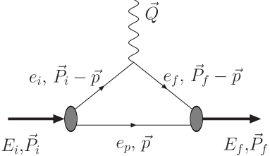
Figure 1: Diagram showing the interaction with an external probe: the kinematical definitions refer to those used for the calculation of form factors in an instant-form approach, as described in the text. The thick external lines may represent a single-particle (triangle Feynman diagram case) or a two-body system (scattering on a bound state).

3.1.1 Vector form factors

For our purpose, we use a current directly suggested by the equation of motion, Eq. (2), where the four-vector dependence on the momenta, $P_{f}^{\mu}+P_{i}^{\mu}$, is factored out in agreement with current conservation for an elastic process (or gauge invariance) and Lorentz covariance. In this way, we account implicitly for some interaction (two-body) currents. As for the expression of the elastic form factor in terms of wave functions, we require that, at $\vec{Q}=0$, it is identical to the scalar product ensuring the orthogonality of states with different eigenvalues. For an instant-form calculation, the expression of the current thus reads:

$$\sqrt{2\,E_{f}\;2\,E_{i}}\;\langle f|J^{\mu}|i\rangle = (P_{f}^{\mu}+P_{i}^{\mu})\;F_{1}(Q^{2})$$ (33)

$$= (P_{f}^{\mu}+P_{i}^{\mu})\int\frac{d\vec{p}}{(2\,\pi)^{3}}\;\Phi(\vec{P}_{f}-\vec{p},\vec{p}\,)\;\Phi(\vec{P}_{i}-\vec{p},\vec{p}\,),$$

where $\vec{p}$ now refers to the spectator particle (see Fig. 1 for a schematical representation of the process and definition of the kinematics). Corresponding to this notation, we introduce the on-mass shell energies of the interacting constituents in the initial and final states, $e_{i}=\sqrt{m^{2}+(\vec{P}_{i}-\vec{p})^{2}}$ and $e_{f}=\sqrt{m^{2}+(\vec{P}_{f}-\vec{p})^{2}}$. At this point, two features are to be noticed.

First, using Eqs. (15) and (24), one can verify that the form factor at zero-momentum transfer as defined by Eq. (33), $F_{1}(0)$, is independent of the momentum, $\vec{P}$. This result, which is not a priori guaranteed, is in complete agreement with the same independence that we require for the mass spectrum when solving Eq. (2) in the instant-form approach.

Second, for non-zero-momentum transfers, one can imagine to introduce an extra factor in the integrand of Eq. (33) such as $(e_{f}+e_{i})/\sqrt{4\,e_{f}\;e_{i}}$. This factor, which is close to 1 in most kinematical configurations of interest, can be motivated for some part. Examination of the expression of the complete matrix element for a “zero-range” interaction shows however that other factors involving the same order of numerical uncertainty should be considered. These various corrections partly originate from the quantum mechanics character of the approach used here, which prevents one from blindly relying on the underlying field-theory model. Some of them affect the single-particle current while other ones, energy dependent, can be cast into the form of two-body currents. All of them, most often, are required to ensure Lorentz covariance or equivalence with other approaches such as an “exact” calculation of form factors or a different relativistic quantum mechanics approach. In the present work, since we are mostly interested in the gross features of form factors calculated from a single-particle current in different approaches, the many-body contributions will not be considered in detail. Anticipating on later discussions, we introduce the corrections to the single-particle current as follows:

$$\sqrt{2\,E_{f}\;2\,E_{i}}\;\langle f|J^{\mu}|i\rangle=(P_{f}^{\mu}+P_{i}^{\mu})\int\frac{d\vec{p}}{(2\,\pi)^{3}}\;\Phi(\vec{P}_{f}-\vec{p},\vec{p}\,)\;\Phi(\vec{P}_{i}-\vec{p},\vec{p}\,)$$

$$\times\frac{e_{f}+e_{i}}{\sqrt{4\,e_{f}\;e_{i}}}\;\frac{2\,\sqrt{e_{f}+e_{p}}\,\sqrt{e_{i}+e_{p}}}{e_{f}+e_{i}+2\,e_{p}}.$$ (34)

The first correction factor has its origin in the elementary coupling of a photon to constituents. The second one looks arbitrary at this point. Combined with factors present in the $\Phi(\vec{P}-\vec{p},\vec{p})$ function, it allows one to recover the expression of the diagram of Fig. 1 in the limits $E_{i}=e_{i}+e_{p},\;E_{f}=e_{f}+e_{p}$, which suppresses Z-type contributions. The overall correction factor is 1 at zero-momentum transfer, ensuring that $F_{1}(0)$, remains independent of the momentum, $\vec{P}$. Relaxing the condition that the contribution of the above time-ordered diagram be recovered, one can imagine to introduce extra factors in Eq. (34), accounting for two-body currents, whose interaction character can be transformed away in the case $E_{i}=E_{f}$. An example of such a factor is suggested by the consideration of the infinite boson-mass model (see expression of $F_{1}(Q^{2})$ in Eq. (48) below). Written as:

$$c.f.(E_{i}=E_{f})=\frac{(e_{f}+e_{i}+2\,e_{p})^{2}}{(e_{f}+e_{p})\,(e_{i}+e_{p})}\;\frac{e_{f}\;e_{i}}{(e_{f}+e_{i})^{2}}\;,$$ (35)

this factor is equal to 1 at zero momentum transfer, ensuring that $F_{1}(0)$, remains independent of the momentum, $\vec{P}$, as above.

3.1.2 Scalar form factors

In calculating form factors relative to a scalar probe, we cannot rely on constraints such as current conservation or a minimal coupling principle to determine the expression of the operator entering the matrix element. It is however reasonable at least to require that the form factor at zero-momentum transfer be independent of the total momentum, $\vec{P}$, consistently with the similar independence for the spectrum of Eq. (2) in the instant-form approach. Assuming that the form factor is the same as the charge one in the non-relativistic limit, one immediately gets a possible expression:

$$\sqrt{2\,E_{f}\;2\,E_{i}}\;\langle f|S|i\rangle =$$

$$4\,m\;F_{0}(Q^{2}) = 4\,m\;\int\frac{d\vec{p}}{(2\,\pi)^{3}}\;\Phi(\vec{P}_{f}-\vec{p},\vec{p}\,)\;\Phi(\vec{P}_{i}-\vec{p},\vec{p}\,),$$ (36)

which involves the same integral as for the current probe, Eq. (33).

In comparing the ratio of the scalar and charge form factors obtained from Eqs. (33) and (36) with the one obtained from an “exact” calculation (Wick-Cutkosky model for a zero-mass boson or Feynman triangle diagram for an infinite mass), we found it is too small at low $Q^{2}$ and too large at high $Q^{2}$. The discrepancy is moderate and does not go beyond a factor 2. However, when looking at the expression of the matrix elements, Eqs. (33) and (36), it is found that the ratio of the scalar and charge form factors is not recovered in the non-interacting case at zero-momentum transfer. This ratio, $(e_{f}+e_{f}+2\,e_{p})/[2\,(e_{f}+e_{i})]$, could be introduced in Eq. (36) but, when doing so, the independence of the scalar form factor of the momentum $\vec{P}$ at zero-momentum transfer is lost (a factor 1.5 between $P=0$ and $P=\infty$ for the infinite boson-mass model). As far as we can see, this can be partly remedied at the expense of introducing an energy dependence in the expression of the scalar form factor so that to recover the above ratio in the free-particle case. On the other hand, corrections included in Eq. (34) should be accounted for. An improved expression of the scalar matrix element is thus given by:

$$\sqrt{2\,E_{f}\;2\,E_{i}}\;\langle f|S|i\rangle=4\,m\int\frac{d\vec{p}}{(2\,\pi)^{3}}\;\Phi(\vec{P_{f}}-\vec{p},\vec{p}\,)\;\Phi(\vec{P_{i}}-\vec{p},\vec{p}\,)$$ (37)

$$\qquad\quad\times\,\frac{\sqrt{e_{f}+e_{p}}\,\sqrt{e_{i}+e_{p}}}{\sqrt{4\,e_{f}\;e_{i}}}\;\left(1+e_{p}\;\frac{(e_{f}+e_{p})\,(e_{i}+e_{p})-E_{f}\,E_{i}}{(e_{f}+e_{p})\,(e_{i}+e_{p})\,(e_{f}+e_{i})}\;\right).$$

This expression is suggested by the analysis of the contribution of the Feynman triangle diagram (see expression below) where a tedious calculation allows one to check that the form factor at zero momentum transfer does not depend on the momentum, $\vec{P}$. In comparison with Eq. (36), it provides some enhancement of the form factor at small $Q^{2}$ and a decrease by roughly a factor 2 at the largest $Q^{2}$, both in agreement with what an “exact” calculation suggests. Most of the effect is due to the last factor in Eq. (37).

3.1.3 Expressions of form factors

The expressions of charge and scalar form factors are obtained from Eqs. (34) and (37), where wave functions $\Phi(...)$ are replaced according to Eq. (24):

$$F_{1}(Q^{2}) = \int\frac{d\vec{p}}{(2\,\pi)^{3}}\;\frac{\sqrt{e_{k_{tf}}\,e_{k_{ti}}}}{e_{p}}\;\phi_{0}(\vec{k}_{tf}^{2})\;\phi_{0}(\vec{k}_{ti}^{2})\;\frac{(e_{f}+e_{p})\,(e_{i}+e_{p})\,(e_{f}+e_{i})}{2\,e_{f}\,e_{i}\,(e_{i}+e_{f}+2\,e_{p})},$$

$$F_{0}(Q^{2}) = \int\frac{d\vec{p}}{(2\,\pi)^{3}}\;\frac{\sqrt{e_{k_{tf}}\,e_{k_{ti}}}}{e_{p}}\;\phi_{0}(\vec{k}_{tf}^{2})\;\phi_{0}(\vec{k}_{ti}^{2})\;$$ (38)

$$\times\frac{(e_{f}+e_{p})\,(e_{i}+e_{p})}{4\,e_{f}\,e_{i}}\;\left(1+e_{p}\;\frac{(e_{f}+e_{p})\,(e_{i}+e_{p})-E_{f}\,E_{i}}{(e_{f}+e_{p})\,(e_{i}+e_{p})\,(e_{f}+e_{i})}\;\right).$$

The arguments in the wave functions, $\vec{k}_{ti}^{2}$ and $\vec{k}_{tf}^{2}$, read:

$$\vec{k}_{ti,f}^{2}=\left(\frac{1}{2}\vec{P}_{i,f}-\vec{p}\,\right)^{2}-\left(\frac{\vec{P}_{i,f}\cdot(\frac{1}{2}\vec{P}_{i,f}-\vec{p}\,)}{(e_{P_{i,f}-p}+e_{p})}\right)^{2}.$$

The appearance of quantities such as $(e_{i}+e_{p})$ or $(e_{f}+e_{p})$ in Eq. (38) is unusual. It makes sense however if one looks at the expression of the wave function $\phi_{0}(\vec{k}_{ti}^{2})$, which involves a term $(E_{i}^{2}-(e_{i}+e_{p})^{2})^{-1}=(E_{i}-e_{i}-e_{p})^{-1}\;(E_{i}+e_{i}+e_{p})^{-1}$, see Eq. (2). Up to a factor 2, this extra quantity just cancels the second non-singular factor in the limit $E_{i}\rightarrow e_{i}+e_{p}$. As for the quantity $(e_{f}+e_{i})/(e_{i}+e_{f}+2\,e_{p})$ in the expression of $F_{1}(Q^{2})$, it represents the ratio of the coupling of the photon to the vector current, a priori expected, to the term $E_{i}+E_{f}$ which is factored out and is equal to $e_{i}+e_{f}+2\,e_{p}$ in the free particle case. Despite the factorization of the quantity $(P_{f}^{\mu}+P_{i}^{\mu})$ in Eq. (34), our expression of the charge form factor thus keeps some track of the genuine coupling. Not surprisingly, the above ratio is absent in the expression of the form factor relative to a scalar probe, $F_{0}(Q^{2})$.

The expressions in the Breit frame are obtained from Eq. (38) by making the replacements $e_{i}=e_{-\frac{Q}{2}-p}$ and $e_{f}=e_{\frac{Q}{2}-p}$. Specializing here and below to a momentum transfer along the $z$ axis, the arguments of the wave functions are then given by:

$$\vec{k}_{ti}^{2} = p^{2}_{x}+p^{2}_{y}+(p_{z}+Q/4)^{2}\;\left(1-\frac{(Q/2)^{2}}{(e_{-\frac{Q}{2}-p}+e_{p})^{2}}\right),$$

$$\vec{k}_{tf}^{2} = p^{2}_{x}+p^{2}_{y}+(p_{z}-Q/4)^{2}\;\left(1-\frac{(Q/2)^{2}}{(e_{\frac{Q}{2}-p}+e_{p})^{2}}\right).$$ (39)

We now present the expressions that form factors take in other approaches.

3.2 Expressions of form factors in other approaches

3.2.1 Point-form calculation

For the form factors in the point form, we start from currents similar to the ones used to derive the expressions of the form factors in the instant form, Eqs. (33) and (36). In doing so, we want to avoid some major bias in the comparison of results for different forms. Beginning with the charge form factor, we notice that each factor in the instant-form expression of $F_{1}(Q^{2})$, Eq. (38), has an obvious counterpart in a covariant calculation:

$$\frac{1}{2\,e} \rightarrow \int dp^{0}\delta(p^{2}-m^{2})\;\theta(\lambda_{i}\cdot p),$$

$$2\,\sqrt{e_{k_{tf}}\;e_{k_{ti}}} \rightarrow \Big{(}(p_{f}+p)^{2}\;(p_{i}+p)^{2}\Big{)}^{1/4}\;(=2\,\sqrt{\lambda_{f}\cdot p\;\;\lambda_{i}\cdot p}\;),$$

$$e_{i}+e_{p} \rightarrow \lambda_{i}\cdot(p_{i}+p),$$

$$e_{f}+e_{i}+2\,e_{p} \rightarrow (p_{f}+p_{i}+2\,p)\cdot(\lambda_{i}+\lambda_{f})\,.$$ (40)

We notice that, in place of the second expression above, a different factor, $\;p\cdot(\lambda_{i}+\lambda_{f})$, was used in an earlier version of this work. It was introduced in the integrand for the $F_{1}(Q^{2})$ form factor, without reference to Eq. (38), so that to ensure that the current be unchanged at $Q=0$. Compared with the factor, $(e_{f}+e_{i}+2\,e_{p})$, it was found to play a relatively minor role. The choice adopted in Eq. (40) is better founded however. In considering the scalar form factor, $F_{0}(Q^{2})$, we continue to assume that the ratio of its integrand to that one for the charge form factor is given by $(e_{f}+e_{i}+2\,e_{p})/[2\,(e_{f}+e_{i})]$. This one turns out to be important in order to get the ratio of the scalar and charge form factors, $F_{0}(Q^{2})/F_{1}(Q^{2})$, approximately right in the limit of large momentum transfers or large binding. The extra correction introduced in the instant-form scalar form factor, Eq. (37), in order to make it independent of the total momentum, $\vec{P}_{i,f}$, at zero momentum transfer, at least in the infinite-mass boson case, is not needed here since the present formalism is covariant in any case. The above requirements together with Lorentz invariance and the condition of recovering the expression of the free current in the small coupling limit are then sufficient to provide a minimal expression for the form factors:

$$F_{1}(Q^{2})=\frac{1}{(2\pi)^{3}}\int d^{4}p\,d^{4}p_{f}\,d^{4}p_{i}\,d\eta_{f}\,d\eta_{i}\;$$

$$\times\,\;\Big{(}(p_{f}+p)^{2}\,(p_{i}+p)^{2}\Big{)}^{1/4}\;\phi_{0}\Big{(}(\frac{p_{f}-p}{2})^{2}\Big{)}\;\phi_{0}\Big{(}(\frac{p_{i}-p}{2})^{2}\Big{)}$$

$$\times\,\delta(p^{2}-m^{2})\;\delta(p^{2}_{f}-m^{2})\;\delta(p^{2}_{i}-m^{2})\,\delta^{4}(p_{f}+p-\lambda_{f}\eta_{f})\;\delta^{4}(p_{i}+p-\lambda_{i}\eta_{i})$$

$$\times\,\theta(\lambda_{f}\cdot p_{f})\;\theta(\lambda_{f}\cdot p)\;\theta(\lambda_{i}\cdot p)\;\theta(\lambda_{i}\cdot p_{i})\,\;\;\lambda_{f}\cdot(p_{f}+p)\;\;\lambda_{i}\cdot(p_{i}+p)\;$$

$$\times\,\frac{2\,(p_{f}+p_{i})\cdot(\lambda_{f}+\lambda_{i})}{(p_{f}+p_{i}+2\,p)\cdot(\lambda_{f}+\lambda_{i})},$$

$$F_{0}(Q^{2})=\frac{1}{(2\pi)^{3}}\int d^{4}p\,d^{4}p_{f}\,d^{4}p_{i}\,d\eta_{f}\,d\eta_{i}\;$$

$$\times\,\;\Big{(}(p_{f}+p)^{2}\,(p_{i}+p)^{2}\Big{)}^{1/4}\;\phi_{0}\Big{(}(\frac{p_{f}-p}{2})^{2}\Big{)}\;\phi_{0}\Big{(}(\frac{p_{i}-p}{2})^{2}\Big{)}$$

$$\times\,\delta(p^{2}-m^{2})\;\delta(p^{2}_{f}-m^{2})\;\delta(p^{2}_{i}-m^{2})\,\delta^{4}(p_{f}+p-\lambda_{f}\eta_{f})\;\delta^{4}(p_{i}+p-\lambda_{i}\eta_{i})$$

$$\times\,\theta(\lambda_{f}\cdot p_{f})\;\theta(\lambda_{f}\cdot p)\;\theta(\lambda_{i}\cdot p)\;\theta(\lambda_{i}\cdot p_{i})\,\;\;\lambda_{f}\cdot(p_{f}+p)\;\;\lambda_{i}\cdot(p_{i}+p)\;.$$

Notations, which evidence explicitly the Lorentz invariance, have been explained in Ref. [11]. Let us only mention here that the four-vectors $\lambda_{i,f}^{\mu}$ are proportional to the total momenta $P_{i,f}^{\mu}$. On the other hand, the $\delta(...)$, when integrated over the $\eta_{i,f}$ variables, imply relations between momenta similar to Eq. (4), but with different $\lambda^{\mu}$. The same $\delta(...)$ functions imply relations such as

$$\eta_{i}=2\,\lambda_{i}\cdot p=2\,\lambda_{i}\cdot p_{i}=\sqrt{(p_{i}+p)^{2}}\;,$$

allowing one to rewrite Eqs. (3.2.1) in various forms. Up to the notations and the last factor introduced in the expression of the charge form factor, these equations could be obtained from applying methods used in Refs. [23, 24].

In the Breit frame, the above expressions read:

$$F_{1}(Q^{2}) = \frac{1+v^{2}}{\sqrt{1-v^{2}}}\;\int\frac{d\vec{p}}{(2\pi)^{3}}\;\phi_{0}(\vec{k}_{tf}^{2})\;\phi_{0}(\vec{k}_{ti}^{2})\;\sqrt{1-\Big{(}\frac{\vec{p}\cdot\vec{v}}{e_{p}}\Big{)}^{2}}\;,$$

$$F_{0}(Q^{2}) = \frac{1}{\sqrt{1-v^{2}}}\;\int\frac{d\vec{p}}{(2\pi)^{3}}\;\phi_{0}(\vec{k}_{tf}^{2})\;\phi_{0}(\vec{k}_{ti}^{2})\;\sqrt{1-\Big{(}\frac{\vec{p}\cdot\vec{v}}{e_{p}}\Big{)}^{2}}\;,$$ (42)

where

$$\vec{k}_{ti}^{2}=p^{2}_{x}+p^{2}_{y}+\left(\frac{p_{z}+v\,e_{p}}{\sqrt{1-v^{2}}}\right)^{2},\;\;\;\;\vec{k}_{tf}^{2}=p^{2}_{x}+p^{2}_{y}+\left(\frac{p_{z}-v\,e_{p}}{\sqrt{1-v^{2}}}\right)^{2},$$ (43)

and $v^{2}=Q^{2}/(4\,M^{2}+Q^{2})$ for the elastic case considered throughout this work. Expressions for the arguments that can be more easily compared to other ones in different approaches are as follows:

$$\vec{k}_{ti}^{2}=p_{x}^{2}+p_{y}^{2}+\left(\frac{p_{z}}{\sqrt{1-v^{2}}}+\frac{Q}{4}\;\frac{2\,e_{p}}{M}\right)^{2},$$

$$\vec{k}_{tf}^{2}=p_{x}^{2}+p_{y}^{2}+\left(\frac{p_{z}}{\sqrt{1-v^{2}}}-\frac{Q}{4}\;\frac{2\,e_{p}}{M}\right)^{2}.$$ (44)

3.2.2 Front-form calculation

Expressions for the form factors in the front form have been given in different places for the standard configuration $q^{+}=q^{0}+q^{z}=0$. We give them here, using the notations of the work by Karmanov and Smirnov [3] and taking care that the wave function entering this calculation involves an extra factor, see Eq. (23):

$$F_{1}(Q^{2}) = \frac{1}{(2\,\pi)^{3}}\int d^{2}R\int_{0}^{1}\frac{dx}{2x(1-x)}\;\tilde{\phi}(\vec{R}^{2},x)\;\tilde{\phi}((\vec{R}-x\vec{Q})^{2},x),$$

$$F_{0}(Q^{2}) = \frac{1}{(2\,\pi)^{3}}\int d^{2}R\int_{0}^{1}\frac{dx}{4x(1-x)^{2}}\;\tilde{\phi}(\vec{R}^{2},x)\;\tilde{\phi}((\vec{R}-x\vec{Q})^{2},x),$$ (45)

where $\tilde{\phi}(\vec{R}^{2},x)$ is obtained from $\tilde{\phi}(\vec{k}^{2})$, Eq. (23), by the following replacement of the argument:

$$\vec{k}^{2}=\frac{m^{2}+\vec{R}^{2}}{4\,x\,(1-x)}-m^{2}=\vec{R}^{2}+\;\frac{m^{2}+\vec{R}^{2}}{4\,x\,(1-x)}\;(1-2\,x)^{2}.$$ (46)

The expression of the arguments entering the wave functions in Eq. (45), also given in Eq. (46) for a particular case, can be recovered from an equation identical to Eq. (12) together with the relation that momenta $\vec{p}_{1}$, $\vec{p}_{2}$ and the total momentum $\vec{P}$ of the system fulfill in the front-form approach. This one is given by Eq. (4), where the ratio $\vec{\lambda}/\lambda^{0}$ is replaced by a unit vector $\vec{n}$. The calculation, which is somewhat tedious, is performed for a kinematical configuration where $E_{i}=E_{f}\;(\vec{Q}\perp(\vec{P}_{i}+\vec{P}_{f}))$ and $(\vec{P}_{i}+\vec{P}_{f})\parallel\vec{n}$. The momentum of the interacting particle is first replaced in terms of the spectator one, using the relation between momenta defined above. The components of this momentum perpendicular and parallel to $\vec{n}$ are then expressed in terms of the $\vec{R}$ and $x$ variables. A last translation, $\vec{R}\rightarrow\vec{R}-x\,\vec{Q}/2$, allows one to get arguments of the wave functions as shown in Eq. (45). Calculations in a configuration different from the above one are possible but rarely mentioned in the literature. They are expected to depend significantly on interaction effects and should involve sizeable contributions from two-body currents.

3.2.3 “Exact” calculations

In all present cases, calculations of form factors, that can be considered “exact”, as far as the implementation of relativity is concerned, are available. They can be obtained with a limited amount of work in the zero-mass boson case (Wick-Cutkosky model [14, 15]) and the infinite-mass one. In the case of a finite-mass boson, much more work is required. Some results have been recently obtained by Sauli and Adam for momentum transfers up to $Q^{2}=6\,m^{2}$ [38, 39]. Obviously, the consideration of scalar particles greatly simplifies the task but it also avoids to deal with models that could evidence critical values for the coupling constant [40]. Such a feature could significantly complicate the comparison with other approaches.

In the case of the Wick-Cutkosky model, some details about the calculation of form factors and their expressions that we use have been given in Refs. [11, 41]. For the infinite-mass boson case, a few details can be found in Ref. [12]. The corresponding expressions are given by:

$$F_{1}(Q^{2}) = \frac{1}{N}\;\int_{0}^{1}dx\;(1-x)\;\frac{1}{Q\,\sqrt{m^{2}-M^{2}\,x(1-x)+Q^{2}\,x^{2}/4}}\;$$

$$\times\,\log\left(\frac{\sqrt{m^{2}-M^{2}\,x(1-x)+Q^{2}\,x^{2}/4}+Q\,x/2}{\sqrt{m^{2}-M^{2}\,x(1-x)+Q^{2}\,x^{2}/4}-Q\,x/2}\right),$$

$$F_{0}(Q^{2}) = \frac{1}{N}\;\int_{0}^{1}dx\;\frac{1}{2}\;\frac{1}{Q\,\sqrt{m^{2}-M^{2}\,x(1-x)+Q^{2}\,x^{2}/4}}\;$$ (47)

$$\times\,\log\left(\frac{\sqrt{m^{2}-M^{2}\,x(1-x)+Q^{2}\,x^{2}/4}+Q\,x/2}{\sqrt{m^{2}-M^{2}\,x(1-x)+Q^{2}\,x^{2}/4}-Q\,x/2}\right),$$

where $N$ is given by Eq. (31). Alternative expressions can be obtained by integrating over the time component of the spectator particle in the original Feynman diagram. In the Breit frame, they read:

$$F_{1}(Q^{2}) = \frac{16\,\pi^{2}}{N}\int\frac{d\,\vec{p}}{(2\,\pi)^{3}}$$

$$\frac{(e_{f}+e_{i}+2\,e_{p})}{2\,e_{p}\,(e_{f}+e_{i})\,(E^{2}-(e_{f}+e_{p})^{2})\,(E^{2}-(e_{i}+e_{p})^{2})},$$

$$F_{0}(Q^{2}) = \frac{16\,\pi^{2}}{N}\int\frac{d\,\vec{p}}{(2\,\pi)^{3}}$$ (48)

$$\frac{(e_{f}+e_{p})\,(e_{i}+e_{p})\,(e_{f}+e_{i}+e_{p})-e_{p}\,E^{2}}{4\,e_{f}\,e_{i}\,e_{p}\,(e_{f}+e_{i})\,(E^{2}-(e_{f}+e_{p})^{2})\,(E^{2}-(e_{i}+e_{p})^{2})},$$

with $E=\sqrt{M^{2}+(\vec{Q}/2)^{2}},\;e_{i}=\sqrt{m^{2}+(\vec{p}+\vec{Q}/2)^{2}},\;e_{f}=\sqrt{m^{2}+(\vec{p}-\vec{Q}/2)^{2}}$.

In the limit of a vanishing total mass ($M=0$), analytical expressions of the above form factors can be obtained. As they may be useful either to get an insight on their asymptotic behavior or, more practically, to remedy the difficulty to integrate the most delicate part in Eqs. (48) in the finite-mass case, they are given here:

$$F_{1}(Q^{2})_{M=0}=\frac{12\,m^{2}}{Q^{2}}\;\Bigg{\{}1-\frac{4\,m^{2}}{Q^{2}}$$

$$\qquad+\left(\log\Big{[}\sqrt{1+Q^{2}/(4\,m^{2})}+Q/(2\,m)\Big{]}-\frac{2\,m}{Q}\sqrt{1+Q^{2}/(4\,m^{2})}\right)^{2}\Bigg{\}},$$

$$F_{0}(Q^{2})_{M=0}=\frac{6\,m^{2}}{Q^{2}}\;\left(\log\Big{[}\sqrt{1+Q^{2}/(4\,m^{2})}+Q/(2\,m)\Big{]}\right)^{2}.$$ (49)

3.2.4 Galilean-covariant calculation

Expressions of form factors with a Galilean boost are well known. They are nevertheless displayed here to better emphasize the differences or similarities with expressions involving relativistic boosts. Wave functions used in this calculation are obtained from the interaction model, Eq. (17), the normalization factors, $1/\sqrt{e_{k}}$, appearing in Eq. (5) being replaced by $1/\sqrt{m}$, which is consistent with the Galilean character of the boost made here. The general expressions are given by:

$$F_{1}(Q^{2})=F_{0}(Q^{2})=\int\frac{d\vec{p}}{(2\,\pi)^{3}}\;\phi_{f}(\vec{k}_{tf}^{2})\;\phi_{i}(\vec{k}_{ti}^{2}),$$ (50)

with

$$\vec{k}_{ti}^{2}=\left(\frac{1}{2}\vec{P}_{i}-\vec{p}\right)^{2},\;\;\;\;\vec{k}_{tf}^{2}=\left(\frac{1}{2}\vec{P}_{f}-\vec{p}\right)^{2}.$$ (51)

Galilean invariance of these form factors holds provided that the boost is performed according to the premises of this symmetry, i.e. by discarding corrections to the mass due to binding energy and other $1/m$ terms.

In the Breit frame, with $\vec{Q}$ along the $z$ axis, the above arguments read:

$$\vec{k}_{ti}^{2}=p^{2}_{x}+p^{2}_{y}+\left(p_{z}+\frac{Q}{4}\right)^{2},\;\;\;\;\vec{k}_{tf}^{2}=p^{2}_{x}+p^{2}_{y}+\left(p_{z}-\frac{Q}{4}\right)^{2}.$$ (52)

3.3 Relations and comments

The expressions of form factors given above for different formalisms have been derived independently, keeping however in mind that well determined limits should be recovered in some cases.

It is first noticed that expressions for the form factors in the instant form allow one to recover the front-form ones in the kinematical configuration where the average momentum carried by the system, $\vec{\bar{P}}$, goes to infinity, which defines a specific axis, while the momentum transfer, $\vec{Q}=\vec{P}_{f}-\vec{P}_{i}$, remains orthogonal to the direction so defined. The result holds for both charge and scalar form factors and is independent of the dynamics. It evidently relies on the various factors introduced in the definition of the form factors but also on the precise expression taken by the arguments entering the wave function, Eq. (3.1.3), thus providing a check of their relevance.

A second relation concerns the infinite-mass boson model (“zero-range” interaction). It is found that form factors calculated with the front-form expressions are identical to the ones directly obtained from the Feynman triangle diagram. This can be shown by inserting in Eq. (45) the appropriate wave function. This one, which can be obtained from Eq. (23) together with Eq. (29), takes a simple form, $\tilde{\phi}(\vec{k}^{2})\propto 1/(m^{2}-M^{2}/4+\vec{k}^{2})$. As there is a reduced dependence on the interaction (“zero-range” one) and on the current (contributions of pair-terms in other formalisms are suppressed here), the present result represents a severe test on the implementation of boost effects.

Our third comment, which complements the previous one, concerns the expression taken by the argument of the wave function entering the calculation of form factors when boost effects are accounted for. Looking at the transformation of the minimal factor $1/(m^{2}-M^{2}/4+\vec{k}^{2})$, which is part of the c.m. wave function in all formalisms, it is found that our instant-form expression agrees with what the analysis of the Feynman triangle diagram indicates, Eq. (48). In the Breit frame for instance, the above factor for the initial state becomes $1/(m^{2}-M^{2}/4+\vec{k}_{ti}^{2})$ with $\vec{k}_{ti}^{2}$ given by Eq. (39), while the corresponding factor in the other case reads $1/[(e_{i}+e_{p})^{2}/4-E^{2}/4]$. Even though the expressions appear quite different, one can convince oneself, after some algebra, that they are indeed identical (Eq. (12) is especially useful). This represents another severe test on the implementation of boost effects in the calculation of form factors. Until now, we could not find any similar result when the boost-transformed $\vec{k}^{2}$ of the point-form approach, Eq. (39), is used. The appearance of the factor $1/e_{p}$ in our instant-form expression of the form factor, Eq. (38), is also worthwhile to be noticed. It is not clear that it has a general character but it appears in the expression of the form factor for an infinite-mass boson, Eq. (48), while it is absent in the point-form expressions. It is essential to describe the form factors at large $Q^{2}$, especially their log dependence.

The fourth and last comment concerns the Lorentz contraction effect. As mentioned in the introduction, we do not expect it to be accounted for by the simple replacement of the momentum transfer, $Q^{2}\rightarrow Q^{2}\,(1-v^{2})=Q^{2}/[1+Q^{2}/(4M^{2})]$, leading to a constant form factor at large $Q^{2}$. We nevertheless expect this effect to be around in some limit. Examining the expressions for the form factors in the instant form, especially the boost-transformed $\vec{k}^{2}$, Eq. (39), one sees that the quantity, $(p_{z}\pm Q/4)^{2}$, involves an extra factor which is absent for a Galilean boost and is close to the factor $1-v^{2}$. In this limit and taking into account that an extra factor $\sqrt{1-v^{2}}$ appears in the integrand of the form factor, one can reproduce the above recipe. However, the identity between the factor $1-v^{2}$ and the extra factor only holds in the low $Q^{2}$ and small binding limits. At high $Q^{2}$, the former one tends to zero like $1/Q^{2}$ while the latter one either goes to zero like $1/Q$ (small momentum for the spectator particle) or to a constant (longitudinal momentum of the order $p_{z}\pm Q/4$). This is sufficient to make the form factor decrease when $Q^{2}$ increases. The erroneous character of the above recipe can be seen as follows. The constant form factor to which it leads at high $Q^{2}$ implies that the system in the Breit-frame has no depth along the momentum transfer. In other words, the two constituents arrive and go back together, which is not what occurs physically. The photon momentum is transferred to one constituent while the other one is not affected. This difference in the role of the two particles is accounted for by the departure from the factor $v^{2}$ evidenced by the last term in the two expressions of Eq. (39), which, moreover, differ from each other. Such a departure was found in a numerical study by Glöckle and Nogami at the lowest order in the interaction [22]. However, contrary to their conjecture that this should vanish at higher order, we believe that these differences are there and are essential to get the appropriate asymptotic behavior of form factors.

4 Presentation of the results

We present here results for elastic form factors calculated with the different expressions for the boost transformation given in the previous section. They concern the ground state of a two-body system composed of scalar particles interacting by exchanging a scalar boson. Most results have a covariant character, Lorentzian or Galilean. Only those for the instant-form approach do not have such a property. Their frame dependence will be discussed in the second part of this section.

4.1 Covariant and Breit-frame calculations

Numerical results are successively given in three tables: Table 1 for a zero-mass boson, Table 2 for a finite mass boson ($\mu=0.15\,m$) and Table 3 for an infinite one. In every case, two masses of the total system are considered corresponding to a moderately and a strongly bound system, roughly $M\simeq 1.6\,m$ and $M=0.1\,m$, respectively (the precise values are given in the table).

Table 1: Elastic scalar- and vector- form factors, $F_{1}(Q^{2})$ and $F_{0}(Q^{2})$: Results for a mass-less boson and two different total masses of the system, $M=1.568\,m$ and $0.1\,m$ ($\kappa^{2}=0.385\,m^{2}$ and $\kappa^{2}=0.9975\,m^{2}$). The table successively contains results for the instant-form boost (I.F.), for the front-form boost (F.F.), and the point-form boost (P.F.), all of them with wave function obtained from Eqs. (5) and (17), for the Wick-Cutkosky model (B.S.), and for a Coulombian wave function with a Galilean boost (Gal.). The corresponding coupling constants are given in Table 4. Asymptotic behaviors for $F_{1}(Q^{2})$ are $Q^{-4}\;\log Q$, $Q^{-4}\;\log Q$, $Q^{-8}$, $Q^{-4}\;\log Q$, and $Q^{-4}$ for I.F., F.F., P.F., B.S. and Gal., respectively. Except for a few cases, they are not reached in the range of momentum transfers shown in the table.

$Q^{2}/m^{2}$	0.01	0.1	1.0	10.0	100.0
$M=1.568\,m$
$F_{1}\;\;\;\;$I.F.	0.996	0.956	0.668	0.111	0.342-02
$F_{0}\;\;\;\;$I.F.	1.237	1.182	0.787	0.106	0.253-02
$F_{1}\;\;\;\;$F.F.	0.995	0.954	0.657	0.102	0.302-02
$F_{0}\;\;\;\;$F.F.	1.062	1.014	0.675	0.091	0.222-02
$F_{1}\;\;\;\;$P.F.	0.993	0.928	0.507	0.195-01	0.167-04
$F_{0}\;\;\;\;$P.F.	0.992	0.919	0.464	0.130-01	0.087-04
$F_{1}\;\;\;\;$B.S.	0.996	0.962	0.705	0.139	0.50-02
$F_{0}\;\;\;\;$B.S.	1.123	1.080	0.767	0.132	0.39-02
$F_{1}=F_{0}\;{\rm Gal.}$	0.997	0.968	0.740	0.145	0.337-02
$M=0.1\,m$
$F_{1}\;\;\;\;$I.F.	0.998	0.979	0.818	0.270	0.156-01
$F_{0}\;\;\;\;$I.F.	1.496	1.456	1.138	0.279	0.116-01
$F_{1}\;\;\;\;$F.F.	0.998	0.977	0.804	0.251	0.142-01
$F_{0}\;\;\;\;$F.F.	1.120	1.092	0.866	0.227	0.102-01
$F_{1}\;\;\;\;$P.F.	0.431	0.806-02	0.393-05	0.682-09	0.95-13
$F_{0}\;\;\;\;$P.F.	0.360	0.470-02	0.200-05	0.342-09	0.47-13
$F_{1}\;\;\;\;$B.S.	0.998	0.983	0.848	0.338	0.283-01
$F_{0}\;\;\;\;$B.S.	1.247	1.222	1.016	0.338	0.217-01
$F_{1}=F_{0}\;{\rm Gal.}$	0.999	0.988	0.886	0.378	0.189-01

Table 2: Elastic scalar- and vector- form factors, $F_{1}(Q^{2})$ and $F_{0}(Q^{2})$: Same as for Table 1 but for a boson mass, $\mu=0.15\,m$. The two total masses are $M=1.6\,m$ and $0.1\,m$. The corresponding coupling constants are $g^{2}/4\pi=1.915$ and $3.392$ for the interaction model given by Eqs. (5) and (17), and $g^{2}/4\pi=1.487$ and $2.289$ for model the simple Yukawa potential. Bethe-Salpeter results are from refs. [38, 39] (see comments in the text).

$Q^{2}/m^{2}$	0.01	0.1	1.0	10.0	100.0
$M=1.6\,m$
$F_{1}\;\;\;\;$I.F.	0.997	0.968	0.741	0.171	0.68-02
$F_{0}\;\;\;\;$I.F.	1.241	1.198	0.877	0.164	0.50-02
$F_{1}\;\;\;\;$F.F.	0.997	0.966	0.729	0.158	0.61-02
$F_{0}\;\;\;\;$F.F.	1.084	1.046	0.762	0.141	0.44-02
$F_{1}\;\;\;\;$P.F.	0.995	0.948	0.608	0.381-01	0.41-04
$F_{0}\;\;\;\;$P.F.	0.994	0.939	0.5580	0.255-01	0.22-04
$F_{1}\;\;\;\;$B.S.	(0.996)	(0.961)	(0.697)	(0.119)	(0.27-02)
$F_{1}=F_{0}\;{\rm Gal.}$	0.998	0.976	0.796	0.209	0.63-02
$M=0.1\,m$
$F_{1}\;\;\;\;$I.F.	0.999	0.984	0.859	0.349	0.263-01
$F_{0}\;\;\;\;$I.F.	1.496	1.464	1.201	0.366	0.195-01
$F_{1}\;\;\;\;$F.F.	0.998	0.982	0.844	0.324	0.241-01
$F_{0}\;\;\;\;$F.F.	1.150	1.126	0.931	0.298	0.173-01
$F_{1}\;\;\;\;$P.F.	0.509	0.137-01	0.76-05	0.137-08	0.19-12
$F_{0}\;\;\;\;$P.F.	0.425	0.080-01	0.39-05	0.069-08	0.10-12
$F_{1}=F_{0}\;{\rm Gal.}$	0.999	0.990	0.908	0.451	0.293-01

Table 3: Elastic scalar- and vector- form factors, $F_{1}(Q^{2})$ and $F_{0}(Q^{2})$: Same as for Table 1 but for an infinite-mass boson. The two total masses are $M=1.6\,m$ and $0.1\,m$ ($\kappa^{2}=0.36\,m^{2}$ and $\kappa^{2}=0.9975\,m^{2}$). The wave function used in the I.F., F.F. and P.F. cases is issued from Eq. (5). Asymptotic behaviors for $F_{1}(Q^{2})$ are $Q^{-2}\;(\log Q)^{2}$, $Q^{-2}\;(\log Q)^{2}$, $Q^{-4}$, $Q^{-2}\;(\log Q)^{2}$, and $Q^{-1}$ for I.F., F.F., P.F., B.S. and Gal., respectively. Except for a few cases, they are not reached for the range of momentum transfers shown in the table. Part of the results were presented in [12].

$Q^{2}/m^{2}$	0.01	0.1	1.0	10.0	100.0
$M=1.6\,m$
$F_{1}\;\;\;\;$I.F.	0.999	0.990	0.917	0.594	0.208
$F_{0}\;\;\;\;$I.F.	1.325	1.309	1.176	0.658	0.187
$F_{1}\;\;\;\;$F.F.	0.999	0.989	0.908	0.566	0.191
$F_{0}\;\;\;\;$F.F.	1.325	1.309	1.176	0.659	0.187
$F_{1}\;\;\;\;$P.F.	0.999	0.986	0.871	0.353	0.207-01
$F_{0}\;\;\;\;$P.F.	0.998	0.976	0.800	0.236	0.108-01
$F_{1}\;\;\;\;$B.S.	0.999	0.989	0.908	0.566	0.191
$F_{0}\;\;\;\;$B.S.	1.325	1.309	1.176	0.659	0.187
$F_{1}=F_{0}\;$Gal.	0.999	0.994	0.947	0.699	0.320
$M=0.1\,m$
$F_{1}\;\;\;\;$I.F.	0.999	0.996	0.963	0.759	0.343
$F_{0}\;\;\;\;$I.F.	1.498	1.487	1.389	0.920	0.320
$F_{1}\;\;\;\;$F.F.	0.999	0.995	0.954	0.723	0.315
$F_{0}\;\;\;\;$F.F.	1.498	1.487	1.389	0.920	0.320
$F_{1}\;\;\;\;$P.F.	0.839	0.222	0.82-02	0.141-03	0.20-05
$F_{0}\;\;\;\;$P.F.	0.699	0.130	0.42-02	0.071-03	0.10-05
$F_{1}\;\;\;\;$B.S.	0.999	0.995	0.954	0.723	0.315
$F_{0}\;\;\;\;$B.S.	1.498	1.487	1.389	0.920	0.320
$F_{1}=F_{0}\;$Gal.	0.999	0.998	0.980	0.846	0.475

Table 4: Mass spectrum for the interaction used together with a zero-boson mass: Results are presented for two total masses of the system under consideration (in units of the constituent mass $m$). They are given for the simplest interaction, Eq. (17), for an improved interaction, Eq. (55), for the Coulombian model used together with a Galilean boost, and for the “exact” calculation (Wick-Cutkosky model). The various columns contain successively the coupling constant, the total mass for the ground state (input) and those for the first-radial excitation and $l=1$ states.

interaction	$\;\;g^{2}/4\pi\;\;\;\;$	$\;l=0\;$	$l=0^{*}$	$l=1$
$M=1.568\,m$
simplest	1.497	1.568	1.888	1.875
improved	1.314	1.568	1.897	1.891
Coulombian	1.241	1.568	1.901	1.901
“exact”	3	1.568	1.896	1.896
$M=0.1\,m$
simplest	2.750	0.10	1.668	1.615
improved	2.267	0.10	1.707	1.671
Coulombian	1.997	0.10	1.733	1.733
“exact”	1.996$\,\pi$	0.10	1.716	1.716

In each table, results employing the same wave function but different boost transformations, successively instant-form (I.F.), front-form (F.F.) and point-form (P.F.), are presented. They are followed by what can be considered as an “exact” calculation, and a non-relativistic one, characterized by a Galilean boost.

As mentioned in Sect. 2, instant-form, front-form and point-form calculations can be performed from a unique wave function, but with appropriate boost transformations. Being interested in the ground state of a two-body system, it is natural to require that the binding energy of this state be reproduced. This determines the unique parameter which enters an interaction like Eq. (17), namely the coupling constant which is given in Table 4 together with other data. This interaction model is used for results presented in Tables 1 and 2. As will be seen below, this provides in some cases (I.F. and F.F.) results that are not too far from the “exact” ones. A possibility to improve them in relation with a better account of the spectrum of our “exact” model will be discussed at the end of the section.

Concerning “exact” calculations (B.S.), there are some results in the zero-mass case (Wick-Cutkosky model). These ones together with the relevant expressions for the form factors have been obtained elsewhere [11, 41]. They correspond to the couplings $\alpha=3$ and $\alpha=1.996\,\pi$, which lead to the total mass $M=1.568\,m$ and $M=0.10\,m$. In this case, we could have considered the very extreme case of a zero mass, $\alpha=2\,\pi$. However, while most results are not sensitive to the precise value (0.5% at the largest $Q^{2}$ values considered here), those for the point-form approach are, requiring to take a non-zero finite value. These mass values are the ones used in the fitting of the interaction strength in the other models. There are also “exact” calculations in the infinite-mass boson case. Results are uniquely determined by the knowledge of the mass of the system, $M$. Finally, tentative results, given in parentheses in Table 2, have been recently obtained by Sauli and Adam in the finite-mass boson cases ($F_{1}$, $M=1.6\,m$) [38, 39]. Comparing these results with the instant- or front-form ones shows that they are relatively lower than what a similar comparison for our zero or infinite boson-mass calculation suggests. Examination of the method employed by these authors indicates that the interaction is implicitly cut off at high momentum, explaining the above observation.

Concerning the non-relativistic case, the wave function is obtained from an interaction model ignoring relativistic normalization factors $\sqrt{m/e_{p}}$. Such an interaction with a zero-mass boson (Coulombian potential) reproduces well the spectrum of the Wick-Cutkosky model [34]. The bulk of the effective coupling is understood and only minor adjustments are needed to fit the exact binding energy. The corresponding form factors scale like $Q^{-4}$ at high $Q^{2}$ and offer the advantage of taking an analytical expression:

$$F_{1}(Q^{2})=F_{0}(Q^{2})=\frac{1}{(1+Q^{2}/16\kappa^{2})^{2}},$$ (53)

where $\kappa^{2}=m^{2}-M^{2}/4$ (the same definition is referred to in Tables  1-3).

Finally, for each entry, we give results for the charge and scalar form factors, $F_{1}(Q^{2})$ and $F_{0}(Q^{2})$, which generally differ from each other. This can provide a deeper insight on the role of various ingredients introduced in the calculation.

In comparing the various results, we first consider the instant-form (I.F.), the front-form (F.F.) and the “exact” (B.S.) results. The reason is that they evidence most often the same trends. Beyond the gross features, the interest is in the remaining discrepancies at the level of a factor 2.

For the general features, we notice that they have the same asymptotic behavior, $Q^{-4}$ for the finite-range interaction and $Q^{-2}$ for the infinite range one. This is not always transparent from the results presented in the tables and, to verify it, one has to go to higher momentum transfers. As is seen in the particular case of the Galilean boost applied to a Coulombian-type problem, for which the analytical expression of the form factor is known, Eq. (53), the convergence to the asymptotic behavior is rather slow, confirming results obtained for instance for the three-quark system in ref. [42]. A refined analysis shows that there are corrections to this asymptotic behavior with a log dependence that enhances the form factor at high $Q^{2}$. Again, it is not easy to see it from examining the tables. The effect is actually responsible, in the finite-range interaction case, for the increase of the relativistic calculations (I.F., F.F. and B.S.) relative to the Galilean ones when going from $Q^{2}=10\,m^{2}$ to $Q^{2}=100\,m^{2}$. These results show the adequacy of the various factors and boost transformations involved in the different calculations.

The second general feature concerns the ratio of the form factors, $F_{0}$ and $F_{1}$. Compared to 1, it is larger at low $Q^{2}$, and smaller at the highest values. This results from the choice of the current, especially the introduction of a factor in Eq. (37) to account for the ratio of these form factors for the non-interacting case. Again, this is a support for the way form factors are calculated (wave functions and currents). At the largest values of $Q^{2}$, a ratio $1/2$ is expected. The dependence on log terms, which varies quite slowly, explains why this asymptotic result is hardly seen in the tables. Their effect can nevertheless be checked for instance on Eq. (49).

Besides these general common features, a detailed examination shows a few departures. The ratio, $F_{0}/F_{1}$, at low $Q^{2}$ for the instant-form calculation is larger than what is expected from the “exact” one while the front-form calculation shows the opposite trend (finite-range interaction case). This indicates that the factor introduced in Eq. (37), taken from the infinite-range interaction case, misses something. Notice that in absence of this factor, the ratio in the instant-form case would also disagree but would be smaller than the “exact” result at low $Q^{2}$. The truth is probably in between. On the other hand, the form factors in the instant and front forms tend to be smaller than the “exact” ones at high $Q^{2}$. This points to the choice of the effective interaction, which has not been optimized and will be discussed below.

It is worthwhile to notice that the front-form calculations generally compare well with the exact results. As is well known, the front-form approach ignores Z-type contributions that are implicitly included in the formalism. In absence of such contributions, the above agreement is not a surprise. This result is useful however, as there are not always “exact” results for the exchange of a finite-mass boson. The front-form calculations can then provide benchmark values.

From examining results presented in Tables 1-3, it is evident that the point-form calculations of form factors differ strikingly from all the other ones, especially in cases where a relativistic treatment is a priori required. Their fall-off is much faster and, moreover, it evidences a variation with the mass of the system opposite to all the other calculations. At small $Q^{2}$, the slope of the form factors in the point form suggests a charge or (Lorentz-) scalar radius significantly larger than in the other cases. As an analytical calculation in a particular model (Coulombian one) shows [11], this radius contains a term proportional to $1/M$, hence a radius tending to infinity when the mass $M$ goes to zero. One can also guess that the finite-mass-boson results presented here evidence a power-law behavior like $Q^{-8}$ at high $Q^{2}$, for the charge and scalar form factors. Such behaviors disagree with what is expected from the Born amplitude, which provides a $Q^{-4}$ power law. This one is approximately verified in the other cases. The difference is entirely due to the way the boost transformation is implemented in the wave function. At the places where the “exact”, instant-form and front-form calculations predict some $Q^{2}$ power law, the point-form calculations provide a $Q^{4}$ one. This property is probably related to the observation made in Ref. [23] that the momentum transfer at the interaction vertex with the external probe in the point-form approach, $(\vec{p}_{i}-\vec{p}_{f})^{2}$, does not vary like $Q^{2}$ as generally expected but rather like $Q^{2}\;(1+Q^{2}/(4\,M^{2}))$. While this affects the size of the form factors, it is noticed that the ratio of the charge and scalar form factors, $F_{1}(Q^{2})/F_{0}(Q^{2})$, turns out to be roughly correct, as a consequence of the extra factor introduced in the expression of $F_{1}(Q^{2})$ in Eq. (3.2.1). Despite some sizable differences with results presented elsewhere [11, 12], due to the inputs (currents and wave functions), the most important drawbacks, in the large $Q^{2}$ limit or in the $M\rightarrow 0$ limit, persist.

Galilean boost results, mainly given here as a simple benchmark, have already been mentioned. Contrary to what one could naively expect, they do rather well in the finite-range-interaction cases. This agreement is partly due to the fact that the current is conserved and that the Born amplitude constraint is fulfilled. The slight departure to the “exact” result in the zero-mass-boson case that appears at the highest value of $Q^{2}$ is essentially due to the log terms discussed above. In the infinite-mass-boson case, the relatively good agreement of the Galilean boost results with the other ones should be corrected by the observation that the asymptotic behavior differs, $Q^{-1}$ against $Q^{-2}\;(\log\,Q)^{2}$. This difference is due to a slower convergence of the integrals entering the calculation of the form factors. In comparison, the failure of the point-form results, which a priori should improve upon these non-relativistic calculations, appears as quite striking.

4.2 Frame dependence of the form factors in the instant form

The instant-form calculation of form factors is not covariant, though it used wave functions obtained from an equation that has this property for the mass spectrum. To recover a covariant form factor, the contribution of two-body currents is generally needed. This can be checked on the example of the triangle diagram already mentioned. In absence of such currents, whose derivation is not straightforward, the form factors in the instant form can depend on the frame in which they are calculated. Two particular frames are of interest. One assumes a boost along the momentum transfer, which includes in particular the Lab-frame case. The other one assumes a boost perpendicular to the momentum transfer (see Fig. 2 for a graphical representation). In the limit where an infinite momentum is given, it is generally expected that one should recover the front-form results. The two situations are successively considered now.

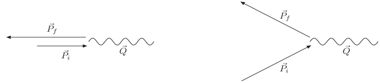
Figure 2: The left and right parts of the figure represent kinematical configurations obtained when giving some extra momentum to the system, respectively parallel and transverse to the momentum that the initial and final states have in the Breit-frame.

$\bullet$ For the parallel configuration, where, together with the momentum transfer, there is a non-zero energy transfer ($E_{i}\neq E_{f}$), it has been found that the form factors tend to decrease when going away from the Breit-frame limit with a possible saturation when the average momentum $\vec{\bar{P}}$ goes to $\infty$ (see Fig. 3 for an example in the infinite boson-mass case). The power-law behavior of the form factors does not seem to be affected. As to the reduction, it appears to increase while the total mass $M$ tends to zero. Although presented differently, the strong sensitivity of the form factors to the average momentum carried by the system has a close relation with the sensitivity to the orientation of the quantization surface found in ref. [43]. The difference with the Breit-frame results is obviously due to two-body currents, which actually can take the form of a single-particle but mass-dependent current. This can be seen on the form factors relative to the Feynman triangle diagram where analytic expressions are available. The main correction to Eqs. (38) arises from a pair-type diagram and is given by:

$$\Delta F_{1}(Q^{2})=\int\frac{d\vec{p}}{(2\,\pi)^{3}}\;\frac{\sqrt{e_{k_{tf}}\;e_{k_{ti}}}}{e_{p}}\;\phi_{0}(\vec{k}_{tf}^{2})\;\phi_{0}(\vec{k}_{ti}^{2})$$

$$\times\frac{(E_{i}-E_{f})\,(e_{i}-e_{f})\,(E_{i}+e_{i}+e_{p})\,(E_{f}+e_{f}+e_{p})}{8\,e_{i}\,e_{f}\,(E_{i}+E_{f})(e_{i}+e_{f})}$$

$$\times\frac{(E_{f}-e_{f}-e_{p})(E_{f}-E_{i}-e_{i}-e_{f})+(E_{i}-e_{i}-e_{p})(E_{i}-E_{f}-e_{i}-e_{f})}{(e_{i}+e_{f})^{2}-(E_{i}-E_{f})^{2}},$$

$$\Delta F_{0}(Q^{2})=\int\frac{d\vec{p}}{(2\,\pi)^{3}}\;\frac{\sqrt{e_{k_{tf}}\;e_{k_{ti}}}}{e_{p}}\;\phi_{0}(\vec{k}_{tf}^{2})\;\phi_{0}(\vec{k}_{ti}^{2})$$

$$\times\frac{(E_{i}-E_{f})\,(E_{i}+e_{i}+e_{p})\,(E_{f}+e_{f}+e_{p})}{16\,e_{i}\,e_{f}\,(e_{i}+e_{f})}$$

$$\times\frac{(E_{f}-e_{f}-e_{p})(E_{f}-E_{i}-e_{i}-e_{f})-(E_{i}-e_{i}-e_{p})(E_{i}-E_{f}-e_{i}-e_{f})}{(e_{i}+e_{f})^{2}-(E_{i}-E_{f})^{2}}.$$

The interaction dependence of these contributions is made clear if one notices that the factors $E_{i}-e_{i}-e_{p}$ or $E_{f}-e_{f}-e_{p}$ at the numerator of the last factor, when multiplying the wave function, can be transformed away using the mass equation, Eq. (2). Due to extra E terms, the actual dependence on the interaction is much more complicated than a linear one. In particular, the term $(E_{i}-E_{f})^{2}$ at the denominator of this last factor is essential. At large $\vec{\bar{P}}$, it tends to cancel the other term in the denominator, $(e_{i}+e_{f})^{2}$, enhancing the corresponding overall contributions. This will be lost in a limited expansion in terms of the energies. When these contributions are added to the single-particle current contribution, Eqs. (33, 37), some stability of the results on the average momentum $\vec{\bar{P}}$ is recovered. This can be seen on Fig. 3 where form factors, $F_{1}$ and $F_{0}$, are shown for $Q^{2}=10\,m^{2}$ and $M=0.10\,m$. The average momentum, $\vec{\bar{P}}$, is considered up to $50\,m$, which includes the Lab frame ($\vec{\bar{P}}\simeq 25\,m$). Notice that the example is a somewhat extreme one. The large drop off of the single-particle contribution as well as the large contribution of the two-body currents to restore the covariance has more to do with the low mass of the system than with the $Q^{2}$ value which is not excessively high. This example has been given to illustrate the role of two-body currents in a particular case where the various contributions can be dealt with easily. These ones are part of more realistic calculations with finite-range forces, for which we expect further contributions however.

A study similar to the above one could be performed in the front-form approach for the configuration, $\vec{Q}\parallel(\vec{P}_{i}+\vec{P}_{f})\parallel\vec{n}$. The results for the contribution of the single-particle current can significantly differ from those where $\vec{Q}\perp(\vec{P}_{i}+\vec{P}_{f})$, generally considered as the most reliable. These ones are recovered when one adds the contribution of two-body currents that have the same origin as those given by Eq. (LABEL:40b) for the instant-form case.

Figure 3: Dependence of form factors on the average momentum $\vec{\bar{P}}$ in the parallel configuration for $Q^{2}=10\,m^{2}$: the solid and dotted curves represent the single-particle contribution to $F_{1}$ and $F_{0}$, Eq. (38), while the dashed and dot-dashed curves include the dominant interaction effect, Eq. (LABEL:40b).

$\bullet$ For the transverse configuration, where the energies of the initial and final states remain equal ($E_{i}=E_{f}$), we did not find much sensitivity. The departure is of the order of what the omission of possible factors such as $c.f.(E_{i}=E_{f})$ given by Eq. (35), will produce. It also compares to the difference between the instant-form and the front-form results presented in Tables 1-3 (roughly 10% and 30% at most for the form factors $F_{1}$ and $F_{0}$, respectively). As expected, the instant-form results tend to the front-form ones when the average momentum, $\vec{\bar{P}}$, goes to $\infty$. The small sensitivity of the results on $\vec{\bar{P}}$ is evidently related to the orthogonality property of this vector with the momentum transfer, $\vec{Q}$, which minimizes the interference effects that plague the results for the parallel configuration. Interestingly, the introduction of the correcting factor given by Eq. (35) would remove a sizable part of the difference between the instant- and front-form calculations of $F_{1}$ and even the totality for the infinite boson-mass case.

4.3 Improved interaction

We noticed that form factors in the instant and front forms for the zero-mass boson case evidence a departure from the “exact” ones (B.S.) by a factor two or so at the highest $Q^{2}$ values. For the main purpose of this paper, which is to look at the gross features evidenced by different approaches, this is rather sufficient, knowing that one of the approaches shows orders of magnitude discrepancies. For the purpose of better checking the theoretical framework, one can nevertheless wonder about this slight discrepancy and its relation to the choice of the interaction which was taken as the simplest one possible. No attempt was made for reproducing the spectrum of the “exact” one, which is known to be close to the Coulombian one with an effective strength [34]. As departures from this spectrum are due to the normalization factors, $1/\sqrt{e_{k}}$ in Eq. (5), which are essential on the other hand, a simple way to partially correct for their effect is to compensate for the $k^{2}/m^{2}$ dependence they produce at the lowest order in this quantity. While doing so, the correction should not change the high momentum behavior of the interaction so that expectations from the consideration of the Born amplitude are still fulfilled. A better interaction could thus be:

$$V=-g^{2}\,\frac{4\,m^{2}}{\mu^{2}+(\vec{k}-\vec{k}\,^{\prime})^{2}}\;\left(1+\frac{e_{k}-m}{2\,e_{k}}+\frac{e_{k^{\prime}}-m}{2\,e_{k^{\prime}}}\right).$$ (55)

For small $k$, this interaction, including the normalization factors, looks more like a Coulombian one. We also expect its strength in this range to be closer to the latter one given in Table  4, what we indeed find. Interestingly, the force at high $k$ is enhanced by a factor 2, partly compensating the effect of the renormalization of the interaction due to retardation effects and becoming closer to the bare one. Although this result is conceivable, we have not checked whether the observation is fully relevant. This could provide a useful constraint on the derivation of the effective interaction.

Table 5: Elastic scalar- and vector- form factors, $F_{1}(Q^{2})$ and $F_{0}(Q^{2})$, with a tentatively improved interaction: Same as in Table 1, but with wave functions obtained from the interaction model, Eq. (55 ). The coupling constants corresponding to the two masses $M=1.568\,m$ and $M=0.10\,m$ are, respectively, $g^{2}/4\pi=1.314$ and $2.267$. These ones can be compared to the ones for the Wick-Cutkosky model, $g^{2}/4\pi=3$ and $g^{2}/4\pi=1.996\,\pi$ and those for the Coulombian potential used in the non-relativistic case, $g^{2}/4\pi=1.241$ and $1.997$, to which they are becoming closer. Results for the Wick-Cutkosky model are recalled.

$Q^{2}/m^{2}$	0.01	0.1	1.0	10.0	100.0
$M=1.568\,m$
$F_{1}\;\;\;\;$I.F.	0.997	0.965	0.723	0.159	0.66-02
$F_{0}\;\;\;\;$I.F.	1.247	1.201	0.860	0.153	0.48-02
$F_{1}\;\;\;\;$F.F.	0.996	0.963	0.712	0.147	0.58-02
$F_{0}\;\;\;\;$F.F.	1.079	1.039	0.742	0.132	0.43-02
$F_{1}\;\;\;\;$P.F.	0.994	0.942	0.576	0.329-01	0.37-04
$F_{0}\;\;\;\;$P.F.	0.993	0.933	0.527	0.219-01	0.19-04
$F_{1}\;\;\;\;$B.S.	0.996	0.962	0.705	0.139	0.50-02
$F_{0}\;\;\;\;$B.S.	1.123	1.080	0.767	0.132	0.39-02
$M=0.1\,m$
$F_{1}\;\;\;\;$I.F.	0.999	0.985	0.862	0.357	0.285-01
$F_{0}\;\;\;\;$I.F.	1.496	1.465	1.205	0.375	0.211-01
$F_{1}\;\;\;\;$F.F.	0.998	0.983	0.847	0.332	0.260-01
$F_{0}\;\;\;\;$F.F.	1.153	1.130	0.937	0.306	0.187-01
$F_{1}\;\;\;\;$P.F.	0.517	0.149-01	0.91-05	0.170-08	0.24-12
$F_{0}\;\;\;\;$P.F.	0.431	0.087-01	0.46-05	0.085-08	0.12-12
$F_{1}\;\;\;\;$B.S.	0.998	0.983	0.848	0.338	0.283-01
$F_{0}\;\;\;\;$B.S.	1.247	1.222	1.016	0.338	0.217-01

The form factors calculated with the above improved interaction are given in Table 5 while the spectrum of the model for the ground state, its first radial excitation and the $l=1$ state are given in Table 4. It is seen that the form factors become closer to or slightly overshoot the “exact” ones. At the same time, when it is compared to the simplest choice of the interaction, the spectrum with the improved interaction becomes better. The first radially-excited and the first $l=1$ states tend to be closer to each other and closer to the “exact” ones.

The aim of the present subsection was to provide some insight on a possible sensitivity of form factors to the effective interaction used in the calculation of wave functions. This was done by modifying the initial interaction in a manner that would be more consistent with the main features of the Wick-Cutkosky model, but we have not attempted a refined description. Considering the simultaneous improvement of the form factors at the highest $Q^{2}$ values and the position of the first radially excited state, we expect that such a refined interaction could easily remove a large part of the remaining differences. This should be checked carefully however, especially in view of doubts sometimes expressed about reproducing in relativistic quantum mechanics approaches results based on the Bethe-Salpeter equation.

From the present study, and taking into account the constraints that we imposed on the single-particle currents, it thus appears that Breit-frame instant-form and front-form approaches based on these currents provide form factors close to each other as well as close to the “exact” ones. The role of two-body currents becomes essential when considering kinematical configurations with ($E_{i}\neq E_{f}$) for the instant form and ($P^{+}_{i}\neq P^{+}_{f}$) for the front form.

5 Discussion and conclusion

In this work, we have studied the sensitivity of form factors of a two-body system to various ways of implementing boost effects. The emphasis has been put on the instant form of relativistic quantum mechanics but, as is well known, the corresponding mass operator can be employed for front and point forms of this framework. Since we wanted to make some relation with a field-theory model, we proceeded in a way that perhaps differs from other ones. We nevertheless recovered all the ingredients that allowed Bakamjian and Thomas to construct the generators of the Poincaré group. The system under consideration consists of two scalar particles interacting by the exchange of another scalar one. Only the ground state has been considered. We looked at different values of the exchanged boson mass, $\mu/m=0,\;0.15,\;\infty$. In the first and last cases, results that can be considered as “exact” ones are presented. Results obtained by applying a Galilean boost are also given. Dealing with degrees of freedom that have necessarily an effective character, there are uncertainties. The first one has to do with the one- and the two-body parts of the current in relativistic quantum mechanics approaches. In all cases, we required that the same one-body current be recovered in the small coupling limit. Beyond, for strongly bound systems, it appeared that the electromagnetic current should incorporate improvements to remove an undesirable feature relative to the ratio of the scalar and charge form factors. This correction, which is part of the developments that should be accounted for in the future, has been done in the same way for the instant- and point-form approaches (the standard front-form results are unaffected by this change). It offers other advantages that let us think that it is a necessary ingredient in the description of the current. Another correction has been introduced for the scalar current in the instant form but its role is a minor one. The second uncertainty has to do with the effective interaction when an “exact” calculation is available. This concerns the zero-mass case, the infinite mass case being insensitive to the interaction itself once the mass of the system is given.

Within the above uncertainties, most approaches agree with each other and sometimes produce the same results. In the range of $Q^{2}$ considered here, $0\leq Q^{2}\leq 100\,m^{2}$, the discrepancy between the instant- or front-form results and the “exact” ones does not exceed a factor 2. From earlier studies, it is reasonable to attribute this discrepancy to the interaction model. This one is too simple to account for the full mass spectrum of the “exact” calculation. Amazingly, a non-relativistic approach, mainly characterized by a Galilean boost, is not bad in a regime of large binding energies or large $Q^{2}$, which is highly relativistic. Only the form factors in the point form depart from the other results, confirming what has been obtained elsewhere with different inputs [11, 12]. Two main features should be emphasized:

• The form factors at high $Q^{2}$ have most often the wrong power law behavior, missing the expected Born amplitude.

• The charge or scalar radii tend to infinity when the total mass of the system tends to zero while all the other approaches lead to a finite value.

It is noticed that the choice of the form of the single-particle current has little influence on the discrepancy (a factor 2 at most) as if minimal (essentially kinematical) consistency requirements in the different approaches were fixing this part. The discrepancy therefore points out to the way the boost is incorporated in the wave functions, which is more sensitive to the dynamics. In this respect, one notices that the corresponding expressions entering the form factors involve at many places the product of the momentum transfer, $Q$, and a quantity $2e_{p}/M$. This last factor, which is larger than one, leads to an enhanced effective momentum transfer, largely explaining the two features emphasized above. It is absent in all the other approaches [12].

Despite uncertainties, there is a cumulative evidence that the form factors in the point form differ from all the other ones when calculated from a single particle current. Evidently, this problem can be solved by including two-body currents [37]. These ones should also be present in the other approaches but it is clear that their role in the point-form calculations is more essential. In this case, one has to correct for orders of magnitude while, in the other ones, one expects contributions of the same size as the single-particle current. In view of such a large discrepancy, one can however wonder whether the implementation of the point-form approach for the calculation of the single-particle current itself is the most convenient one.

In this respect, it is reminded that the total momentum operator for a two-body system in the point-form approach may be written as:

$$P^{\mu}=p_{1}^{\mu}+p_{2}^{\mu}+P^{\mu}_{I},$$ (56)

where $P^{\mu}_{I}$ represents the interaction part. In the implementation of the point-form used until now, this term assumes a form proportional to the 4-velocity of the system ($\lambda^{\mu}$ in our notations). This is the simplest choice one can think of. It is not unique however and one can therefore wonder whether other choices could minimize the problem raised by present results.

In the original work by Dirac, the point-form approach is described on a hyperboloïd, $x\cdot x=ct$. Some studies along these lines have been made [44, 45] but they did not go quite far, due perhaps to the related nonlinear constraint between the coordinates, $x^{0}$ and $\vec{x}$. In practice, recent applications of the point-form approach [11, 12, 23, 24, 46, 47] rely on employing wave functions issued from a mass operator whose solutions can also be identified with instant-form ones in the center of mass system. These last solutions are characterized by the description of the dynamics on a hyper-plane, $\lambda_{0}\cdot x=ct$, with $\lambda_{0}^{\mu}=(1,0,0,0)$. As noticed by Sokolov [29], this point-form approach is not identical to the one proposed by Dirac. While the surface, $x\cdot x=ct$, is invariant under a Lorentz transformation, the surface, $\lambda_{0}\cdot x=ct$, is not. It is our opinion that the replacement of the former surface by the latter, which may be roughly appropriate for an isolated system, is not adequate for a process like elastic scattering, which requires two systems with different momenta, $P_{i}^{\mu}$ and $P_{f}^{\mu}$.

Indeed, when the system at rest described on the hyper-plane, $\lambda_{0}\cdot x=ct$, is kinematically boosted to get initial and final states with four-momenta, $P_{i}^{\mu}$ and $P_{f}^{\mu}$, these ones appear as described (quantized) on different surfaces, $\lambda_{i}\cdot x=ct$ and $\lambda_{f}\cdot x=ct$, where $\lambda_{i,f}^{\mu}\propto P_{i,f}^{\mu}$ with $\lambda^{2}=1$. This feature results from the identification of point- and instant-form wave functions in the center of mass. It does not correspond to the usual description of a process which, generally, relies on the same definition of the surface at all steps. As a measure of the difficulties, it is remarked that time has not the same meaning for an observer related to the initial or the final state, preventing one from defining time-ordered diagrams. Actually, a large part of the difficulty for implementing relativity in quantum mechanics approaches is precisely to determine how to appropriately boost a system while keeping this constraint. It is also noticed that a system at rest could be described as well on hyper-planes, $\lambda\cdot x=ct$, with $\lambda^{\mu}\neq\lambda_{0}^{\mu}$ [43] and there is no compelling argument for choosing the particular hyper-plane, $\lambda_{0}\cdot x=ct$, except perhaps for simplicity. As is well known, changing the hyper-plane implies the dynamics but the problem is not much more complicated than determining the relation between wave functions for different $\vec{P}$ in the instant-form approach, which we presented in Sec. 2.

As a complementary remark, we would like to stress that the kinematical boost retained in the point-form approach appears practically as an approximation to the instant-form boost. The latter one, as can be seen in Eq. (10), also contains an interaction-dependent term whose role is essential for the derivation of an invariant mass operator within the instant-form approach, as well as for reproducing the exact form factors in some cases. Examining the transformation, it is noticed that this second term depends on the total momentum, preventing one to split the instant-form boost operation into independent kinematical and dynamical parts. In the point-form approach however, there is the possibility that this was feasible. One could imagine for instance that the wave function in terms of the physical momenta of the constituent particles, $\vec{p}_{1}$ and $\vec{p}_{2}$, is related to the center of mass one by a kinematical boost but that the relation of this last one to the solution of the mass operator, given in terms of the total momentum $\vec{P}$ and the internal variable $\vec{k}$, involves the dynamics. With this respect, it is noticed that the condition for the momenta, $\vec{p}_{1}+\vec{p}_{2}=0$, is consistent with the instant form, due to the kinematical character of the momentum, but there is no reason that this holds in other forms where the momentum has, partly or totally, a dynamical character, as can be seen in Eq. (4). The introduction of the dynamics as suggested above would greatly contribute to reduce the qualitative gap between the point-form approach used here, where the boost transformation is insensitive to the dynamics, and the other forms. This would also be more consistent with the existence of a unitary transformation between the different forms [33].

While some conditions for applying the point-form approach, such as the independence of the interaction on the velocity, have been mentioned in the literature, it sounds that the above aspect relative to the nature of the surface, on which the system is described in practice, has been overlooked. The problem concerns less the construction of the generators of the Poincaré algebra in terms of the total momentum $\vec{P}$ and the internal variable than the relation of this set of variables to the physical ones. In view of the previous discussion, we believe that some improvement can be introduced, at the expense of making calculations more complicated than they were until now, but not much more than some of the instant-form calculations presented in this work. The idea is to start with states at rest described on two different surfaces, $\lambda_{i}^{\prime}\cdot x=ct$ and $\lambda_{f}^{\prime}\cdot x=ct$, in such a way that these ones coincide with a unique one, $\lambda\cdot x=ct$, after a boost is performed for getting states with the appropriate momenta. Providing a better account of the relative boost of initial and final states, this should be sufficient to remove the main differences between the point-form results and the other ones, which appear at small $M$ or large $Q^{2}$ when only the contribution of the single-particle current is considered. In the spirit of the point-form approach possibly described on a hyperboloïd, one can go a step further and assume that the four vector, $\lambda^{\mu}$, is not a fixed one, like in the instant-form approach, but is allowed to change like any four-vector so that the surface, $\lambda\cdot x=ct$, is unchanged when a Lorentz transformation is made. In this order, the four-vector $\lambda^{\mu}$ has to be chosen as a combination of the four vectors entering the process. An immediate choice, which is consistent with the symmetry of the initial and final states for elastic scattering, is:

$$\lambda^{\mu}=\frac{P_{f}^{\mu}+P_{i}^{\mu}}{\sqrt{(P_{f}+P_{i})^{2}}}.$$ (57)

This choice also guarantees that the divergence of the matrix element of the electromagnetic current is zero. However, it does not imply that the current itself is conserved as it should be. This generally requires considering the contribution of two-body currents. The above choice also allows one to recover the prescription made in previous works for an isolated system, since in this case $P_{i}^{\mu}=P_{f}^{\mu}\propto\lambda^{\mu}$, which is nothing but the four velocity introduced there.

It is straightforward to show that a calculation of form factors as described above would provide results identical to those we obtained in the Breit frame in instant-form, as presented in Tables 1-3. As is seen from these tables, this improved implementation of the point-form approach now compares with the other approaches. While starting from the instant-form, the corresponding results can be made covariant via the replacement of the four-vector, $\lambda_{0}^{\mu}$, by $\lambda^{\mu}$, as defined in Eq. (57), in all steps of the calculation. The identity with the form factors in the instant form only holds in the Breit frame, however. In absence of two-body currents restoring the covariance, these form factors in the instant form will generally be different in another frame.

This improved implementation of the point-form approach, like recent ones, is an approximation to the one originally proposed by Dirac. It has some of its characteristics but it has certainly limitations that have to be explored. The fact that one recovers results obtained by other approaches is an indication that we are on the good track. On the other hand, different relativistic-quantum mechanics approaches should be equivalent up to a unitary transformation. This was hardly conceivable with the earlier implementation of the point-form approach, where initial and final states appeared as described on different hyper-planes. This difficulty is removed with the approach presented above.

Present results for various forms of relativistic quantum mechanics suggest that, in our model, there is a problem with the implementation of the point-form one. In this last case, either large contributions of two-body currents are required or the present implementation of the point-form approach for calculating the contribution of the single-particle current has to be significantly improved. This conclusion is free of uncertainties due to spin complications or to intrinsic form factors of the constituents, for instance. Under these conditions, one may wonder about the agreement with experiment obtained in [24] of the nucleon form factors. We notice that the main effect encountered there has the same origin as in the present case. It arises for a large part from an effective enhancement of the momentum transfer by a factor $\sum e_{k}/M$, representing the ratio of the kinetic energies to the total mass. If this effect is the result of an incomplete account of interaction effects, as we believe, other explanations for the nucleon form factors have to be found. Actually, it is known for a long time that nucleon form factors in the lowest $Q^{2}$ range can be largely accounted for by the vector-meson dominance phenomenology (see ref. [25] for an attempt of a microscopic account of this physics). At high $Q^{2}$, there are indications that the fall off of the magnetic nucleon form factors is too fast as compared to the measurements, quite in agreement with our findings for scalar-particle systems. This points to another fault of these results. In comparison to a non-relativistic calculation, a proper account of relativity is expected to enhance the form factors at high $Q^{2}$: a non-relativistic approach would predict a $Q^{-8}$ fall off ($Q^{-6}$ with semi-relativistic kinetic energy) while the QCD expectation is $Q^{-4}$. The difference is, in first approximation, due to factors $(e+m)/(2\,m)$ that are replaced by $1$ in the non-relativistic case [42]. The point-form results, as presented here and in other works, go in the other direction.

It was found that binding energies calculated from the Bethe-Salpeter equation in ladder approximation could be understood in a quantum-mechanics scheme with a theoretically motivated, effective interaction going beyond the standard instantaneous approximation [34]. Present results show that form factors calculated from solutions of this equation can be reasonably understood within relativistic quantum mechanics (we assume that the problem for the point-form approach will be solved according to our proposal or equivalent ones). These results strongly suggest that the two approaches can lead to the same predictions, a principle which is not universally accepted. Taking this principle for granted, many improvements can be considered and tested. They concern the effective interaction and the structure of the current, in particular in relation with its two-body part. A next step could include the introduction of spin, required for the study of realistic systems, or the extension to three-body systems. For the time being, and despite its partly academic character, we believe that the present work can be useful for improving the implementation of relativity in the description of few-body systems, as for the Lorentz-contraction or the asymptotic behavior of form factors, for instance.

Acknowledgments The authors are very grateful to S. Noguera for stimulating discussions regarding the role of the hyperboloïd surface in the point-form approach. We acknowledge V. Sauli for providing some results concerning the calculation of form factors in the case of a finite boson mass, using solutions of the Bethe-Salpeter equation. This work has been supported by the EC-IHP Network ESOP, under contract HPRN-CT-2000-00130.

References

- [1] M. J. Zuilhof, J. A. Tjon, Phys. Rev. C 22 (1980) 2369.
- [2] F. Gross, B. D. Keister, Phys. Rev. C 28 (1983) 823.
- [3] V. A. Karmanov, A. V. Smirnov, Nucl. Phys. A 546 (1992) 691.
- [4] J. Carbonell, B. Desplanques, V. A. Karmanov, J. F. Mathiot, Phys. Rept. 300 (1998) 215.
- [5] A. L. Licht, A. Pagnamenta, Phys. Rev. D 2 (1970) 1150.
- [6] J. L. Friar, Ann. Phys. 81 (1973) 332.
- [7] P. L. Chung, F. Coester, B. D. Keister, W. N. Polyzou, Phys. Rev. C 37 (1988) 2000.
- [8] P. L. Chung, F. Coester, W. N. Polyzou, Phys. Lett. B 205 (1988) 545.
- [9] F. Lev, Ann. Phys. 237 (1995) 355.
- [10] W. H. Klink, Phys. Rev. C 58 (1998) 3587.
- [11] B. Desplanques, L. Theußl, Eur. Phys. J. A. 13 (2002) 461.
- [12] B. Desplanques, L. Theußl, S. Noguera, Phys. Rev. C 65 (2002) 038202.
- [13] E. E. Salpeter, H. A. Bethe, Phys. Rev. 84 (1951) 1232.
- [14] G. C. Wick, Phys. Rev. 96 (1954) 1124.
- [15] R. E. Cutkosky, Phys. Rev. 96 (1954) 1135.
- [16] A. Acus, E. Norvaisas, D.O. Riska, Physica Scripta 64 (2001) 113.
- [17] E. Santopinto, invited talk presented at BARYON2002, Newport News (March 3-8, 2002).
- [18] G. P. Lepage, S. J. Brodsky, Phys. Lett. B 87 (1979) 359.
- [19] G. P. Lepage, S. J. Brodsky, Phys. Rev. Lett. 43 (1979) 545; ibid. 1625.
- [20] C. Alabiso, G. Schierholz, Phys. Rev. D 10 (1974) 960.
- [21] B. Hamme, W. Glöckle, Few Body Syst. 13 (1992) 1.
- [22] W. Glöckle, Y. Nogami, Phys. Rev. D 35 (1987) 3840.
- [23] T. W. Allen, W. H. Klink, W. N. Polyzou, Phys. Rev. C 63 (2001) 034002.
- [24] R. F. Wagenbrunn, S. Boffi, W. Klink, W. Plessas, M. Radici, Phys. Lett. B 511 (2001) 33.
- [25] F. Cano, B. Desplanques, P. Gonzalez, S. Noguera, Phys. Lett. B 521 (2001) 225.
- [26] B. Bakamjian, L.H. Thomas, Phys. Rev. 92 (1953) 1300.
- [27] B. Keister, W. Polyzou, Adv. Nucl. Phys. 20 (1991) 225.
- [28] F. Coester, A. Ostebee, Phys. Rev. C 11 (1975) 1836.
- [29] S. N. Sokolov, Theor. Math. Phys. 62 (1985) 140.
- [30] S. J. Wallace, Phys. Rev. Lett. 87 (2001) 180401.
- [31] F. Gross, Phys. Rev. 142 (1966) 1025.
- [32] F. Lev, Phys. Rev. D 49 (1994) 383.
- [33] S. N. Sokolov, A. N. Shatnii, Theor. Math. Phys. 37 (1978) 1029.
- [34] A. Amghar, B. Desplanques, L. Theußl, Nucl. Phys. A 694 (2001) 439.
- [35] N. Fukuda, K. Sawada, M. Takateni, Prog. Theor. Phys. 12 (1954) 156.
- [36] S. Ôkubo, Prog. Theor. Phys. 12 (1954) 603; M. Sugawara, S. Ôkubo, Phys. Rev. 117 (1960) 605.
- [37] B. Desplanques, L. Theußl, in preparation.
- [38] V. Sauli, hep-ph/0111433.
- [39] V. Sauli, J. Adam, Jr., hep-ph/0110090.
- [40] S. Mandelstam, Proc. Roy. Soc. London A 233 (1955) 248.
- [41] B. Desplanques, R. Medrano, S. Noguera, L. Theußl, Contribution to the 17th European Conference on Few-Body Problems in Physics, 11-16 September 2000, Évora.
- [42] B. Desplanques, B. Silvestre-Brac, F. Cano, P. Gonzalez, S. Noguera, Few Body Syst. 29 (2000) 169.
- [43] A. Szczepaniak, C. R. Ji, S. R. Cotanch, Phys. Rev. C 52 (1995) 2738.
- [44] S. Fubini, A. J. Hanson, R. Jackiw, Phys. Rev. D 7 (1973) 1732.
- [45] D. Gromes, H. J. Rothe, B. Stech, Nucl. Phys. B 75 (1974) 313.
- [46] F. Coester, D. O. Riska, Few Body Syst. 25 (1998) 29.
- [47] F. Coester, K. Dannbom, D. O. Riska, Nucl. Phys. A 634 (1998) 335.