Chiral $2\pi$ exchange at order four and peripheral $NN$ scattering

Abstract

We calculate the impact of the complete set of two-pion exchange contributions at chiral order four (also known as next-to-next-to-next-to-leading order, N³LO) on peripheral partial waves of nucleon-nucleon scattering. Our calculations are based upon the analytical studies by Kaiser. It turns out that the contribution of order four is substantially smaller than the one of order three, indicating convergence of the chiral expansion. We compare the prediction from chiral pion-exchange with the corresponding one from conventional meson-theory as represented by the Bonn Full Model and find, in general, good agreement. Our calculations provide a sound basis for investigating the issue whether the low-energy constants determined from $\pi N$ lead to reasonable predictions for $NN$.

I Introduction

One of the most fundamental problems of nuclear physics is to derive the force between two nucleons from first principles. A great obstacle for the solution of this problem has been the fact that the fundamental theory of strong interaction, QCD, is nonperturbative in the low-energy regime characteristic for nuclear physics. The way out of this dilemma is paved by the effective field theory concept which recognizes different energy scales in nature. Below the chiral symmetry breaking scale, $\Lambda_{\chi}\approx 1$ GeV, the appropriate degrees of freedom are pions and nucleons interacting via a force that is governed by the symmetries of QCD, particularly, (broken) chiral symmetry.

The derivation of the nuclear force from chiral effective field theory was initiated by Weinberg [1] and pioneered by Ordóñez [2] and van Kolck [3, 4]. Subsequently, many researchers became interested in the field [5, 6, 7, 8, 9, 10, 11, 12, 13, 14, 15, 16, 17, 18, 19, 20]. As a result, efficient methods for deriving the nuclear force from chiral Lagrangians emerged [7, 8, 9, 10, 11, 12] and the quantitative nature of the chiral nucleon-nucleon ($NN$) potential improved [13, 14].

Current $NN$ potentials [13, 14] and phase shift analyses [21] include $2\pi$-exchange contributions up to order three in small momenta (next-to-next-to-leading order, NNLO). However, the contribution at order three is very large, several times the one at order two (NLO). This fact raises serious questions concerning the convergence of the chiral expansion for the two-nucleon problem. Moreover, it was shown in Ref. [14] that a quantitative chiral $NN$ potential requires contact terms of order four. Consistency then implies that also $2\pi$ (and $3\pi$) contributions are to be included up to order four.

For the reasons discussed, it is a timely project to investigate the chiral $2\pi$ exchange contribution to the $NN$ interaction at order four. Recently, Kaiser [11, 12] has derived the analytic expressions at this order using covariant perturbation theory and dimensional regularization. It is the chief purpose of this paper to apply these contributions in peripheral $NN$ scattering and compare the predictions to empirical phase shifts as well as to the results from conventional meson theory. Furthermore, we will investigate the above-mentioned convergence issue. Our calculations provide a sound basis to discuss the question whether the low-energy constants (LECs) determined from $\pi N$ lead to reasonable predictions in $NN$.

In Sec. II, we summarize the Lagrangians involved in the evaluation of the $2\pi$-exchange contributions presented in Sec. III. In Sec. IV, we explain how we calculate the phase shifts for peripheral partial waves and present results. Sec. V concludes the paper.

II Effective chiral Lagrangians

The effective chiral Lagrangian relevant to our problem can be written as [22, 23],

$${\cal L}_{\rm eff}={\cal L}_{\pi\pi}^{(2)}+{\cal L}_{\pi N}^{(1)}+{\cal L}_{\pi N}^{(2)}+{\cal L}_{\pi N}^{(3)}+\ldots,$$ (1)

where the superscript refers to the number of derivatives or pion mass insertions (chiral dimension) and the ellipsis stands for terms of chiral order four or higher.

At lowest/leading order, the $\pi\pi$ Lagrangian is given by,

$${\cal L}_{\pi\pi}^{(2)}=\frac{f^{2}_{\pi}}{4}\,{\rm tr}\left[\,\partial^{\mu}U\partial_{\mu}U^{\dagger}+m_{\pi}^{2}(U+U^{\dagger})\,\right]\,,$$ (2)

and the relativistic $\pi N$ Lagrangian reads,

$${\cal L}^{(1)}_{\pi N}=\bar{\Psi}\left(i\gamma^{\mu}{D}_{\mu}-M_{N}+\frac{g_{A}}{2}\gamma^{\mu}\gamma_{5}u_{\mu}\right)\Psi\,,$$ (3)

with

$${D}_{\mu} = \partial_{\mu}+\Gamma_{\mu}$$ (4)

$$\Gamma_{\mu} = \frac{1}{2}(\xi^{\dagger}\partial_{\mu}\xi+\xi\partial_{\mu}\xi^{\dagger})=\frac{i}{4f^{2}_{\pi}}\,\mbox{\boldmath$\tau$}\cdot(\mbox{\boldmath$\pi$}\times\partial_{\mu}\mbox{\boldmath$\pi$})+\ldots$$ (5)

$$u_{\mu} = i(\xi^{\dagger}\partial_{\mu}\xi-\xi\partial_{\mu}\xi^{\dagger})=-\frac{1}{f_{\pi}}\,\mbox{\boldmath$\tau$}\cdot\partial_{\mu}\mbox{\boldmath$\pi$}+\ldots$$ (6)

$$U = \xi^{2}=1+\frac{i}{f_{\pi}}\mbox{\boldmath$\tau$}\cdot\mbox{\boldmath$\pi$}-\frac{1}{2f_{\pi}^{2}}\mbox{\boldmath$\pi$}^{2}-\frac{i\alpha}{f_{\pi}^{3}}(\mbox{\boldmath$\tau$}\cdot\mbox{\boldmath$\pi$})^{3}+\frac{8\alpha-1}{8f_{\pi}^{4}}\mbox{\boldmath$\pi$}^{4}+\ldots$$ (7)

The coefficient $\alpha$ that appears in the last equation is arbitrary. Therefore, diagrams with chiral vertices that involve three or four pions must always be grouped together such that the $\alpha$-dependence drops out (cf. Fig. 3, below).

In the above equations, $M_{N}$ denotes the nucleon mass, $g_{A}$ the axial-vector coupling constant, and $f_{\pi}$ the pion decay constant. Numerical values are given in Table I.

We apply the heavy baryon (HB) formulation of chiral perturbation theory[28] in which the relativistic $\pi N$ Lagrangian is subjected to an expansion in terms of powers of $1/M_{N}$ (kind of a nonrelativistic expansion), the lowest order of which is

$$\widehat{\cal L}^{(1)}_{\pi N} = \bar{N}\left(i{D}_{0}-\frac{g_{A}}{2}\;\vec{\sigma}\cdot\vec{u}\right)N$$ (8)

$$= \bar{N}\left[i\partial_{0}-\frac{1}{4f_{\pi}^{2}}\;\mbox{\boldmath$\tau$}\cdot(\mbox{\boldmath$\pi$}\times\partial_{0}\mbox{\boldmath$\pi$})-\frac{g_{A}}{2f_{\pi}}\;\mbox{\boldmath$\tau$}\cdot(\vec{\sigma}\cdot\vec{\nabla})\mbox{\boldmath$\pi$}\right]N+\ldots$$ (9)

In the relativistic formulation, the field operators representing nucleons, $\Psi$, contain four-component Dirac spinors; while in the HB version, the field operators, $N$, contain Pauli spinors; in addition, all nucleon field operators contain Pauli spinors describing the isospin of the nucleon.

At dimension two, the relativistic $\pi N$ Lagrangian reads

$${\cal L}^{(2)}_{\pi N}=\sum_{i=1}^{4}c_{i}\bar{\Psi}O^{(2)}_{i}\Psi\,.$$ (10)

The various operators $O^{(2)}_{i}$ are given in Ref.[23]. The fundamental rule by which this Lagrangian—as well as all the other ones—are assembled is that they must contain all terms consistent with chiral symmetry and Lorentz invariance (apart from the other trivial symmetries) at a given chiral dimension (here: order two). The parameters $c_{i}$ are known as low-enery constants (LECs) and are determined empirically from fits to $\pi N$ data (Table I).

The HB projected $\pi N$ Lagrangian at order two is most conveniently broken up into two pieces,

$$\widehat{\cal L}^{(2)}_{\pi N}\,=\,\widehat{\cal L}^{(2)}_{\pi N,\,\rm fix}\,+\,\widehat{\cal L}^{(2)}_{\pi N,\,\rm ct}\,,$$ (11)

with

$$\widehat{\cal L}^{(2)}_{\pi N,\,\rm fix}=\bar{N}\left[\frac{1}{2M_{N}}\>\vec{D}\cdot\vec{D}+i\,\frac{g_{A}}{4M_{N}}\>\{\vec{\sigma}\cdot\vec{D},u_{0}\}\right]N$$ (12)

and

$$\widehat{\cal L}^{(2)}_{\pi N,\,\rm ct} = \bar{N}\left[2\,c_{1}\,m_{\pi}^{2}\,(U+U^{\dagger})\,+\,\left(c_{2}-\frac{g_{A}^{2}}{8M_{N}}\right)u_{0}^{2}\,+\,c_{3}\,u_{\mu}u^{\mu}+\,\frac{i}{2}\left(c_{4}+\frac{1}{4M_{N}}\right)\vec{\sigma}\cdot(\vec{u}\times\vec{u})\right]N\,.$$ (13)

Note that $\widehat{\cal L}^{(2)}_{\pi N,\,\rm fix}$ is created entirely from the HB expansion of the relativistic ${\cal L}^{(1)}_{\pi N}$ and thus has no free parameters (“fixed”), while $\widehat{\cal L}^{(2)}_{\pi N,\,\rm ct}$ is dominated by the new $\pi N$ contact terms proportional to the $c_{i}$ parameters, besides some small $1/M_{N}$ corrections.

At dimension three, the relativistic $\pi N$ Lagrangian can be formally written as

$${\cal L}^{(3)}_{\pi N}=\sum_{i=1}^{23}d_{i}\bar{\Psi}O^{(3)}_{i}\Psi\,,$$ (14)

with the operators, $O^{(3)}_{i}$, listed in Refs.[22, 23]; not all 23 terms are of interest here. The new LECs that occur at this order are the $d_{i}$. Similar to the order two case, the HB projected Lagrangian at order three can be broken into two pieces,

$$\widehat{\cal L}^{(3)}_{\pi N}\,=\,\widehat{\cal L}^{(3)}_{\pi N,\,\rm fix}\,+\,\widehat{\cal L}^{(3)}_{\pi N,\,\rm ct}\,,$$ (15)

with $\widehat{\cal L}^{(3)}_{\pi N,\,\rm fix}$ and $\widehat{\cal L}^{(3)}_{\pi N,\,\rm ct}$ given in Refs.[22, 23].

III Noniterative $2\pi$ exchange contributions to the $NN$ interaction

The effective Lagrangian presented in the previous section is the crucial ingredient for the evaluation of the pion-exchange contributions to the nucleon-nucleon ($NN$) interaction. Since we are dealing here with a low-energy effective theory, it is appropriate to analyze the diagrams in terms of powers of small momenta: $(Q/\Lambda_{\chi})^{\nu}$, where $Q$ stands for a momentum (nucleon three-momentum or pion four-momentum) or a pion mass and $\Lambda_{\chi}\approx 1$ GeV is the chiral symmetry breaking scale. This procedure has become known as power counting. For non-iterative contributions to the $NN$ interaction (i. e., irreducible graphs with four external nucleon legs), the power $\nu$ of a diagram is given by

$$\nu=2\,l\,+\sum_{j}\left(d_{j}+\frac{n_{j}}{2}-2\right)\,,$$ (16)

where $l$ denotes the number of loops in the diagram, $d_{j}$ the number of derivatives or pion-mass insertions and $n_{i}$ the number of nucleon fields involved in vertex $j$; the sum runs over all vertices $j$ contained in the diagram under consideration.

At order zero ($\nu=0$, lowest order, leading order, LO), we have only the static one-pion-exchange (OPE) and, at order one, there are no pion-exchange contributions. Higher order graphs are shown in Figs. 1-3. Analytic results for these graphs were derived by Kaiser and coworkers [7, 11, 12] using covariant perturbation, i. e., they start out with the relativistic versions of the $\pi N$ Lagrangians (see previous section). Relativistic vertices and nucleon propagators are then expanded in powers of $1/M_{N}$. The divergences that occur in conjunction with the four-dimensional loop integrals are treated by means of dimensional regularization, a prescription which is consistent with chiral symmetry and power counting. The results derived in this way are the same obtained when starting right away with the HB versions of the $\pi N$ Lagrangians. However, as it turns out, the method used by the Munich group is more efficient in dealing with the rather tedious calculations.

We will state the analytical results in terms of contributions to the on-shell momentum-space $NN$ amplitude which has the general form,

$$V({\vec{p}}~{}^{\prime},\vec{p})=\frac{1}{(2\pi)^{3}} \bigg{\{} \>\,V_{C}\,\,+\mathchoice{{\hbox{\boldmath$\displaystyle\tau$}}}{{\hbox{\boldmath$\textstyle\tau$}}}{{\hbox{\boldmath$\scriptstyle\tau$}}}{{\hbox{\boldmath$\scriptscriptstyle\tau$}}}_{1}\cdot\mathchoice{{\hbox{\boldmath$\displaystyle\tau$}}}{{\hbox{\boldmath$\textstyle\tau$}}}{{\hbox{\boldmath$\scriptstyle\tau$}}}{{\hbox{\boldmath$\scriptscriptstyle\tau$}}}_{2}\,W_{C}$$ (17)

$$+ \left[\,V_{S}\>\,+\mathchoice{{\hbox{\boldmath$\displaystyle\tau$}}}{{\hbox{\boldmath$\textstyle\tau$}}}{{\hbox{\boldmath$\scriptstyle\tau$}}}{{\hbox{\boldmath$\scriptscriptstyle\tau$}}}_{1}\cdot\mathchoice{{\hbox{\boldmath$\displaystyle\tau$}}}{{\hbox{\boldmath$\textstyle\tau$}}}{{\hbox{\boldmath$\scriptstyle\tau$}}}{{\hbox{\boldmath$\scriptscriptstyle\tau$}}}_{2}\,W_{S}\,\>\,\right]\,\vec{\sigma}_{1}\cdot\vec{\sigma}_{2}$$ (18)

$$+ \left[\,V_{T}\>\,+\mathchoice{{\hbox{\boldmath$\displaystyle\tau$}}}{{\hbox{\boldmath$\textstyle\tau$}}}{{\hbox{\boldmath$\scriptstyle\tau$}}}{{\hbox{\boldmath$\scriptscriptstyle\tau$}}}_{1}\cdot\mathchoice{{\hbox{\boldmath$\displaystyle\tau$}}}{{\hbox{\boldmath$\textstyle\tau$}}}{{\hbox{\boldmath$\scriptstyle\tau$}}}{{\hbox{\boldmath$\scriptscriptstyle\tau$}}}_{2}\,W_{T}\,\>\,\right]\,\vec{\sigma}_{1}\cdot\vec{q}\,\,\vec{\sigma}_{2}\cdot\vec{q}$$ (19)

$$+ \left[\,V_{LS}+\mathchoice{{\hbox{\boldmath$\displaystyle\tau$}}}{{\hbox{\boldmath$\textstyle\tau$}}}{{\hbox{\boldmath$\scriptstyle\tau$}}}{{\hbox{\boldmath$\scriptscriptstyle\tau$}}}_{1}\cdot\mathchoice{{\hbox{\boldmath$\displaystyle\tau$}}}{{\hbox{\boldmath$\textstyle\tau$}}}{{\hbox{\boldmath$\scriptstyle\tau$}}}{{\hbox{\boldmath$\scriptscriptstyle\tau$}}}_{2}\,W_{LS}\right]\,\left(-i\vec{S}\cdot(\vec{q}\times\vec{k})\,\right)$$ (20)

$$+ \left[\,V_{\sigma L}+\mathchoice{{\hbox{\boldmath$\displaystyle\tau$}}}{{\hbox{\boldmath$\textstyle\tau$}}}{{\hbox{\boldmath$\scriptstyle\tau$}}}{{\hbox{\boldmath$\scriptscriptstyle\tau$}}}_{1}\cdot\mathchoice{{\hbox{\boldmath$\displaystyle\tau$}}}{{\hbox{\boldmath$\textstyle\tau$}}}{{\hbox{\boldmath$\scriptstyle\tau$}}}{{\hbox{\boldmath$\scriptscriptstyle\tau$}}}_{2}\,W_{\sigma L}\,\right]\,\vec{\sigma}_{1}\cdot(\vec{q}\times\vec{k}\,)\,\,\vec{\sigma}_{2}\cdot(\vec{q}\times\vec{k}\,)\bigg{\}}\,,$$ (21)

where ${\vec{p}}~{}^{\prime}$ and $\vec{p}$ denote the final and initial nucleon momentum in the center-of-mass (CM) frame, respectively,

$$\begin{array}[]{llll}\vec{q}&\equiv&{\vec{p}}~{}^{\prime}-\vec{p}&\mbox{\rm is the momentum transfer},\\ \vec{k}&\equiv&\frac{1}{2}({\vec{p}}~{}^{\prime}+\vec{p})&\mbox{\rm the average momentum},\\ \vec{S}&\equiv&\frac{1}{2}(\vec{\sigma}_{1}+\vec{\sigma}_{2})&\mbox{\rm the total spin},\end{array}$$

and $\vec{\sigma}_{1,2}$ and $\mathchoice{{\hbox{\boldmath$\displaystyle\tau$}}}{{\hbox{\boldmath$\textstyle\tau$}}}{{\hbox{\boldmath$\scriptstyle\tau$}}}{{\hbox{\boldmath$\scriptscriptstyle\tau$}}}_{1,2}$ are the spin and isospin operators, respectively, of nucleon 1 and 2. For on-energy-shell scattering, $V_{\alpha}$ and $W_{\alpha}$ ($\alpha=C,S,T,LS,\sigma L$) can be expressed as functions of $q$ and $k$ (with $q\equiv|\vec{q}|$ and $k\equiv|\vec{k}|$), only.

Our formalism is similar to the one used in Refs. [7, 8, 9, 10, 11, 12], except for two differences: all our momentum space amplitudes differ by an over-all factor of $(-1)$ and our spin-orbit amplitudes, $V_{LS}$ and $W_{LS}$, differ by an additional factor of $(-2)$ from the conventions used by Kaiser et al. [7, 8, 9, 10, 11, 12]. We have chosen our conventions such that they are closely in tune with what is commonly used in nuclear physics.

We stress that, throughout this paper, we consider on-shell $NN$ amplitudes, i. e., we always assume $|{\vec{p}}~{}^{\prime}|=|\vec{p}|\equiv p$. Note also that we will state only the nonpolynomial part of the amplitudes. Polynomial terms can be absorbed into contact interactions that are not the subject of this study. Moreover, in Sec. IV, below, we will show results for $NN$ scattring in $F$ and higher partial waves (orbital angular momentum $L\geq 3$) where polynomials of order $Q^{\nu}$ with $\nu\leq 4$ do not contribute.

A Order two

Two-pion exchange occurs first at order two ($\nu=2$, next-to-leading order, NLO), also know as leading-order $2\pi$ exchange. The graphs are shown in the first row of Fig. 1. Since a loop creates already $\nu=2$, the vertices involved at this order can only be from the leading/lowest order Lagrangian $\widehat{\cal L}^{(1)}_{\pi N}$, Eq. (9), i. e., they carry only one derivative. These vertices are denoted by small dots in Fig. 1. Note that, here, we include only the non-iterative part of the box diagram which is obtained by subtracting the iterated OPE contribution [Eq. (86), below, but using $M_{N}^{2}/E_{p}\approx M_{N}$] from the full box diagram at order two. To make this paper selfcontained and to uniquely define the contributions for which we will show results in Sec. IV, below, we summarize here the explicit mathematical expressions derived in Ref. [7]:

$$W_{C} = -{L(q)\over 384\pi^{2}f_{\pi}^{4}}\left[4m_{\pi}^{2}(5g_{A}^{4}-4g_{A}^{2}-1)+q^{2}(23g_{A}^{4}-10g_{A}^{2}-1)+{48g_{A}^{4}m_{\pi}^{4}\over w^{2}}\right]\,,$$ (22)

$$V_{T} = -{1\over q^{2}}V_{S}=-{3g_{A}^{4}L(q)\over 64\pi^{2}f_{\pi}^{4}}\,,$$ (23)

where

$$L(q)\equiv{w\over q}\ln{w+q\over 2m_{\pi}}$$ (24)

and

$$w\equiv\sqrt{4m_{\pi}^{2}+q^{2}}\,.$$ (25)

B Order three

The two-pion exchange diagrams of order three ($\nu=3$, next-to-next-to-leading order, NNLO) are very similar to the ones of order two, except that they contain one insertion from $\widehat{\cal L}^{(2)}_{\pi N}$, Eq. (11). The resulting contributions are typically either proportional to one of the low-energy constants $c_{i}$ or they contain a factor $1/M_{N}$. Notice that relativistic $1/M_{N}$ corrections can occur for vertices and nucleon propagators. In Fig. 1, we show in row two the diagrams with vertices proportional to $c_{i}$ (large solid dot), Eq. (13), and in row three and four a few representative graphs with a $1/M_{N}$ correction (symbols with an open circle). The number of $1/M_{N}$ correction graphs is large and not all are shown in the figure. Again, the box diagram is corrected for a contribution from the iterated OPE: in Eq. (86), below, the expansion of the factor $M^{2}_{N}/E_{p}=M_{N}-p^{2}/M_{N}+\ldots$ is applied; the term proportional to $(-p^{2}/M_{N})$ is subtracted from the third order box diagram contribution. For completeness, we recall here the mathematical expressions derived in Ref. [7].

$$V_{C} = {3g_{A}^{2}\over 16\pi f_{\pi}^{4}}\left\{{g_{A}^{2}m_{\pi}^{5}\over 16M_{N}w^{2}}-\left[2m_{\pi}^{2}(2c_{1}-c_{3})-q^{2}\left(c_{3}+{3g_{A}^{2}\over 16M_{N}}\right)\right]\widetilde{w}^{2}A(q)\right\}\,,$$ (26)

$$W_{C} = {g_{A}^{2}\over 128\pi M_{N}f_{\pi}^{4}}\left\{3g_{A}^{2}m_{\pi}^{5}w^{-2}-\left[4m_{\pi}^{2}+2q^{2}-g_{A}^{2}(4m_{\pi}^{2}+3q^{2})\right]\widetilde{w}^{2}A(q)\right\}\,,$$ (27)

$$V_{T} = -{1\over q^{2}}V_{S}={9g_{A}^{4}\widetilde{w}^{2}A(q)\over 512\pi M_{N}f_{\pi}^{4}}\,,$$ (28)

$$W_{T} = -{1\over q^{2}}W_{S}=-{g_{A}^{2}A(q)\over 32\pi f_{\pi}^{4}}\left[\left(c_{4}+{1\over 4M_{N}}\right)w^{2}-{g_{A}^{2}\over 8M_{N}}(10m_{\pi}^{2}+3q^{2})\right]\,,$$ (29)

$$V_{LS} = {3g_{A}^{4}\widetilde{w}^{2}A(q)\over 32\pi M_{N}f_{\pi}^{4}}\,,$$ (30)

$$W_{LS} = {g_{A}^{2}(1-g_{A}^{2})\over 32\pi M_{N}f_{\pi}^{4}}w^{2}A(q)\,,$$ (31)

with

$$A(q)\equiv{1\over 2q}\arctan{q\over 2m_{\pi}}$$ (32)

and

$$\widetilde{w}\equiv\sqrt{2m_{\pi}^{2}+q^{2}}\,.$$ (33)

C Order four

This order, which may also be denoted by next-to-next-to-next-to-leading order (N³LO), is the main focus of this paper. There are one-loop graphs (Fig. 2) and two-loop contributions (Fig. 3).

1 One-loop diagrams

a $c_{i}^{2}$ contributions

The only contribution of this kind comes from the football diagram with both vertices proportional to $c_{i}$ (first row of Fig. 2). One obtains [11]:

$$V_{C} = {3L(q)\over 16\pi^{2}f_{\pi}^{4}}\left[\left({c_{2}\over 6}w^{2}+c_{3}\widetilde{w}^{2}-4c_{1}m_{\pi}^{2}\right)^{2}+{c_{2}^{2}\over 45}w^{4}\right]\,,$$ (34)

$$W_{T} = -{1\over q^{2}}W_{S}={c_{4}^{2}w^{2}L(q)\over 96\pi^{2}f_{\pi}^{4}}\,.$$ (35)

b $c_{i}/M_{N}$ contributions

This class consists of diagrams with one vertex proportional to $c_{i}$ and one $1/M_{N}$ correction. A few graphs that are representative for this class are shown in the second row of Fig. 2. Symbols with a large solid dot and an open circle denote $1/M_{N}$ corrections of vertices proportional to $c_{i}$. They are part of $\widehat{\cal L}^{(3)}_{\pi N}$, Eq. (15). The result for this group of diagrams is [11]:

$$V_{C} = -{g_{A}^{2}\,L(q)\over 32\pi^{2}M_{N}f_{\pi}^{4}}\left[(c_{2}-6c_{3})q^{4}+4(6c_{1}+c_{2}-3c_{3})q^{2}m_{\pi}^{2}+6(c_{2}-2c_{3})m_{\pi}^{4}+24(2c_{1}+c_{3})m_{\pi}^{6}w^{-2}\right]\,,$$ (36)

$$W_{C} = -{c_{4}q^{2}L(q)\over 192\pi^{2}M_{N}f_{\pi}^{4}}\left[g_{A}^{2}(8m_{\pi}^{2}+5q^{2})+w^{2}\right]\,,$$ (37)

$$W_{T} = -{1\over q^{2}}W_{S}=-{c_{4}L(q)\over 192\pi^{2}M_{N}f_{\pi}^{4}}\left[g_{A}^{2}(16m_{\pi}^{2}+7q^{2})-w^{2}\right]\,,$$ (38)

$$V_{LS} = {c_{2}\,g_{A}^{2}\over 8\pi^{2}M_{N}f_{\pi}^{4}}\,w^{2}L(q)\,,$$ (39)

$$W_{LS} = -{c_{4}L(q)\over 48\pi^{2}M_{N}f_{\pi}^{4}}\left[g_{A}^{2}(8m_{\pi}^{2}+5q^{2})+w^{2}\right]\,.$$ (40)

c $1/M_{N}^{2}$ corrections

These are relativistic $1/M_{N}^{2}$ corrections of the leading order $2\pi$ exchange diagrams. Typical examples for this large class are shown in row three to six of Fig. 2. This time, there is no correction from the iterated OPE, Eq. (86), since the expansion of the factor $M^{2}_{N}/E_{p}$ does not create a term proportional to $1/M^{2}_{N}$. The total result for this class is [12],

$$V_{C} = -{g_{A}^{4}\over 32\pi^{2}M_{N}^{2}f_{\pi}^{4}}\Bigg{[}L(q)\,\Big{(}2m_{\pi}^{8}w^{-4}+8m_{\pi}^{6}w^{-2}-q^{4}-2m_{\pi}^{4}\Big{)}+{m_{\pi}^{6}\over 2w^{2}}\,\Bigg{]}\,,$$ (41)

$$W_{C} = -{1\over 768\pi^{2}M_{N}^{2}f_{\pi}^{4}}\Bigg{\{}L(q)\,\bigg{[}8g_{A}^{2}\,\bigg{(}{3\over 2}q^{4}+3m_{\pi}^{2}q^{2}+3m_{\pi}^{4}-6m_{\pi}^{6}w^{-2}-k^{2}(8m_{\pi}^{2}+5q^{2})\bigg{)}$$ (44)

$$+4g_{A}^{4}\bigg{(}k^{2}\big{(}20m_{\pi}^{2}+7q^{2}-16m_{\pi}^{4}w^{-2}\big{)}+16m_{\pi}^{8}w^{-4}+12m_{\pi}^{6}w^{-2}-4m_{\pi}^{4}q^{2}w^{-2}-5q^{4}-6m_{\pi}^{2}q^{2}-6m_{\pi}^{4}\bigg{)}-4k^{2}w^{2}\,\bigg{]}$$

$$\,+\,{16g_{A}^{4}m_{\pi}^{6}\over w^{2}}\Bigg{\}}\,,$$

$$V_{T} = -{1\over q^{2}}V_{S}={g_{A}^{4}\,L(q)\over 32\pi^{2}M_{N}^{2}f_{\pi}^{4}}\bigg{(}k^{2}+{5\over 8}q^{2}+m_{\pi}^{4}w^{-2}\bigg{)}\,,$$ (45)

$$W_{T} = -{1\over q^{2}}W_{S}={L(q)\over 1536\pi^{2}M_{N}^{2}f_{\pi}^{4}}\Bigg{[}\,4g_{A}^{4}\,\bigg{(}7m_{\pi}^{2}+{17\over 4}q^{2}+4m_{\pi}^{4}w^{-2}\bigg{)}-\,32g_{A}^{2}\,\bigg{(}m_{\pi}^{2}+{7\over 16}q^{2}\bigg{)}+w^{2}\,\Bigg{]}\,,$$ (46)

$$V_{LS} = {g_{A}^{4}\,L(q)\over 4\pi^{2}M_{N}^{2}f_{\pi}^{4}}\bigg{(}{11\over 32}q^{2}+m_{\pi}^{4}w^{-2}\bigg{)}\,,$$ (47)

$$W_{LS} = {L(q)\over 256\pi^{2}M_{N}^{2}f_{\pi}^{4}}\Bigg{[}\,16g_{A}^{2}\,\bigg{(}m_{\pi}^{2}+{3\over 8}q^{2}\bigg{)}+\,\frac{4}{3}\,g_{A}^{4}\,\bigg{(}4m_{\pi}^{4}w^{-2}-{11\over 4}q^{2}-9m_{\pi}^{2}\bigg{)}-w^{2}\,\Bigg{]}\,,$$ (48)

$$V_{\sigma L} = {g_{A}^{4}\,L(q)\over 32\pi^{2}M_{N}^{2}f_{\pi}^{4}}\;.$$ (49)

In the above expressions, we have replaced the $p^{2}$ dependence used in Ref. [12] by a $k^{2}$ dependence applying the (on-shell) identity

$$p^{2}=\frac{1}{4}q^{2}+k^{2}\,.$$ (50)

2 Two-loop contributions

The two-loop contributions are quite involved. In Fig. 3, we attempt a graphical representation of this class. The gray disk stands for all one-loop $\pi N$ graphs which are shown in some detail in the lower part of the figure. Not all of the numerous graphs are displayed. Some of the missing ones are obtained by permutation of the vertices along the nucleon line, others by inverting initial and final states. Vertices denoted by a small dot are from the leading order $\pi N$ Lagrangian $\widehat{\cal L}^{(1)}_{\pi N}$, Eq. (9), except for the $4\pi$ vertices which are from ${\cal L}^{(2)}_{\pi\pi}$, Eq. (2). The solid square represents vertices proportional to the LECs $d_{i}$ which are introduced by the third order Lagrangian ${\cal L}^{(3)}_{\pi N}$, Eq. (14). The $d_{i}$ vertices occur actually in one-loop $NN$ diagrams, but we list them among the two-loop $NN$ contributions because they are needed to absorb divergences generated by one-loop $\pi N$ graphs. Using techniques from dispersion theory, Kaiser [11] calculated the imaginary parts of the $NN$ amplitudes, Im $V_{\alpha}(i\mu)$ and Im $W_{\alpha}(i\mu)$, which result from analytic continuation to time-like momentum transfer $q=i\mu-0^{+}$ with $\mu\geq 2m_{\pi}$. We will first state these expressions and, then, further elaborate on them.

$${\rm Im}\,V_{C}(i\mu) = -{3g_{A}^{4}(\mu^{2}-2m_{\pi}^{2})\over\pi\mu(4f_{\pi})^{6}}\left[(m_{\pi}^{2}-2\mu^{2})\left(2m_{\pi}+{2m_{\pi}^{2}-\mu^{2}\over 2\mu}\ln{\mu+2m_{\pi}\over\mu-2m_{\pi}}\right)+4g_{A}^{2}m_{\pi}(2m_{\pi}^{2}-\mu^{2})\right]\,,$$ (51)

$${\rm Im}\,W_{C}(i\mu) = {\rm Im}\,W_{C}^{(a)}(i\mu)+{\rm Im}\,W_{C}^{(b)}(i\mu)$$ (52)

with (53)

$${\rm Im}\,W_{C}^{(a)}(i\mu) = -{2\kappa\over 3\mu(8\pi f_{\pi}^{2})^{3}}\int_{0}^{1}dx\,\Big{[}g_{A}^{2}(2m_{\pi}^{2}-\mu^{2})+2(g_{A}^{2}-1)\kappa^{2}x^{2}\Big{]}$$ (56)

$$\times\bigg{\{}\,96\pi^{2}f_{\pi}^{2}\left[(2m_{\pi}^{2}-\mu^{2})(\bar{d}_{1}+\bar{d}_{2})-2\kappa^{2}x^{2}\bar{d}_{3}+4m_{\pi}^{2}\bar{d}_{5}\right]$$

$$+\left[4m_{\pi}^{2}(1+2g_{A}^{2})-\mu^{2}(1+5g_{A}^{2})\right]{\kappa\over\mu}\ln{\mu+2\kappa\over 2m_{\pi}}\,+\,{\mu^{2}\over 12}(5+13g_{A}^{2})-2m_{\pi}^{2}(1+2g_{A}^{2})\bigg{\}}$$

and (57)

$${\rm Im}\,W_{C}^{(b)}(i\mu) = -{2\kappa\over 3\mu(8\pi f_{\pi}^{2})^{3}}\int_{0}^{1}dx\,\Big{[}g_{A}^{2}(2m_{\pi}^{2}-\mu^{2})+2(g_{A}^{2}-1)\kappa^{2}x^{2}\Big{]}$$ (60)

$$\times\left\{-\,3\kappa^{2}x^{2}+6\kappa x\sqrt{m_{\pi}^{2}+\kappa^{2}x^{2}}\ln{\kappa x+\sqrt{m_{\pi}^{2}+\kappa^{2}x^{2}}\over m_{\pi}}\right.$$

$$\left.+g_{A}^{4}\left(\mu^{2}-2\kappa^{2}x^{2}-2m_{\pi}^{2}\right)\left[{5\over 6}+{m_{\pi}^{2}\over\kappa^{2}x^{2}}-\left(1+{m_{\pi}^{2}\over\kappa^{2}x^{2}}\right)^{3/2}\ln{\kappa x+\sqrt{m_{\pi}^{2}+\kappa^{2}x^{2}}\over m_{\pi}}\right]\right\}\,,$$

$${\rm Im}\,V_{S}(i\mu) = {\rm Im}\,V_{S}^{(a)}(i\mu)+{\rm Im}\,V_{S}^{(b)}(i\mu)=\mu^{2}\,{\rm Im}\,V_{T}(i\mu)=\mu^{2}\,{\rm Im}\,V_{T}^{(a)}(i\mu)+\mu^{2}\,{\rm Im}\,V_{T}^{(b)}(i\mu)$$ (61)

with (62)

$${\rm Im}\,V_{S}^{(a)}(i\mu) = \mu^{2}\,{\rm Im}\,V_{T}^{(a)}(i\mu)=-{3g_{A}^{2}\mu\kappa^{3}\over 16\pi f_{\pi}^{4}}\int_{0}^{1}dx(1-x^{2})\left(\bar{d}_{14}-\bar{d}_{15}\right)$$ (63)

and (64)

$${\rm Im}\,V_{S}^{(b)}(i\mu) = \mu^{2}\,{\rm Im}\,V_{T}^{(b)}(i\mu)=-{2g_{A}^{6}\mu\kappa^{3}\over(8\pi f_{\pi}^{2})^{3}}\int_{0}^{1}dx(1-x^{2})\left[-{1\over 6}+{m_{\pi}^{2}\over\kappa^{2}x^{2}}-\left(1+{m_{\pi}^{2}\over\kappa^{2}x^{2}}\right)^{3/2}\ln{\kappa x+\sqrt{m_{\pi}^{2}+\kappa^{2}x^{2}}\over m_{\pi}}\right]\,,$$ (65)

$${\rm Im}\,W_{S}(i\mu) = \mu^{2}\,{\rm Im}\,W_{T}(i\mu)=-{g_{A}^{4}(\mu^{2}-4m_{\pi}^{2})\over\pi(4f_{\pi})^{6}}\left[\left(m_{\pi}^{2}-{\mu^{2}\over 4}\right)\ln{\mu+2m_{\pi}\over\mu-2m_{\pi}}+(1+2g_{A}^{2})\mu m_{\pi}\right]\,,$$ (66)

where $\kappa\equiv\sqrt{\mu^{2}/4-m_{\pi}^{2}}$.

We need the momentum space amplitudes $V_{\alpha}(q)$ and $W_{\alpha}(q)$ which can be obtained from the above expressions by means of the dispersion integrals:

$$V_{C,S}(q) = -{2q^{6}\over\pi}\int_{2m_{\pi}}^{\infty}d\mu\,{{\rm Im\,}V_{C,S}(i\mu)\over\mu^{5}(\mu^{2}+q^{2})}\,,$$ (68)

$$V_{T}(q) = {2q^{4}\over\pi}\int_{2m_{\pi}}^{\infty}d\mu\,{{\rm Im\,}V_{T}(i\mu)\over\mu^{3}(\mu^{2}+q^{2})}\,,$$ (69)

and similarly for $W_{C,S,T}$.

We have evaluated these dispersion integrals and obtain:

$$V_{C}(q) = \frac{3g_{A}^{4}\widetilde{w}^{2}A(q)}{1024\pi^{2}f_{\pi}^{6}}\left[(m_{\pi}^{2}+2q^{2})\left(2m_{\pi}+\widetilde{w}^{2}A(q)\right)+4g_{A}^{2}m_{\pi}\widetilde{w}^{2}\right]\,,$$ (70)

$$W_{C}(q) = W_{C}^{(a)}(q)+W_{C}^{(b)}(q)$$ (71)

with (72)

$$W_{C}^{(a)}(q) = \frac{L(q)}{18432\pi^{4}f_{\pi}^{6}}\Bigg{\{}192\pi^{2}f_{\pi}^{2}w^{2}\bar{d}_{3}\left[2g_{A}^{2}\widetilde{w}^{2}-\frac{3}{5}(g_{A}^{2}-1)w^{2}\right]$$ (75)

$$+\left[6g_{A}^{2}\widetilde{w}^{2}-(g_{A}^{2}-1)w^{2}\right]\Bigg{[}384\pi^{2}f_{\pi}^{2}\left(\widetilde{w}^{2}(\bar{d}_{1}+\bar{d}_{2})+4m_{\pi}^{2}\bar{d}_{5}\right)$$

$$+L(q)\left(4m_{\pi}^{2}(1+2g_{A}^{2})+q^{2}(1+5g_{A}^{2})\right)-\left(\frac{q^{2}}{3}(5+13g_{A}^{2})+8m_{\pi}^{2}(1+2g_{A}^{2})\right)\Bigg{]}\Bigg{\}}$$

and (76)

$$W_{C}^{(b)}(q) = -{2q^{6}\over\pi}\int_{2m_{\pi}}^{\infty}d\mu\,{{\rm Im\,}W_{C}^{(b)}(i\mu)\over\mu^{5}(\mu^{2}+q^{2})}\,,$$ (77)

$$V_{T}(q) = V_{T}^{(a)}(q)+V_{T}^{(b)}(q)=-{1\over q^{2}}V_{S}(q)=-{1\over q^{2}}\left(V_{S}^{(a)}(q)+V_{S}^{(b)}(q)\right)$$ (78)

with (79)

$$V_{T}^{(a)}(q) = -{1\over q^{2}}V_{S}^{(a)}(q)=-\frac{g_{A}^{2}w^{2}L(q)}{32\pi^{2}f_{\pi}^{4}}(\bar{d}_{14}-\bar{d}_{15})$$ (80)

and (81)

$$V_{T}^{(b)}(q) = -{1\over q^{2}}V_{S}^{(b)}(q)={2q^{4}\over\pi}\int_{2m_{\pi}}^{\infty}d\mu\,{{\rm Im\,}V_{T}^{(b)}(i\mu)\over\mu^{3}(\mu^{2}+q^{2})}\,,$$ (82)

$$W_{T}(q) = -{1\over q^{2}}W_{S}(q)=\frac{g_{A}^{4}w^{2}A(q)}{2048\pi^{2}f_{\pi}^{6}}\left[w^{2}A(q)+2m_{\pi}(1+2g_{A}^{2})\right]$$ (83)

We were able to find analytic solutions for all dispersion integrals except $W_{C}^{(b)}$ and $V_{T}^{(b)}$ (and $V_{S}^{(b)}$). The analytic solutions hold modulo polynomials. We have checked the importance of those contributions where the integrations have to be performed numerically. It turns out that the combined effect on $NN$ phase shifts from $W_{C}^{(b)}$, $V_{T}^{(b)}$, and $V_{S}^{(b)}$ is smaller than 0.1 deg in $F$ and $G$ waves and smaller than 0.01 deg in $H$ waves, at $T_{\rm lab}=300$ MeV (and less at lower energies). This renders these contributions negligible, a fact that may be of interest in future chiral $NN$ potential developments where computing time could be an issue. We stress, however, that in all phase shift calculations of this paper (presented in Sec. IV, below) the contributions from $W_{C}^{(b)}$, $V_{T}^{(b)}$, and $V_{S}^{(b)}$ are always included in all fourth order results.

In Eqs. (75) and (80), we use the scale-independent LECs, $\bar{d}_{i}$, which are obtained by combining the scale-dependent ones, $d_{i}^{r}(\lambda)$, with the chiral logarithmus, $\ln(m_{\pi}/\lambda)$, or equivalently $\bar{d}_{i}=d^{r}_{i}(m_{\pi})$. The scale-dependent LECs, $d_{i}^{r}(\lambda)$, are a consequence of renormalization. For more details about this issue, see Ref. [22].

IV $NN$ scattering in peripheral partial waves

In this section, we will calculate the phase shifts that result from the $NN$ amplitudes presented in the previous section and compare them to the empirical phase shifts as well as to the predictions from conventional meson theory. For this comparison to be realistic, we must also include the one-pion-exchange (OPE) amplitude and the iterated one-pion-exchange, which we will explain first. We then describe in detail how the phase shifts are calculated. Finally, we show phase parameters for $F$ and higher partial waves and energies below 300 MeV.

A OPE and iterated OPE

Throughout this paper, we consider neutron-proton ($np$) scattering and take the charge-dependence of OPE due to pion-mass splitting into account, since it is appreciable. Introducing the definition,

$$V_{\pi}(m_{\pi})\equiv-\,\frac{1}{(2\pi)^{3}}\frac{g_{A}^{2}}{4f_{\pi}^{2}}\,\frac{\vec{\sigma}_{1}\cdot\vec{q}\,\,\vec{\sigma}_{2}\cdot\vec{q}}{q^{2}+m_{\pi}^{2}}\,,$$ (84)

the charge-dependent OPE for $np$ scattering is given by,

$$V_{\rm OPE}({\vec{p}}~{}^{\prime},\vec{p})=-V_{\pi}(m_{\pi^{0}})+(-1)^{I+1}\,2\,V_{\pi}(m_{\pi^{\pm}})\,,$$ (85)

where $I$ denotes the isospin of the two-nucleon system. We use $m_{\pi^{0}}=134.9766$ MeV and $m_{\pi^{\pm}}=139.5702$ MeV [26].

The twice iterated OPE generates the iterative part of the $2\pi$-exchange, which is

$$V_{2\pi,it}({\vec{p}}~{}^{\prime},{\vec{p}})=\frac{M_{N}^{2}}{E_{p}}\int d^{3}p^{\prime\prime}\>\frac{V_{\rm OPE}({\vec{p}}~{}^{\prime},{\vec{p}}~{}^{\prime\prime})\,V_{\rm OPE}({\vec{p}}~{}^{\prime\prime},{\vec{p}})}{{p}^{2}-{p^{\prime\prime}}^{2}+i\epsilon}\,,$$ (86)

where, for $M_{N}$, we use twice the reduced mass of proton and neutron,

$$M_{N}=\frac{2M_{p}M_{n}}{M_{p}+M_{n}}=938.9182\mbox{ MeV}\,,$$ (87)

and $E_{p}\equiv\sqrt{M^{2}_{N}+p^{2}}$.

The $T$-matrix considered in this study is,

$$T({\vec{p}}~{}^{\prime},\vec{p})=V_{\rm OPE}({\vec{p}}~{}^{\prime},\vec{p})+V_{2\pi,it}({\vec{p}}~{}^{\prime},{\vec{p}})+V_{2\pi,irr}({\vec{p}}~{}^{\prime},{\vec{p}})$$ (88)

where $V_{2\pi,irr}$ refers to any or all of the contributions presented in Sec. III. In the calculation of the latter contributions, we use the average pion mass $m_{\pi}=138.039$ MeV and, thus, neglect the charge-dependence due to pion-mass splitting. The charge-dependence that emerges from irreducible $2\pi$ exchange was investigated in Ref. [29] and found to be negligible for partial waves with $L\geq 3$.

B Calculating phase shifts

We perform a partial-wave decomposition of the amplitude using the formalism of Refs. [30, 31, 32]. For this purpose, we first represent $T({\vec{p}}~{}^{\prime},\vec{p})$, Eq. (88), in terms of helicity states yielding $\langle{\vec{p}}~{}^{\prime}\lambda_{1}^{\prime}\lambda_{2}^{\prime}|T|{\vec{p}}\,\lambda_{1}\lambda_{2}\rangle$. Note that the helicity $\lambda_{i}$ of particle $i$ (with $i=1$ or 2) is the eigenvalue of the helicity operator $\frac{1}{2}{\vec{\sigma}}_{i}\cdot{\vec{p}}_{i}/|{\vec{p}}_{i}|$ which is $\pm\frac{1}{2}$. Decomposition into angular momentum states is accomplished by

$$\langle\lambda_{1}^{\prime}\lambda_{2}^{\prime}|T^{J}(p^{\prime},p)|\lambda_{1}\lambda_{2}\rangle=2\pi\int^{+1}_{-1}d(\cos\theta)\>d^{J}_{\lambda_{1}-\lambda_{2},\lambda_{1}^{\prime}-\lambda_{2}^{\prime}}(\theta)\langle{\vec{p}}~{}^{\prime}\lambda_{1}^{\prime}\lambda_{2}^{\prime}|T|{\vec{p}}\,\lambda_{1}\lambda_{2}\rangle$$ (89)

where $\theta$ is the angle between ${\vec{p}}~{}^{\prime}$ and ${\vec{p}}$ and $d^{J}_{m,m^{\prime}}(\theta)$ are the conventional reduced rotation matrices which can be expressed in terms of Legendre polynominals $P_{J}(\cos\theta)$. Time-reversal invariance, parity conservation, and spin conservation (which is a consequence of isospin conservation and the Pauli principle) imply that only five of the 16 helicity amplitudes are independent. For the five amplitudes, we choose the following set:

$${T}^{J}_{1}(p,p) \equiv \langle++|{T}^{J}(p,p)|++\rangle$$ (90)

$${T}^{J}_{2}(p,p) \equiv \langle++|{T}^{J}(p,p)|--\rangle$$ (91)

$${T}^{J}_{3}(p,p) \equiv \langle+-|{T}^{J}(p,p)|+-\rangle$$ (92)

$${T}^{J}_{4}(p,p) \equiv \langle+-|{T}^{J}(p,p)|-+\rangle$$ (93)

$${T}^{J}_{5}(p,p) \equiv \langle++|{T}^{J}(p,p)|+-\rangle$$ (94)

where $\pm$ stands for $\pm\frac{1}{2}$, and where the repeated argument $(p,p)$ stresses the fact that our consideration is restricted to the on-shell amplitude. The following linear combinations of helicity amplitudes will prove to be useful:

$${}^{0}{T}^{J} \equiv {T}^{J}_{1}-{T}^{J}_{2}$$ (95)

$${}^{1}{T}^{J} \equiv {T}^{J}_{3}-{T}^{J}_{4}$$ (96)

$${}^{12}{T}^{J} \equiv {T}^{J}_{1}+{T}^{J}_{2}$$ (97)

$${}^{34}{T}^{J} \equiv {T}^{J}_{3}+{T}^{J}_{4}$$ (98)

$${}^{55}{T}^{J} \equiv 2{T}^{J}_{5}$$ (99)

More common in nuclear physics is the representation of two-nucleon states in terms of an $|LSJM\rangle$ basis, where $S$ denotes the total spin, $L$ the total orbital angular momentum, and $J$ the total angular momentum with projection $M$. In this basis, we will denote the ${T}$ matrix elements by ${T}^{JS}_{L^{\prime},L}\equiv\langle L^{\prime}SJM|{T}|LSJM\rangle$. These are obtained from the helicity state matrix elements by the following unitary transformation:
Spin singlet

$${T}^{J0}_{J,J}\>=\>^{0}{T}^{J}\>.$$ (100)

Uncoupled spin triplet

$${T}^{J1}_{J,J}\>=\>^{1}{T}^{J}\>.$$ (101)

Coupled triplet states

$${T}^{J1}_{J-1,J-1} = \frac{1}{2J+1}\left[J\>^{12}{T}^{J}+(J+1)\>^{34}{T}^{J}+2\sqrt{J(J+1)}\>^{55}{T}^{J}\right]$$ (102)

$${T}^{J1}_{J+1,J+1} = \frac{1}{2J+1}\left[(J+1)\>^{12}{T}^{J}+J\>^{34}{T}^{J}-2\sqrt{J(J+1)}\>^{55}{T}^{J}\right]$$ (103)

$${T}^{J1}_{J-1,J+1} = \frac{1}{2J+1}\left[\sqrt{J(J+1)}(\>^{12}{T}^{J}-\>^{34}{T}^{J})+\>^{55}{T}^{J}\right]$$ (104)

$${T}^{J1}_{J+1,J-1} = {T}^{J1}_{J-1,J+1}\>.$$ (105)

The matrix elements for the five spin-dependent operators involved in Eq. (21) in a helicity state basis, Eqs. (89), as well as in $|LSJM\rangle$ basis, Eq. (105), are given in section 4 of Ref. [32]. Note that, for the amplitudes ${T}^{J1}_{J-1,J+1}$ and ${T}^{J1}_{J+1,J-1}$, we use a sign convention that differs by a factor $(-1)$ from the one used in Ref. [32].

We consider neutron-proton scattering and determine the CM on-shell nucleon momentum $p$ using correct relativistic kinematics:

$$p^{2}=\frac{M_{p}^{2}T_{lab}(T_{lab}+2M_{n})}{(M_{p}+M_{n})^{2}+2T_{lab}M_{p}}\>,$$ (106)

where $M_{p}=938.2720$ MeV is the proton mass, $M_{n}=939.5653$ MeV the neutron mass [26], and $T_{lab}$ is the kinetic energy of the incident nucleon in the laboratory system.

The on-shell $S$-matrix is related to the on-shell $T$-matrix by

$$S^{JS}_{L^{\prime}L}(T_{lab})=\delta_{L^{\prime}L}+2i\,\tau^{JS}_{L^{\prime}L}(p,p)\,,$$ (107)

with

$$\tau^{JS}_{L^{\prime}L}(p,p)\equiv-\frac{\pi}{2}\frac{M^{2}_{N}}{E_{p}}\,p\,T^{JS}_{L^{\prime}L}(p,p)\,.$$ (108)

For an uncoupled partial wave, the phase shifts $\delta^{JS}_{J}(T_{lab})$ parametrizes the partial-wave $S$-matrix in the form

$$S^{JS}_{JJ}(T_{lab})=\eta^{JS}_{J}(T_{lab})\,e^{2i\,\delta^{JS}_{J}(T_{lab})}\,,$$ (109)

implying

$$\tan 2\delta^{JS}_{J}(T_{lab})=\frac{2\,{\rm Re}\,\tau^{JS}_{JJ}(p,p)}{1-2\,{\rm Im}\,\tau^{JS}_{JJ}(p,p)}\,.$$ (110)

The real parameter $\eta^{JS}_{J}(T_{lab})$, which is given by

$$\eta^{JS}_{J}(T_{lab})=\left|S^{JS}_{JJ}(T_{lab})\right|\,,$$ (111)

tells us to what extend unitarity is observed (ideally, it should be unity).

For coupled partial waves, we use the parametrization introduced by Stapp et al. [33] (commonly known as ‘bar’ phase shifts, but we denote them simply by $\delta^{J}_{\pm}$ and $\epsilon_{J}$),

$$\left(\begin{array}[]{cc}S^{J}_{--}&S^{J}_{-+}\\ S^{J}_{+-}&S^{J}_{++}\end{array}\right)=\left(\begin{array}[]{cc}(\eta^{J}_{-})^{\frac{1}{2}}e^{i\delta^{J}_{-}}&0\\ 0&(\eta^{J}_{+})^{\frac{1}{2}}e^{i\delta^{J}_{+}}\end{array}\right)\left(\begin{array}[]{cc}\cos 2\epsilon_{J}&i\sin 2\epsilon_{J}\\ i\sin 2\epsilon_{J}&\cos 2\epsilon_{J}\end{array}\right)\left(\begin{array}[]{cc}(\eta^{J}_{-})^{\frac{1}{2}}e^{i\delta^{J}_{-}}&0\\ 0&(\eta^{J}_{+})^{\frac{1}{2}}e^{i\delta^{J}_{+}}\end{array}\right)\,,$$ (112)

where the subscript ‘+’ stands for ‘$J+1$’ and ‘$-$’ for ‘$J-1$’ and where the superscript $S=1$ as well as the argument $T_{lab}$ are suppressed. The explicit formulae for the resulting phase parameters are,

$$\tan 2\delta^{J}_{\pm} = \frac{{\rm Im}\,\left(S^{J}_{\pm\pm}/\cos 2\epsilon_{J}\right)}{{\rm Re}\,\left(S^{J}_{\pm\pm}/\cos 2\epsilon_{J}\right)}\,,$$ (113)

$$\tan 2\epsilon_{J} = \frac{-i\,S^{J}_{+-}}{\sqrt{S^{J}_{++}S^{J}_{--}}}\,,$$ (114)

$$\eta^{J}_{\pm} = \left|\frac{S^{J}_{\pm\pm}}{\cos 2\epsilon_{J}}\right|\,.$$ (115)

The parameters $\delta^{J}_{\pm}$ and $\eta^{J}_{\pm}$ are always real, while the mixing parameter $\epsilon_{J}$ is real if $\eta^{J}_{\pm}=1$ and complex otherwise.

We note that since the $T$-matrix is calculated perturbatively [cf. Eq. (88)], unitarity is (slightly) violated. Through the parameter $\eta^{JS}_{L}$, the above formalism provides precise information on the violation of unitarity. It turns out that for the cases considered in this paper (namely partial waves with $L\geq 3$ and $T_{lab}\leq 300$ MeV) the violation of unitarity is, generally, in the order of 1% or less.

There exists an alternative method of calculating phase shifts for which unitarity is perfectly observed. In this method—known as the $K$-matrix approach—one identifies the real part of the amplitude $V$ with the $K$-matrix. For an uncoupled partial-wave, the $S$-matrix element, $S_{L}$, is defined in terms of the (real) $K$-matrix element, $\kappa_{L}$, by

$$S_{L}(T_{lab})=\frac{1+i\kappa_{L}(p,p)}{1-i\kappa_{L}(p,p)}$$ (116)

which guarantees perfect unitarity and yields the phase shift

$$\tan\>\delta_{L}(T_{lab})=\kappa_{L}(p,p)=-\frac{\pi}{2}{M_{N}^{2}\over E_{p}}\>p\>K_{L}(p,p)\,,$$ (117)

with $K_{L}(p,p)={\rm Re}\,V_{L}(p,p)$. Combining Eqs. (107) and (116), one can write down the $T$-matrix element, $\tau_{L}$, that is equivalent to a given $K$-matrix element, $\kappa_{L}$,

$$\tau_{L}(p,p)=\frac{\kappa_{L}(p,p)+i\kappa_{L}^{2}(p,p)}{1+\kappa_{L}^{2}(p,p)}\,.$$ (118)

Obviously, this $T$-matrix includes higher orders of $K$ (and, thus, of $V$) such that consistent power counting is destroyed.

The bottom line is that there is no perfect way of calculating phase shifts for a perturbative amplitude. Either one includes contributions strictly to a certain order, but violates unitarity, or one satisfies unitarity, but includes implicitly contributions beyond the intended order. To obtain an idea of what uncertainty this dilemma creates, we have calculated all phase shifts presented below both ways: using the $T$-matrix and $K$-matrix approach. We found that the difference between the phase shifts due to the two different methods is smaller than 0.1 deg in $F$ and $G$ waves and smaller than 0.01 deg in $H$ waves, at $T_{\rm lab}=300$ MeV (and less at lower energies). Because of this small difference, we have confidence in our phase shift calculations. All results presented below have been obtained using the $T$-matrix approach, Eqs. (107)-(115).

C Results

For the $T$-matrix given in Eq. (88), we calculate phase shifts for partial waves with $L\geq 3$ and $T_{lab}\leq 300$ MeV. At order four in small momenta, partial waves with $L\geq 3$ do not receive any contributions from contact interactions and, thus, the non-polynomial pion contributions uniquely predict the $F$ and higher partial waves. The parameters used in our calculations are shown in Table I. In general, we use average masses for nucleon and pion, $M_{N}$ and $m_{\pi}$, as given in Table I. There are, however, two exceptions from this rule. For the evaluation of the CM on-shell momentum, $p$, we apply correct relativistic kinematics, Eq. (106), which involves the correct and precise values for the proton and neutron masses. For OPE, we use the charge-dependent expression, Eq. (85), which employes the correct and precise values for the charged and neutral pion masses.

Many determinations of the LECs, $c_{i}$ and $\bar{d}_{i}$, can be found in the literature. The most reliable way to determine the LECs from empirical $\pi N$ information is to extract them from the $\pi N$ amplitude inside the Mandelstam triangle (unphysical region) which can be constructed with the help of dispersion relations from empirical $\pi N$ data. This method was used by Büttiker and Meißner [27]. Unfortunately, the values for $c_{2}$ and all $\bar{d}_{i}$ parameters obtained in Ref. [27] carry uncertainties, so large that the values are useless. Therefore, in Table I, only $c_{1}$, $c_{3}$, and $c_{4}$ are from Ref. [27], while the other LECs are taken from Ref. [22] where the $\pi N$ amplitude in the physical region was considered. To establish a link between $\pi N$ and $NN$, we apply the values from the above determinations in our $NN$ calculations. In general, we use the mean values; the only exception is $c_{3}$, where we choose a value that is, in terms of magnitude, about one standard deviation below the one from Ref. [27]. With the exception of $c_{3}$, our results do not depend sensitively on variations of the LECs within the quoted uncertainties.

In Figs. 4-6, we show the phase-shift predictions for neutron-proton scattering in $F$, $G$, and $H$ waves for laboratory kinetic energies below 300 MeV. The orders displayed are defined as follows:

• Leading order (LO) is just OPE, Eq. (85).

• Next-to-leading order (NLO) is OPE plus iterated OPE, Eq. (86), plus the contributions of Sec. III.A (order two), Eqs. (22) and (23).

• Next-to-next-to-leading order (denoted by N2LO in the figures) consists of NLO plus the contributions of Sec. III.B (order three), Eqs. (26)-(31).

• Next-to-next-to-next-to-leading order (denoted by N3LO in the figures) consists of N2LO plus the contributions of Sec. III.C (order four), Eqs. (34), (35), (36)-(40), (41)-(49), and (70)-(83). To this order, the phase shifts have never been calculated before.

It is clearly seen in Figs. 4-6 that the leading order $2\pi$ exchange (NLO) is a rather small contribution, insufficient to explain the empirical facts. In contrast, the next order (N2LO) is very large, several times NLO. This is due to the $\pi\pi NN$ contact interactions proportional to the LECs $c_{i}$ that are introduced by the second order Lagrangian ${\cal L}^{(2)}_{\pi N}$, Eq. (10). These contacts are supposed to simulate the contributions from intermediate $\Delta$-isobars and correlated $2\pi$ exchange which are known to be large (see, e. g., Ref. [36]).

All past calculations of $NN$ phase shifts in peripheral partial waves stopped at order N2LO (or lower). This was very unsatisfactory, since to this order there is no indication that the chiral expansion will ever converge. The novelty of the present work is the calculation of phase shifts to N3LO (the details of which are shown in Appendix A). Comparison with N2LO reveals that at N3LO a clearly identifiable trend towards convergence emerges (Figs. 4-6). In $G$ (except for ${}^{3}G_{5}$, a problem that is discussed in Appendix A) and $H$ waves, N3LO differs very little from N2LO, implying that we have reached convergence. Also ${}^{1}F_{3}$ and ${}^{3}F_{4}$ appear fully converged. In ${}^{3}F_{2}$ and ${}^{3}F_{3}$, N3LO differs noticeably from N2LO, but the difference is much smaller than the one between N2LO and NLO. This is what we perceive as a trend towards convergence.

In Figs. 7-9, we conduct a comparison between the predictions from chiral one- and two-pion exchange at N3LO and the corresponding predictions from conventional meson theory (curve ‘Bonn’). As representative for conventional meson theory, we choose the Bonn meson-exchange model for the $NN$ interaction [36], since it contains a comprehensive and thoughtfully constructed model for $2\pi$ exchange. This $2\pi$ model includes box and crossed box diagrams with $NN$, $N\Delta$, and $\Delta\Delta$ intermediate states as well as direct $\pi\pi$ interaction in $S$- and $P$-waves (of the $\pi\pi$ system) consistent with empirical information from $\pi N$ and $\pi\pi$ scattering. Besides this the Bonn model also includes (repulsive) $\omega$-meson exchange and irreducible diagrams of $\pi$ and $\rho$ exchange (which are also repulsive). In the phase shift predictions displayed in Figs. 7-9, the Bonn calculation includes only the OPE and $2\pi$ contributions from the Bonn model; the short-range contributions are left out to be consistent with the chiral calculation. In all waves shown (with the usual exception of ${}^{3}G_{5}$), we see, in general, good agreement between N3LO and Bonn [37]. In ${}^{3}F_{2}$ and ${}^{3}F_{3}$ above 150 MeV and in ${}^{3}F_{4}$ above 250 MeV the chiral model to N3LO is more attractive than the Bonn $2\pi$ model. Note, however, that the Bonn model is relativistic and, thus, includes relativistic corrections up to infinite orders. Thus, one may speculate that higher orders in chiral perturbation theory ($\chi$PT) may create some repulsion, moving the Bonn and the chiral predictions even closer together [38].

The $2\pi$ exchange contribution to the $NN$ interaction can also be derived from empirical $\pi N$ and $\pi\pi$ input using dispersion theory, which is based upon unitarity, causality (analyticity), and crossing symmetry. The amplitude $N\bar{N}\rightarrow\pi\pi$ is constructed from $\pi N\rightarrow\pi N$ and $\pi N\rightarrow\pi\pi N$ data using crossing properties and analytic continuation; this amplitude is then ‘squared’ to yield the $N\bar{N}$ amplitude which is related to $NN$ by crossing symmetry [39]. The Paris group [40] pursued this path and calculated $NN$ phase shifts in peripheral partial waves. Naively, the dispersion-theoretic approach is the ideal one, since it is based exclusively on empirical information. Unfortunately, in practice, quite a few uncertainties enter into the approach. First, there are ambiguities in the analytic continuation and, second, the dispersion integrals have to be cut off at a certain momentum to ensure reasonable results. In Ref. [36], a thorough comparison was conducted between the predictions by the Bonn model and the Paris approach and it was demonstrated that the Bonn predictions always lie comfortably within the range of uncertainty of the dispersion-theoretic results. Therefore, there is no need to perform a separate comparison of our chiral N3LO predictions with dispersion theory, since it would not add anything that we cannot conclude from Figs. 7-9.

Finally, we like to compare the predictions with the empirical phase shifts. In $G$ (except ${}^{3}G_{5}$) and $H$ waves there is excellent agreement between the N3LO predictions and the data. On the other hand, in $F$ waves the predictions above 200 MeV are, in general, too attractive. Note, however, that this is also true for the predictions by the Bonn $\pi+2\pi$ model. In the full Bonn model, also (repulsive) $\omega$ and $\pi\rho$ exchanges are included which bring the predictions to agreement with the data. The exchange of a $\omega$ meson or combined $\pi\rho$ exchange are $3\pi$ exchanges. Three-pion exchange occurs first at chiral order four. It has be investigated by Kaiser [9] and found to be totally negligible, at this order. However, $3\pi$ exchange at order five appears to be sizable [10] and may have impact on $F$ waves. Besides this, there is the usual short-range phenomenology. In $\chi$PT, this short-range interaction is parametrized in terms of four-nucleon contact terms (since heavy mesons do not have a place in that theory). Contact terms of order six are effective in $F$-waves. In summary, the remaining small discrepancies between the N3LO predictions and the empirical phase shifts may be straightened out in fifth or sixth order of $\chi$PT.

V Conclusions and further discussion

We have calculated the phase shifts for peripheral partial waves ($L\geq 3$) of neutron-proton scattering at order four (N³LO) in $\chi$PT. The two most important results from this study are:

• At N³LO, the chiral expansion reveals a clearly identifiable signature of convergence.

• There is good agreement between the N³LO prediction and the corresponding one from conventional meson theory as represented by the Bonn Full Model [36].

The conclusion from the above two facts is that the chiral expansion for the $NN$ problem is now under control. As a consequence, one can state with confidence that the $\chi$PT approach to the $NN$ interaction is a valid one.

Besides the above fundamentally important statements, our study has also some more specific implications. A controversial issue that has recently drawn a lot of attention [41] is the question whether the LECs extracted from $\pi N$ are consistent with $NN$. After discussing dispersion theory in the previous section, one may wonder how this can be an issue in the year of 2002. In the early 1970’s. the Stony Brook [42, 39] and the Paris [43, 40] groups showed independently that $\pi N$ and $NN$ are consistent, based upon dispersion-theoretic calculations. Since dispersion theory is a model-independent approach, the finding is of general validity. Therfore, if 30 years later a specific theory has problems with the consistency of $\pi N$ and $NN$, then that theory can only be wrong. Fortunately, we can confirm that $\chi$PT for $\pi N$ and $NN$ does yield consistent results, as we will explain now in more detail.

The reliable way to investigate this issue is to use an approach that does not contain any parameters except for the LECs. This is exactly true for our calculations since we do not use any cutoffs and calculate the $T$ matrix directly up to a well defined order. We then vary the LECs within their one-standard deviation range from the $\pi N$ determinations (cf. Table I). We find that these variations do not create any essential changes of the predicted peripheral $NN$ phase shifts shown in Figs. 4-9, except for $c_{3}$. Thus, the focus is on $c_{3}$. We find that $c_{3}=-3.4$ GeV^-1 is consistent with the empirical phase shifts as well as the results from dispersion theory and conventional meson theory as demonstrated in Figs. 7-9. This choice for $c_{3}$ is within one standard deviation of its $\pi N$ determination and, thus, the consistency of $\pi N$ and $NN$ in $\chi$PT at order four is established.

In view of the transparent and conclusive consideration presented above, it is highly disturbing to find in the literature very different values for $c_{3}$, allegedly based upon $NN$. In Ref. [21], it its claimed that the value $c_{3}=-5.08\pm 0.28$ GeV^-1 emerges from the world $pp$ data below 350 MeV, whereas Ref. [41] asserts that $c_{3}=-1.15$ GeV^-1 is implied by the $NN$ phase shifts. The two values differ by more than 400% which is reason for deep concern.

In Fig 11, we show the predictions at order four for the three values for $c_{3}$ under debate. We have chosen the ${}^{3}F_{4}$ as representative example of a peripheral partial wave since it has a rather large contribution from $2\pi$ exchange. Moreover, the LEC $c_{4}$ is ineffective in ${}^{3}F_{4}$ such that differences in the choices for $c_{4}$ do not distort the picture in this partial wave. This fact makes ${}^{3}F_{4}$ special for the discussion of $c_{3}$.

Figure 11 reveals that the chiral $2\pi$ exchange depends most sensitively on $c_{3}$. It is clearly seen that the Nijmegen choice $c_{3}=-5.08$ GeV^-1 [21] leads to too much attraction, while the value $c_{3}=-1.15$ GeV^-1, advocated in Ref. [41], is far too small (in terms of magnitude) since it results in an almost vanishing $2\pi$ exchange contribution—quite in contrast to the empirical $NN$ facts, the dispersion theoretic result, and the Bonn model.

One reason for the difference between the Nijmegen value and ours could be that their analysis is conducted at N²LO, while we go to N³LO. However, as demonstrated in Figs. 4-6, N³LO is not that different from N²LO and, therefore, not the main reason for the difference. More crucial is the fact that, in the Nijmegen analysis, the chiral $2\pi$ exchange potential, represented as local $r$-space function, is cutoff at $r=1.4$ fm (i. e., it is set to zero for $r\leq 1.4$ fm) [44]. This cutoff suppresses the $2\pi$ contribution, also, in peripheral waves. If the $2\pi$ potential is suppressed by phenomenology then, of course, stronger values for $c_{3}$ are necessary, resulting in a highly model-dependent determination of $c_{3}$. For example, if we multiply all non-iterative $2\pi$ contributions by $\exp[-(p^{2n}+p^{\prime}~{}^{2n})/\Lambda^{2n}]$ with $\Lambda\approx 400$ MeV and $n=2$, then with $c_{3}=-5.08$ GeV^-1 we obtain a good reproduction of the peripheral partial wave phase shifts. Note that $\Lambda\approx 400$ MeV is roughly equivalent to a $r$-space cutoff of about 0.5 fm, which is not even close to the cutoff used in the Nijmegen analysis. In fact, the Nijmegen $r$-space cutoff of $r=1.4$ fm is equivalent to a momentum-space cutoff $\Lambda\approx m_{\pi}$ which is bound to kill the $2\pi$ exchange contribution (which has a momentum-space range of $2m_{\pi}$ and larger). To revive it, unrealistically large parameters are necessary.

The motivation underlying the value for $c_{3}$ advocated in Ref. [41], is quite different from the Nijmegen scenario. In Ref. [41], $c_{3}$ was adjusted to the $D$ waves of $NN$ scattering, which are notoriously too attractive. With their choice, $c_{3}=-1.15$, the $D$ waves are, indeed, about right, whereas the $F$ waves are drastically underpredicted. This violates an important rule: The higher the partial, the higher the priority. The reason for this rule is that we have more trust in the long-range contributions to the nuclear force than in the short-range ones. The $\pi$ + $2\pi$ contributions to the nuclear force rule the $F$ and higher partial waves, not the $D$ waves. If $D$ waves do not come out right, then one can think of plenty of short-range contributions to fix it. If $F$ and higher partial waves are wrong, there is no fix.

In summary, a realistic choice for the important LEC $c_{3}$ is -3.4 GeV^-1 and one may deliberately assign an uncertainty of $\pm 10$% to this value. Substantially different values are unrealistic as clearly demonstrated in Figure 11.

A Details of order-four contributions to peripheral partial wave phase shifts

The order four, consists of very many contributions (cf. Sec. III.C and Figs. 2 and 3). Here, we show how the various contributions of order four impact $NN$ phase shifts in peripheral partial waves. For this purpose, we display in Fig. 10 phase shifts for four important peripheral partial waves, namely, ${}^{1}F_{3}$, ${}^{3}F_{3}$, ${}^{3}F_{4}$, and ${}^{3}G_{5}$. In each frame, the following individual order-four contributions are shown:

• $c_{i}^{2}$ graph, first row of Fig. 2, Eqs. (34) and (35), denoted by ‘c2’ in Fig. 10.

• $c_{i}/M_{N}$ contributions (denoted by ‘c/M’), second row of Fig. 2, Eqs. (36)-(40).

• $1/M^{2}_{n}$ corrections (‘1/M2’), row three to six of Fig. 2, Eqs. (41)-(49).

• Two-loop contributions without the terms proportional to $\bar{d}_{i}$ (‘2-L’); Fig. 3, but without the solid square; Eqs. (70)-(83), but with all $\bar{d}_{i}\equiv 0$.

• Two-loop contributions including the terms proportional to $\bar{d}_{i}$ (denoted by ‘d’ in Fig. 10); Fig. 3; Eqs. (70)-(83) with the $\bar{d}_{i}$ parameters as given in Table I.

Starting with the result at N2LO, curve (1), the individual N3LO contributions are added up successively in the order given in parenthesis next to each curve. The last curve in this series, curve (6), is the full N3LO result.

The $c_{i}^{2}$ graph generates large attraction in all partial waves [cf. differences between curves (1) and (2) in Fig. 10]. This attraction is compensated by repulsion from the $c_{i}/M_{N}$ diagrams, in most partial waves; the exception is ${}^{1}F_{3}$ where $c_{i}/M_{N}$ adds more attraction [curve (3)]. The $1/M_{N}^{2}$ corrections [difference between curves (3) and (4)] are typically small. Finally, the two-loop contributions create substantial repulsion in ${}^{1}F_{3}$ and ${}^{3}G_{5}$ which brings ${}^{1}F_{3}$ into good agreement with the data while causing a discrepancy for ${}^{3}G_{5}$. In ${}^{3}F_{3}$ and ${}^{3}F_{4}$, there are large cancelations between the ‘pure’ two-loop graphs and the $\bar{d}_{i}$ terms, making the net two-loop contribution rather small.

A pivotal role in the above game is played by $W_{S}$, Eq. (38), from the $c_{i}/M_{N}$ group. This attractive term receives a factor nine in ${}^{1}F_{3}$, a factor $(-3)$ in ${}^{3}G_{5}$, and a factor one in ${}^{3}F_{3}$ and ${}^{3}F_{4}$. Thus, this contribution is very attractive in ${}^{1}F_{3}$ and repulsive in ${}^{3}G_{5}$. The latter is the reason for the overcompensation of the $c_{i}^{2}$ graph by the $c_{i}/M_{N}$ contribution in ${}^{3}G_{5}$ which is why the final N3LO result in this partial wave comes out too repulsive. One can expect that $1/M_{N}$ corrections that occur at order five or six will resolve this problem.

Before finishing this Appendix, we like to point out that the problem with the ${}^{3}G_{5}$ is not as dramatic as it may appear from the phase shift plots—for two reasons. First, the ${}^{3}G_{5}$ phase shifts are about one order of magnitude smaller than the $F$ and most of the other $G$ phases. Thus, in absolute terms, the discrepancies seen in ${}^{3}G_{5}$ are small. In a certain sense, we are looking at ‘higher order noise’ under a magnifying glass. Second, the ${}^{3}G_{5}$ partial wave contributes 0.06 MeV to the energy per nucleon in nuclear matter, the total of which is $-16$ MeV. Consequently, small discrepancies in the reproduction of ${}^{3}G_{5}$ by a $NN$ interaction model will have negligible influence on the microscopic nuclear structure predictions obtained with that model.

TABLE I.: Parameters used in our calculations. The LECs $c_{i}$ and $\bar{d}_{i}$ are in units of GeV^-1 and GeV^-2, respectively.

	$Ourchoice$	Empirical
$M_{N}$	$938.9182MeV$
$m_{\pi}$	$138.039MeV$
$g_{A}$	$1.29$	$1.29\pm 0.01^{a}$
$f_{\pi}$	$92.4MeV$	$92.4\pm 0.3$ MeVb
$c_{1}$	$--0.81$	$-0.81\pm 0.15^{c}$
$c_{2}$	$3.28$	$3.28\pm 0.23^{d}$
$c_{3}$	$--3.40$	$-4.69\pm 1.34^{c}$
$c_{4}$	$3.40$	$3.40\pm 0.04^{c}$
$\bar{d}_{1}+\bar{d}_{2}$	$3.06$	$3.06\pm 0.21^{d}$
$\bar{d}_{3}$	$--3.27$	$-3.27\pm 0.73^{d}$
$\bar{d}_{5}$	$0.45$	$0.45\pm 0.42^{d}$
$\bar{d}_{14}-\bar{d}_{15}$	$--5.65$	$-5.65\pm 0.41^{d}$

^aUsing $g_{\pi NN}^{2}/4\pi=13.63\pm 0.20$ [24, 25] and applying the Goldberger-Treiman relation, $g_{A}=g_{\pi NN}\;f_{\pi}/M_{N}$.
^bRef. [26].
^cTable 1, Fit 1 of Ref. [27].
^dTable 2, Fit 1 of Ref. [22].

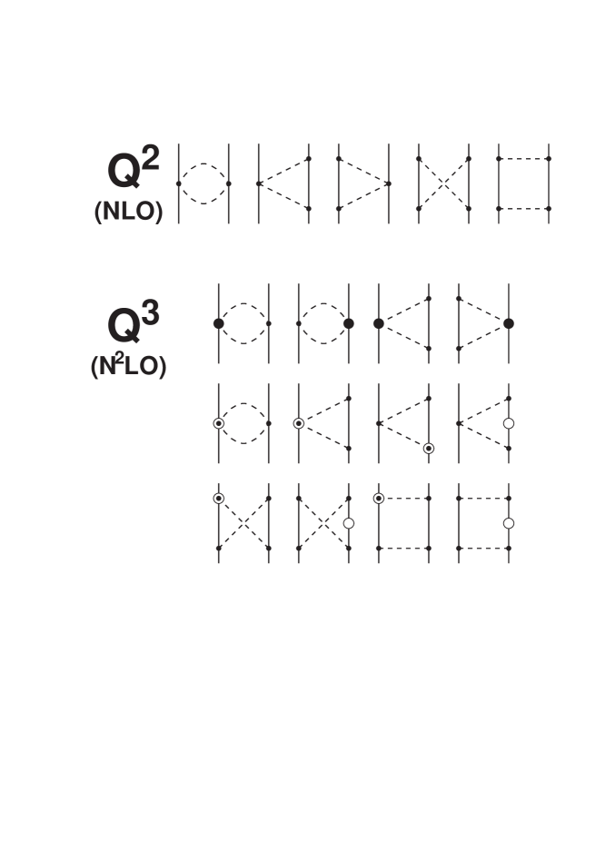
FIG. 1.: Two-pion exchange contributions to the $NN$ interaction at order two and three in small momenta. Solid lines represent nucleons and dashed lines pions. Small dots denote vertices from the leading order $\pi N$ Lagrangian $\widehat{\cal L}^{(1)}_{\pi N}$, Eq. (9). Large solid dots are vertices proportional to the LECs $c_{i}$ from the second order Lagrangian $\widehat{\cal L}^{(2)}_{\pi N,\,\rm ct}$, Eq. (13). Symbols with an open circles are relativistic $1/M_{N}$ corrections contained in the second order Lagrangian $\widehat{\cal L}^{(2)}_{\pi N}$, Eqs. (11). Only a few representative examples of $1/M_{N}$ corrections are shown and not all.

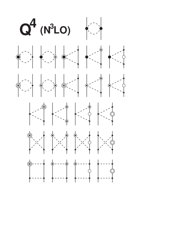
FIG. 2.: One-loop $2\pi$-exchange contributions to the $NN$ interaction at order four. Basic notation as in Fig. 1. Symbols with a large solid dot and an open circle denote $1/M_{N}$ corrections of vertices proportional to $c_{i}$. Symbols with two open circles mark relativistic $1/M^{2}_{N}$ corrections. Both corrections are part of the third order Lagrangian $\widehat{\cal L}^{(3)}_{\pi N}$, Eq. (15). Representative examples for all types of one-loop graphs that occur at this order are shown.

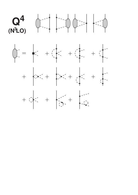
FIG. 3.: Two-loop $2\pi$-exchange contributions at order four. Basic notation as in Fig. 1. The grey disc stands for all one-loop $\pi N$ graphs some of which are shown in the lower part of the figure. The solid square represents vertices proportional to the LECs $d_{i}$ which are introduced by the third order Lagrangian ${\cal L}^{(3)}_{\pi N}$, Eq. (14). More explanations are given in the text.

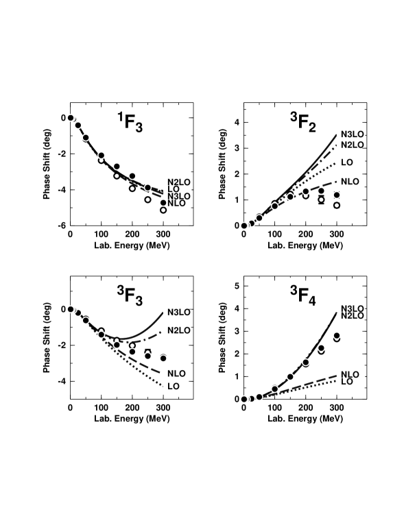
FIG. 4.: $F$-wave phase shifts of neutron-proton scattering for laboratory kinetic energies below 300 MeV. We show the predictions from chiral pion exchange to leading order (LO), next-to-leading order (NLO), next-to-next-to-leading order (N2LO), and next-to-next-to-next-to-leading order (N3LO). The solid dots and open circles are the results from the Nijmegen multi-energy $np$ phase shift analysis [34] and the VPI single-energy $np$ analysis SM99 [35], respectively.

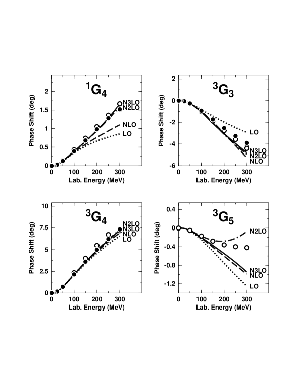
FIG. 5.: Same as Fig. 4, but for $G$-waves.

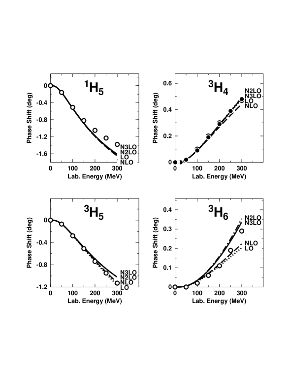
FIG. 6.: Same as Fig. 4, but for $H$-waves.

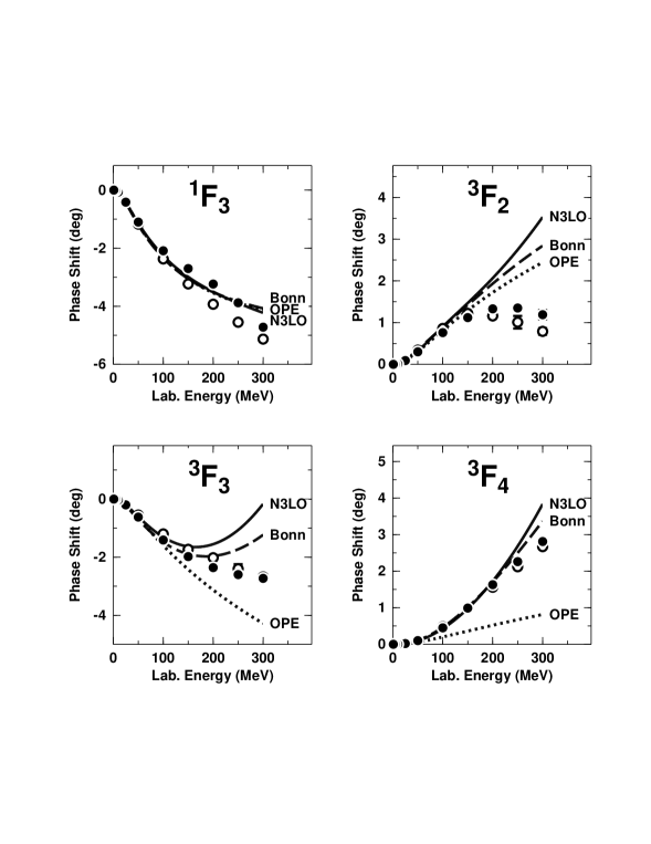
FIG. 7.: $F$-wave phase shifts of neutron-proton scattering for laboratory kinetic energies below 300 MeV. We show the results from one-pion-exchange (OPE), and one- plus two-pion exchange as predicted by $\chi$PT at next-to-next-to-next-to-leading order (N3LO) and by the Bonn Full Model [36] (Bonn). Empirical phase shifts (solid dots and open circles) as in Fig. 4.

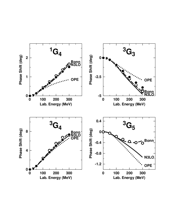
FIG. 8.: Same as Fig. 7, but for $G$-waves.

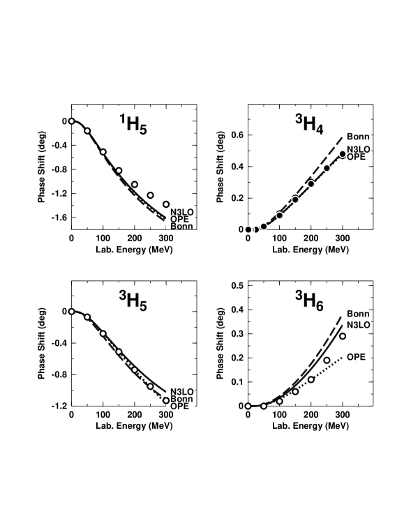
FIG. 9.: Same as Fig. 7, but for $H$-waves.

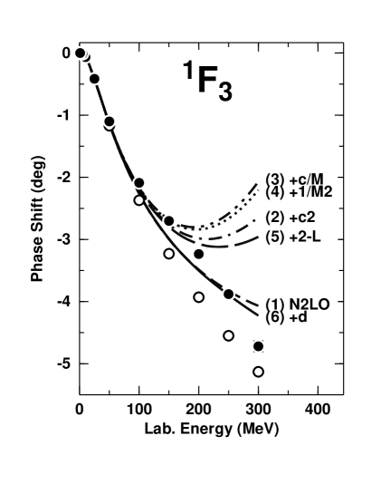
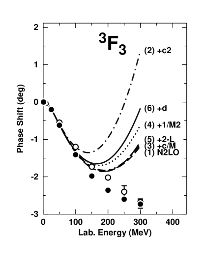
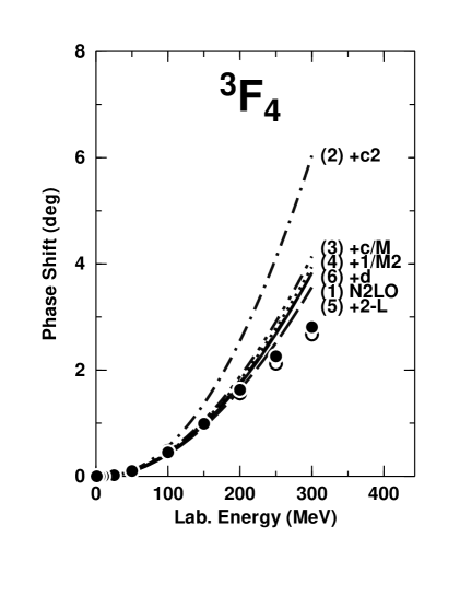
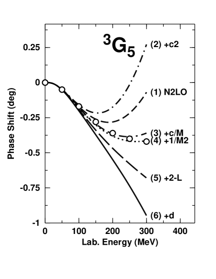
FIG. 10.: The effect of individual order-four contributions on the neutron-proton phase shifts in some selected peripheral partial waves. The individual contributions are added up successively in the order given in parenthesis next to each curve. Curve (1) is N2LO and curve (6) is the complete N3LO. For further explanations, see Appendix A. Empirical phase shifts (solid dots and open circles) as in Fig. 4.

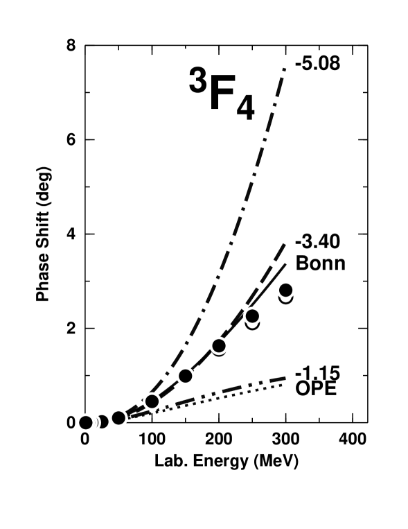
FIG. 11.: One and two-pion exchange contributions at order four to the ${}^{3}F_{4}$ phase shifts for three different choices of the LEC $c_{3}$. The numbers given next to the curves denote the values for $c_{3}$ in units of GeV^-1 used for the respective curves (all other parameters as in Table I). For comparison, we also show the OPE contributrion (OPE) and the result from $\pi$ + $2\pi$ exchange of the Bonn model (Bonn). Empirical phase shifts (solid dots and open circles) as in Fig. 4.

REFERENCES

- [1] S. Weinberg, Phys. Lett. B 251, 288 (1990); Nucl. Phys. B363, 3 (1991).
- [2] C. Ordóñez and U. van Kolck, Phys. Lett. B 291, 459 (1992).
- [3] C. Ordóñez, L. Ray, and U. van Kolck, Phys. Rev. Lett. 72, 1982 (1994); Phys. Rev. C 53, 2086 (1996).
- [4] U. van Kolck, Prog. Part. Nucl. Phys. 43, 337 (1999).
- [5] L. S. Celenza, A. Pantziris, and C. M. Shakin, Phys. Rev. C 46, 2213 (1992).
- [6] C. A. da Rocha and M. R. Robilotta, Phys. Rev. C 49, 1818 (1994); ibid. 52, 531 (1995); M. R. Robilotta, Nucl. Phys. A595, 171 (1995); M. R. Robilotta, and C. A. da Rocha, Nucl. Phys. A615, 391 (1997); J.-L. Ballot, C. A. da Rocha, and M. R. Robilotta, Phys. Rev. C 57, 1574 (1998).
- [7] N. Kaiser, R. Brockmann, and W. Weise, Nucl. Phys. A625, 758 (1997).
- [8] N. Kaiser, S. Gerstendörfer, and W. Weise, Nucl. Phys. A637, 395 (1998).
- [9] N. Kaiser, Phys. Rev. C 61, 014003 (1999); ibid. 62, 024001 (2000).
- [10] N. Kaiser, Phys. Rev. C 63, 044010 (2001).
- [11] N. Kaiser, Phys. Rev. C 64, 057001 (2001).
- [12] N. Kaiser, Phys. Rev. C 65, 017001 (2002).
- [13] E. Epelbaum, W. Glöckle, and U.-G. Meißner, Nucl. Phys. A637, 107 (1998); ibid. A671, 295 (2000).
- [14] D. R. Entem and R. Machleidt, Phys. Lett. B524, 93 (2002).
- [15] D. B. Kaplan, M.J. Savage, and M.B. Wise, Nucl. Phys. B478, 629 (1996); D. B. Kaplan, Nucl. Phys. B494, 471 (1997); D. B. Kaplan, M.J. Savage, and M.B. Wise, Nucl. Phys. B534, 329 (1998); Phys. Lett. B424, 390 (1998).
- [16] R. J. Furnstahl, B. D. Serot, and H.-B. Tang, Nucl. Phys. A615, 441 (1997); J. V. Steel and R. J. Furnstahl, ibid. A637, 46 (1998); R. J. Furnstahl, J. V. Steel, and N. Tirfessa, ibid. A671, 396 (2000); R. J. Furnstahl, H. W. Hammer, and N. Tirfessa, ibid. A689, 846 (2001).
- [17] T.-S. Park, K. Kubodera, D. P. Min, and M. Rho, Phys. Rev. C 58, 637 (1998); Nucl. Phys. A646, 83 (1999).
- [18] T. D. Cohen, Phys. Rev. C 55, 67 (1997); D. R. Phillips and T. D. Cohen, Phys. Lett. B390, 7 (1997); K. A. Scaldeferri, D. R. Phillips, C. W. Kao, and T. D. Cohen, Phys. Rev. C 56, 679 (1997); S. R. Beane, T. D. Cohen, and D. R. Phillips, Nucl. Phys. A632, 445 (1998).
- [19] G. Rupak and N. Shoresh, nucl-th/9906077; P. F. Bedaque, H. W. Hammer, and U. van Kolck, Nucl. Phys. A676, 357 (2000); S. Fleming, Th. Mehen, and I. W. Stewart, Nucl. Phys. A677, 313 (2000); Phys. Rev. C 61, 044005 (2000).
- [20] S. R. Bean, P. F. Bedaque, M. J. Savage, and U. van Kolck, nucl-th/0104030.
- [21] M. C. M. Rentmeester, R. G. E. Timmermans, J. L. Friar, and J. J. de Swart, Phys. Rev. Lett. 82, 4992 (1999).
- [22] N. Fettes, U.-G. Meißner, S. Steiniger, Nucl. Phys. A640, 199 (1998).
- [23] N. Fettes, U.-G. Meißner, M. Mojžiš, and S. Steininger, Ann. Phys. (N.Y.) 283, 273 (2000); ibid. 288, 249 (2001).
- [24] V. Stoks, R. Timmermans, and J. J. de Swart, Phys. Rev. C 47, 512 (1993).
- [25] R. A. Arndt, R. L. Workman, and M. M. Pavan, Phys. Rev. C 49, 2729 (1994).
- [26] Review of Particle Physics, Eur. Phys. J. C 15, 1 (2000).
- [27] P. Büttiker and U.-G. Meißner, Nucl. Phys. A668, 97 (2000).
- [28] V. Bernard, N. Kaiser, and U.-G. Meißner, Int. J. Mod. Phys. E 4, 193 (1995).
- [29] G. Q. Li and R. Machleidt, Phys. Rev. C 58, 3153 (1998).
- [30] M. Jacob and G. C. Wick, Ann. Phys. (N.Y.) 7, 404 (1959).
- [31] J. Goto and S. Machida, Prog. Theor. Phys. 25, 64 (1961).
- [32] K. Erkelenz, R. Alzetta, and K. Holinde, Nucl. Phys. A176, 413 (1971); note that there is an error in equation (4.22) of this paper where it should read: and .
- [33] H. P. Stapp, T. J. Ypsilantis, and N. Metropolis, Phys. Rev. 105, 302 (1957).
- [34] V. G. J. Stoks, R. A. M. Klomp, M. C. M. Rentmeester, and J. J. de Swart, Phys. Rev. C 48, 792 (1993).
- [35] R. A. Arndt, I. I. Strakovsky, and R. L. Workman, SAID, Scattering Analysis Interactive Dial-in computer facility, Virginia Polytechnic Institute and George Washington University, solution SM99 (Summer 1999); for more information see, e. g., R. A. Arndt, I. I. Strakovsky, and R. L. Workman, Phys. Rev. C 50, 2731 (1994).
- [36] R. Machleidt, K. Holinde, and Ch. Elster, Phys. Rep. 149, 1 (1987).
- [37] Note that the Bonn model uses the coupling constant , while for chiral pion exchanges we apply [cf. footnote of Table I]. This is the main reason for the light “discrepancies” between N3LO and Bonn that seem to show up in some of the waves (Fig. 9).
- [38] In fact, preliminary calculations, which take an important class of diagrams of order five into account, indicate that the N4LO contribution may prevailingly be repulsive (N. Kaiser, private communication).
- [39] G. E. Brown and A. D. Jackson, The Nucleon-Nucleon Interaction, (North-Holland, Amsterdam, 1976).
- [40] R. Vinh Mau, in: Mesons in Nuclei, Vol. I, M. Rho and D. H. Wilkinson, eds. (North-Holland, Amsterdam, 1979) p. 151; M. Lacombe, B. Loiseau, J. M. Richard, R. Vinh Mau, J. Côté, P. Pires, and R. de Tourreil, Phys. Rev. C 21, 861 (1980).
- [41] E. Epelbaum, A. Nogga, W. Glöckle, H. Kamada, U.-G. Meißner, and H. Witala, Few-Nucleon Systems with Two-Nucleon Forces from Chiral Effective Field Theory, nucl-th/0201064.
- [42] M. Chemtob, J. W. Durso, and D. O. Riska, Nucl. Phys. B38, 141 (1972); A. D. Jackson, D. O. Riska, and B. Verwest, Nucl. Phys. A249, 397 (1975).
- [43] R. Vinh Mau, J. M. Richard, B. Loiseau, M. Lacombe, and W. M. Cottingham, Phys. Lett. B44, 1 (1973); M. Lacombe, B. Loiseau, J. M. Richard, R. Vinh Mau, P. Pires, and R. de Tourreil, Phys. Rev. D 12, 1495 (1975).
- [44] We note that in the Nijmegen analysis [21] Gev-1 emerges which also differs from what we use and what is obtained in analysis (cf. Table I). However, this difference in has very little impact on peripheral partial waves and does not make possible stronger values for .