Coupled fermion and boson production in a strong background mean-field

Abstract

We derive quantum kinetic equations for fermion and boson production starting from a $\phi^{4}$ Lagrangian with minimal coupling to fermions. Decomposing the scalar field into a mean-field part and fluctuations we obtain spontaneous pair creation driven by a self-interacting strong background field. The produced fermion and boson pairs are self-consistently coupled. Consequently back reactions arise from fermion and boson currents determining the time dependent self-interacting background mean-field. We explore the numerical solution in flux tube geometry for the time evolution of the mean-field as well as for the number- and energy densities for fermions and bosons. We find that after a characteristic time all energy is converted from the background mean-field to particle creation. Applying this general approach to the production of “quarks” and “gluons” a typical time scale for the collapse of the flux tube is $1.5$ fm/c.
Pacs Numbers: 25.75.Dw,12.38.Mh,05.20.Dd,05.60.Gg

I Introduction

An ultra-relativistic heavy ion collision is a very complex process and its theoretical description requires a fundamental understanding of all phases [1]. After the collision of the nuclei, it is expected that a strongly coupled quark gluon plasma is formed [2]. The production of hard partons due to collisions is one successful way to describe properties of the pre-equilibrium phase [3, 4, 5, 6, 7]. Alternatively the flux-tube model was developed describing the spontaneous creation of soft particles in a chromo-electric background field [8, 9, 10].

The idea is based on the QED picture of spontaneous vacuum pair creation in a strong field [11, 12]. The strong electric background field leads to a restructuring of the Dirac sea and drives the system into a false, unstable vacuum which decays by emitting particles. Experimentally this was never measured because of the insufficiently small fields compared to the mass of the electrons in e.g. optical laser experiments. Planned new facilities such as the X-ray free electron laser (XFEL) may be able to probe the domain of non-perturbative QED and melt the vacuum [13, 14].

In QCD the string tension is large compared to the mass of the partons. Therefore the main application of the Schwinger mechanism is for ultra-relativistic heavy ion collisions to study the production of a strongly coupled system of partons within the flux tube model [8]. Different versions of a Schwinger-like source term have been suggested, e.g. [15, 16, 17], and are implemented in transport equations to describe formation and evolution of a quark-gluon plasma on a phenomenological level.

However the precise connection between field theoretical approaches and a kinetic theory is very challenging and an unsolved problem in general. For the considered example of the Dirac/Klein-Gordon equation in an external field this connection was found in [18, 19]. The resulting quantum Vlasov equation was successfully applied to fermion- and boson pair creation [19, 20, 21].

In the applications considered so far either fermions or bosons were treated. One important aspect of most of the studies was the appearance of plasma oscillations due to back reactions [16, 22] and their damping due to collisions [20, 23]. Herein we introduce a self-consistent scheme in which fermion and boson fields are coupled via a strong background mean field. This internal field replaces the external field description of recent approaches and dynamically couples fermion and boson production. This coupling is most important for the back reactions since the total induced current consists of both fermionic and bosonic contributions. We solve the resulting coupled equations in cylinder geometry [24] to implement physical boundary conditions leading to a lower bound in the infra-red momentum region. This procedure not only satisfies the geometry constraints characteristic for a flux tube but also allows the production of massless scalar particles (“gluons”). The fermionic “quark” mass is treated as a momentum and temperature dependent quantity as obtained from QCD Dyson-Schwinger equation investigations [17, 25].

The article is organized as follows. In Section II we introduce the effective Lagrangian which we use to derive the kinetic equations. In Section III we introduce cylindric boundary conditions for which we solve the equations numerically in Section IV. We summarize our results in Section V.

II Effective Lagrangian and equation of motions

In this article we will adopt the flux tube picture. One important aspect is the particular geometry assuming that the “chromo-electric” field acts along the longitudinal direction. We introduce the arbitrary fixed 4-vector $n_{\mu}$ which allows the implementation of the flux tube geometry as described below.

We start our discussion from the following Lagrangian for fermions and bosons:

$$L(x) = \partial_{\mu}\Phi^{*}(x)\partial^{\mu}\Phi(x)-m_{+}^{2}\left|{\Phi(x)}\right|^{2}-e_{+}^{2}\left|{\Phi(x)}\right|^{4}$$ (4)

$$+ie_{+}\left\{{[\nabla_{n}\Phi^{*}(x)]\Phi^{2}(x)-[\Phi^{*}(x)]^{2}\nabla_{n}\Phi(x)}\right\}$$

$$+\frac{i}{2}\overline{\psi}(x)\gamma^{\mu}\stackrel{{\scriptstyle\leftrightarrow}}{{\partial}}_{\mu}\psi(x)-m_{-}\overline{\psi}(x)\psi(x)$$

$$-\frac{e_{-}}{2}\left(\Phi(x)+\Phi^{*}(x)\right)\overline{\psi}(x)(\gamma n)\psi(x)\,\,,$$

where (-) denotes fermions, $\psi$, and (+) bosons, $\Phi$. The operator $\nabla_{n}=n^{\mu}\partial_{\mu}$ permits to introduce the self-interacting scalar field with first order derivative only. The total field, $\Phi(x)$, can be decomposed into a mean field contribution, $\Phi_{0}$, and fluctuations around it, $\varphi$, (e.g. [26])

$$\Phi(x)=\Phi_{0}(t)+\varphi(x)\,.$$ (5)

We consider $\Phi_{0}(t)$ as a neutral, space-homogeneous background mean field: $\Phi_{0}=<\Phi>$. The field of the fluctuations $\varphi(x)$ is in general complex corresponding to a charged field with a vanishing mean value $<\varphi(x)>=0$. The Lagrangian (4) contains in particular terms of the order $|\Phi(x)|^{4}$ related to self-interaction. As we will discuss below, we keep the $|\Phi(x)|^{4}$ contribution to determine only the background field $\Phi_{0}(t)$. That makes possible a proper inclusion of back reactions. However we neglect all higher orders in the fluctuations in deriving the equations of motion and the kinetic equations. That means we restrict ourselves to the limit without collisions. We obtain the following Lagrangian for the quantum fluctuations in mean field approximation

$$L^{-}(x) = \frac{i}{2}\overline{\psi}(x)\gamma^{\mu}\stackrel{{\scriptstyle\leftrightarrow}}{{\partial}}_{\mu}\psi(x)-m_{-}\overline{\psi}(x)\psi(x)$$ (7)

$$+e_{-}\Phi_{0}(t)\overline{\psi}(x)(n_{\mu}\gamma^{\mu})\psi(x)\,,$$

$$L^{+}(x) = \partial_{\mu}\varphi^{*}(x)\partial^{\mu}\varphi(x)-m_{+}^{2}\left|{\varphi(x)}\right|^{2}$$ (10)

$$+ie_{+}\Phi_{0}(t)\left[{(\nabla_{n}\varphi^{*}(x))\varphi(x)-\varphi^{*}(x)\nabla_{n}\varphi(x)}\right]$$

$$-e_{+}^{2}|\Phi_{0}(t)|^{2}\left|{\varphi(x)}\right|^{2}\,.$$

The corresponding equations of motion are found within standard techniques and read

$$\bigg{(}i\gamma^{\mu}\partial_{\mu}-e_{-}\gamma^{\mu}n_{\mu}\Phi^{0}(t)-m_{-}\bigg{)}\psi(x) = 0\,,$$ (11)

$$\left[D^{*}_{\mu}D^{\mu}+m_{+}^{2}\right]\varphi(x) = 0\,,$$ (12)

$$\partial_{0}^{2}\Phi_{0}(t)+m_{+}^{2}\Phi_{0}(t)+4e_{+}^{2}\Phi_{0}^{3}(t)-j_{-}-j_{+} = 0\,,$$ (13)

where Eq. (11) is the Dirac equation, Eq. (12) is the Klein-Gordon equation with the covariant derivative

$$D_{\mu}=\partial_{\mu}+ie_{+}n_{\mu}\Phi_{0}(t)$$ (14)

and Eq. (13) provides the time dependent background mean field. It is important to observe that the external gauge field which typically appears in applications for pair creation in strong fields in the Dirac and Klein-Gordon equation is replaced by an internal mean field $\Phi_{0}$. The third term on the left-hand side of Eq. (13) is non-linear and appears as result of the $|\Phi|^{4}$ self-interacting contribution in the Lagrangian (4). The second (mass term) and the third term are not contained in the external field description. The equations of motion are self-consistently coupled, i.e. the mean background field acts on the fluctuations and vice versa: the produced charged particles generate the currents forming the background field. That is the well-know back reaction phenomenon. The contraction of these currents with $n^{\mu}$ reads

$$j_{-}(t) = -e_{-}<\overline{\psi}(x)(\gamma n)\psi(x)>,$$ (15)

$$j_{+}(t) = -e_{+}<i\varphi^{*}(x)\nabla_{n}\varphi(x)-i(\nabla_{n}\varphi^{*}(x))\varphi(x)$$ (17)

$$-2e_{+}\Phi_{0}(t)\varphi^{*}(x)\varphi(x)>\,.$$

In the following we will identify the fermions as “quarks” and the bosons as “gluons”, i.e. we consider the “gluons” to be scalar. Alternatively one could consider the bosons as a vector field and such an approach is demonstrated in the Appendix A yielding the same Lagrangian as Eq. (10). Many aspects of QCD are not contained in our approach and clearly to identify the fermionic and bosonic degrees of freedom with “quarks and gluons” is a very optimistic view. However we hope that some qualitative features discussed below are robust and also hold for more sophisticated theories than our toy model.

One way to proceed is to solve the equations of motions directly. We are interested in finding kinetic equations being the exact analogue to these equations of motion. Starting from Eqs. (11) and (12) it is possible to derive such quantum kinetic equations. In [18, 19] it was explained in detail how to introduce quasi-particles, diagonalize the interaction Hamiltonian and describe the transition from an unstable to a stable vacuum as a dynamical process employing a time-dependent Bogolyubov transformation. The resulting equation for the single particle distribution function is exact on the mean field level in a space-homogeneous field, i.e. it preserves the quantum statistical nature and the pair creation phenomenon. We choose $n_{\mu}=(0,0,0,1)$ which is equivalent to considering a vector potential in temporal gauge with a background field acting in z-direction. We obtain

$$\frac{{\partial f_{\pm}({\bar{p}},t)}}{{\partial t}}+e_{\pm}\sigma(t)\frac{{\partial f_{\pm}({\bar{p}},t)}}{{\partial p_{\parallel}}}=S_{\pm}({\bar{p}},t),$$ (18)

where $\sigma(t)=-d\Phi_{0}(t)/dt$ is the space-homogeneous time dependent “chromo-electric” field strength, $f_{\pm}({\bar{p}},t)$ is the distribution function of the partons in quasi-particle approximation and $S_{\pm}({\bar{p}},t)$ is the source term

$$S_{\pm}({\bar{p}},t) = \frac{1}{2}W_{\pm}({\bar{p}},t)\int\limits_{-\infty}^{t}{dt^{\prime}}W_{\pm}({\bar{p}},t,t^{\prime})\times$$ (20)

$$\left[1\pm 2f_{\pm}(P_{\pm}(t,t^{\prime}),t^{\prime})\right]\cos\left\{{2\int\limits_{t^{\prime}}^{t}{d\tau}\omega_{\pm}({\bar{p}};t,\tau)}\right\}$$

describing the creation and annihilation processes of fermions and bosons as result of vacuum tunneling in a strong quasi-classical mean-field $\Phi_{0}(t)$. The transition amplitudes are

$$W_{\pm}({\bar{p}};t,t^{\prime})=\frac{{e_{\pm}\sigma(t^{\prime})P_{\pm}(t,t^{\prime})}}{{\omega_{\pm}^{2}({\bar{p}};t,t^{\prime})}}\left[{\frac{\varepsilon_{\pm\perp}}{{P_{\pm}(t,t^{\prime})}}}\right]^{2s_{\pm}}\,.$$ (21)

For fermions $s_{-}=1/2$ and for bosons $s_{+}=0$. The energy squared of the quasi-particles reads

$$\omega^{2}_{\pm}({\bar{p}},t,t^{\prime}) = \varepsilon_{\pm\perp}^{2}+P_{\pm}^{2}(t,t^{\prime})\,,$$ (22)

$$P_{\pm}(t,t^{\prime}) = p_{\parallel}-e_{\pm}\int\limits_{t^{\prime}}^{t}{d\tau\sigma(\tau)}\,,$$ (23)

where $\varepsilon^{2}_{\pm\perp}=m_{\pm}^{2}+p_{1}^{2}+p_{2}^{2}$ is the transverse energy. It is assumed that $\mathop{\lim}\limits_{t\to-\infty}\sigma(t)=0$ and we simplify the notation by introducing

$$\omega_{\pm}({\bar{p}})=\omega_{\pm}({\bar{p}},t,t)\,\,,\qquad W_{\pm}({\bar{p}},t)=W_{\pm}({\bar{p}},t,t)\,.$$ (24)

The kinetic equations (18) coincide with recent results and retain all physical information contained in the field equations (11)-(12). The main properties of the source term are the inclusion of quantum statistical effects due to the Fermi suppression (Bose enhancement) factor for fermions (bosons) and the nonlocal time structure. “Quarks and gluons” are produced with a non-trivial, non-equilibrium momentum distribution which is different in transverse- and in longitudinal direction to which the field $\Phi_{0}$ couples according to the chosen anisotropy. Apart from the conceptual interest of a kinetic formulation, the practical merits are obvious: e.g. the straightforward identification of the Markovian- or low density limit and the phenomenologically simple inclusion of collisions.

The background field $\Phi_{0}$ decays through particle creation and generation of currents which are readily obtained:

$$j_{\pm}(t)=2\,e_{\pm}g_{\pm}\int\,\frac{d^{3}p}{(2\,\pi)^{3}}\bigg{(}\frac{p_{\parallel}}{\omega_{\pm}({\bar{p}})}f_{\pm}({\bar{p}},t)+$$ (25)

$$\frac{\omega_{\pm}({\bar{p}})}{e_{\pm}\sigma(t)}\frac{df_{\pm}({\bar{p}},t)}{dt}-\frac{e_{\pm}\dot{\sigma}(t)p_{\parallel}}{8\omega^{4}_{\pm}({\bar{p}})}\bigg{[}\frac{\epsilon_{\bot\pm}}{p_{\parallel}}\bigg{]}^{2s_{\pm}}\bigg{)}\,,$$ (26)

where $g_{\pm}$ is the degeneracy factor The first term is proportional to the occupation number itself and the second term is related to polarization being proportional to the rate. The last term is a regularizing counter term. Its origin is associated with charge regularization; further details can be found in [16].

III Cylindric boundary and the flux tube geometry

Another element that we would like to introduce in our model is a cylindrically confined region for the particle production process. A similar approach was explored in [24, 29] and an advanced description of a dynamical flux tube was given in [30]. The background field is constructed to act only inside a cylindric tube and is assumed to vanish outside this finite volume. We introduce this feature because of two reasons: (i) to implement the given anisotropic symmetry and (ii) to avoid difficulties with massless particle production for “gluons”. It is clear that a finite size in transverse direction leads to a quantization of the transverse momentum, so that at zero mass $m_{+}=0$ the minimal energy at which particles can be produced is $\Lambda^{IR}$.

One possible, simple way is to introduce the boundary conditions

$$\Phi(x_{3},\rho_{0},\phi,t)=0$$ (27)

to require that the field vanishes outside a fixed flux tube of the radius $\rho_{0}$, e.g. [24]. The Klein-Gordon equation in such cylinder coordinates reads

$$\bigg{[}\partial_{0}^{2}-\nabla_{\perp}^{2}-\partial_{3}^{2} - 2ie_{+}\Phi_{0}(t)\partial_{3}-e_{+}^{2}\Phi_{0}^{2}(t)$$ (28)

$$+ m_{+}^{2}\bigg{]}\varphi(x_{3},\rho,\phi,t)=0,$$ (29)

where the Laplace operator is given by

$$\nabla^{2}_{\perp}=\frac{\partial^{2}}{\partial\rho^{2}}+\frac{1}{\rho}\frac{\partial}{\partial\rho}+\frac{1}{\rho^{2}}\frac{\partial^{2}}{\partial\phi^{2}}\,.$$ (30)

The radius is denoted with $\rho$ and the angle is $\phi$. Here we assume that the mean field depends only on time and not explicitly on the radius: $\Phi_{0}=\Phi_{0}(t)$. This assumption allows to make a separable ansatz of the following form

$$\varphi(x_{3},\rho,\phi,t)=Ne^{il\phi}e^{-ik_{3}x_{3}}T(t)R(\rho)\,.$$ (31)

Substituting (31) into (28) we find two equations, one for the time dependent part

$$\ddot{T}(t)+\left[m_{+}^{2}+\left(k_{3}-e_{+}\Phi_{0}(t)\right)^{2}+\varepsilon^{2}\right]T(t)=0$$ (32)

and one for the spatial dependence

$$\rho^{2}R^{{}^{\prime\prime}}(\rho)+\rho R^{{}^{\prime}}(\rho)+\left(\varepsilon^{2}\rho^{2}-l^{2}\right)R(\rho)=0\,,$$ (33)

where $\varepsilon$ is any constant value. The latter equation is known as the Bessel equation and with the boundary condition $R(\varepsilon\rho_{0})=0$. Eq. (31) can be rewritten in terms of Bessel functions

$$\varphi_{nl,k_{3}}(x_{3},\rho,\phi,t)=e^{-ik_{3}x_{3}}T_{nl}(t)\frac{J_{l}(\varepsilon_{nl}\rho)}{\sqrt{\pi}\rho_{0}J^{{}^{\prime}}_{l}(\varepsilon_{nl}\rho_{0})}e^{il\phi},$$ (34)

where $\varepsilon_{nl}\rho_{0}$ is the $n-th$ zero of the Bessel function $J_{l}$.

$\rho_{0}$	1 fm	2 fm	3 fm
$\Lambda^{IR}$	0.48 GeV	0.24 GeV	0.16 GeV

TABLE I.: The radius of the flux tube $\rho_{0}$ is fixed and leads to a discretized momentum with a lower bound $\Lambda^{IR}$.

The resulting kinetic equations are identical to Eqs. (18) but the quasi-particle energy is now discrete and reads

$$\omega_{\pm nl}^{2}({\bar{p}},t) = \varepsilon_{+\bot nl}^{2}+(k_{3}-e_{\pm}\Phi_{0}(t))^{2}\,,$$ (35)

$$\varepsilon^{2}_{\pm\bot nl} = m_{\pm}^{2}+\varepsilon^{2}_{nl}\,.$$ (36)

The kinetic momentum $p_{\parallel}=k_{3}-e_{\pm}\Phi_{0}(t)$ contains the time dependent mean-field and the canonical momentum $k_{3}$. The lowest possible values for the transverse energy are assumed for $\varepsilon_{10}$ and the corresponding $\Lambda^{IR}=\varepsilon_{10}$ are given in Table I for three different flux tube radii. This means that the transverse energy never vanishes. Even for a zero gluon mass the discretization provides a lower bound for the momentum. To proceed we consider all observable values as mean values in the following way

$$<<...>>_{\rho}=\frac{1}{\pi\rho_{0}^{2}}\int_{0}^{\rho_{0}}\rho d\rho\int_{0}^{2\pi}d\phi<...>\,.$$ (37)

Assuming such mean ($\rho$- independent) quantities is a very simple approximation. However for the qualitative study performed it is sufficient and can certainly be improved for a particular experimental application. The charges in strong coupling limit are fixed to be $e_{\pm}=1$ throughout the numerical calculations and the degeneracy factors for a three flavor system are for quarks $g_{-}=18$ and for gluons $g_{+}=16$. Quantitatively the numerical results depend on these values, qualitatively the main effects discussed below are robust against small changes of all parameter values.

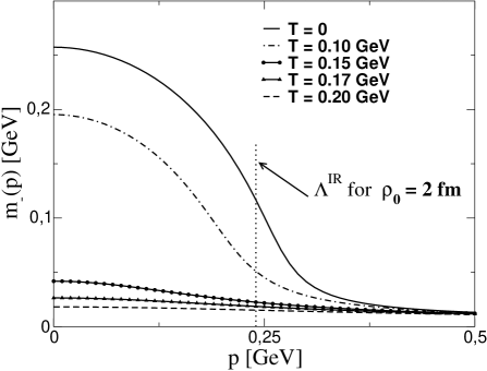
FIG. 1.: Momentum dependence of the quark mass for different temperatures obtained from solving the QCD Dyson-Schwinger equation for the quarks employing a simplified gluon propagator. The fixed radius of the flux tube, $\rho=2$ fm, leads to a lower momentum bound of $\Lambda^{IR}=0.24$ GeV.

Before we present our numerical results we briefly discuss the mass scales of the produced particles. The “gluon” mass is chosen to be zero or finite. This is possible because of the geometry constraint discussed above. The fermion mass is very small on the hadronic scale in the perturbative regime, $m_{-}(p\rightarrow\infty)<<\Lambda_{QCD}$. In the non-perturbative domain dynamical chiral symmetry breaking appears and the quark mass increases by about two orders of magnitude $m_{-}(p\rightarrow 0)\sim\Lambda_{QCD}$. For very large temperatures the quarks can be well approximated by their current quark mass for all momenta. However in vicinity of the phase transition a dynamical mass is generated. Furthermore, non-perturbative effects are manifest up to $2-3\times T_{c}\sim 300-450$ MeV. It was shown in a variety of model approaches that within the parton creation model employed in our investigation such temperatures are initially reached. Due to a rapid expansion the temperature will further decrease and non-perturbative dressing of the quarks appears.

In QCD the momentum dependence of the quark mass can be calculated on the lattice, e.g. in [31] in Landau gauge. QCD Dyson-Schwinger equation models [17, 25, 32] are in good agreement with these studies and we employ a simple model introduced in [33] extended to non-zero temperature and density in [17, 34]. The instantaneous version of such an infrared dominant model [17, 35] leads to the following QCD gap equation for the scalar part of the self-energy:

$$b({\bar{p}}) = m_{0}+\eta\frac{m_{-}({\bar{p}})}{\sqrt{{\bar{p}}^{2}+m_{-}^{2}({\bar{p}})}}\times$$ (39)

$$[1-f^{eq}_{-}({\bar{p}},T,\mu)-{\bar{f}}^{eq}_{-}({\bar{p}},T,\mu)]$$

and the vector part

$$a({\bar{p}})=\frac{2b({\bar{p}})}{m_{0}+b({\bar{p}})}$$ (40)

where $m_{-}=b/a$. $f^{eq}_{-}$ and ${\bar{f}}^{eq}_{-}$ are the Fermi distribution functions for particles and antiparticles, respectively. The value of the mass scale parameter $\eta=1$ GeV is inspired by the potential energy in a QCD string at the confinement distance, $V_{q{\bar{q}}}(r=1{\rm fm})\sim 1$ GeV. The momentum dependence calculated with Eq. (39) is depicted in Fig. 1 for different temperatures. The chemical potential is $\mu=0$ and the current quark mass $m_{0}=5$ MeV. For further calculations we will use the shape corresponding to $T=T_{c}\sim 170$ MeV. For the current application a constant fermion mass with the value of $m_{0}$ would provide a good guide. However for future applications, it will be very useful to have its complete temperature and momentum dependence introduced already.

IV Numerical results

The final equations solved numerically are given in the Appendix B. In the following we compare the model cases (i) coupled fermion and boson production with non-linear self-interaction included; (ii) only boson production with self-interaction, i.e neglecting the fermionic contribution, $j_{-}$ in Eq. (13) to (iii) boson production without self-interaction, i.e. neglecting the nonlinear term in Eq. (13) and $j_{-}$ . Furthermore we will explore the dependence of the numerical results on the parameters of the model, i.e. the masses and the flux tube radius, see Table I. We use (a) a zero “gluonic” mass $m_{+}=0$ and compare the results with (b) a finite “gluon” mass of $m_{+}=0.5$ GeV; the mass of the quarks is given by the simple model defined by Eq. (39).

A The mean background field

We start the discussion of the numerical results with the background mean field $\sigma(t)$. As initial condition for the field we choose $e_{+}\sigma(t=0)=4$ GeV² corresponding to a large initial energy density of about $\epsilon(t=0)\sim 700$ GeV/fm³ related to future LHC experiments. The time dependence of the “chromo-electric” field strength $\sigma(t)$ is plotted Fig. 2.

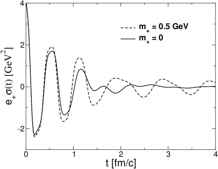
FIG. 2.: The time dependence of the strong background “chromo-electric” field, $\sigma(t)$, for “quarks and gluons” with self-interaction. The flux tube radius is $\rho_{0}=2$ fm and the solutions for two different “gluon” masses $m_{+}=0$ and $m_{+}=0.5$ GeV are compared . For zero “gluon” mass the flux tube collapses at $\tau_{f}\sim 1.5-2$ fm/c and all energy is transformed from the mean field to the created particles. For massive “gluons” weak plasma oscillations survive.

The self-interaction leads to oscillations on a time scale of $\tau_{pl}\sim 0.5$ fm/c in the early phase of the evolution. This result is basically independent of the masses used, however it strongly depends on the initial field strength. The amplitude of the oscillations is damped due to back reactions and the background mean-field vanishes after a few periods at about $\tau_{f}\sim 3\tau_{pl}\sim 1.5$ fm/c for the case of zero gluonic mass. With other words: the field leading to pair creation disappears, the flux tube dynamically collapses. For $m_{+}=0.5$ GeV the oscillations at the beginning of the evolution are damped as well but at $\tau_{f}$ the field does not disappear completely. It rather evolves into a permanently oscillating field with an amplitude of 10% of the initial value. This behavior for $t>\tau_{f}$ can be compared to typical results in an external field approach where a constant background field or an impulse shape was applied and undamped plasma oscillations appeared. The production of quarks is much less effected, see Fig 3, and a physical explanation of this effect seems to be straightforward:

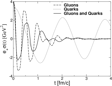
FIG. 3.: The time dependence of the strong background “chromo-electric” field, $\sigma(t)$, for a flux tube radius of $\rho_{0}=2$ fm for “quarks and gluons” with self-interaction (solid line), “gluons” only with self-interaction (dashed line) and “quarks” only (dotted line). The “quarks” are much less effected by the dynamical coupling compared to the “gluons”, cf. Fig. 4. Inclusion of the “quarks” leads to a faster damping of the oscillations in the beginning of the evolution.

The field energy is transformed into the energy of the produced partons, i.e. the amplitude of the oscillations for $t<\tau_{f}$ is decreasing with time. In the vicinity of large magnitudes of $\sigma(t)$ the current is zero since the partons stop their collective motion within the flux tube and at this time the distribution function is symmetrically peaked around zero momentum [20]. For fermions Pauli blocking is most efficient and no particles can be produced in already occupied states. For bosons, however, the enhancement of particle production has its maximum at this time and a large number of bosons is produced. Therefore a direct flow of energy from the field to the gluons occurs, i.e. the damping of the mean field happens very sufficiently. With other words, the quantum statistical nature leads to a fast energy transformation for bosons but to a suppressed one for fermions.

The origin of the collapse of the flux tube is the back reaction phenomenon [36], the time scale on which this appears is given by self-interaction, see Fig. 4. This becomes clear by neglecting the non-linear terms in Eq. (13). That is one new result of the present investigation. The plasma oscillations are smoothly damped only, i.e. the energy is slowly converted from the mean field to the produced particles. In that case the background vanishes at much larger times.

There is only a weak dependence of the results for the mean-field on the flux tube radius. Using the different radii given in Table I, the time scale $\tau_{f}$ is changed by about 10 % but all qualitative effects are unchanged. For values of $\Lambda^{IR}\sim m_{+}$, the lower bound in momentum acts like a mass scale itself and leads to similar results as discussed above in connection with the finite gluon mass. Numerical examples of that consideration are given in the next subsection.

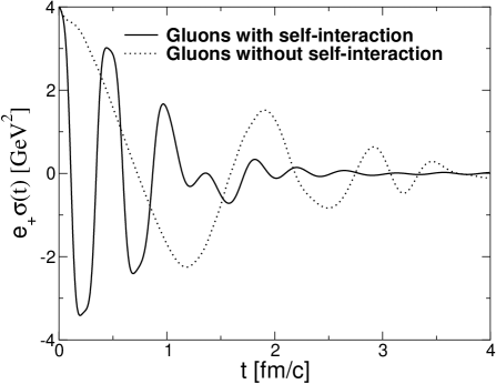
FIG. 4.: The time dependence of the strong background “chromo-electric” field, $\sigma(t)$, for “gluons” with (solid line) and without (dotted line) self-interaction. The flux tube radius is $\rho_{0}=2$ fm and $m_{+}=0$. It is apparent that the inclusion of self-interaction leads to a rapid collapse of the mean background field. Without self-interaction the energy is smoothly converted from the field to the particles.

B Particle production

The self-consistent solution of the quantum kinetic equations for quarks and gluons provides particle creation and a strong background mean-field discussed in the previous section. The large strength of the field initiates the particle production process and “quark”- and “gluon” pairs are spontaneously produced. In Fig. 5 we plot the number density

$$n_{\pm}(t)=\frac{g_{\pm}}{\pi\rho_{0}^{2}}\sum_{nl}\int\frac{dp_{\parallel}}{2\pi}\,\,f_{\pm}(\vec{p},t)$$ (41)

of the produced “quarks and gluons”. It is simple to verify that Eq. (41) is a finite expression, e.g. by using the equations given in Appendix B. At the beginning of the evolution the background field is very large and therefore many particles are produced in a short time. At the same time the background field decreases, energy is converted from the field into the created particles. At $\tau_{f}\sim 1.5$ fm/c the background mean-field vanishes and consequently no more quarks and gluons are produced and the number density assumes a constant value. The number density is very large and therefore it is necessary to solve the full non-Markovian equation (18). The application of the low density limit would underestimate the production of “gluons” and overestimate the “quark” production. Note that, in a realistic description of the further evolution of the produced plasma, collisions between the partons could equilibrate the system. Additionally, the number density would decrease when an expansion is implemented.

The regularized energy density is defined by

$$\epsilon_{\pm}(t)=\frac{g_{\pm}}{\pi\rho_{0}^{2}}\sum_{nl}\int\frac{dp_{\parallel}}{2\pi}\omega_{\pm}(\vec{p})\,\,(f_{\pm}(\bar{p},t)-f_{\pm}^{c}(\bar{p},t))$$ (42)

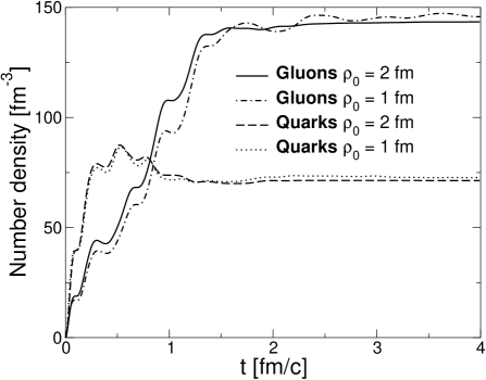
FIG. 5.: The time dependence of the number density for “quarks and gluons”. A fast increase of the particle number is observed at the beginning of the evolution. At $\tau_{f}\sim 1.5$ fm/c the background mean-field vanishes and therefore the creation process stops and the number density is constant. Different flux tube radii do not alter the results significantly.

with the counter term [16, 20]

$$f_{\pm}^{c}(\bar{p},t)=\bigg{[}\frac{e_{\pm}\sigma(t)p_{\parallel}}{4\omega^{3}_{\pm}(\bar{p})}\bigg{(}\frac{\varepsilon_{\pm\perp}}{p_{\parallel}}\bigg{)}^{2s_{\pm}}\bigg{]}^{2}\,.$$ (43)

The time dependence of the energy density is plotted in Fig. 6. Due to the strong background mean-field many particles are produced at small times and energy is converted from the field to the particles (see Fig. 2). During the fast increase of the energy density a shoulder-like structure appears. The period of these waves is in tune with the oscillations of the mean field. The energy density reached at large times for “gluons” is larger compared to the “quarks” due to Pauli blocking acting on the quarks. The value of about $200$ GeV/fm³ corresponds to a (quasi-equilibrium) temperature of about $1$ GeV and is characteristic for planned ultra-relativistic heavy-ion collision experiments. The insertion in Fig. 6 shows the sensitivity to the “gluon” mass. A finite gluon mass leads to weak plasma oscillations in the background mean-field even for large times as discussed in connection with Fig. 2 and therefore the energy density oscillates in concert with these repeated creation and annihilation processes.

Naturally the question arises whether the system is in equilibrium after the production of particles has stopped and no fields are imposed. Although the number- and energy density is constant for large times, the system is still in a strong non-equilibrium state. Further interactions such as inter-parton collisions could provide thermalization, but that is a challenging theoretical question on its own. Further understanding can be provided by studying the pressure for the “quarks and gluons” given by the following expressions:

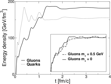
FIG. 6.: The time dependence of the energy density for “quarks and gluons” for $\rho_{0}=2$ fm. Due to the collapse of the background mean field, all energy is converted at $\tau_{f}\sim 1.5$ fm/c into the partons and a constant value of the energy densities is assumed. Different “gluon” masses do not alter the results significantly, see insertion.

$$P_{+}^{\parallel}(t) = \frac{g_{+}}{\pi\rho_{0}^{2}}\sum_{nl}\int\frac{dp_{\parallel}}{2\pi}\bigg{[}\frac{p_{\parallel}^{2}}{\omega_{+}(\vec{p})}\bigg{(}f_{+}(\bar{p},t)-f^{c}_{+}(\vec{p},t)\bigg{)}$$ (45)

$$+\bigg{(}\frac{p_{\parallel}^{2}}{2\omega_{+}(\bar{p})}-\frac{\omega_{+}(\vec{p})}{6}\bigg{)}\bigg{(}v_{+}(\bar{p},t)-v^{c}_{+}(\vec{p},t)\bigg{)}\bigg{]},$$

$$P_{+}^{\perp}(t) = \frac{g_{+}}{2\pi\rho_{0}^{2}}\sum_{nl}\int\frac{dp_{\parallel}}{2\pi}\bigg{[}\frac{(\varepsilon^{+}_{nl})^{2}}{\omega_{+}(\vec{p})}\bigg{(}f_{+}(\bar{p},t)-f^{c}_{+}(\vec{p},t)\bigg{)}$$ (47)

$$+\bigg{(}\frac{(\varepsilon^{+}_{nl})^{2}}{2\omega_{+}(\bar{p})}-\frac{\omega_{+}(\vec{p})}{3}\bigg{)}\bigg{(}v_{+}(\bar{p},t)-v^{c}_{+}(\vec{p},t)\bigg{)}\bigg{]},$$

$$P_{-}^{\parallel}(t) = \frac{g_{-}}{\pi\rho_{0}^{2}}\sum_{nl}\int\frac{dp_{\parallel}}{2\pi}\bigg{[}\frac{p_{\parallel}^{2}}{\omega_{-}(\bar{p})}\bigg{(}f_{-}(\bar{p},t)-f^{c}_{-}(\bar{p},t)\bigg{)}$$ (49)

$$+\frac{\varepsilon^{-}_{\perp}p_{\parallel}}{2\omega_{-}}\bigg{(}v_{-}(\bar{p},t)-v^{c}_{-}(\vec{p},t)\bigg{)}\bigg{]},$$

$$P_{-}^{\perp}(t) = \frac{g_{-}}{2\pi\rho_{0}^{2}}\sum_{nl}\int\frac{dp_{\parallel}}{2\pi}\bigg{[}\frac{(\varepsilon^{-}_{nl})^{2}}{\omega_{-}(\bar{p})}\bigg{(}f_{-}(\bar{p},t)-f^{c}_{-}(\bar{p},t)\bigg{)}$$ (51)

$$-\frac{(\varepsilon^{-}_{nl})^{2}p_{\parallel}}{2\omega_{-}(\bar{p})\varepsilon_{\perp}}\bigg{(}v_{-}(\bar{p},t)-v^{c}_{-}(\vec{p},t)\bigg{)}\bigg{]},$$

where the regularizing counter term $f^{c}$ is given in Eq. (43) and $v^{c}$ reads

$$v_{\pm}^{c}(\bar{p},t)=\frac{e_{\pm}\dot{\sigma}(t)p_{\parallel}}{8\omega^{4}_{\pm}(\bar{p})}\bigg{(}\frac{\varepsilon_{\pm\perp}}{p_{\parallel}}\bigg{)}^{2s_{\pm}}\,.$$ (52)

In Fig. 7 we plot the different components of the pressure. It is apparent that the considered system is still out-off equilibrium. It is interesting to observe that the difference is much more pronounced for “gluons” (lower panel) compared to “quarks” (upper panel). The “gluon” production is unhindered and preferable in longitudinal direction, for “quarks” again Pauli blocking prevents a drastic difference. In an equilibrated system the longitudinal and the parallel pressure contributions would be equal.

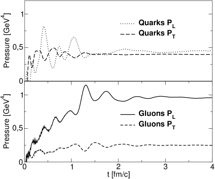
FIG. 7.: The time dependence of the pressure of “gluons” (lower panel) and “quarks” (upper panel). The difference between the longitudinal and transverse part indicates that the system is out-off equilibrium also at large times. Pauli blocking prevents that the difference is less pronounced for “quarks” compared to “gluons”.

V Summary

We have described coupled fermion and boson production within a quantum kinetic approach in cylinder geometry. The strong background field is given by a dynamical mean-field containing self-interactions. Back reactions are included, both fermionic and bosonic currents modify the initial “chromo-electric” background field. Strong particle creation appears at the beginning of the time evolution, however due to back reactions the background mean-field vanishes. The time scale at which such a collapse of the flux tube happens depends on the self-interaction. This general approach has been applied to the production of ”quarks” and “gluons” and using a zero “gluon” mass, a momentum dependent quark mass from Dyson-Schwinger studies in concert with a flux tube radius of about $2$ fm, we find a typical time scale of $1.5$ fm/c for this effect. At that time all energy is converted from the field to the particles and the evaluated number- and energy densities reach a constant value being of the typical order of magnitude of a few hundred GeV/fm³. The system is still out off equilibrium, we have exemplified this by calculating the pressure components which are different in longitudinal and transverse direction.

The further evolution of the system will strongly depend on additionally included interactions, such as collisions. A detailed study will be reported elsewhere.

A Vector interaction and bosons

In Section II we have introduced an effective Lagrangian in mean field approximation based on coupled boson and fermion fields. The boson fields have been considered as scalar fields. In this appendix we will briefly demonstrate that starting from a charged vector field, the same Lagrangian in mean field approximation can be obtained.

The fermionic contribution is identical to Eq. (7) and therefore restrict ourselves to the bosonic contribution. The Lagrangian for a minimal substituted charged vector field reads:

$$L^{(0)}(x)=\left(D_{\nu}\omega_{\mu}(x)\right)^{*}\left(D^{\nu}\omega^{\mu}(x)\right)-m_{+}^{2}\omega_{\mu}^{*}\omega^{\mu}\,,$$ (A1)

where $D_{\nu}=\partial_{\nu}+ie_{g}\omega_{\nu}$ is the covariant derivative. The decomposition into a mean-field contribution and fluctuations reads

$$\omega_{\mu}=\Omega_{\mu}+\delta_{\mu},\qquad\left<\omega_{\mu}\right>=\left<\Omega_{\mu}\right>\,.$$ (A2)

Using this Ansatz in Eq. (A1) we obtain

$$\left(D_{\nu}\omega_{\mu}(x)\right)^{*}\left(D^{\nu}\omega^{\mu}(x)\right)=$$ (A3)

$$\left(\partial_{\nu}\Omega_{\mu}^{*}\partial^{\nu}\Omega^{\mu}+\partial_{\nu}\delta_{\mu}^{*}\partial^{\nu}\delta^{\mu}-e_{+}^{2}\left|\Omega\right|^{4}-e_{+}^{2}\left|\Omega\right|^{2}\left|\delta\right|^{2}\right)$$ (A4)

$$+ie_{+}\left[\partial_{\nu}\delta_{\mu}^{*}\delta^{\nu}\Omega^{\mu}-\delta_{\nu}^{*}\Omega_{\mu}^{*}\partial^{\nu}\delta^{\mu}\right]$$ (A5)

$$+ie_{+}\left[\partial_{\nu}\Omega_{\mu}^{*}\delta^{\nu}\delta^{\mu}-\delta_{\nu}^{*}\delta_{\mu}^{*}\partial^{\nu}\Omega^{\mu}\right]\,,$$ (A6)

where we have neglected odd orders in the fluctuations $\delta$. Furthermore we focus on the collisionless limit, i.e. we do not consider $e_{+}^{2}\left|\delta\right|^{4}$ terms.

Assuming that the fluctuations do not depend on the mean-field part and imposing the initial spatial anisotropy of the flux tube, we can write in Hartree approximation

$$\left<\delta_{k}^{*}\delta^{k}\right>=3\left<|\varphi|^{2}\right>\,,\qquad\left<\delta_{i}^{*}\delta_{k}\right>=\delta_{ik}\left<|\varphi|^{2}\right>\,,$$ (A7)

where $i,k=1,2,3$. $\varphi$ is the effective fluctuating scalar field. The mean-field reads

$$\Omega_{\mu}=\left(0,0,0,\Phi_{0}(t)\right)\,.$$ (A8)

Employing this Hartree-Fock like approximation in temporal gauge we can construct the following modified Lagrangian

$$L_{\varphi} = 3\partial_{\nu}\varphi^{*}\partial^{\nu}\varphi-3m_{+}^{2}|\varphi|^{2}-3e_{+}^{2}\left|\varphi\right|^{2}\Phi_{0}^{2}(t)$$ (A10)

$$+ie_{+}\Phi_{0}(t)\left[\partial_{3}\varphi^{*}\varphi-\varphi^{*}\partial_{3}\varphi\right]\,.$$

Eq. (A10) can be generalized, using $\partial_{3}\longrightarrow\nabla_{n}$, to obtain the Lagrangian Eq. (10).

B Equations for the numerical solution

Eq. (18) is an integro-differential equation. It can be re-expressed by introducing

$$u_{\pm}(\vec{p},t) \equiv \int_{0}^{t}dt^{\prime}W_{\pm}({\bar{p}},t,t^{\prime})\Big{(}1\pm 2f_{\pm}(P_{\pm}(t,t^{\prime}),t^{\prime})\Big{)}\times$$ (B2)

$$\sin[2\int_{t^{\prime}}^{t}d\tau\omega_{\pm}(t,\tau)],$$

$$v_{\pm}(\vec{p},t) \equiv \int_{0}^{t}dt^{\prime}W_{\pm}({\bar{p}},t,t^{\prime})\Big{(}1\pm 2f_{\pm}(P_{\pm}(t,t^{\prime}),t^{\prime})\Big{)}\times$$ (B4)

$$\cos[2\int_{t^{\prime}}^{t}d\tau\omega_{\pm}(t,\tau)],$$

with the initial conditions $u(\vec{p},0)=v(\vec{p},0)=0$, in which case we find

$$\frac{{\partial f_{\pm}({\bar{p}},t)}}{{\partial t}}+e_{\pm}\sigma(t)\frac{{\partial f_{\pm}({\bar{p}},t)}}{{\partial p_{\parallel}}} = \frac{1}{2}W_{\pm}({\bar{p}},t)v_{\pm}(\vec{p},t),$$ (B5)

$$\frac{{\partial v_{\pm}({\bar{p}},t)}}{{\partial t}}+e_{\pm}\sigma(t)\frac{{\partial v_{\pm}({\bar{p}},t)}}{{\partial p_{\parallel}}} = W_{\pm}({\bar{p}},t)\Big{(}1\pm 2f_{\pm}(\vec{p},t)\Big{)}$$ (B6)

$$- 2\omega_{\pm}({\bar{p}})u_{\pm}(\vec{p},t),$$ (B7)

$$\frac{{\partial u_{\pm}({\bar{p}},t)}}{{\partial t}}+e_{\pm}\sigma(t)\frac{{\partial u_{\pm}({\bar{p}},t)}}{{\partial p_{\parallel}}} = 2{\omega}_{\pm}({\bar{p}})v_{\pm}(\vec{p},t).$$ (B8)

where the total energy is defined in Eq. (35) for bosons and in Eq. (22) for fermions. The transition amplitudes are given by

$$W_{\pm}({\bar{p}},t) = \frac{e_{\pm}\sigma(t)p_{\parallel}}{\omega^{2}_{\pm}({\bar{p}})}\bigg{(}\frac{\varepsilon_{\pm\bot nl}}{p_{\parallel}}\bigg{)}^{2s_{\pm}}\,.$$ (B9)

For the currents we obtain the following final expression

$$j_{\pm}(t) = 2e_{\pm}g_{\pm}\frac{1}{\pi\rho_{0}^{2}}\sum_{nl}\int\frac{dp_{\parallel}}{2\pi}\frac{p_{\parallel}}{\omega_{\pm}({\bar{p}})}\,\bigg{(}f_{\pm}(\vec{p},t)$$ (B10)

$$+ \frac{1}{2}\,v_{\pm}(\vec{p},t)\bigg{[}\frac{\epsilon_{\bot nl}}{p_{\parallel}}\bigg{]}^{2s_{\pm}}-e_{\pm}\dot{\sigma}(t)\frac{p_{\parallel}}{8\,\omega_{\pm}^{4}({\bar{p}})}\bigg{[}\frac{\epsilon_{\bot nl}}{p_{\parallel}}\bigg{]}^{2s_{\pm}}\bigg{)}\,.$$ (B11)

In concert with Eq. (13) they define the mean background field $\Phi_{0}(t)$.

REFERENCES

- [1] Proceedings: QUARK MATTER ’99: Proceedings. Edited by L. Riccati, M. Masera, E. Vercellin. Amsterdam, The Netherlands, North-Holland, 1999. (Nuclear Physics A, Vol. A661, December 1999).
- [2] S.A. Bass et al., J. Phys. G25, R1 (1999); S. Scherer et al., Prog. Part. Nucl. Phys. 42, 279 (1999); U. Heinz and M. Jacob, “Evidence for a new state of matter: An assessment of the results from the CERN lead beam programme,” nucl-th/0002042.
- [3] L.V. Gribov and M.G. Ryskin, Phys. Rept. 189, 29 (1990).
- [4] X. Wang and M. Gyulassy, Phys. Rev. D44, 3501 (1991).
- [5] K. Geiger, Phys. Rept. 258, 237 (1995).
- [6] T.S. Biro et al., Int. J. Mod. Phys. C5, 113 (1994); L. McLerran and R. Venugopalan, Phys. Rev. D49, 2233 (1994); D49, 3352 (1994).
- [7] D. D. Dietrich, G. C. Nayak and W. Greiner, hep-ph/0009178; D. D. Dietrich, G. C. Nayak and W. Greiner, Phys. Rev. D64, 074006 (2001).
- [8] A. Casher, H. Neuberger and S. Nussinov, Phys. Rev. D20, 179 (1979);
- [9] B. Andersson et al., Phys. Rept. 97, 31 (1983); T. S. Biro, H. B. Nielsen and J. Knoll, Nucl. Phys. B245, 449 (1984);
- [10] B. Andersson, G. Gustafson and B. Nilsson-Almquist, Nucl. Phys. B281, 289 (1987); K. Werner, Phys. Rept. 232, 87 (1993).
- [11] F. Sauter, Z. Phys. 69, 742 (1931); W. Heisenberg and H. Euler, Z. Phys. 98, 714 (1936); J. Schwinger, Phys. Rev. 82, 664 (1951).
- [12] W. Greiner, B. Müller, and J. Rafelski, Quantum Electrodynamics of Strong Fields (Springer-Verlag, Berlin, 1985); A. A. Grib, S. G. Mamaev, and V. M. Mostepanenko, Vacuum quantum effects in strong external fields, (Atomizdat, Moscow, 1988).
- [13] TESLA – The Superconductiong Electron Positron Linear Collider with an Integrated X-Ray Laser Laboratory, Technical Design Report, DESY 2001-011, ECFA 2001-209, TESLA-Report 2001-23, TESLA-FEL 2001-05;
- [14] A. Ringwald, Phys. Lett. B510, 107 (2001); R. Alkofer et al., Phys. Rev. Lett. 87, 193902 (2001).
- [15] K. Kajantie and T. Matsui, Phys. Lett. B164, 373 (1985); G. Gatoff, A.K. Kerman, and T. Matsui, Phys. Rev. D36, 114 (1987); A. Dyrek and W. Florkowski, Acta Phys. Polon. B19, 947 (1988); B. Banerjee, R.S. Bahlerao and V. Ravishankar, Phys. Lett. B224, 16 (1989); M. Herrmann and J. Knoll, Phys. Lett. B234, 437 (1990); H. P. Pavel and D. M. Brink, Z. Phys. C51, 119 (1991); I. Bialynicki-Birula, P. Gornicki and J. Rafelski, Phys. Rev. D44, 1825 (1991); J. Rau and B. Müller, Phys. Rep. 272, 1 (1996); G.C. Nayak and V. Ravishankar, Phys. Rev. D55, 6877 (1997); ibid C58, 356 (1998).
- [16] Y. Kluger et al., Phys. Rev. Lett. 67, 2427 (1991); F. Cooper et al., Phys. Rev. D48, 190 (1993); J. C. Bloch et al., Phys. Rev. D 60 (1999) 116011.
- [17] C.D. Roberts, and S.M. Schmidt, Prog. Part. Nucl. Phys. 45, S1 (2000).
- [18] S.A. Smolyansky et al., hep-ph/9712377; S.M Schmidt et al., Int. J. Mod. Phys. E7, 709 (1998); S.M. Schmidt, A.V. Prozorkevich, and S.A. Smolyansky, hep-ph/9809233; S.M. Schmidt et al., Phys. Rev. D59, 094005 (1999).
- [19] Y. Kluger, E. Mottola, and J.M. Eisenberg, Phys. Rev. D58, 125015 (1998).
- [20] D.V. Vinnik et al., Eur. Phys. J. C22, 341 (2001).
- [21] D. B. Blaschke et al., nucl-th/0110022, Phys. Rev D in press.
- [22] A. Bialas et al., Nucl. Phys. B296, 611 (1988); G.C. Nayak et al., “Equilibration of the gluon-minijet plasma at RHIC and LHC,” hep-ph/0001202.
- [23] J. M. Eisenberg, Found. Phys. 27, 1213 (1997); J.C.R Bloch, C.D. Roberts and S.M. Schmidt, Phys. Rev. D61, 117502 (2000); K. Bajan and W. Florkowski, Acta Phys. Polon. B32, 3035 (2001); A.V. Prozorkevitch et al., nucl-th/0012039.
- [24] J. M. Eisenberg, Phys. Rev. D51, 1938 (1995).
- [25] R. Alkofer and L. von Smekal, Phys. Rept. 353, 281 (2001).
- [26] D. Boyanovsky and H. J. de Vega, Phys. Rev. D47, 2343 (1993).
- [27] F. Cooper et al., Phys. Rev. D50, 2848 (1994).
- [28] D. Ahrensmeier, R. Baier, and M. Dirks, Phys. Lett. B484, 58 (2000).
- [29] Th. Schönfeld et al., Phys. Lett. B247, 5 (1990).
- [30] M. A. Lampert and B. Svetitsky, Phys. Rev. D61, 034011 (2000).
- [31] J. I. Skullerud and A. G. Williams, Phys. Rev. D63, 054508 (2001).
- [32] C. D. Roberts and A. G. Williams, Prog. Part. Nucl. Phys. 33, 477 (1994).
- [33] H. J. Munczek and A. M. Nemirovsky, Phys. Rev. D28, 181 (1983).
- [34] D. Blaschke, C. D. Roberts and S. M. Schmidt, Phys. Lett. B425, 232 (1998); P. Maris, C. D. Roberts and S. M. Schmidt, Phys. Rev. C57, 2821 (1998).
- [35] C. D. Roberts and S. M. Schmidt, nucl-th/0002004.
- [36] S. Habib et al., Phys. Rev. Lett. 76, 4660 (1996).