Electromagnetic transitions between giant resonances within a continuum-RPA approach

Abstract

A general continuum-RPA approach is developed to describe electromagnetic transitions between giant resonances. Using a diagrammatic representation for the three-point Green’s function, an expression for the transition amplitude is derived which allows one to incorporate effects of mixing of single and double giant resonances as well as to take the entire basis of particle-hole states into consideration. The radiative widths for E1 transition between the charge-exchange spin-dipole giant resonance and Gamow-Teller states are calculated for ⁹⁰Nb and ²⁰⁸Bi. The importance of the mixing is stressed.

PACS: 24.30.Cz, 21.60.Jz, 25.40.Kv

Keywords: Giant resonance, electromagnetic transition, continuum-RPA, Green’s function technique, spin-dipole resonance, Gamow-Teller resonance

and

1 Introduction

Since the very beginning of nuclear physics, electromagnetic transitions between nuclear states have been known to be a sensitive tool to investigate structure of the nuclear wave functions. In recent years significant theoretical efforts have been devoted to describe intensities of the radiative transitions between charge-exchange giant resonances (GR) in nuclei [1]-[4]. The interest in the problem is related to the possibility to obtain corresponding experimental data from the (³He,$t\gamma$)-reaction cross sections. A confrontation of the data with the calculation results would be especially interesting in view of the theoretical speculations on the possible enhancement of the transition intensities [1]-[3].

It should be mentioned that conclusions on the enhancement have been based upon the consideration of the relevant sum rules. However, the main contribution to the sum rules seems to come from the nuclear states of 2 particle - 2 hole type (double GR). For instance, the dipole sum rule for the Gamow-Teller resonance (GTR) should be mainly exhausted by the giant dipole resonance (GDR) built on the top of the GTR, i.e. a double GR, but not by the spin-dipole resonance (SDR), a single GR. In this connection the problem of a correct description for the mixing of single and double GR arises, because it might change significantly the transition intensities. The relevance of this problem is indicated by the observation that the calculations of the radiative transition intensities within TDA [1]-[3] and RPA [4] when taking only particle-hole structure of GRs into consideration have strongly underestimated the corresponding sum rules. It is noteworthy, that in recent works [5] the importance of taking into account the GDR admixture has been demonstrated to describe correctly the decay amplitude of the first $1^{-}$ (two-phonon type) state to the ground state.

In the present work a general expression for the amplitude of the radiative transitions between different GRs is obtained for closed-shell nuclei within the continuum-RPA using a diagrammatic representation for the three-point Green’s function. The expression allows us to take the entire basis of particle-hole states into consideration as well as to incorporate the important effects of mixing of single and double GR.

We apply the general approach developed in this paper to calculate the intensity of E1 transition between the SDR and GT states. The calculation results for ⁹⁰Nb and ²⁰⁸Bi nuclei differ markedly from the previous ones [2]-[4], mainly due to the effects of mixing of the single and double GR. The corresponding experimental data for the latter nucleus is to appear soon [6].

2 The amplitude of electromagnetic transitions between giant resonances

We start with the well-known formula for the partial width corresponding to a radiative transition between initial $|1\rangle$ and final $|2\rangle$ nuclear states with the excitation energies $E_{1}$ and $E_{2}$, respectively,:

$$\Gamma_{\gamma}^{(1\to 2)}=C_{\gamma}\sum_{m_{2}\mu}\left|\langle 2,m_{2}|\hat{\cal Q}_{k\mu}|1,m_{1}\rangle\right|^{2}=C_{\gamma}\frac{\left|\langle 2\|\hat{\cal Q}_{k}\|1\rangle\right|^{2}}{2J_{2}+1}.$$ (1)

Here, $\hat{\cal Q}_{k\mu}=\sum_{a}Q_{k\mu}(x_{a})$ is a single-particle multipole operator, $\langle 2\|\hat{\cal Q}_{k}\|1\rangle$ is the reduced matrix element, $x$ is the nucleon coordinate (including spin and isospin variables), $m$ is the angular momentum projection, $C_{\gamma}$ is an appropriate dimensional coefficient. In the case of E1 transitions, considered in the present paper to apply the general approach (see Sect. 3), $Q_{1\mu}=D_{\mu}=-\frac{1}{2}e\,r\,Y_{1\mu}(\vec{n})\,\tau^{(3)}$ is the isovector electric dipole operator and $C_{\gamma}=\frac{16\pi}{9}\left(\frac{E_{\gamma}}{\hbar c}\right)^{3}$ with $E_{\gamma}=E_{1}-E_{2}$ being the gamma-quantum energy.

Let $|1\rangle$ and $|2\rangle$ be states of the particle-hole (p-h) type so that their structure can be described within the RPA. Expression for the transition amplitude $\langle 2\|\hat{\cal Q}_{k}\|1\rangle$ can be obtained in Green function technique used in the theory of finite Fermi-systems [7] to describe the Fermi-system response to a single-particle probing operator. Let us consider the diagrams for the 3-point Green function (3-point vertex function) describing the transition amplitude of the system under the action of the external field $\hat{\cal Q}$ (Fig. 1).

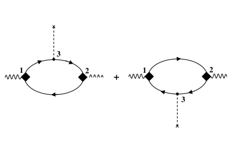
Figure 1: Three-point Green’s function describing the amplitude of the transition between the RPA states 1 and 2. The solid line presents the nucleon, the dashed one the single-particle external field $Q_{k}(x)$, and the wavy lines the transition densities.

The p-h structure of the state 1 (2) enters these graphs by means of the transition fields $v_{1(2)}(x)=\int F(xx^{\prime})\rho_{1(2)}(x^{\prime})\,dx^{\prime}$ with $\rho_{1(2)}(x)$ and $F(xx^{\prime})$ being the transition densities and the particle-hole interaction (depicted by the full diamonds), respectively. The transition fields are proportional to the residues in the poles of the effective operator : $\tilde{V}_{1(2)}(\omega)\simeq\displaystyle\frac{M_{1(2)}v_{1(2)}}{\omega-E_{1(2)}}$, with $\tilde{V}$ satisfying the equation [7]:

$$\tilde{V}(x,\omega)=V(x)+\int F(xx^{\prime})A(x^{\prime}x^{\prime\prime},\omega)\tilde{V}(x^{\prime\prime},\omega)\,dx^{\prime}dx^{\prime\prime},$$ (2)

Here, $A(xx^{\prime},\omega)$ is the free particle-hole propagator, carrying the quantum numbers of the appropriate p-h state, the probing single-particle operator $V_{1(2)}(x)$ has the matrix element $M_{1(2)}=\langle 1(2)|\hat{\cal V}_{1(2)}|0\rangle$ ($\hat{\cal V}=\sum_{a}V(x_{a})$).

The matrix element corresponding to the graphs is:

$$\hskip-28.45274pt\langle 2\|\hat{\cal Q}_{k}\|1\rangle=(-)^{J_{1}-k}\sum\limits_{345}\left\{\!\begin{array}[]{lll}J_{2}&k&J_{1}\\ j_{3}&j_{4}&j_{5}\end{array}\!\!\right\}\left[(-)^{J_{1}+J_{2}+k}\langle 4\|v_{2}^{+}\|5\rangle\langle 5\|Q_{k}\|3\rangle\langle 3\|v_{1}\|4\rangle\phantom{J^{J}}\right.$$ (5)

$$\hskip-28.45274pt\times\left(\frac{n_{4}(1-n_{5})(1-n_{3})}{(\varepsilon_{4}+E_{2}-\varepsilon_{5})(\varepsilon_{4}+E_{1}-\varepsilon_{3})}-\frac{(1-n_{4})n_{5}n_{3}}{(\varepsilon_{4}+E_{2}-\varepsilon_{5})(\varepsilon_{4}+E_{1}-\varepsilon_{3})}\right)$$

$$\hskip-28.45274pt-\langle 4\|v_{1}\|3\rangle\langle 3\|Q_{k}\|5\rangle\langle 5\|v_{2}^{+}\|4\rangle\left.\left(\frac{(1-n_{4})n_{5}n_{3}}{(\varepsilon_{4}-E_{2}-\varepsilon_{5})(\varepsilon_{4}-E_{1}-\varepsilon_{3})}-\frac{n_{4}(1-n_{5})(1-n_{3})}{(\varepsilon_{4}-E_{2}-\varepsilon_{5})(\varepsilon_{4}-E_{1}-\varepsilon_{3})}\right)\right],$$

with $n_{\lambda}$ and $\varepsilon_{\lambda}$ being occupation numbers and energies of the single-particle states, respectively ($\lambda$ is the set of the single-particle quantum numbers, $(\lambda)=\{lj\}$). The definition of the reduced single-particle matrix elements $\langle\lambda\|Q_{k}\|\mu\rangle$ by the Wigner-Eckart theorem is taken in accordance with Ref. [8].

The Eq. (5) can be transformed to express the transition amplitude in terms of the RPA $X$ and $Y$ amplitudes (see, e.g., Refs. [5, 9]):

$$\langle 2\|\hat{\cal Q}_{k}\|1\rangle=\sqrt{(2J_{1}+1)(2J_{2}+1)}\sum\limits_{345}(-)^{J_{1}+1+j_{4}+j_{3}}\left\{\!\begin{array}[]{lll}J_{2}&k&J_{1}\\ j_{3}&j_{4}&j_{5}\end{array}\!\!\right\}$$ (8)

$$\times\left[(-)^{J_{1}+J_{2}+k}\langle 5\|Q_{k}\|3\rangle\left(X^{(1)}_{34}X^{(2)}_{54}+(-)^{J_{1}+J_{2}+j_{3}+j_{5}}Y^{(1)}_{43}Y^{(2)}_{45}\right)\right.$$

$$\left.-\langle 3\|Q_{k}\|5\rangle\left(X^{(1)}_{43}X^{(2)}_{45}+(-)^{J_{1}+J_{2}+j_{3}+j_{5}}Y^{(1)}_{34}Y^{(2)}_{54}\right)\right]$$ (9)

with the use of the following representations for the $X$ and $Y$:

$$X^{(1)}_{21}=(-)^{j_{2}-j_{1}+J_{1}+1}\frac{\langle 2\|v_{1}\|1\rangle}{\sqrt{2J_{1}+1}}\frac{n_{1}(1-n_{2})}{(\varepsilon_{1}+E_{1}-\varepsilon_{2})}$$ (10)

$$Y^{(1)}_{21}=(-)^{j_{2}-j_{1}+1}\frac{\langle 1\|v_{1}\|2\rangle}{\sqrt{2J_{1}+1}}\frac{n_{1}(1-n_{2})}{(\varepsilon_{1}-E_{1}-\varepsilon_{2})}$$ (11)

One sees in Fig. 1 that there is an asymmetry between the vertex 1,2 (”dressed”) on the one hand and vertex 3 (”undressed”) on the other. This is because we have not incorporated effects of particle-hole interaction in channel 3, or, in other words, we neglected the effect of the virtual excitation of the corresponding giant multipole resonance. This effect has been well-known to play a crucial role in describing the neutron radiative capture since the model of direct-semidirect capture was suggested [10] (see also Ref. [11] for more recent developments). This additional contribution which takes into account virtual excitation of the giant resonance is shown in Fig. 2.

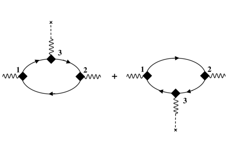
Figure 2: The generalized three-point Green’s function which takes into account the virtual excitation of multipole giant resonance in the channel 3.

The wavy line in the channel 3 depictures the total p-h propagator $\tilde{A}$ describing off-shell excitation of all p-h states (including the corresponding GR) with appropriate spin and parity. Using the fact that $\tilde{A}Q=A\tilde{Q}$, one can see that the sum of the graphs of Figs.1-2 is equivalent to the graphs of Fig.1 only if one replaces the external field $Q_{k}(x)$ by the corresponding effective field $\tilde{Q}_{k}(x,\omega)$ satisfying Eq.(2).

The Eq.(5) with the substitution $Q_{k}(x)\to\tilde{Q}_{k}(x,\omega)$ can be transformed further with the use of the spectral decomposition for the Green’s function of the single-particle radial Schrödinger equation $g_{(\lambda)}(rr^{\prime},\varepsilon)=\displaystyle\mathop{{\sum}^{\prime}}\limits_{\lambda}\frac{\chi_{\lambda}(r)\chi_{\lambda}(r^{\prime})}{\varepsilon-\varepsilon_{\lambda}}$ to include explicitly the single-particle continuum:

$$\langle 2\|\hat{\cal Q}_{k}\|1\rangle=(-)^{J_{1}-k}\left[\sum\limits_{4}n_{4}\left((-)^{J_{1}+J_{2}+k}G_{4}(E_{1},E_{2})+G_{4}^{T}(-E_{1},-E_{2})\right)\right.$$

$$\left.-\sum\limits_{3,5}n_{3}n_{5}\left((-)^{J_{1}+J_{2}+k}G_{3,5}(E_{1},E_{2})+G_{3,5}^{T}(-E_{1},-E_{2})\right)\right],$$ (12)

$$G_{4}(E_{1},E_{2})=\displaystyle\sum\limits_{(3)(5)}t_{(3)(4)(5)}(4|v_{2}^{+}\left(g_{(5)}(\varepsilon_{4}+E_{2})-\mathop{{\sum}^{\prime}}\limits_{5}n_{5}\frac{|5)(5|}{\varepsilon_{4}+E_{2}-\varepsilon_{5}}\right)$$

$$\times\tilde{Q}_{k}\displaystyle\left(g_{(3)}(\varepsilon_{4}+E_{1})-\mathop{{\sum}^{\prime}}\limits_{3}n_{3}\frac{|3)(3|}{\varepsilon_{4}+E_{1}-\varepsilon_{3}}\right)v_{1}|4),$$

$$G_{3,5}(E_{1},E_{2})=\sum\limits_{(4)}t_{(3)(4)(5)}\displaystyle\frac{(5|\tilde{Q}_{k}|3)}{\varepsilon_{5}-\varepsilon_{3}+E_{1}-E_{2}}(3|v_{1}(g_{(4)}(\varepsilon_{3}-E_{1})-g_{(4)}(\varepsilon_{5}-E_{2}))v_{2}^{+}|5),$$

$$t_{(3)(4)(5)}=\left\{\!\begin{array}[]{lll}J_{2}&k&J_{1}\\ j_{3}&j_{4}&j_{5}\end{array}\!\!\right\}\langle(4)\|v_{2}^{+}\|(5)\rangle\langle(5)\|Q_{k}\|(3)\rangle\langle(3)\|v_{1}\|(4)\rangle,$$ (15)

where we have decomposed the reduced matrix elements $\langle\lambda\|v\|\mu\rangle\equiv\langle(\lambda)\|v\|(\mu)\rangle(\lambda|v|\mu)$ into its spin-angular $\langle(\lambda)\|v\|(\mu)\rangle$ and radial $(\lambda|v|\mu)=\int\chi_{\lambda}(r)v(r)\chi_{\mu}(r)\,dr$ parts. The radial integrals (for brevity omitted) can be easily recovered, for instance,

$$(4|v_{2}^{+}g_{(5)}(\varepsilon_{4}+E_{2})\tilde{Q}_{k}g_{(3)}(\varepsilon_{4}+E_{1})v_{1}|4)=$$

$$\int\chi_{4}(r)v_{2}^{+}(r)g_{(5)}(rr^{\prime},\varepsilon_{4}+E_{2})\tilde{Q}_{k}(r^{\prime})g_{(3)}(r^{\prime}r^{\prime\prime},\varepsilon_{4}+E_{1})v_{1}(r^{\prime\prime})\chi_{4}(r^{\prime\prime})\,drdr^{\prime}dr^{\prime\prime}.$$

The superscript $T$ means transposition and $\mathop{{\sum}^{\prime}}$ runs over single-particle states with the same $l$ and $j$.

The Eq. (2) gives the general expression for the amplitude of the electromagnetic transitions within the CRPA. Apart from the single-particle continuum, it contains also contribution from the double phonon configurations. To see this, let us decompose the amplitude into ”direct” and ”semi-direct” parts according to the partition $\tilde{Q}_{k}=Q_{k}+(\tilde{Q}_{k}-Q_{k})$. The first, direct, part describes the amplitude in the single-phonon space and it has been only taken into account in all previous theoretical considerations [1]-[4]. As for the semi-direct part, the following approximate representation holds:

$$\tilde{Q}_{k}(x,\omega)-Q_{k}(x)\simeq\sum_{i}\frac{M_{i}q_{i}(x)}{\omega-\omega_{i}}.$$ (16)

with $q_{i}(x)$ being the transition fields for the doorway states forming the GDR. Thus, one can see, that the semi-direct part originates from admixtures of double-phonon configurations, like $|2\rangle+\sum_{i}\alpha_{i}|1\rangle\otimes|i\rangle$. The contribution to the transition amplitude is determined by both the matrix elements $M_{i}=\langle i|\hat{\cal Q}_{k}|0\rangle$ (states $|1\rangle$ or $|2\rangle$ serve as spectators in these electromagnetic transitions) and the admixture amplitudes $\alpha_{i}$.

It can be seen from Eqs. (2,16) that the mixing is described within first order perturbation theory with respect to the particle-hole interaction. Nevertheless, the approximation is satisfied in most cases due to the small values of the mixing amplitudes, that can be also seen from the calculated transition amplitudes being much less than the amplitude between the GDR and the ground state.

3 E1 transitions between the spin-dipole and Gamow-Teller resonances.

As an application of the approach described in the previous section, we calculate intensities and branching ratios for E1 decay of the charge-exchange spin-dipole resonance to some Gamow-Teller states (GTR and low-lying satellites) identified in Ref. [12]. To calculate the GT and SD strength distribution, we use the CRPA approach of Refs. [4, 13, 14]. The phenomenological isoscalar part of the nuclear mean field and the zero-range Landau-Migdal particle-hole interaction are the ingredients of the approach along with some selfconsistency conditions. The approach has allowed one to reproduce very well the experimental GTR energies in ⁹⁰Nb and ²⁰⁸Bi nuclei [14]. For each spin $J^{\pi}_{SDR}=(0^{-},1^{-})$ of the SD components we choose just one state with the maximal strength to be the SDR, lying at (26.6, 24.1) MeV in ²⁰⁸Bi and at (22.4, 20.1) MeV in ⁹⁰Nb, and for $J^{\pi}_{SDR}=2^{-}$ we choose three states with the maximal excitation energies, lying at (20.0, 21.3, 23.1) MeV in ²⁰⁸Bi and at (13.5, 14.4, 17.4) MeV in ⁹⁰Nb.

The details of the calculation of the effective fields for the SD and GT cases can be found in Refs. [4, 13, 14], and for the isovector dipole one - in Ref. [11]. In the latter case we take the velocity dependent particle-hole forces along with the isovector Landau-Migdal interaction that allows us to reproduce in the calculations both the experimental GDR energy and the observed excess of the energy-weighted sum rule over the TRK one. Because some transition energies are rather close to the GDR energy, the influence of the GDR spreading becomes important. We use the substitution $\omega\to\omega+{\rm i}\Gamma(\omega)/2$ in Eq. (2) to simulate the effect of GDR spreading (the mean energy-dependent doorway spreading width $\Gamma(\omega)$ has been chosen as in Ref. [11]).

We calculate the reduced matrix elements $\langle GTR\|\hat{\cal D}_{k}\|SDR,J\rangle$ according to Eq. (2) and Eq. (5) (with and without taking into account the virtual GDR excitation, respectively), and then the corresponding radiative widths $\Gamma_{\gamma}$ and $\Gamma_{\gamma}^{0}$ according to Eq. (1). The calculated widths for the E1 decay of the above-mentioned SD states to the GT states at the excitation energy $E_{GT}$ are listed in Table 1. The corresponding branching ratios are calculated as the ratio $\Gamma_{\gamma}/\Gamma^{\downarrow}$ with $\Gamma^{\downarrow}$ being the mean doorway-state spreading width chosen to reproduce the experimental total SDR width in the strength-function calculations ($\Gamma^{\downarrow}=4.7$ MeV for ²⁰⁸Bi [13], $\Gamma^{\downarrow}=4.$ MeV for ⁹⁰Nb).

Table 1: Calculated radiative widths and branching ratios for the E1 transitions between SDR and GT states in ⁹⁰Nb and ²⁰⁸Bi nuclei without ($\Gamma_{\gamma}^{0},b_{\gamma}^{0}$) and with ($\Gamma_{\gamma},b_{\gamma}$) taking into account the virtual GDR excitation, respectively.

	$E_{GT}$, MeV	$\Gamma_{\gamma}^{0}$, keV			$\Gamma_{\gamma}$, keV
Nucleus		($b_{\gamma}^{0}$, $\times 10^{-4}$)			($b_{\gamma}$, $\times 10^{-4}$)
	$\left/J^{\pi}_{SDR}\right.$	0-	1-	2-	0-	1-	2-
	8.9	3.40	1.03	0.10	3.68	0.02	0.008
90Nb		(8.5)	(2.6)	(0.3)	(9.2)	(0.05)	(0.02)
	0.0	0.21	0.10	0.08	1.62	0.13	0.37
		(0.5)	(0.2)	(0.2)	(4.0)	(0.3)	(0.9)
	15.5	2.28	0.70	0.09	6.49	0.03	0.008
		(4.9)	(1.5)	(0.2)	(13.8)	(0.05)	(0.02)
	9.3	0.15	0.03	0.14	0.80	0.43	0.22
		(0.3)	(0.05)	(0.3)	(1.7)	(0.9)	(0.5)
	8.1	0.24	0.02	0.04	1.05	0.26	0.16
		(0.5)	(0.03)	(0.08)	(2.3)	(0.5)	(0.3)
208Bi	6.4	0.23	0.007	0.001	0.58	0.04	0.03
		(0.5)	(0.01)	(0.002)	(1.2)	(0.1)	(0.06)
	4.9	1.05	0.0002	0.002	2.36	0.003	0.01
		(2.2)	(0.0005)	(0.003)	(5.0)	(0.007)	(0.03)
	4.5	0.50	0.0003	0.001	1.24	0.004	0.005
		(1.0)	(0.001)	(0.003)	(2.6)	(0.01)	(0.01)
	3.8	0.58	0.004	0.006	1.19	0.02	0.02
		(1.2)	(0.01)	(0.01)	(2.5)	(0.03)	(0.04)
	1.2	0.1	0.19	0.02	0.21	0.42	0.04
		(0.2)	(0.4)	(0.04)	(0.4)	(0.9)	(0.1)

As can be seen from the calculation results listed in the Table 1, taking into account of the virtual GDR excitation affects the results drastically. In the cases where the transition energy is well below the GDR energy, a destructive interference between the direct and semidirect parts of the amplitude always occurs, in agreement with both the qualitative description in terms of the effective charge [8] and previous quantitative consideration of Ref. [5]. In the cases when the transition energy is close to the GDR energy or exceeds it, the opposite situation takes place and one can see a significant enhancement of the corresponding amplitudes. This circumstance along with the steep $E_{\gamma}^{3}$ dependence of the E1 radiative width leads to the fact that the widths for SDR decay to some low-lying GT states can be comparable to those for SDR $\to$ GTR E1 transitions. Some of the calculated branching ratios are of order of $10^{-3}$, that seem to be accessible in experiments. In fact, the statistical background hinders detection of SDR $\to$ GTR decay, whereas it is small enough to allow detection of SDR decay to low-energy GT states which has been already observed in (³He,$t\gamma$) experiments on ²⁰⁸Pb [6]. For instance, strong gamma transitions have been observed to the unresolved GT states with E=3.8, 4.5, 4.9 MeV [6]. The energy of these gamma transitions (about 14 MeV) is very close to the energy of the GDR, and the predicted branching ratio ($\sim 10^{-3}$) can explain the observed transitions. However, we have to mention that the present calculations overestimate the mean energy of the SDR by about 2 MeV [13]. Bearing in mind strong energy-dependent renormalization of the transition amplitude found in this paper, this can lead to a noticeable difference between the calculated and observed branching ratios. We have not also taken the finite widths of the GTR and the SDR into consideration.

Special interest for testing the model lies in the E1 transition from the GTR to a 2.9 MeV 2^- SD state in ²⁰⁸Bi, which was observed recently at KVI [6]. The latter state has presumably a ($\pi 1h_{9/2})(\nu 1i_{13/2})^{-1}$ particle-hole structure and has a predicted excitation energy of 2.4 MeV. For this E1 transition we have found a large branching ratio $b_{\gamma}=4.3\cdot 10^{-3}$ due to the fact that the transition energy almost exactly coincides with the GDR energy, therefore we obtain maximal enhancement.

Finally, it is also worth to mention the sensitivity of the radiative widths to the spin of the SDR components due to their different energy position that could be in principle used to get experimentally information on their energy splitting.

4 Conclusion

A general continuum-RPA approach has been developed in the present paper to describe the intensities of electromagnetic transitions between different giant resonances. We have used a diagrammatic representation for the three-point Green’s function to derive the expression for the transition amplitude. The expression has allowed us to take the entire basis of particle-hole states into consideration as well as to incorporate important effects of mixing of single and double giant resonances. The radiative widths for E1 transition between the SDR and GT states (including GTR) have been calculated for ⁹⁰Nb and ²⁰⁸Bi nuclei. Some of the widths seem to be large enough to be accessible in experiments.

References

- [1] H. Sagawa, T. Suzuki, and N. van Giai, Phys. Rev. Lett. 75, 3629 (1995).
- [2] H. Sagawa, T. Suzuki, and N. van Giai, Phys. Rev. C 57, 139 (1998).
- [3] T. Suzuki and H. Sagawa, Eur. Phys. J. A9, 49 (2000).
- [4] V.A. Rodin, M.H. Urin, Phys. Rev. C 62, 067601 (2000).
- [5] V.Yu. Ponomarev, Ch. Stoyanov, N. Tsoneva, M. Grinberg, Nucl. Phys. A635, 470 (1998); Ch. Stoyanov, V.Yu. Ponomarev, N. Tsoneva, M. Grinberg, Nucl. Phys. A649, 93c (1999).
- [6] A. Krasznahorkay et al., KVI Annual Report (2002).
- [7] A.B. Migdal, Theory of finite Fermi-systems and properties of atomic nuclei, Moscow: Nauka, 1983 (in Russian).
- [8] A. Bohr, and B.R. Mottelson, Nuclear structure, Vol.1, New-York: Benjamin, 1969; Vol.2, New-York: Benjamin, 1975.
-
[9]
V.G. Soloviev, Theory of Complex Nuclei (Pergamon, Oxford, 1976);
Theory of Atomic Nuclei: Quasiparticles and Phonons (Inst. of Phys. Publ., Bristol, 1992). - [10] G.E. Brown, Nucl. Phys. 57, 339 (1964).
- [11] V.A. Rodin and M.H. Urin, Phys. Lett. B480 45 (2000).
- [12] A. Krasznahorkay et al., Phys. Rev. C 64, 067302 (2001).
- [13] E.A. Moukhai, V.A. Rodin, and M.H. Urin, Phys. Lett. B447, 8 (1999).
- [14] V.A. Rodin and M.H. Urin, Nucl. Phys. A687, 276c (2001).