The role of interaction vertices in bound state calculations

Abstract

In recent studies of the one and two-body Greens’ function for scalar interactions it was shown that crossed ladder and “crossed rainbow” (for the one-body case) exchanges play a crucial role in nonperturbative dynamics. In this letter we use exact analytical and numerical results to show that the contribution of vertex dressings to the two-body bound state mass for scalar QED are cancelled by the self-energy and wavefunction normalization. This proves, for the first time, that the mass of a two-body bound state given by the full theory can in a very good approximation be obtained by summing only ladder and crossed ladder diagrams using a bare vertex and a constant dressed mass. We also discuss the implications of the remarkable cancellation between rainbow and crossed rainbow diagrams that is a feature of one-body calculations.

1 Introduction

In general, a proper description of bound states requires an infinite summation of all possible interactions. Since this is usually not an easy task various approximation methods are used. Perhaps the best known approximations for the one-body and two-body systems are, respectively, the rainbow and the ladder approximations. The Dyson-Schwinger equation is usually used to sum the rainbow diagrams for the one-body propagator, and the Bethe-Salpeter equation in ladder approximation sums the two-body ladders exactly. In both cases these kernels do not sum any crossed exchanges. We now know that, for scalar theories, crossed ladder exchanges make a very significant contribution to the binding energies of two-body systems [1, 2], and that “crossed rainbow” diagrams make equally significant contributions to the one-body dressed mass [3]. This means that equations that include crossed exchanges approximately do a better job of reproducing the exact result than does the Bethe-Salpeter equation (in ladder approximation) or the Dyson-Schwinger equation (in rainbow approximation). In this letter our goals are (i) to study the role of vertex corrections in the two-body Greens’ function, and to (ii) to discuss the remarkable implication of the cancellation of rainbow and crossed rainbow diagrams in the one-body propagator. Here, and in the next section, we only discuss vertex corrections to the two-body Greens’ function, and return to the one-body propagator in Sec. III below.

In general a consistent treatment of any nonperturbative calculation must involve summation of all possible vertex corrections. Vertex corrections are those irreducible diagrams that surround an interaction vertex. Take $\phi^{3}$ theory as an example. The elementary vertex is the three-point vertex, $\Gamma_{3}$, but the particle interactions will lead to the appearance of $n$th order irreducable vertices, $\Gamma_{n}$, as illustrated in Fig. 1.

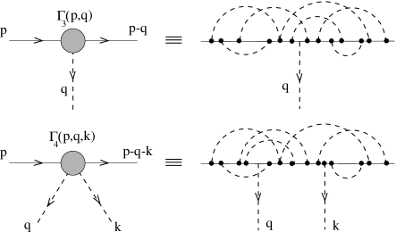
Figure 1: Because of the interactions, the one-particle irreducable vertex functions $\Gamma_{n}$ $(n=3,4,\cdots)$ depend on the external momenta.

The propagation of a bound state therefore involves a summation of all diagrams with the inclusion of higher order vertices (Fig. 2). A rigorous determination of all of these vertices is in general not feasible. In the literature on bound states $\Gamma_{n>3}$ interaction vertices are usually completely ignored. The 3-point vertex $\Gamma_{3}$ can be approximately calculated in the ladder approximation [4]. However a rigorous determination of the exact form of the 3-point vertex is difficult, for this requires the knowledge of even higher order vertices.

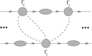
Figure 2: Exact computation of the two-body bound state propagator requires the summation of all particle self energies, vertex corrections, and ladder and crossed ladder exchanges.

In order to be able to make a connection between the exact theory and predictions based on approximate bound state equations it is essential that the role of interaction vertices be understood. The Feynman-Schwinger Representation (FSR) is a useful technique for this purpose. The FSR is an approach based on Euclidean path integrals similar to lattice gauge theory [1, 2, 3, 5, 6, 7, 8, 9, 10, 11, 12]. In this approach the path integrals over quantum fields are integrated out and replaced by path integrals over the trajectories of the particles.

In this paper we determine exactly the bound state mass for two scalar particles in scalar QED in the quenched approximation, i.e. neglecting only charge loop contributions, but including all self-energy, vertex and crossed ladder contributions. We in particular demonstrate, for the first time, that the full bound state result dictated by a Lagrangian can be well approximated by summing only generalized ladder diagrams (“generalized” ladders include crossed ladders and, in theories with an elementary four-point interaction, both overlapping and non-overlapping “triangle” and “bubble” diagrams). In the next section we investigate the interplay of vertex, self-energy and wave function normalizations within the context of massive scalar QED (SQED). First we look at the implications in 0+1 dimensions, where exact analytic results can be obtained using the FSR method. Next we extend the analysis to 3+1 dimensions using numerical methods, and show that in SQED₃₊₁ wave function normalization and vertex function normalization exactly cancel.

2 Determination of vertex contributions using the FSR approach

The Minkowski metric expression for the SQED Lagrangian in Feynman gauge is

$${\cal{L}}_{\rm SQED} = -m^{2}\chi^{2}-\frac{1}{4}F_{\mu\nu}^{2}+\frac{1}{2}\mu^{2}A_{\mu}^{2}-\frac{1}{2}(\partial^{\mu}A_{\mu})^{2}$$ (1)

$$+ (\partial_{\mu}-ieA_{\mu})\chi^{*}(\partial^{\mu}+ieA^{\mu})\chi\,,$$

where $A_{\mu}$ is the gauge field of mass $\mu$, $\chi$ is a charged field of mass $m$ and charge $e$, $F_{\mu\nu}=\partial_{\mu}A_{\nu}-\partial_{\nu}A_{\mu}$, and $A_{\mu}^{2}=A_{\mu}A^{\mu}$, $F_{\mu\nu}^{2}=F_{\mu\nu}F^{\mu\nu}$.

The final FSR result for the two-body propagator involves a quantum mechanical path integral that sums up contributions coming from all possible trajectories of the two charged particles $\chi$. This path integral is

$$G\simeq\bigg{\lmoustache}_{0}^{\infty}ds\,\,\bigg{\lmoustache}_{0}^{\infty}d\bar{s}\,\,\bigg{\lmoustache}\,({\cal D}z)_{xy}\,\bigg{\lmoustache}\,({\cal D}\bar{z})_{\bar{x}\bar{y}}e^{-K[z,s]-K[\bar{z},\bar{s}]}\langle W(C)\rangle\,,$$ (2)

where the particle trajectories $z_{i}(\tau)$ and $\bar{z}_{i}(\tau)$ are parametric functions of the parameter $\tau$, with endpoints $z_{i}(0)=x_{i}$, $\bar{z}_{i}(0)=\bar{x}_{i}$, $z_{i}(1)=y_{i}$, and $\bar{z}_{i}(1)=\bar{y}_{i}$, with $i=$1 to 4. The kinetic term is defined by

$$K[z,s] = m^{2}s+\frac{1}{4s}\int_{0}^{1}d\tau\,\dot{z}^{2}(\tau),$$ (3)

and the Wilson loop average $\langle W(C)\rangle$, obtained in this case by an analytic integration over the fields $A_{\mu}$, is

$$\langle W(C)\rangle = {\rm exp}\,\biggl{[}-\frac{e^{2}}{2}\int_{C}\,dz_{\mu}\,\int_{C}\,d\bar{z}_{\nu}\,\Delta_{\mu\nu}(z-\bar{z},\mu)\biggl{]},$$

$$\Delta_{\mu\nu}(x,\mu) = g_{\mu\nu}\bigg{\lmoustache}\frac{d^{4}p}{(2\pi)^{4}}\frac{e^{ipx}}{p^{2}+\mu^{2}}\,,$$

where the contour $C$ goes from $x\to y\to\bar{y}\to\bar{x}\to x$. In the numerical calculations the ultraviolet singularities are regulated by using a double Pauli-Villars subtraction

$$\Delta_{\mu\nu}(x,\mu) = g_{\mu\nu}\bigg{\lmoustache}\frac{d^{4}p}{(2\pi)^{4}}\frac{e^{ipx}(\Lambda_{1}^{2}-\mu^{2})(\Lambda_{2}^{2}-\mu^{2})}{(p^{2}+\mu^{2})(p^{2}+\Lambda_{1}^{2})(p^{2}+\Lambda_{2}^{2})}\,.$$

In the limit of large $z_{4}(1)=\bar{z}_{4}(1)=T$, the ground state mass is given by

$$M_{2}=\lim_{T\rightarrow\infty}-\frac{d}{dT}{\rm ln}[G(T)]=\frac{\int{\cal D}ZS^{\prime}[Z]e^{-S[Z]}}{\int{\cal D}Ze^{-S[Z]}}\,.$$ (4)

Equation (2) has a very nice physical interpretation. The term $\Delta_{\mu\nu}(z_{a}-z_{b},\mu)$ describes the propagation of gauge field interations between any two points on the particle trajectories, and the appearance of these interaction terms in the exponent means that the interactions are summed to all orders with arbitrary ordering of the points on the trajectories. Self-interactions come from terms with the two points $z_{a}$ and $z_{b}$ on the same trajectory, generalized ladder exchanges arise if the two points are on different trajectories, and vertex corrections arise from a combination of the two.

2.1 SQED₀₊₁

In order to understand the role of vertex corrections we first consider the simple case of SQED in 0+1 dimension. This interaction has been discussed in detail in Refs [2, 3, 9, 12].

In 0+1 dimension the FSR formulation yields the exact, analytic result for the $n$-body bound state interaction energy. It is

$$V_{\rm total} = V_{\rm self}+V_{\rm exchange}$$ (5)

$$= n\,\frac{e^{2}}{2\mu^{2}}-n\,(n-1)\,\frac{e^{2}}{2\mu^{2}}\,,$$

$$= -n\,(n-2)\,\frac{e^{2}}{2\mu^{2}}\,,$$ (6)

where the first term in (5) is from self-energy corrections, and the second from exchange contributions. The exact $n$-body dressed mass for SQED in 0+1 dimension is then [2, 3, 12]

$$M_{n} = n\,m+V_{\rm total}\,,$$ (7)

$$= n\,m-n\,(n-2)\,\frac{e^{2}}{2\mu^{2}}\,,$$

$$= n\,M_{1}+V_{\rm exchange}\,,$$ (8)

We emphasize that vertex corrections in the FSR approach are automatically taken into account by combinations of self energy and exchange interactions, and because these two interactions are additive in 0+1 dimension, the vertex corrections are identically zero! This fact is summarized in Eq. (8), which shows that the exact result for the $n$-body bound state can be written as the sum of $n$ dressed single particle masses plus energy arising from the generalized ladder exchanges (only).

In Fig. 3 we display the one-body and two-body bound state results. The figure shows the effects of higher order interaction vertices are included if one uses the dressed mass obtained from the original Lagrangian, the bare vertices with the original coupling strength $e$, and then sums all exchange interactions. This statement may be symbolically expressed by

$$L(e,\mu,m)\ +\ V_{\rm total} \longrightarrow L(e,\mu,M_{1})+V_{\rm exchange}$$ (9)

where $V_{\rm total}$ implies that all interactions are summed.

It might appear that these results are an oddity of 0+1 dimension. In the next section we will show that they also hold for 3+1 dimensions.

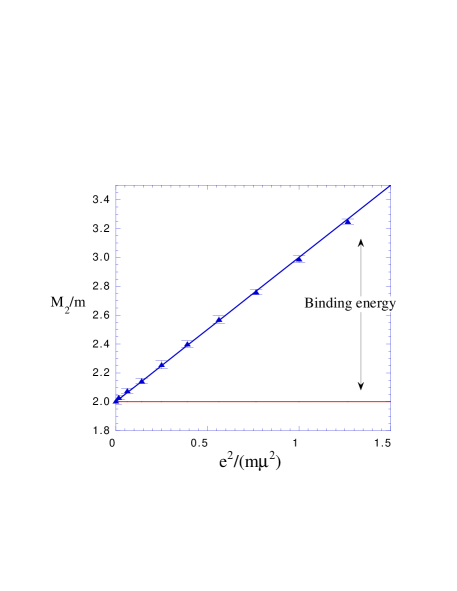
Figure 3: The two-body bound state mass for SQED in 0+1 dimension. The upper line is the theoretical result for 2$M_{1}$, with numerical results that agree with the analytic results, an important check. The lower line with $M_{2}/m$=2 is the analytical result for $M_{2}^{\rm exch}=M_{2}^{\rm tot}$. (Compare this with Fig. 4.)

2.2 SQED₃₊₁

We adopt the following procedure for determining the contribution of vertex corrections in 3+1 dimension. We start with an initial bare mass $m$ and calculate the full two-body bound state result with the inclusion of all interactions: generalized ladders, self energies and vertex corrections. Let us denote the result for the exact two-body bound state mass by $M_{2}^{\rm tot}(e^{2},m)$, since it will be a function of the coupling strength $e$ and the bare input mass $m$, and the superscript “tot” implies that all interactions are summed. Next we calculate the dressed one-body mass $M_{1}(e^{2},m)$. Then using the dressed mass value $M_{1}(e^{2},m)$ we calculate the bound state mass $M_{2}^{\rm exch}(e^{2},M_{1})$ by summing only the generalized exchange interaction contributions. In this last calculation we sum only exchange interactions (generalized ladders), but the self energy is approximately taken into account since we use the (constant) dressed one-body mass as input. However the vertex corrections and wavefunction renormalization are completely left out since we use the original vertex provided by the Lagrangian. In order to compare the full result where all interactions have been summed with the result obtained by two dressed particles interacting only by generalized ladder exchanges we plot the bound state masses obtained by these methods. Numerical results are presented in Fig. 4. This result is qualitatively similar to that obtained analytically for SQED in 0+1 dimension.

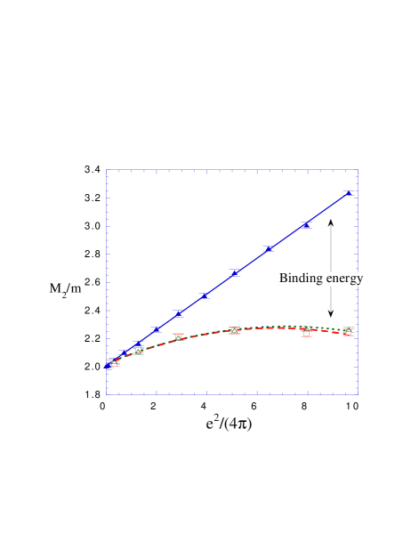
Figure 4: Two-body bound state mass for SQED in 3+1 dimensions. Solid triangles are 2$M_{1}$, open squares are $M_{2}^{\rm exch}$, and open triangles are $M_{2}^{\rm tot}$. Here $\mu/m=0.15$, $\Lambda_{1}/\mu=3$, and $\Lambda_{2}/\mu=5$. The smooth lines are fits to the “data”. Note that $M_{2}^{\rm exch}=M_{2}^{\rm tot}$ to within errors. (Compare this with Fig. 3.)

To summarize the analytical and numerical results we have presented here we give the following prescription for bound state calculations: In order to get the full result for bound states it is a good approximation to first solve for dressed one-body masses exactly (summing all generalized rainbow diagrams), and then use these dressed masses and the bare interaction vertex provided by the Lagrangian to calculate the bound state mass by summing only generalized ladder interactions (leaving out vertex corrections). In terms of Feynman graphs this prescription can be expressed as in Fig. 5

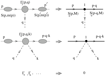
Figure 5: The correct two-body result can be obtained by simply using a dressed constituent mass and a bare vertex, and ignoring the contributions of higher order vertices.

3 Discussion

The significance of the results presented above rests in the fact that the problem of calculating exact results for bound state masses in SQED has been reduced to that of calculating only generalized ladders. Summation of generalized ladders can be addressed within the context of bound state equations [13, 14]. Here, for the first time, we have demonstrated the connection between the full prediction of a Lagrangian and the summation of generalized ladder diagrams. Our results are rigorous for SQED, but are only suggestive for more general theories with spin or internal symmetries. Since we have neglected charged particle loops (our results are in quenched approximation), and the current is conserved in SQED, it is perhaps not surprizing that the bare coupling is not renormalized, but the fact that the momentum dependence of the dressed mass and vertex corrections seem to cancel is surprizing and unexpected. If we were to unquench our calculation, or to use a theory without a conserved current, it is reasonable to expect that both the bare interaction and the mass would be renormalized.

Finally, we call attention to a remarkable cancellation that occurs in the one-body calculations. The exact self energies shown in Figs. 3 and 4 are nearly linear in $e^{2}$ [3]. This remarkable fact implies that the exact self energy is well approximated by the lowest order result from perturbation theory. It is instructive to see how this comes about. If we expand the self energy to fourth order, expanding each term about the bare mass $m$, we have

$$S^{-1}_{d}(p^{2}) = m^{2}-p^{2}+\Sigma(p^{2})$$ (10)

$$= m^{2}-p^{2}+\Sigma_{2}+(p^{2}-m^{2})\Sigma_{2}^{\prime}+\Sigma_{4}\,,\quad$$

where $\Sigma_{\ell}=\Sigma_{\ell}(m^{2})$ is the contribution of order $e^{\ell}$ evaluated at $p^{2}=m^{2}$, $\Sigma^{\prime}=d\Sigma(p^{2})/dp^{2}$ evaluated at $p^{2}=m^{2}$, and the formula is valid for $p^{2}-m^{2}\simeq e^{2}$. Expanding the dressed mass in a power series in $e^{2}$

$$M_{1}^{2} = m^{2}+m_{2}^{2}+m_{4}^{2}+\cdots\,,$$ (11)

where $m_{\ell}^{2}$ is the contribution of order $e^{\ell}$, and substituting into Eq. (10), give

$$M_{1}^{2} = m^{2}+\Sigma_{2}+\Sigma_{2}^{\prime}\Sigma_{2}+\Sigma_{4}+\cdots\,,$$ (12)

The mass is then

$$M_{1} = m+\frac{\Sigma_{2}}{2m}+\frac{4m^{2}\left[\Sigma_{2}^{\prime}\Sigma_{2}+\Sigma_{4}\right]-\Sigma_{2}^{2}}{8m^{3}}+\cdots\,,\qquad$$ (13)

The linearity of the exact result implies that the forth order term in Eq. (13) must be zero (or very small), and this can be easily confirmed by direct calculations!

The cancellation of the fourth order mass correction (and all higher orders) is reminisent of the cancellations between generalized ladders that explains why quasipotential equations are more effective that the ladder Bethe-Salpeter equation in explaining two-body binding energies. It shows that a simple evaluation of the second order self energy at the bare mass point is more accurate than solution of the Dyson Schwinger equation in rainbow approximation.

The general lesson seems to be that attempts to sum a small subclass of diagrams exactly is often less accurate than the approximate summation of a larger class of diagrams.

4 Acknowledgement

This work was supported in part by the US Department of Energy under grant No. DE-FG02-97ER41032. The Southeastern Universities Research Association (SURA) operates the Thomas Jefferson National Accelerator Facility under DOE contract DE-AC05-84ER40150.

References

- [1] T. Nieuwenhuis and J. A. Tjon, Phys. Rev. Lett. 77 (1996) 814.
- [2] T. Nieuwenhuis, PhD-thesis, University of Utrecht (1995), unpublished.
- [3] Ç Şavklı, F. Gross, and J. A. Tjon, Phys. Rev. D 62 (2000) 116006.
- [4] P. Maris, Nucl. Phys. Proc. Suppl. 90 (2000) 127.
- [5] T. Nieuwenhuis and J. A. Tjon, Phys. Lett. B 355 (1995) 283.
- [6] R. P. Feynman, Phys. Rev 80 (1950) 440; J. Schwinger, Phys. Rev. 82 (1951) 664.
- [7] Yu. A. Simonov, Nucl. Phys. B 307 (1988) 512.
- [8] Yu. A. Simonov, Nucl. Phys. B 324 (1989) 67.
- [9] Yu. A. Simonov and J. A. Tjon, Ann. Phys. 228 (1993) 1.
- [10] N. Brambilla and A. Vairo, Phys. Rev D. 56 (1997) 1445.
- [11] Ç. Şavklı, J. A. Tjon, and F. Gross, Phys. Rev. C 60 (1999) 055210; Erratum-ibid. C 61 (2000) 069901.
- [12] Ç. Şavklı Feynman-Schwinger technique in field theories, Series of lectures at the 13th Indian-Summer School, ”Understanding the Structure of Hadrons”, Prague, Czech Republic, August 28 - September 1, 2000.
- [13] F. Gross, Phys. Rev. 186 (1969) 1448; Phys. Rev. C 26 (1982) 2203.
- [14] D. R. Phillips, S. J. Wallace, and N. K. Devine, Phys. Rev. C 58 (1998) 2261.