Return of the EMC effect: finite nuclei

Abstract

A light front formalism for deep inelastic lepton scattering from finite nuclei is developed. In particular, the nucleon plus momentum distribution and a finite system analog of the Hugenholtz-van Hove theorem are presented. Using a relativistic mean field model, numerical results for the plus momentum distribution and ratio of bound to free nucleon structure functions for Oxygen, Calcium and Lead are given. We show that we can incorporate light front physics with excellent accuracy while using easily computed equal time wavefunctions. Assuming nucleon structure is not modified in-medium we find that the calculations are not consistent with the binding effect apparent in the data not only in the magnitude of the effect, but in the dependence on the number of nucleons.

I Introduction

The nuclear structure function $F_{2A}(x)$ is smaller than $A$ times the free nucleon structure function $AF_{2N}(x)$ for values of $x$ in the regime where valence quarks are dominant. This phenomenon, known as the European Muon Collaboration (EMC) effect Aubert:1983xm , has been known for almost twenty years. Nevertheless, the significance of this observation remains unresolved even though there is a clear interpretation within the parton model: a valence quark in a bound nucleon carries less momentum than a valence quark in a free one. There are many possible explanations, but no universally accepted one. The underlying mechanism responsible for the transfer of momentum within the constituents of the nucleus has not yet been specified. One popular mechanism involves ordinary nuclear binding which, in its simplest inculcation, is represented by evaluating the free nucleon structure function at a value of $x$ increased by a factor of the average separation energy divided by the nucleon mass $\bar{\epsilon}/M\simeq 0.04$. The validity of this binding effect has been questioned; see the reviews Arneodo:1992wf ; Geesaman:1995yd ; Piller:1999wx ; Frankfurt:nt .

The Bjorken variable $x$ is a fraction of the plus component of momentum, and the desire to obtain a more precise evaluation and understanding of the binding effect lead us to attempt to obtain a nuclear wave function in which the momentum of the nucleons is expressed in terms of this same plus component. Therefore we applied light front dynamics to determining nuclear wave functions previous . In this formalism one defines $x^{\pm}=x^{0}\pm x^{3}$ and quantizes on equal $x^{+}$ surfaces which have a constant light front time, $\tau$. The conjugate operator $P^{-}$ acts as an evolution operator for $\tau$. The plus momentum is canonically conjugate to the spatial $x^{-}$ variable. This light front formalism has a variety of advantages lcrev1 ; lcrev2 ; lcrev3 ; lcrev4 ; lcrev5 ; lcrev6 ; lcrev7 ; lcrev8 ; lcrev9 and also entails complications complications .

Our most recent result Miller:2001tg is that the use of the relativistic mean field approximation, and the assumption that the structure of the nucleon is not modified by effects of the medium, to describe infinite nuclear matter leads to no appreciable binding effect. The failure was encapsulated in terms of the Hugenholtz-van Hove theorem HvH which states that the average nuclear binding energy per nucleon is equal to the binding energy of a nucleon at the top of the Fermi sea. The light front version of this theorem is obtained from the requirement that, in the nuclear rest frame, the expectation values of the total plus and minus momentum are equal. The original version of the theorem was obtained in a non-relativistic theory in which nucleons are the only degrees of freedom. Here, the mesons are important and the theory is relativistic, but the theorem still holds. This theorem can be shown to restrict Miller:2001tg the plus momentum carried by nucleons to be the mass of the nucleus, which in turn implies that the probability for a nucleon to have a plus momentum $k^{+}$ is narrowly peaked about $k^{+}=M_{A}/A=\overline{M}$. Thus the only binding effect arises from the average binding energy, which is much smaller than the average separation energy. Therefore dynamics beyond the relativistic mean field approximation must be invoked to explain the EMC effect. This conclusion was limited to the case of infinite nuclear matter, and the computed nuclear structure function could only be compared with data on finite nuclear targets extrapolated to the limit $A\to\infty$. The goal of the present work is to extend the results to finite nuclei; the main complication arises from the spatial dependence of the nucleon and meson fields.

We briefly outline our procedure. In Sections II and III we present the covariant deep inelastic scattering formalism of Ref. Jung:1988jw and derive its representation in terms of nucleon single particle wave functions. The plus momentum distribution follows from this representation in Section IV where we also derive new version of the Hugenholtz-van Hove theorem. Then we present the results of analytic and numerical calculations in Section V, the latter giving an $A$ dependence of the ratio function contrary to experimental results. This again gives the result that the use of the relativistic mean field approximation, combined with the assumption that the nuclear medium does not modify the structure of the nucleon, cannot describe the EMC effect. The reasons for the subtle differences between the results for finite nuclei and nuclear matter are detailed in Section VI. Finally, we summarize and discuss possible implications.

II Nucleon Green’s Function for Finite Nuclei

We begin with the covariant plus momentum distribution function

$$f_{N}(y)=\int{d^{4}k\over(2\pi)^{4}}\delta\left(y-\frac{k^{0}+k^{3}}{\overline{M}}\right)\text{Tr}\left[\frac{\gamma^{+}}{2P^{+}A}\chi^{A}(k,P)\right]$$ (1)

where we identify

$$\chi^{A}(k,P) \equiv -i\int d^{4}x\int d^{4}ye^{-ik\cdot(x-y)}G^{C}(x,y),$$ (2)

where $G^{C}(x,y)$ is the connected part of the nucleon Green’s function:

$$iG(x,y) \equiv \langle P|T^{+}\{\psi^{\prime}(x)\overline{\psi}^{\prime}(y)\}|P\rangle.$$ (3)

This result is directly determined from the Feynman diagram in Fig. 1

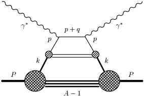
Figure 1: Feynman diagram for deep inelastic scattering. A nucleus of momentum $P$ is struck by a virtual photon of momentum $q$. We label nucleon momentum $k$, and quark momentum $p$.

following Ref. Jung:1988jw . So far this is independent of the particular relativistic mean field model, but for concreteness we use a Quantum Hadrodynamics (QHD) Lagrangian Serot:1997xg ; Serot:1986ey , specifically QHD-I as in Ref. Blunden:1999gq , where the nucleon fields, $\psi^{\prime}$, that appear in Eq. (3) are those appearing in the Lagrangian. Light front quantization requires that the plus component of all vector potential fields vanishes, and this is obtained by using the Soper-Yan transformation Soper:1971wn ; Yan:1973qf

$$\psi^{\prime}(x)\equiv e^{-ig_{v}\Lambda(x)}\psi(x),\qquad\partial^{+}\Lambda(x)=V^{+}(x).$$ (4)

to define the nucleon field operator $\psi$ for various models Miller:2001tg . This transformation allows the use of the eigenmode expansion for the $\psi$ fields which have been obtained previously in Ref. Blunden:1999gq

$$\psi(x) = \sum_{\alpha}\left[a_{\alpha}u_{\alpha}(x)+b_{\alpha}^{{\dagger}}v_{\alpha}(x)\right]$$ (5)

$$= \sum_{\alpha}\left[a_{\alpha}u_{\alpha}(\bm{x})e^{-ip^{-}_{\alpha}x^{+}/2}+b_{\alpha}^{{\dagger}}v_{\alpha}(\bm{x})e^{ip^{-}_{\alpha}x^{+}/2}\right],$$

where $a_{\alpha}$ and $b^{{\dagger}}_{\alpha}$ are (anti-)nucleon annihilation operators and we define $z\equiv-x^{-}/2$ with $\partial^{+}=2\partial_{-}=-\partial_{z}$ and $(\bm{x}_{\bot},z)\equiv\bm{x}$ which allows us to treat the minus and perpendicular coördinates on equal footing. The $u_{\alpha}$ and $v_{\alpha}$ are coördinate space 4-component spinor solutions to the light front Dirac equation with eigenvalues $p^{-}_{\alpha}/2=M-\varepsilon_{\alpha}$. To simplify the analysis we will temporarily ignore electromagnetic effects, but we will include them in the final numerical results. The light front mode equations in QHD-I are obtained by minimizing the $P^{-}$ operator (light front Hamiltonian) with the constraint Blunden:1999gq that $P^{+}=P^{-}$. The result is

$$-i\partial_{z}|\psi_{\alpha}^{-}\rangle = \left[\bm{\alpha}_{\bot}\cdot(\bm{p}_{\bot}-g_{v}\bar{\bm{V}}_{\bot})+\beta(M+g_{s}\phi)\right]|\psi_{\alpha}^{+}\rangle$$ (6)

$$p^{-}_{\alpha}|\psi_{\alpha}^{+}\rangle = \left[-i\partial_{z}+2g_{v}\bar{V}^{-}\right]|\psi_{\alpha}^{+}\rangle$$ (7)

$$+\left[\bm{\alpha}_{\bot}\cdot(\bm{p}_{\bot}-g_{v}\bar{\bm{V}}_{\bot})+\beta(M+g_{s}\phi)\right]|\psi_{\alpha}^{-}\rangle,$$

with

$$\quad u_{\alpha}(\bm{x}) = \sqrt{2P^{+}A}\;\langle\bm{x}|\psi_{\alpha}\rangle$$ (8)

$$\Lambda_{\pm}|\psi_{\alpha}\rangle = \frac{1}{2}\gamma^{0}\gamma^{\pm}|\psi_{\alpha}\rangle=|\psi_{\alpha}^{\pm}\rangle$$ (9)

$$\partial^{+}\bar{V}^{\mu} = \partial^{+}V^{\mu}-\partial^{\mu}V^{+}.$$ (10)

Using standard manipulations Serot:1986ey and defining $\varepsilon_{F}$ as the energy of the highest occupied state, we find the Green’s function to be

$$G(x,y) = \sum_{\alpha}u_{\alpha}(\bm{x})\overline{u}_{\alpha}(\bm{y})e^{-ig_{v}[\Lambda(\bm{x})-\Lambda(\bm{y})]}\int\frac{dk^{-}}{2\pi}e^{-ik^{-}(x^{+}-y^{+})/2}\left[\frac{1}{k^{-}-p^{-}_{\alpha}+i\varepsilon}+2\pi i\delta(k^{-}-p^{-}_{\alpha})\theta(\varepsilon_{F}-\varepsilon_{\alpha})\right]$$ (11)

$$\equiv G^{D}(x,y)+G^{C}(x,y),$$

where the superscripts $D$ and $C$ represent the disconnected and connected parts of the nucleon Green’s function, respectively. The connected part is relevant to deep inelastic scattering and is given by

$$G^{C}(x,y)=i\sum_{\alpha\in F}u_{\alpha}(\bm{x})\overline{u}_{\alpha}(\bm{y})e^{-ig_{v}[\Lambda(\bm{x})-\Lambda(\bm{y})]}e^{-ip^{-}_{\alpha}(x^{+}-y^{+})/2},$$ (12)

where the sum is over occupied levels $\alpha$ in the Fermi sea $F$. We now substitute Eq. (12) into Eq. (2), first defining $(\bm{k}_{\bot},k^{+})\equiv\bm{k}$ where $\bm{k}\cdot\bm{x}=\bm{k}_{\bot}\cdot\bm{x}_{\bot}+k^{+}z=\bm{k}_{\bot}\cdot\bm{x}_{\bot}-k^{+}x^{-}/2$, $d\bm{x}=d^{2}\bm{x}_{\bot}dz$, $d\bm{k}=d^{2}\bm{k}_{\bot}dk^{+}$ and

$$u^{\prime\prime}_{\alpha}(\bm{k})\equiv\int d\bm{x}e^{-i\bm{k}\cdot\bm{x}}e^{-ig_{v}\Lambda(\bm{x})}u_{\alpha}(\bm{x}).$$ (13)

We find

$$\chi^{A}(k,P)=(2\pi)^{2}\sum_{\alpha\in F}u^{\prime\prime}_{\alpha}(\bm{k})\overline{u}^{\prime\prime}_{\alpha}(\bm{k})\delta(k^{-}-p^{-}_{\alpha}).$$ (14)

The motivation for the ‘double-prime’ notation is the subject of the next section.

III Wave function Subtleties

It would be useful to express $\chi^{A}(k,P)$ in terms of solutions of the ordinary Dirac equation, because one may use a standard computer program cjht . To this end it is convenient rewrite Eq. (13)

$$\langle\bm{k}|\psi^{\prime\prime+}_{\alpha}\rangle=\int d\bm{x}e^{-i\bm{k}\cdot\bm{x}}e^{-ig_{v}\Lambda(\bm{x})}\langle\bm{x}|\psi^{+}_{\alpha}\rangle.$$ (15)

Note that the difference between $|\psi^{\prime\prime+}_{\alpha}\rangle$ of Eq. (15) and $u^{\prime\prime}_{\alpha}$ of Eq. (13) is simply the normalization factor $\sqrt{2P^{+}A}$. These ‘double-primed’ fields satisfy another version of the mode equations Eq. (6) and Eq. (7) following from an application of the Soper-Yan transformation Eq. (4), and are given by

$$\left[-i\partial_{z}-g_{v}V^{+}\right]|\psi_{\alpha}^{\prime\prime-}\rangle = \left[\bm{\alpha}_{\bot}\cdot(\bm{p}_{\bot}-g_{v}\bm{V}_{\bot})+\beta(M+g_{s}\phi)\right]|\psi_{\alpha}^{\prime\prime+}\rangle$$ (16)

$$\left[i\partial_{z}+g_{v}V^{+}-2g_{v}\bar{V}^{-}+p^{-}_{\alpha}\right]|\psi_{\alpha}^{\prime\prime+}\rangle = \left[\bm{\alpha}_{\bot}\cdot(\bm{p}_{\bot}-g_{v}\bm{V}_{\bot})+\beta(M+g_{s}\phi)\right]|\psi_{\alpha}^{\prime\prime-}\rangle.$$ (17)

If one multiplies Eq. (16) by $\gamma^{+}$ and Eq. (17) by $\gamma^{-}$ and adds the two equations, using $V^{+}=V^{-}=\bar{V}^{-}=V^{0}$, one obtains

$$\left[-\gamma^{3}(i\partial_{z}+p^{-}_{\alpha}/2)+\gamma^{0}(p^{-}_{\alpha}/2-g_{v}V^{0})\right]\psi_{\alpha}^{\prime\prime}(\bm{x})=\left[\bm{\gamma}_{\bot}\cdot\bm{p}_{\bot}+M+g_{s}\phi\right]\psi_{\alpha}^{\prime\prime}(\bm{x})$$ (18)

Eq. (18) is almost the same as the Dirac equation of the equal time formulation (for the $\psi^{\prime}$ fields), with the exception of the $p^{-}_{\alpha}$ term multiplying $\gamma^{3}$. Removing the offending term gives the relationship between the $\psi^{\prime}$ and $\psi^{\prime\prime}$ fields

$$\langle\bm{x}|\psi^{\prime}_{\alpha}\rangle \simeq e^{-ip^{-}_{\alpha}z/2}\langle\bm{x}|\psi^{\prime\prime}_{\alpha}\rangle$$ (19)

$$= e^{-ip^{-}_{\alpha}z/2}e^{-ig_{v}\Lambda(\bm{x})}\langle\bm{x}|\psi_{\alpha}\rangle$$ (20)

Eq. (20) is the approximate relationship between the $\psi$ and $\psi^{\prime}$ fields determined in Ref. Blunden:1999gq . The approximation lies in the fact that the spectrum condition is not maintained exactly, and the resulting Fourier transform of the wavefunction will have unphysical support for $k^{+}<0$. This support is largely irrelevant as it manifests far out on an exponential tail since $p^{-}_{\alpha}$ contains the nucleon mass. The relationship between the $\psi$ and $\psi^{\prime\prime}$ is exactly our definition Eq. (15). The use of Eq. (19) in Eq. (18) leads immediately to the result that the fields $\psi^{\prime}_{\alpha}$ satisfy the ordinary Dirac equation

$$\gamma^{0}(p^{-}_{\alpha}/2-g_{v}V^{0})\psi_{\alpha}^{\prime}(\bm{x})=\left[\bm{\gamma}\cdot\bm{p}+M+g_{s}\phi\right]\psi_{\alpha}^{\prime}(\bm{x})$$ (21)

We now are ready to derive a representation of Eq. (1) in terms of these nucleon wave functions.

IV Derivation of the Plus Momentum Distribution

In Ref. Blunden:1999gq , it was determined that a plus momentum distribution in QHD-I is given by

$$f(k^{+})=2\sum_{\alpha\in F}\int d^{2}\bm{x}_{\bot}\left|\langle\bm{x}_{\bot},k^{+}|\psi^{+}_{\alpha}\rangle\right|^{2}.$$ (22)

This distribution peaks at $k^{+}/\overline{M}\equiv y\simeq 0.8$ for ¹⁶O, (with smaller values for heavier nuclei) but is not the distribution obtained from the covariant formalism of Section II. The connection between this $f(y)$ and the covariant $f_{N}(y)$ was made in Ref. Miller:2001tg ; it was determined that, in the limit of infinite nuclear matter, the relationship between $f(y)$ and $f_{N}(y)$ is simply a shift in the argument by the vector meson potential:

$$f(y)=f_{N}(y+g_{v}V^{+}/\overline{M}).$$ (23)

This shift arises from the use of the Soper-Yan transformation Eq. (4) where the $\psi^{\prime}$ fields are those appearing in the Lagrangian and are used to determine $f_{N}(y)$, whereas the $\psi$ fields are used to determine $f(y)$. In finite nuclei, this relationship is somewhat more complicated since the vector meson potential is no longer a constant over all space. We start with Eq. (14), and see that

$$\text{Tr}\gamma^{+}\chi^{A}(k,P) = (2\pi)^{2}\sum_{\alpha\in F}\text{Tr}\left[\gamma^{+}u^{\prime\prime}_{\alpha}(\bm{k})\overline{u}^{\prime\prime}_{\alpha}(\bm{k})\right]\delta(k^{-}-p^{-}_{\alpha})$$

$$= 16\pi^{2}P^{+}A\sum_{\alpha\in F}\left|\langle\bm{k}|\psi^{\prime\prime+}_{\alpha}\rangle\right|^{2}\delta(k^{-}-p^{-}_{\alpha}).$$

Substituting into Eq. (1) we obtain

$$f_{N}(y) = \frac{2}{(2\pi)^{2}}\sum_{\alpha\in F}\int d\bm{k}\delta(y-k^{+}/\overline{M})\left|\langle\bm{k}|\psi^{\prime\prime+}_{\alpha}\rangle\right|^{2}.$$ (24)

Use of Parseval’s identity and integrating over $k^{+}$ gives us our main result:

$$f_{N}(y) = 2\overline{M}\sum_{\alpha\in F}\int d^{2}\bm{x}_{\bot}\left|\langle\bm{x}_{\bot},\overline{M}y|\psi^{\prime\prime+}_{\alpha}\rangle\right|^{2},$$ (25)

so the plus momentum distribution is related to Fourier transform of the $\psi^{\prime\prime}$ wave functions. One can see the similarity to Eq. (22); the difference lies entirely in Eq. (15). It should be emphasized that this result does not depend on the approximation in Section III.

We shall use $f_{N}(y)$ to compute the nuclear structure function $F_{2A}(x)$ in Section V, but first we derive a version of the Hugenholtz-van Hove theorem valid for finite nuclei. To do that, multiply Eq. (24) by $y$ and integrate

$$\langle y\rangle \equiv \int dyyf_{N}(y)$$ (26)

$$= \frac{2}{(2\pi)^{2}}\sum_{\alpha\in F}\int d\bm{k}\frac{k^{+}}{\overline{M}}\left|\langle\bm{k}|\psi^{\prime\prime+}_{\alpha}\rangle\right|^{2},$$

Now remove the plus projections and re-express $\psi^{\prime\prime}$ and its complex conjugate in coördinate spaces $\bm{x}$ and $\bm{x^{\prime}}$. One can then integrate over $\bm{k}$ yielding a delta function $\delta(\bm{x}-\bm{x^{\prime}})$ which allows integration over $\bm{x^{\prime}}$

$$\langle y\rangle = \frac{1}{\overline{M}}\sum_{\alpha\in F}\int d\bm{x}\psi^{\prime\prime{\dagger}}_{\alpha}(\bm{x})\gamma^{0}\gamma^{+}i\partial^{+}\psi_{\alpha}^{\prime\prime}(\bm{x})$$

We wish to look at the $\psi$ fields in order to understand our result in the context of Ref. Blunden:1999gq , so we need to perform the Soper-Yan transformation Eq. (4) and use $X^{{\dagger}}\gamma^{0}\equiv\overline{X}$

$$\langle y\rangle = \frac{1}{\overline{M}}\sum_{\alpha\in F}\int d\bm{x}\overline{\psi}_{\alpha}(\bm{x})\gamma^{+}[i\partial^{+}+g_{v}V^{+}(\bm{x})]\psi_{\alpha}(\bm{x})$$

If we explicitly put in the the nuclear state vectors, we can perform the sum on $\alpha$ by inserting creation and annihilation operators; we can add the time dependence for free since it is unaffected by $\partial^{+}$ and cancels with both fermion fields, and the vector potential is static. We have effectively undone the substitution Eq. (5) and now have an expectation value of an operator

$$\langle y\rangle = \frac{1}{M_{A}}\int d\bm{x}\langle\overline{\psi}\gamma^{+}[i\partial^{+}+g_{v}V^{+}]\psi\rangle$$ (27)

Using the vector meson field equation in QHD-I

$$\partial_{\mu}V^{\mu+}+m_{v}^{2}V^{+}=g_{v}\overline{\psi}\gamma^{+}\psi,$$

integrating by parts, and anti-symmetrizing one can re-express the second term of Eq. (27)

$$\langle y\rangle = \frac{1}{M_{A}}\int d\bm{x}\langle\overline{\psi}\gamma^{+}i\partial^{+}\psi+m_{v}^{2}V^{+}V^{+}+V^{+\mu}V_{\mu}^{\>\>+}\rangle$$ (28)

$$= \frac{1}{M_{A}}\int d\bm{x}\langle T^{++}-\partial^{+}\phi\partial^{+}\phi\rangle$$

$$= \frac{1}{M_{A}}\left(P^{+}-P^{+}_{s}\right)$$

$$= 1-\frac{P^{+}_{s}}{M_{A}}\simeq 1$$

where $T^{++}$ is the canonical energy momentum tensor, $P^{+}_{s}$ is the plus momentum of the scalar meson fields, and $P^{+}$ is the total nuclear plus momentum. The result Eq. (28) constitutes an analog of the Hugenholtz-van Hove theorem HvH for finite systems; the equality becomes exact in the nuclear matter limit, where the scalar meson contribution vanishes, as shown in our previous work Miller:2001tg . This means that we may anticipate that the binding effect will again be small. The ‘mixing’ of the vector operators and the scalar meson contribution will be elaborated on in a more general context in Section VI.

It is also worthwhile to explicitly evaluate the expression Eq. (25) for $f_{N}(y)$ in the limit of infinite nuclear matter. In this case, $V^{0}=V^{+}=V^{-}$ are constant and $\bm{V}_{\bot}=0$, so we find

$$\Lambda(z,\bm{x}_{\bot}) = \int_{z}^{\infty}dz^{\prime}V^{0}(z^{\prime},\bm{x}_{\bot})$$ (29)

$$= -V^{0}z$$

$$= -V^{+}z,$$

so that Eq. (15) becomes

$$\langle\bm{k}|\psi^{\prime\prime+}_{\alpha}\rangle = \int d\bm{x}e^{-i\bm{k}_{\bot}\cdot\bm{x}_{\bot}}e^{-i(k^{+}-g_{v}V^{+})z}\langle\bm{x}|\psi^{+}_{\alpha}\rangle$$ (30)

$$= \langle\bm{k}_{\bot},k^{+}-g_{v}V^{+}|\psi^{+}_{\alpha}\rangle.$$

Therefore Eq. (25) becomes

$$f_{N}(y) = 2\overline{M}\sum_{\alpha\in F}\int d^{2}\bm{x}_{\bot}\left|\langle\bm{x}_{\bot},\overline{M}y-g_{v}V^{+}|\psi^{+}_{\alpha}\rangle\right|^{2},$$ (31)

which is simply the expression (22) modified by a shift in the argument of $g_{v}V^{+}/\overline{M}$. Thus we find Eq. (23) is satisfied in the nuclear matter limit. It is important to stress that all that is recovered here is the shift in the argument and not any particular form of the plus momentum distribution which arises from the specific model used.

V Nuclear Structure Functions

We determine the wave functions appearing in Eq. (25) numerically from a relativistic self-consistent treatment following Horowitz and Serot Horowitz:1981xw using the same program cjht which includes electromagnetic effects. The plus momentum distribution follows and is given in Fig. 2 for ¹⁶O, ⁴⁰Ca, ²⁰⁸Pb and in the nuclear matter limit (the ¹⁶O calculation is also shown in Fig. 4). One can see that the peaks appear near $y=1$ as required by the Hugenholtz-van Hove theorem Eq. (28).

Figure 2: Plus momentum distributions, $f_{N}(y)$, for ⁴⁰Ca (solid), ¹⁶O (short dashes), ²⁰⁸Pb (dot-dashes) and nuclear matter (long dashes).

It is worth noting that application of the Soper-Yan transformation Eq. (4) to the $\psi^{\prime\prime}$ wavefunctions obtained from the equal time wavefunctions reproduces the plus momentum distributions, including the correct asymmetry, of the light front calculations in Ref. Blunden:1999gq , which did not use the approximation Eq. (19), as shown in Fig. 3 for Oxygen and nuclear matter.

Figure 3: $f(y)$ distributions for ¹⁶O and nuclear matter after application of the Soper-Yan transformation. Note that the peaks occur at $y<1$.

This demonstrates the excellence of the approximation relating light front and equal time wavefunctions. One can see that the effect in finite nuclei of the Soper-Yan transformation is to shift and broaden the plus momentum distribution, while in nuclear matter it is just a shift. If these distributions were to be used in the nuclear structure function Eq. (33) though, since $\langle y\rangle\simeq 0.8$ for Oxygen, the ratio function Eq. (35) would fall precipitously to nearly zero at $x\simeq 0.6$ in stark contradiction with experiment.

We also evaluated the plus momentum distribution Eq. (25) with the simple non-relativistic harmonic oscillator shell model as an additional check on our method. These (equal time) wavefunctions give us an explicit, although approximate in the sense of Section III, closed form of the plus momentum distribution for ¹⁶O:

$$f_{N}(y) \simeq \frac{\xi}{\sqrt{16\pi}}[e^{-\xi^{2}(\eta_{1s}-y)^{2}}$$ (32)

$$+2\left(1+\xi^{2}(\eta_{1p}-y)^{2}\right)e^{-\xi^{2}(\eta_{1p}-y)^{2}}],$$

with $\eta_{nl}=M+\omega(2(n-1)+l+3/2)-v_{0}$ where $v_{0}\simeq 50\text{ MeV}$, and $\xi\equiv\overline{M}b$ where $b=(m\omega)^{-1/2}\simeq 1.6\text{ fm}$ is the oscillator length which is fit to the root mean square radius of Oxygen $\langle R^{2}\rangle^{1/2}\simeq 2.7\text{ fm}$. The distribution Eq. (32) narrows for larger $\xi$ which corresponds to an increasing root mean square radius. This distribution is plotted in Fig. 4 where one can see that it peaks near $y=1$ like the relativistic Hartree calculation, but appears to have a smaller value of $\langle y\rangle$.

Figure 4: Plus momentum distribution for ¹⁶O calculated with harmonic oscillator (solid curve) and relativistic Hartree (dashed curve) wave functions.

It is worth noting that the Hartree calculations are in the relativistic equal time framework and put into our relativistic light front formalism, while the harmonic oscillator calculations are non-relativistic and put into our relativistic formalism.

The structure function is given by the convolution

$$\frac{F_{2A}(x_{A})}{A}=\int_{x_{A}}^{A}dyf_{N}(y)F_{2N}(x_{A}/y),$$ (33)

with $x_{A}\equiv Q^{2}A/2P\cdot q=xM/\overline{M}$. The assumption that nuclear effects do not modify the structure of the nucleon is embodied in Eq. (33) by the use of the structure function of a free nucleon; we use the parameterization deGroot:yb

$$F_{2N}(x)=0.58\sqrt{x}(1-x)^{2.8}+0.33\sqrt{x}(1-x)^{3.8}+0.49(1-x)^{8}.$$ (34)

The experiments measure the ratio function, defined as

$$R(x)=\frac{F_{2A}(x_{A})}{AF_{2N}(x)}.$$ (35)

The results of our calculations are plotted for ¹⁶O, ⁴⁰Ca, ²⁰⁸Pb and in the nuclear matter limit in Fig. 5 showing data for Carbon, Calcium and Gold from SLAC-E139 Gomez:1993ri and an extrapolation Sick:1992pw for the nuclear matter calculation.

Figure 5: Ratio functions for ¹⁶O, ⁴⁰Ca and ²⁰⁸Pb showing data for Carbon, Calcium and Gold, respectively, from SLAC-E139 Gomez:1993ri . The nuclear matter calculation shows extrapolated data Sick:1992pw .

The most striking result is that these calculations fail to reproduce the EMC effect; the curves consistently miss the minima in the data, and the agreement gets worse with increasing $A$. Another important result is that the ratio function does not fall to zero as would be the case if the small effective mass ($\sim 0.56M$ for nuclear matter in QHD-I) were the relevant parameter describing the binding effect which would follow from using Eq. (22) instead of Eq. (25). The results also show a minimum near $x\simeq 0.6$ for Oxygen and nuclear matter that is deeper than the Calcium and Lead calculations. This is a curious feature that contradicts the trend in experimental data, and is due to the effects of two parameters.

The first, and most important, is that of the location of the peak of the plus momentum distribution given by Eq. (28), which gradually approaches $y=1$ as the nuclear matter limit is reached. This is due to the fact that scalar mesons carry a small amount of plus momentum Blunden:1999gq that vanishes as $A\rightarrow\infty$. The closer to $y=1$ the peak is in Fig. 2, the less pronounced the minimum in Fig. 5, all else remaining constant. The second effect is due to $\overline{M}$, which reaches a minimum at ⁵⁶Fe corresponding to a more pronounced minimum of the ratio function than for $A<56$ or $A>56$, keeping the scalar meson contribution constant.

Using a Gaussian parameterization of the plus momentum distribution and the experimental binding energy per nucleon via the semi-empirical mass formula, we have modeled the dependence of the minimum of the ratio function, $R(x\simeq 0.72)$, on the number of nucleons in the nucleus in Fig. 6.

Figure 6: $R(x=0.72)$ as a function of $A$ including scalar meson and binding effects (solid line), and leaving binding energy per nucleon constant at $-8.5\text{ MeV}$ (dashed line). The data are from SLAC-E139 Gomez:1993ri .

The motivation for the use of Gaussian plus momentum distributions is based on the expansion Frankfurt:nt

$$F_{2A}(x_{A}) = F_{2N}(x_{A})+\epsilon x_{A}F_{2N}^{\prime}(x_{A})$$ (36)

$$+\gamma[2x_{A}F_{2N}^{\prime}(x_{A})+x_{A}^{2}F_{2N}^{\prime\prime}(x_{A})]$$

$$\text{where }\epsilon \equiv 1-\int dyyf_{N}(y)$$ (37)

$$\gamma \equiv \int dy(y-1)^{2}f_{N}(y)$$ (38)

The Gaussian parameterization uses the peak location and width, $\langle y\rangle$ and $(\langle y^{2}\rangle-\langle y\rangle^{2})^{1/2}$ respectively, from the relativistic Hartree calculations in Fig. 2, and is normalized to unity. This allows us to obtain a plus momentum distribution for any $A$ with minimal effort. We show the combined effect of scalar mesons and binding energy per nucleon on the ratio function along with the effect of scalar mesons alone using a constant binding energy per nucleon of $-8.5\text{ MeV}$ independent of $A$. It can be seen that a changing $\overline{M}$ with $A$ has the most effect for nuclei much larger than Iron, but does not change the general trend that the minimum of the ratio function becomes less pronounced as $A$ increases due to the vanishing scalar meson contribution and the peak of the plus momentum distribution approaching unity. This dependence of the binding effect on $A$ is quite different, both in magnitude and shape, than the trend in experimental data summarized in Ref. Sick:1992pw which satisfies $R(x\simeq 0.72)\sim A^{-1/3}$, so that the minimum becomes more pronounced as $A$ increases. This fully demonstrates the inadequacy of conventional nucleon-meson dynamics to explain the EMC effect.

VI Scalar Meson Contribution to Plus Momentum and More General Considerations

The average value of $y$, given by Eq. (28), yields the nucleon contribution to the plus momentum, and is less than one which can be seen in Fig. 2. We now address the remaining plus momentum in finite nuclei. Previous results Blunden:1999gq show that a small fraction ($\delta y\sim 0.005$) of the plus momentum is carried by the scalar mesons which vanishes as the nuclear matter limit is approached. This is due to the fact that scalar mesons couple to gradients in the scalar density (arising mainly from the surface of finite nuclei) which vanish as $A\rightarrow\infty$. The question is: why are scalar mesons allowed to carry plus momentum and not vector mesons?

The simplest answer lies in the Dirac structure of Eq. (1); the $\gamma^{+}$ in the trace picks out terms in the full interacting Green’s function with an odd number of gamma matrices which includes all Lorentz vector interactions and excludes Lorentz scalar interactions. The Dirac structure of $f_{N}(y)$ is directly related to the Dirac structure of the energy momentum tensor, so the answer also lies there and illuminates a problem with conventional nucleon-meson dynamics. The component of the energy momentum tensor relevant to the plus momentum, from a chiral Lagrangian containing isoscalar vector mesons, scalar mesons and pions, is given by Miller:1997cr ; Miller:1999ap

$$T^{++} = V^{+\mu}V_{\mu}^{\>\>+}+m_{v}^{2}V^{+}V^{+}+\overline{\psi}\gamma^{+}i\partial^{+}\psi+\partial^{+}\phi\partial^{+}\phi$$ (39)

$$+\partial^{+}\bm{\pi}\cdot\partial^{+}\bm{\pi}+\bm{\pi}\cdot\partial^{+}\bm{\pi}\frac{\bm{\pi}\cdot\partial^{+}\bm{\pi}}{\pi^{2}}(1-\frac{f^{2}}{\pi^{2}}\sin^{2}\frac{\pi}{f}).$$

Since each of the terms in Eq. (39) involves one of the fields, it is natural to associate each term with a particular contribution to the plus momentum. This decomposition, though, is not well defined; field equations relate various components. We see the first three terms of Eq. (39) appear in $\langle y\rangle$, which defines the nucleon contribution to the total nuclear plus momentum, in the derivation of the Hugenholtz-van Hove theorem Eq. (28); we are not allowed to have the vector mesons contribute a well defined fraction of plus momentum. This means that one could trade certain mesonic degrees of freedom for nucleons by replacing mesonic vertices with nucleon point couplings, for example, in line with the general concept of effective field theory. In our case the first three terms are related by the vector meson field equation, but the fourth is left out since the scalar mesons couple to the scalar density $\overline{\psi}\psi$ which is not present in Eq. (39). Therefore the scalar mesons (and pions) contribute a well defined fraction of plus momentum. These explicit meson contributions create an EMC binding effect, but the pionic contributions are also limited by nuclear Drell-Yan experiments Alde:1990im to carrying about 2% of the plus momentum which is insufficient to account for the entire EMC effect which corresponds to about 5% of the plus momentum for Iron.

VII Summary and Discussion

The minimum in the EMC effect is known to have a monotonically decreasing behavior with $A$, which has been studied in Refs. Gomez:1993ri ; Sick:1992pw among others. Our present theory is defined by the use of the mean-field approximation, along with the assumption that nuclear effects do not modify the structure of the nucleon. This theory leads to results in severe disagreement with experiment. Not only do we find that the depth of the minimum is monotonically decreasing with $A$, but it has a smaller magnitude than experiment. These results, which fail to capture any of the important features of the experiments, represent a failure of relativistic mean field theory. Furthermore, the plus momentum distributions we compute give $\langle y\rangle\simeq 1$ which indicates that nearly all of the plus momentum is carried by the nucleons. In order to reproduce the data, the nucleon plus momentum must be decreased by some mechanism that becomes more important at larger $A$. Nucleon-nucleon correlations cannot take plus momentum from nucleons, and explicit mesonic components in the nuclear Fock state wavefunction carrying plus momentum are limited Bickerstaff:1984ax ; Ericson:1984vt ; Berger:1986dr by Drell-Yan experiments Alde:1990im . Thus it appears that the EMC effect may be due to something outside of conventional nucleon-meson dynamics. For example, true modifications to nucleon structure caused by nuclear interactions could be important, in which case one would need to use models such as the mini-delocalization model Frankfurt:nt , quark-meson coupling (QMC) model Saito:1994ki ; Benhar:1999up ; Gross:1992pi or the chiral quark soliton model reviewed in Diakonov:2000pa to include those effects.