Effects of momentum conservation on the analysis of anisotropic flow

Abstract

We present a general method for taking into account correlations due to momentum conservation in the analysis of anisotropic flow, either by using the two-particle correlation method or the standard flow vector method. In the latter, the correlation between the particle and the flow vector is either corrected through a redefinition (shift) of the flow vector, or subtracted explicitly from the observed flow coefficient. In addition, momentum conservation contributes to the reaction plane resolution. Momentum conservation mostly affects the first harmonic in azimuthal distributions, i.e., directed flow. It also modifies higher harmonics, for instance elliptic flow, when they are measured with respect to a first harmonic event plane such as one determined with the standard transverse momentum method. Our method is illustrated by application to NA49 data on pion directed flow.

I Introduction

In heavy ion collisions, the transverse momenta of outgoing particles are correlated with the direction of the impact parameter (reaction plane) of the two incoming nuclei. For example, at energies above 100 MeV per nucleon, nucleons in the projectile rapidity region are deflected away from the target. This collective effect is usually referred to as directed (or sidewards) flow. It is characterized by the first Fourier coefficient of the particle azimuthal distribution, $v_{1}$ Voloshin:1996mz :

$$v_{1}\equiv\left\langle\cos(\phi-\Phi_{RP})\right\rangle,$$ (1)

where $\phi$ denotes the azimuthal angle of an outgoing particle, $\Phi_{RP}$ is the azimuth of the reaction plane, and angular brackets denote an average over events and over all particles in a given transverse momentum and rapidity window. Differential flow is characterized by $v_{1}(p_{T},y)$ that describes the directed flow in a narrow transverse momentum ($p_{T}$) and rapidity ($y$) interval.

The most common observable to quantify directed flow, introduced by Danielewicz and Odyniec in 1985 Danielewicz:1985hn , is the mean transverse momentum projected on the reaction plane, $\left\langle p_{x}\right\rangle$, as a function of rapidity. In terms of $v_{1}$, it can be written as $\left\langle p_{x}\right\rangle=\left\langle p_{T}\,v_{1}(p_{T},y)\right\rangle$, where the average in the right-hand side is taken over $p_{T}$. This observable is believed to be sensitive to the nuclear compressibility and to in-medium cross sections Magestro:ba . Experimentally, $\left\langle p_{x}\right\rangle$ is extracted from azimuthal correlations between the outgoing particles, under the assumption that these correlations are only due to flow. However, it was soon realized that global momentum conservation also induces azimuthal correlations. Different ways to correct for this effect were devised in Refs. Danielewicz:1988in ; ogilvie . These methods are still in use at intermediate Cussol:2001df ; Prendergast:2000fv as well as at relativistic energies Ahle:jv ; E895 ; Crochet:1997hz . Generally, corrections are important for weak flow and/or small systems, when there are physical or detector differences between the forward and backward hemispheres in a reaction.

More detailed information can be obtained on the physics involved in the collision by studying the transverse momentum dependence of directed flow Pan:1992ef , $v_{1}(p_{t})$ in a given rapidity window. Detailed theoretical studies have been presented for this differential directed flow Li:1996iz ; Li:1999bh ; Li:2000bj . This was accompanied by new analyses of experimental data, and a wealth of results are now available from FOPI at SIS FOPI , E877 at AGS E877 and NA49 at CERN NA49 . In these analyses, unfortunately, correlations arising from momentum conservation are not taken into account. Recently, it was shown Borghini:2000cm that they may in fact be of the same order of magnitude as correlations due to flow, leading to a reevaluation of the “standard” flow analysis results.

In this paper, we show how to modify standard flow analysis techniques in order to take into account momentum conservation. Two flow methods are used experimentally. The first one relies on a study of two-particle correlations Wang:1991qh . This simple case is discussed in Sec. II. The second method, which is by far the most common, involves the construction of a “flow vector” used as an estimate of the reaction plane Danielewicz:1985hn ; Poskanzer:1998yz . In order to measure the flow of a particle, one correlates it to the estimated event plane of the flow vector, and corrects this correlation by dividing by a “resolution” factor which takes into account the uncertainty of the reaction plane determination. This procedure is recalled in Sec. III. In Sec. IV, we show how this method can be modified to take into account momentum conservation.

The momentum conservation leads to two effects, whose magnitude is controlled by a parameter $f$ which is roughly the square root of the fraction of all particles used in the estimate of the event plane. First, momentum conservation contributes to the correlation between a particle and the flow vector, proportionally to the parameter $f$ (Sec. IV.2). This spurious correlation can be eliminated through a redefinition of the flow vector (Sec. IV.1). In addition, momentum conservation affects the resolution of the event plane, although the effect is smaller, as it is quadratic in $f$ (Sec. IV.3). This second effect may also bias higher harmonics measured with respect to the first harmonic event plane. (Note, however, that momentum conservation has no effect when elliptic flow is measured with respect to the second harmonic event plane.) Our results are discussed in Sec. V; in particular, we show that the correlation from momentum conservation vanishes if the detector acceptance is symmetric with respect to midrapidity, because particles belonging to the forward and backward hemispheres are given weights with opposite signs. In Sec. VI, the method is illustrated by NA49 data on pion directed flow. Finally, technical details are exposed in the Appendixes A and B.

II Two-particle correlation technique

Since the orientation of the reaction plane is not known, $v_{1}$ is extracted from azimuthal correlations between outgoing particles. The simplest way consists in using two-particle azimuthal correlations Wang:1991qh . These are related to $v_{1}$ by the identity:

$$\left\langle\cos(\phi_{1}-\phi_{2})\right\rangle = \left\langle\cos(\phi_{1}-\Phi_{RP})\cos(\phi_{2}-\Phi_{RP})\right\rangle$$ (2)

$$= \left\langle\cos(\phi_{1}-\Phi_{RP})\right\rangle\left\langle\cos(\phi_{2}-\Phi_{RP})\right\rangle$$ (3)

$$= v_{1}(1)\,v_{1}(2),$$ (4)

where $v_{1}(1)$ and $v_{1}(2)$ denote the flow coefficients associated with each particle. For spherical nuclei, symmetry with respect to the reaction plane ensures that the $\left\langle\sin(\phi-\Phi_{RP})\right\rangle$ terms are zero. In going from the first to the second line, we have assumed that all azimuthal correlations are due to flow or, equivalently, that azimuthal angles with respect to the reaction plane $\phi_{1}-\Phi_{RP}$ and $\phi_{2}-\Phi_{RP}$ are statistically independent. Recent implementations of the two-particle correlation method can be found in Refs. Prendergast:2000fv ; Lacey:2001 .

As recalled in the introduction, however, there are also azimuthal correlations induced by global momentum conservation, so that the measured correlation is in fact the sum of two terms(when both effects are small)

$$\left\langle\cos(\phi_{1}-\phi_{2})\right\rangle=v_{1}(1)v_{1}(2)+\left\langle\cos(\phi_{1}-\phi_{2})\right\rangle_{\rm mom.\ cons.},$$ (5)

where the last term, due to momentum conservation, is evaluated in Appendix A of Ref. Borghini:2000cm :

$$\left\langle\cos(\phi_{1}-\phi_{2})\right\rangle_{\rm mom.\ cons.}=-\frac{{p_{T}}_{1}{p_{T}}_{2}}{N\left\langle p_{T}^{2}\right\rangle},$$ (6)

where $N$ denotes the total number of particles produced in the collision, and the average value $\left\langle p_{T}^{2}\right\rangle$ is similarly taken over all produced particles. Since one usually detects only a fraction of the produced particles, the denominator of Eq. (6) should be estimated using a model, or by an extrapolation of available data to full phase space.

In order to take into account the correlations due to momentum conservation in the analysis of directed flow, one simply subtracts the contribution due to momentum conservation, Eq. (6), from the measured two-particle correlation Eq. (5), so as to isolate the correlation due to flow. This is the procedure followed in Ref. Borghini:2000cm to estimate the effects of momentum conservation on the analysis of directed flow at SPS.

III Flow-vector method

Most analyses of directed flow rely on the construction of the event flow-vector Danielewicz:1985hn ; Poskanzer:1998yz defined as:

$${\bf Q}=\sum_{j=1}^{N}w_{j}{\bf u}_{j},$$ (7)

where the sum runs over all produced particles, ${\bf u}_{j}$ denotes the unit vector of the particle transverse momentum, ${\bf u}_{j}={\bf e_{x}}\cos\phi_{j}+{\bf e_{y}}\sin\phi_{j}={\bf p_{T}}_{j}/{p_{T}}_{j}$, and $w_{j}$ is a weight depending on the particle type, its transverse momentum ${p_{T}}_{j}$ and rapidity $y_{j}$. The weights, $w_{j}$, are usually given non zero values only in regions of good detector acceptance.

The azimuthal angle of the flow vector, $\Phi$, is considered an estimate of the reaction plane azimuth, $\Phi_{RP}$. Therefore, the azimuthal angle of ${\bf Q}$ with respect to the reaction plane is usually referred to as the uncertainty in the reaction plane determination, and will be denoted by $\Delta\Phi\equiv\Phi-\Phi_{RP}$. One then writes an equation similar to Eq. (2) for the azimuthal correlation between a particle with azimuth $\phi$ and the flow vector:

$$\left\langle\cos(\phi-\Phi)\right\rangle = \left\langle\cos(\phi-\Phi_{RP}-\Phi+\Phi_{RP})\right\rangle$$ (8)

$$= \left\langle\cos(\phi-\Phi_{RP})\right\rangle\left\langle\cos\Delta\Phi\right\rangle$$ (9)

$$= v_{1}\left\langle\cos\Delta\Phi\right\rangle.$$ (10)

This equation once again relies on the assumption that azimuthal correlations are only due to flow. To avoid autocorrelation one should subtract the contribution of the particle under study from the flow vector. Since the flow vector, Eq. (7), involves a summation over many particles, the correlation between a particle and the flow vector, Eq. (8), is usually much stronger than the correlation between two particles, Eq. (2). This is one of the main reasons why the flow vector method is more commonly used. However, correlations due to momentum conservation are also stronger, so that corrections due to momentum conservation are of the same magnitude with both methods, as we shall see in Sec. V. In the rest of this paper $\Phi_{RP}$ will be taken as zero; that is, the reaction plane is along the $x$-axis.

The next step in the analysis is to evaluate the “resolution” $\left\langle\cos\Delta\Phi\right\rangle$. This factor results from a competition between flow, which tends to align ${\bf Q}$ in the direction of the reaction plane, and statistical fluctuations, whose relative magnitude decreases like $1/\sqrt{N}$. A quantitative estimate can be obtained with help of the central limit theorem. This theorem allows one to write the distribution of the flow vector as a Gaussian distribution in the coordinate system where the orientation of the reaction plane is fixed Voloshin:1996mz ; Ollitrault:1992bk :

$$\frac{dP}{d{\bf Q}}=\frac{1}{\pi\sigma^{2}}\exp\left(-\frac{({\bf Q}-\left\langle\bf Q\right\rangle)^{2}}{\sigma^{2}}\right).$$ (11)

The average value $\left\langle\bf Q\right\rangle$ is aligned with the reaction plane, i.e., with the $x$-axis, while the dispersion $\sigma$ is due to statistical fluctuations. Writing ${\bf Q}=Q({\bf e_{x}}\cos\Delta\Phi+{\bf e_{y}}\sin\Delta\Phi)$, and integrating over $Q$ and $\Delta\Phi$, one obtains Poskanzer:1998yz ; Ollitrault:1997di :

$$\left\langle\cos\Delta\Phi\right\rangle=\frac{\sqrt{\pi}}{2}\chi\,e^{-\chi^{2}/2}\left[I_{0}(\chi^{2}/2)+I_{1}(\chi^{2}/2)\right],$$ (12)

where $I_{0}$, $I_{1}$ are modified Bessel functions and $\chi$ is the dimensionless parameter $\chi\equiv\left\langle\bf Q\right\rangle\cdot{\bf e_{x}}/\sigma$, which characterizes the relative magnitude of flow and statistical fluctuations. In what follows, $\chi$ will be referred to as the “resolution parameter” .

This parameter $\chi$ is usually estimated from the correlation between two “subevents” Danielewicz:1985hn : the set of $N$ particles is divided randomly into two equivalent subsets of $N/2$ particles, labeled $a$ and $b$. One then constructs two flow vectors ${\bf Q_{a}}$ and ${\bf Q_{b}}$ defined as in Eq. (7), with the summation running over the corresponding subset. Flow induces an azimuthal correlation between ${\bf Q_{a}}$ and ${\bf Q_{b}}$, since both are correlated with the reaction plane. Then, when all azimuthal correlations are due to flow, the distribution of $\Phi_{a}-\Phi_{b}$ depends only on the resolution parameter $\chi$. To find the functional form of this relationship, one writes the probability distribution of ${\bf Q_{a}}$ in a form similar to Eq. (11):

$$\frac{dP}{d{\bf Q_{a}}}=\frac{1}{\pi\sigma_{a}^{2}}\exp\left(-\frac{({\bf Q_{a}}-\left\langle\bf Q_{a}\right\rangle)^{2}}{\sigma_{a}^{2}}\right),$$ (13)

and a similar formula for ${\bf Q_{b}}$ with $\left\langle\bf Q_{b}\right\rangle=\left\langle\bf Q_{a}\right\rangle\equiv\left\langle\bf Q_{\rm sub}\right\rangle$ and $\sigma_{b}=\sigma_{a}\equiv\sigma_{\rm sub}$ since the subevents are equivalent. The distribution of the relative angle $dP/d(\Phi_{a}-\Phi_{b})$ depends only on the resolution parameter associated with either subevent $\chi_{\rm sub}\equiv\left\langle\bf Q_{\rm sub}\right\rangle\cdot{\bf e_{x}}/\sigma_{\rm sub}$. Its analytic expression can be found in Refs. Ollitrault:1997di ; Ollitrault:ba , and provides a perfect fit to experimental data Taranenko:1999yh . The parameter $\chi_{\rm sub}$ is usually obtained from the square root of the average cosine of the relative angle, $\sqrt{\left\langle\cos(\Phi_{a}-\Phi_{b})\right\rangle}$, which is simply the resolution of a subevent plane, and is given by Eq. (12) with $\chi$ replaced by $\chi_{\rm sub}$. Equation (12) must then be inverted in order to obtain $\chi_{\rm sub}$ Poskanzer:1998yz . In a simpler way, $\chi_{\rm sub}$ can be obtained directly from the fraction of events with the relative angle between subevents $|\Phi_{a}-\Phi_{b}|$ larger than $\pi/2$ Ollitrault:1997di ; Ollitrault:ba :

$$P(|\Phi_{a}-\Phi_{b}|>\pi/2)=\frac{1}{2}e^{-\chi_{\rm sub}^{2}}.$$ (14)

This method is used for example in Ref. Taranenko:1999yh . If $\chi_{\rm sub}$ is significantly larger than unity, however, only a small fraction of events have $|\Phi_{a}-\Phi_{b}|$ larger than $\pi/2$, and the resulting statistical error on $\chi_{\rm sub}$ is larger than with the previous method. In the limiting case $\chi_{\rm sub}\gg 1$, the distribution of the relative angle $\Phi_{a}-\Phi_{b}$ is a Gaussian, and $\chi_{\rm sub}$ can be directly obtained from its width, $\left\langle(\Phi_{a}-\Phi_{b})^{2}\right\rangle=1/\chi_{\rm sub}^{2}$.

The last step is to relate the parameter $\chi_{\rm sub}$, corresponding to one subevent, to $\chi$, corresponding to the whole event. Since each subevent contains half of the particles, $\left\langle\bf Q_{\rm sub}\right\rangle=\left\langle\bf Q\right\rangle/2$. If correlations between particles are only due to flow, a similar scaling occurs in the statistical fluctuations: $\sigma_{\rm sub}^{2}=\sigma^{2}/2$, so that

$$\chi=\chi_{\rm sub}\sqrt{2}.$$ (15)

The flow-vector method is defined by Eqs. (8), (12), (15), and a technique for obtaining $\chi_{\rm sub}$. Equations (8), (14), and (15), must be modified when taking into account momentum conservation. This is studied in Sec. IV.

The first harmonic flow vector, Eq. (7), can also be used to measure higher harmonics of the azimuthal distribution $v_{n}=\left\langle\cos n\phi\right\rangle$ for $n>1$, with the help of an equation similar to Eq. (8):

$$\left\langle\cos n(\phi-\Phi)\right\rangle=v_{n}\left\langle\cos n\Delta\Phi\right\rangle.$$ (16)

The corresponding resolution $\left\langle\cos n\Delta\Phi\right\rangle$ depends on the same parameter $\chi$ Poskanzer:1998yz ; Ollitrault:1997di . This method has been used to analyze elliptic flow $v_{2}$ elliptic relative to a first harmonic event plane. Since, as we have mentioned above, momentum conservation modifies the value of $\chi$, it must also be taken into account in this case. We come back to this discussion in Sec. V.

IV Modifications due to momentum conservation

Global momentum conservation induces correlations between outgoing particles and the flow vector. In the same way as Eq. (2) is replaced by Eq. (5), Eq. (8) becomes

$$\left\langle\cos(\phi-\Phi)\right\rangle=v_{1}\left\langle\cos\Delta\Phi\right\rangle+\left\langle\cos(\phi-\Phi)\right\rangle_{\rm mom.\ cons.}.$$ (17)

There are two methods to take into account the additive term. The first one consists in redefining the ${\bf Q}$-vector [i.e., modify $\Phi$ in Eq. (17)] in each event, in such a way that the additional term no longer appears (Sec. IV.1). Alternatively, one can compute explicitly the additive term and subtract it in order to isolate the correlation due to flow (Sec. IV.2). Furthermore, momentum conservation affects the resolution $\left\langle\cos\Delta\Phi\right\rangle$, and the methods used to estimate the resolution must be modified accordingly (Sec. IV.3).

IV.1 Shifted flow-vector method

The correlation due to momentum conservation between the flow vector and a particle with momentum ${\bf p_{T}}$ can be characterized by the average value of ${\bf u}\cdot{\bf Q}$, where ${\bf u}\equiv{\bf p_{T}}/p_{T}$. Using the definition of the ${\bf Q}$-vector, Eq. (7), and the expression of the two-particle correlation due to momentum conservation, Eq. (6), one obtains:

$$\left\langle{\bf u}\cdot{\bf Q}\right\rangle_{\rm mom.cons.}=-p_{T}\,\frac{\left\langle wp_{T}\right\rangle}{\left\langle p_{T}^{2}\right\rangle},$$ (18)

where averages in the right-hand side run over all the produced particles. This suggests one could redefine the flow vector as

$${\bf Q^{\prime}}={\bf Q}+\frac{\left\langle wp_{T}\right\rangle}{\left\langle p_{T}^{2}\right\rangle}{\bf p_{T}},$$ (19)

so that momentum conservation does not contribute to the correlation between ${\bf Q^{\prime}}$ and the particle under study. As a matter of fact, when there is no flow the shifted flow vector ${\bf Q^{\prime}}$ and ${\bf p_{T}}$ are now uncorrelated by momentum conservation: any correlation between ${\bf Q^{\prime}}$ and ${\bf p_{T}}$ arises from flow, because here and throughout the paper, we neglect other sources of nonflow correlations.

A similar method was proposed in Ref. ogilvie , in the context of intermediate-energy collisions, where the shifted flow vector was defined as

$${\bf Q^{\prime}}={\bf Q}+\frac{\sum_{j}w_{j}m_{j}/{p_{T}}_{j}}{\sum_{j}m_{j}}{\bf p_{T}},$$ (20)

where $m_{j}$ is the mass of particle $j$. If $\left\langle p_{T}^{2}\right\rangle$ of different particles scales with their mass $m$, our definition Eq. (19) reduces approximately to Eq. (20). That is the case in particular for a thermalized nonrelativistic gas at rest with (almost) no flow, as in Ref. ogilvie . However, Eq. (20) is no longer valid when there is flow, and/or relativistic effects, whereas Eq. (19) still holds.

IV.2 Explicit subtraction

Instead of modifying the flow vector event-by-event, one can as well keep the original definition, Eq. (7), and subtract the contribution of momentum conservation to the measured correlations, Eq. (17), at the end of the analysis.

Let us first estimate the order of magnitude of the last term of Eq. (17). We assume for simplicity that the particle under study has no flow, $v_{1}=0$, so that only the correlation due to momentum conservation remains. We then make the following approximation:

$$\left\langle\cos(\phi-\Phi)\right\rangle_{\rm mom.\ cons.}=\left\langle\frac{{\bf u}\cdot{\bf Q}}{Q}\right\rangle\sim\frac{\left\langle{\bf u}\cdot{\bf Q}\right\rangle}{\left\langle Q\right\rangle},$$ (21)

with ${\bf u}\equiv{\bf p_{T}}/p_{T}$. The average dot product is given by Eq.(18). Furthermore, the average length of the flow vector $\left\langle Q\right\rangle$ is approximately equal to the r.m.s. length $\sqrt{\left\langle Q^{2}\right\rangle}$. Neglecting correlations between momenta, one obtains from the definition, Eq. (7), $\left\langle Q^{2}\right\rangle\sim N\left\langle w^{2}\right\rangle$. All in all, the order of magnitude of the correlation due to momentum conservation, Eq. (21), reads

$$\left\langle\cos(\phi-\Phi)\right\rangle_{\rm mom.\ cons.}\sim-\frac{p_{T}}{\sqrt{N\left\langle p_{T}^{2}\right\rangle}}\,f,$$ (22)

where $f$ is a dimensionless quantity given by

$$f \equiv \frac{\left\langle wp_{T}\right\rangle}{\sqrt{\left\langle w^{2}\right\rangle\left\langle p_{T}^{2}\right\rangle}}$$ (23)

$$= \left\langle wp_{T}\right\rangle_{Q}\sqrt{\frac{M}{\left\langle w^{2}\right\rangle_{Q}N\left\langle p_{T}^{2}\right\rangle}},$$ (24)

and the subscript $Q$ refers to those $M$ particles used for the ${\bf Q}$-vector (for which weight $w_{i}\neq 0$). The weight $w$ vanishes for particles not seen in the detector, so that $\left\langle w^{2}\right\rangle$ and $\left\langle wp_{T}\right\rangle$ scale like the fraction of detected particles. Hence, $f$ scales like the square root of the fraction of detected particles. This is seen more clearly in the second line of Eq. (23) where there is a factor $\sqrt{M/N}$. If $w$ is taken as $+1$ for particles detected in the forward hemisphere and $-1$ for the backward hemisphere, then $\left\langle wp_{T}\right\rangle_{Q}=(M_{F}\left\langle p_{T}\right\rangle_{F}-M_{B}\left\langle p_{T}\right\rangle_{B})/M$, where $F$ and $B$ refer to particles used for the $\bf{Q}$-vector from the forward and backward hemispheres, respectively, so that $M=M_{F}+M_{B}$. In this case the quantity $\left\langle w^{2}\right\rangle_{Q}=1$.

The estimate in Eq. (22) is only an order of magnitude. A more accurate expression can be obtained under very general assumptions. We show in Appendix A that the actual value of the correlation due to momentum conservation between a particle and the flow vector is

$$\left\langle\cos(\phi-\Phi)\right\rangle_{\rm mom.\ cons.}=$$ (25)

$$\displaystyle-\frac{p_{T}}{\sqrt{N\left\langle p_{T}^{2}\right\rangle}}\,\frac{f}{\sqrt{1-f^{2}}}\,\frac{\sqrt{\pi}}{2}e^{-\chi^{2}/2}I_{0}(\chi^{2}/2),$$ (26)

where $\chi\equiv\left\langle\bf Q\right\rangle\cdot{\bf e_{x}}/\sigma$ has been defined in Sec. III. It is worth noting that the Eq. (25) result now depends on $\chi$, expressing the effect of flow in reducing the correlation due to momentum conservation. However, the dependence is weak for small $\chi$ (i.e., in the case of poor resolution).

IV.3 Correction to the reaction plane resolution

We now discuss the influence of momentum conservation on the determination of the resolution parameter $\chi$. The corrections discussed below hold for the method of Sec. IV.1 as well as for the method of Sec. IV.2.

As recalled in Sec. III, the resolution is determined from the correlation between subevents, i.e., from the distribution of the relative angle $\Phi_{a}-\Phi_{b}$ between the subevents. We show in Appendix B that momentum conservation contributes to this correlation such that the distribution of $\Phi_{a}-\Phi_{b}$ now depends both on the resolution parameter of the subevent $\chi_{\rm sub}$, and on the parameter $f$ introduced in Eq. (23), in a non trivial way: taking into account momentum conservation does not only amount to changing the value of $\chi_{\rm sub}$. This is because the shape of the distribution of the relative angle $\Phi_{a}-\Phi_{b}$ depends on whether the correlation is due to flow or to other effects. This is illustrated in Ref. Ollitrault:dy , where the distribution of $\Phi_{a}-\Phi_{b}$ is plotted in the two limiting cases when the correlations are only due to flow ($f=0$), or only to other, nonflow effects ($\chi_{\rm sub}=0$).

As recalled in Sec. III, there are several methods of extracting $\chi_{\rm sub}$ from the distribution of $\Phi_{a}-\Phi_{b}$. The usual method relies on the calculation of $\langle\cos(\Phi_{a}-\Phi_{b})\rangle$. If $f$ is much smaller than unity, Eq. (12) becomes:

$$\left\langle\cos(\Phi_{a}-\Phi_{b})\right\rangle^{1/2}=$$ (27)

$$\displaystyle\frac{\sqrt{\pi}}{2}\,e^{-\chi_{\rm sub}^{2}/2}\left[\chi_{\rm sub}^{2}\left[I_{0}(\chi_{\rm sub}^{2}/2)+I_{1}(\chi_{\rm sub}^{2}/2)\right]^{2}\right.$$ (28)

$$\displaystyle-\left.\frac{f^{2}}{2}\left[I_{0}^{2}(\chi_{\rm sub}^{2}/2)+I_{1}^{2}(\chi_{\rm sub}^{2}/2)\right]\right]^{1/2},$$ (29)

Once the left-hand side and $f$ are known, $\chi_{\rm sub}$ can be obtained by solving this equation. This expression holds only to leading order in $f$. We were not able to obtain an analytic formula for arbitrary $f$.

It may be simpler to extract $\chi_{\rm sub}$ from the fraction of events for which $|\Phi_{a}-\Phi_{b}|>\pi/2$. Then, the correction for momentum conservation can be implemented using the following exact formula, derived in Appendix B:

$$P(|\Phi_{a}-\Phi_{b}|>\pi/2)=\frac{1}{2-f^{2}}e^{-\chi_{\rm sub}^{2}},$$ (30)

instead of Eq. (14). If the resolution parameter is large, $\chi_{\rm sub}>1$, this method leads to larger statistical errors as recalled in Sec. III. If $\chi_{\rm sub}\gg 1$, the distribution of $\Phi_{a}-\Phi_{b}$ is Gaussian and $\chi_{\rm sub}$ can be obtained from its width:

$$\left\langle(\Phi_{a}-\Phi_{b})^{2}\right\rangle=\frac{2}{\chi_{\rm sub}^{2}(2-f^{2})}.$$ (31)

Finally, the relation between the resolution parameter of the subevent, $\chi_{\rm sub}$, and that of the whole event, $\chi$, is easily obtained using Eqs. (43), (49), and the scaling relation $\left\langle\bf Q_{\rm sub}\right\rangle=\left\langle\bf Q\right\rangle/2$:

$$\chi=\chi_{\rm sub}\sqrt{\frac{2-f^{2}}{1-f^{2}}}.$$ (32)

When correlations are weak (i.e., when both $f$ and $\chi$ are small compared to unity), the event plane resolution can be corrected for momentum conservation through the following simple formula:

$$\chi^{2}({\rm corrected})=\chi^{2}({\rm uncorrected})+f^{2}.$$ (33)

This approximation can be used instead of Eqs. (27)/(30) and (32) on the $\chi$ of the full event plane as obtained in Sec. III.

Let us summarize the results obtained in this Section. The crucial parameter, which determines the magnitude of corrections due to momentum conservation, is the dimensionless parameter $f$, defined in Eq. (23). Once this quantity has been estimated, the subevent plane resolution parameter, $\chi_{\rm sub}$, can be obtained from either $\left\langle\cos(\Phi_{a}-\Phi_{b})\right\rangle$ using Eq. (27), if $f\ll 1$, or from the fraction of subevent angle differences greater than $\pi/2$ using Eq. (30). Or, if the resolution parameter is very large, from Eq. (31). The full event plane resolution parameter, $\chi$, is obtained from Eq. (32), and the full event plane resolution from Eq. (12). Finally, subtracting from the measured values of $\left\langle\cos(\phi-\Phi)\right\rangle$ the contribution due to momentum conservation, Eq. (25), and dividing the result by the event plane resolution, one obtains the final $v_{1}$ values. When $f$ vanishes, one recovers the formulas of the standard flow analysis, recalled in Sec. III.

V Discussion

Corrections arising from momentum conservation are twofold. First, they contribute to the correlation between a particle and the event plane. This contribution, which increases linearly with the particle transverse momentum Borghini:2000cm , must be subtracted from the measured correlation so as to isolate the correlation due to flow; see Eq. (17). Next, momentum conservation affects the resolution of the event plane, which results in a global multiplicative factor. Both effects must be taken into account in the analysis of directed flow, but only the second one in the case of higher harmonics relative to a first harmonic event plane.

All effects of momentum conservation disappear if the parameter $f$ defined in Eq. (23) vanishes, which occurs if $\left\langle wp_{T}\right\rangle=0$. Since $w$ is usually an odd function of the center-of-mass rapidity Danielewicz:1985hn , $\left\langle wp_{T}\right\rangle$ vanishes as soon as the detector acceptance is symmetric with respect to midrapidity, as was already mentioned in Refs. Danielewicz:1988in ; Poskanzer:1998yz . Another theoretically interesting limit is the case when all particles are detected and, in particular, when $w=p_{T}$, which implies $f=1$. In this case, the flow vector, Eq. (7), is the sum of all transverse momenta, which vanishes due to momentum conservation. This is why the corrections derived in the previous Section diverge when $f$ goes to unity.

When the weight keeps a constant sign, the correction due to momentum conservation is of the same relative magnitude within the flow vector method [Eq. (17)] as within the two-particle method [Eq. (5)]. In the latter method, the correlation due to flow is of order $v_{1}^{2}$ while the correlation due to momentum conservation is of order $1/N$. The flow vector method enhances both terms by a factor of order $\sqrt{M}$, where $M$ is the number of particles within the detector acceptance, which are used in constructing the flow vector ${\bf Q}$. Roughly speaking, this is because the flow vector is analogous to a random walk of $M$ steps: the length of the walk is approximately $\sqrt{M}$ times the size of a step, and similarly the correlation between ${\bf Q}$ and a given particle is $\sqrt{M}$ times the correlation between two particles. This can be seen more explicitly from the formulas derived above. We first estimate the correlation due to flow, i.e., the first term in the right-hand side of Eq. (17). Since $\left\langle\cos\Delta\Phi\right\rangle$ is proportional to $\chi$ for small $\chi$ (see Eq. (12) and the figures in Refs. Poskanzer:1998yz ; Ollitrault:1997di ), and $\chi\sim v_{1}\sqrt{M}$, this term is indeed of order $v_{1}^{2}\sqrt{M}$. Let us now estimate the second term, whose order of magnitude is given by Eq. (22). We choose for simplicity a weight $w=p_{T}$ within the detector acceptance, and zero outside. The parameter $f$ in Eq. (23) then reduces to $f\simeq\sqrt{M/N}$. Introducing this value in the estimate Eq. (22), we find a correlation of order $\sqrt{M}/N$, as expected.

The correction to the reaction plane resolution, on the other hand, is generally of order $f^{2}$, which is roughly the fraction of the total number of particles used in estimating the reaction plane. Note that the correction to the resolution is not the same for all harmonics of the azimuthal distribution. Indeed, the resolution $\left\langle\cos n\Delta\Phi\right\rangle$ is more sensitive to $\chi$ when $n>1$, so that effects are larger for higher harmonics relative to the first harmonic event plane.

Let us now discuss how the corrections vary with the centrality of the collision. The contribution of momentum conservation to the correlation between a particle and the flow vector scales with the number of particles $N$ like $1/N$. Therefore, momentum conservation may in fact dominate the measured correlation for the most peripheral collisions. For central collisions, the flow vanishes by symmetry and only momentum conservation remains, but it is likely to be smaller due to the larger value of $N$. In contrast, the parameter $f$, which determines the correction to the event plane resolution, is to a good approximation independent of centrality. This is because the fraction of particles in the detector acceptance varies little with centrality. One could use this scaling property to estimate the contribution of momentum conservation (and other nonflow effects) experimentally. This property was used in Ref. yidai , where the contribution of momentum conservation was estimated from the correlations between four subevents.

Besides analysis of the centrality dependence, one can observe the contribution due to momentum conservation by checking if $v_{1}(p_{t},y)=0$ at midrapidity for all transverse momenta. In principle, the correlation of particles at midrapidity with other particles can be used to estimate the momentum conservation effect. Checking the dependence on $p_{T}$ shown in Eq. (6), could also be useful.

It is important to notice that there still exist other nonflow effects Poskanzer:1998yz , as for instance correlations due to resonance decays or quantum effects. One can try to avoid them by performing appropriate cuts in phase space or using carefully chosen subevents Ackermann:2000tr . Alternatively, one can take them into account by performing a similar correction to what we propose here, through a detailed modeling of nonflow effects Borghini:2000cm ; Dinh:1999mn . Finally, if statistics are large enough, one can construct correlations between more than two particles: then, nonflow effects can be eliminated in a model independent way Borghini:2001vi .

VI Application to NA49 data

To experimentally implement the correction we derived in the previous sections, one should estimate the various coefficients which enter Eq. (25). Since all emitted particles are not detected, one needs a parameterization of the cross section for each type of emitted particle, and for each centrality bin, in order to compute the average $\left\langle p_{T}^{2}\right\rangle$ for all particles and the total multiplicity $N$. One can then check that the results make sense by plotting the rapidity dependence of the corrected directed flow, $v_{1}(y)$: if the signal which remains after correction is indeed flow, it should cross zero at midrapidity, since $v_{1}$ is expected to be an odd function of $y-y_{CM}$.

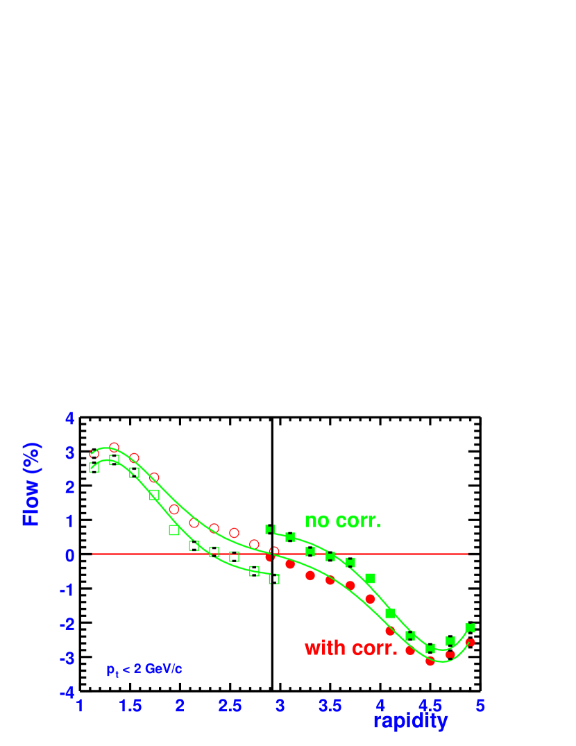
Figure 1: NA49 results on directed flow as a function of rapidity for charged pions from minimum bias 158$A$ GeV Pb + Pb. Shown are $v_{1}$ before (squares) and after (circles) correction for momentum conservation. Solid lines are polynomial fits. The open points have been reflected about midrapidity.

As an illustration, the method was applied to the NA49 data in Pb+Pb collisions at 158 GeV per nucleon Poskanzer:2001cx . In the analysis, the event plane was determined from charged pions with $p_{T}<1.0$ GeV/$c$, except for centrality bins 1 and 2, where the upper cuts were at 0.3 and 0.6 GeV/$c$, respectively. The $y$ values were between 4.0 and 6.0. The particles were assigned weights $w=|y-y_{\rm CM}|$, always positive since all used particles belong to the forward hemisphere. Then pions with known $p_{T}$ and $y$ values were correlated with this event plane (being careful to remove autocorrelations) to provide a matrix of observed $v_{1}(p_{T},y)$. The $\chi_{\rm sub}$ values were obtained from the correlation of subevent planes using Eqs. (23) and (27). In each $(p_{T},y)$ bin the momentum conservation correction was subtracted using Eq. (25). The full event plane resolution was obtained from Eq. (12) and, according to Eq. (17), the whole matrix was corrected for the event plane resolution to produce the double differential $v_{1}$ values. The procedure was done for each centrality bin separately and then the minimum bias results were produced by taking the weighted average over centrality, weighting with the cross section. The cross sections as a function of $p_{T}$, $y$, and centrality, had already been evaluated and parameterized crosssections . Figure 1 was produced by projecting this final matrix onto the rapidity axis, by taking the weighted average over $p_{T}$, again weighting with the cross section.

Table 1: Listed for the six centralities are: $N$, the total multiplicity over all phase space; $\left\langle p_{T}^{2}\right\rangle$, the mean $p_{t}^{2}$ over all phase space in units of GeV${}^{2}/c^{2}$; $M$, the multiplicity of particles used for the event plane; $f$, the fraction defined by Eq. (23); $\chi$, the resolution parameter for the full event plane; the resolution of the full event plane; and the percent increase in the resolution due to momentum conservation. The first two centralities had more restrictive $p_{T}$ cuts.

Centrality	1	2	3	4	5	6
$N$	2402	1971	1471	1028	717	457
$\left\langle p_{T}^{2}\right\rangle$, GeV${}^{2}/c^{2}$	0.32	0.32	0.31	0.30	0.28	0.27
$M$	135	184	152	108	75	46
$f$	0.07	0.14	0.17	0.17	0.17	0.17
$\chi$	0.20	0.25	0.39	0.45	0.48	0.47
resolution	0.18	0.22	0.33	0.38	0.40	0.39
res. increase, %	6.3	19.7	10.9	8.0	7.1	7.3

The parameterized cross sections were also used to derive the $\left\langle p_{T}^{2}\right\rangle$ for all particles in Eqs. (23) and (25). More specifically, in each centrality bin the average was obtained by taking 3/2 the sum of $p_{T}^{2}$ of the charged pions, plus twice the sum for the charged kaons, plus the fraction of nucleons which are thought to be participants, and then dividing by the total multiplicity. The values of the parameters used in this momentum conservation correction are shown in Table 1. The $\left\langle\sum p_{T}^{2}\right\rangle=N\left\langle p_{T}^{2}\right\rangle$ values range from 773 to 122 GeV${}^{2}/c^{2}$; a slightly higher value was used in Ref. Borghini:2000cm , resulting in a somewhat smaller correction. The last line of the table shows that the increase in resolution due to momentum conservation is always less than 20%.

However, Fig. 1 shows that the correction for the effect of momentum conservation on $v_{1}$ is indeed significant, roughly an absolute value of 1% in the whole rapidity range under study. The corrected correlation does give a directed flow vanishing at midrapidity within error bars, as it should. In fact, if one did not know $N$ and $\left\langle p_{T}^{2}\right\rangle$, one could force the data to go through zero at midrapidity as a way to evaluate this correction.

Appendix A Correlation between one particle and the event flow vector

In this Appendix, we compute the azimuthal correlation between a particle with momentum $p_{T}$ and the flow vector ${\bf Q}$ when both flow and momentum conservation are taken into account. Flow, which is defined as a correlation of outgoing momenta with the reaction plane, means here a correlation with the $x$-axis: the transverse momentum vector ${\bf p_{T}}$ in a given $y$ and $p_{T}$ window has a non-zero average value $\left\langle{\bf p_{T}}\right\rangle$ which is parallel to the $x$-axis, and the same holds for the flow vector ${\bf Q}$. If the only correlation was due to flow, we could write the normalized $N$-particle momentum distribution as a product of single-particle distributions:

$$\frac{dP}{d{\bf p_{T}}_{1}\cdots d{\bf p_{T}}_{N}}=F_{1}({\bf p_{T}}_{1})\cdots F_{N}({\bf p_{T}}_{N}),$$ (34)

where $N$ denotes the total number of outgoing particles. The $F_{j}({\bf p_{T}}_{j})$ are normalized to unity, and we further assume that they satisfy average momentum conservation $\left\langle{\bf p_{T}}_{1}+\cdots+{\bf p_{T}}_{N}\right\rangle=0$.

Here, we also take into account exact transverse momentum conservation, which is expressed by means of an additional Dirac constraint Borghini:2000cm :

$$\frac{dP}{d{\bf p_{T}}_{1}\cdots d{\bf p_{T}}_{N}}=\pi N\left\langle p_{T}^{2}\right\rangle F_{1}({\bf p_{T}}_{1})\cdots F_{N}({\bf p_{T}}_{N})\delta\left({\bf p_{T}}_{1}+\cdots+{\bf p_{T}}_{N}\right).$$ (35)

Note that $F_{j}({\bf p_{T}}_{j})$ no longer strictly represents the single-particle momentum distribution. The latter is now given by Borghini:2000cm :

$$\frac{dP}{d{\bf p_{T}}_{j}}=F_{j}({\bf p_{T}}_{j})\left(1-\frac{p_{Tj}^{2}-\left\langle p_{Tj}^{2}\right\rangle}{N\left\langle p_{T}^{2}\right\rangle}\right).$$ (36)

We are going to compute the correlated probability distribution between the transverse momentum of an arbitrary particle (which we choose to be the one labeled $N$, ${\bf p_{T}}_{N}$) and the flow vector ${\bf Q}$. To compute this probability distribution $dP/d{\bf p_{T}}_{N}d{\bf Q}$, we introduce the flow vector ${\bf Q}$ defined by Eq. (7) in Eq. (35) by means of a Dirac constraint, and integrate over the $N-1$ remaining particle momenta:

$$\frac{dP}{d{\bf p_{T}}_{N}d{\bf Q}}=\pi N\left\langle p_{T}^{2}\right\rangle F_{N}({\bf p_{T}}_{N})\int\!\left(\prod_{j=1}^{N-1}F_{j}({\bf p_{T}}_{j})d{\bf p_{T}}_{j}\right)\delta\left({\bf p_{T}}_{1}+\cdots+{\bf p_{T}}_{N}\right)\delta\left({\bf w}_{1}+\cdots+{\bf w}_{N}-{\bf Q}\right),$$ (37)

with ${\bf w}_{j}=w_{j}{\bf u}_{j}=(w_{j}/{p_{T}}_{j}){\bf p_{T}}_{j}$.

Using the Fourier representation of the Dirac distributions, this equation becomes

$$\frac{dP}{d{\bf p_{T}}_{N}d{\bf Q}}=\pi N\left\langle p_{T}^{2}\right\rangle F_{N}({\bf p_{T}}_{N})\int\!\frac{d^{2}{\bf k}}{(2\pi)^{2}}e^{i{\bf k}\cdot{\bf p_{T}}_{N}}\int\frac{d^{2}{\bf l}}{(2\pi)^{2}}e^{-i{\bf l}\cdot{\bf Q}}\prod_{j=1}^{N-1}\left(\int F_{j}({\bf p_{T}}_{j})e^{i({\bf k}\cdot{\bf p_{T}}_{j}+{\bf l}\cdot{\bf w}_{j})}d{\bf p_{T}}_{j}\right).$$ (38)

We have assumed that the particle with momentum ${\bf p_{T}}_{N}$ is not involved in the determination of the reaction plane, i.e., that ${\bf w}_{N}=0$, as one usually does to avoid autocorrelations Danielewicz:1985hn .

Since $N$ is large, the integrals over ${\bf k}$ and ${\bf l}$ can be evaluated by means of a saddle-point approximation, i.e., only small values of ${\bf k}$ and ${\bf l}$ contribute. Expanding to second order in ${\bf k}$ and ${\bf l}$ and re-exponentiating, one obtains

$$\int F({\bf p_{T}})e^{i({\bf k}\cdot{\bf p_{T}}+{\bf l}\cdot{\bf w})}d{\bf p_{T}}\simeq\exp\left(i{\bf k}\cdot\left\langle\bf p_{T}\right\rangle+i{\bf l}\cdot\left\langle\bf w\right\rangle-\frac{{\bf k}^{2}}{4}\left\langle p_{T}^{2}\right\rangle-\frac{{\bf l}^{2}}{4}\left\langle w^{2}\right\rangle-\frac{{\bf k}\cdot{\bf l}}{2}\left\langle wp_{T}\right\rangle\right),$$ (39)

where we have dropped the index $j$ for simplicity. In deriving this equation, we have assumed that directed flow is small for most particles, $|v_{1}|\ll 1$, so that terms of second order in the flow can be neglected, i.e. $\left\langle\bf p_{T}\right\rangle^{2}\ll\left\langle p_{T}^{2}\right\rangle$, etc. Note that the correlation between ${\bf p_{T}}_{N}$ and ${\bf Q}$ comes from the cross term, proportional to ${\bf k}\cdot{\bf l}$.

Inserting Eq. (39) into Eq. (38), the remaining integrals over ${\bf l}$ and ${\bf k}$ are Gaussian, and can thus be evaluated analytically. After some algebra, and dropping the index $N$ for sake of brevity, one finally obtains the result in the form

$$\displaystyle\frac{dP}{d{\bf p_{T}}d{\bf Q}}=\displaystyle\frac{dP}{d{\bf p_{T}}}\frac{dP}{d{\bf Q}}$$ (40)

$$\times\left(1+2\,c\left(\frac{{\bf p_{T}}-\left\langle\bf p_{T}\right\rangle}{p_{T}}\right)\cdot\left(\frac{{\bf Q}-\left\langle\bf Q\right\rangle}{\sigma}\right)\right).$$ (41)

In this equation, $dP/d{\bf p_{T}}$ denotes the single-particle momentum distribution [obtained by integrating Eq. (40) over ${\bf Q}$], given by Eq. (36), and $dP/d{\bf Q}$ the distribution of the flow vector ${\bf Q}$ [obtained by integrating Eq. (40) over ${\bf p_{T}}$], given by Eq. (11). The dimensionless correlation strength $c$ is given by

$$c\equiv-\frac{p_{T}}{\sqrt{N\left\langle p_{T}^{2}\right\rangle}}\,\frac{f}{\sqrt{1-f^{2}}},$$ (42)

where $f$ is given by Eq. (23). Finally, the width of the distribution of ${\bf Q}$ is

$$\sigma^{2}\equiv N\,\left\langle w^{2}\right\rangle\left(1-f^{2}\right).$$ (43)

In this expression, $(1-f^{2})$ is the correction to the width due to momentum conservation.

The above expressions of $c$ and $\sigma$ have been obtained by a “brute force” calculation, but one can easily recover them directly from the distribution (40), and the correlation due to momentum conservation, Eq. (6), which we rewrite in the form

$$\left\langle{\bf u_{1}}\cdot{\bf u_{2}}\right\rangle-\left\langle{\bf u_{1}}\right\rangle\cdot\left\langle{\bf u_{2}}\right\rangle=-\frac{{p_{T}}_{1}{p_{T}}_{2}}{N\left\langle p_{T}^{2}\right\rangle}.$$ (44)

From the distribution of ${\bf Q}$, Eq. (11), one obtains $\sigma^{2}=\left\langle{\bf Q}^{2}\right\rangle-\left\langle\bf Q\right\rangle^{2}$. Using the definition of ${\bf Q}$, Eq. (7), and Eq. (44), it is a simple exercise to check Eq. (43). Similarly, Eq. (40) allows to express the correlation strength $c$ in terms of simple averages: $c=(\left\langle{\bf p_{T}}\cdot{\bf Q}\right\rangle-\left\langle\bf p_{T}\right\rangle\cdot\left\langle\bf Q\right\rangle)/(\sigma p_{T})$, which can also be easily calculated using Eqs. (7) and (44).

As explained in Sec.IV, there are two ways of eliminating the correlation in Eq. (40). The first possibility is to shift the flow vector for each particle. Making the change of variables ${\bf Q^{\prime}}={\bf Q}-c\sigma{\bf p_{T}}/p_{T}$ in the distribution Eqs. (11) and expanding to first order in the correlation $c$, one easily checks that the correlated term in Eq. (40) cancels, so that the distributions of ${\bf Q^{\prime}}$ and ${\bf p_{T}}$ are uncorrelated. Replacing $c$ and $\sigma$ by their expressions (43) and (42), one recovers Eq. (19).

Instead of redefining the flow vector, one can compute the azimuthal correlation between the particle and the flow vector using the correlated distribution Eq. (40). The first term in the right-hand side gives the correlation due to flow, while the second term corresponds to the correlation due to momentum conservation, that is, the term we wish to calculate. This term gives the following contribution:

$$\left\langle\cos(\phi-\Phi)\right\rangle_{\rm mom.\ cons.}=\frac{c}{\sigma}\left(\left\langle Q\right\rangle-\left\langle\cos\Delta\Phi\right\rangle{\bf e}_{x}\cdot\left\langle\bf Q\right\rangle\right),$$ (45)

The resolution $\left\langle\cos\Delta\Phi\right\rangle$ is given by Eq. (12), and $\left\langle Q\right\rangle$ is obtained by a similar calculation from the Gaussian distribution (11):

$$\left\langle Q\right\rangle=\sigma\,\frac{\sqrt{\pi}}{2}\,e^{-\chi^{2}/2}\left[(1+\chi^{2})I_{0}(\chi^{2}/2)+\chi^{2}I_{1}(\chi^{2}/2)\right].$$ (46)

The terms proportional to $I_{1}(\chi^{2}/2)$ cancel, and one finally obtains

$$\left\langle\cos(\phi-\Phi)\right\rangle_{\rm mom.\ cons.}=c\,\frac{\sqrt{\pi}}{2}e^{-\chi^{2}/2}I_{0}(\chi^{2}/2).$$ (47)

In the limit $\chi\ll 1$ (poor resolution), this equals approximately $c\sqrt{\pi}/2$, while for $\chi\gg 1$ (good resolution), the correction decreases like $c/(2\chi)$.

Appendix B Correlation between two subevents

We shall now compute the azimuthal correlation between two subevents, which we denote ${\bf Q_{a}}$ and ${\bf Q_{b}}$, in the presence of flow and momentum conservation. For simplicity, we assume throughout the following discussion that both subevents are equivalent, and moreover that they are of equal multiplicities. Since both contain a large number of particles, we may directly apply the central limit theorem. The normalized correlated distribution is thus Gaussian:

$$\frac{dP}{d{\bf Q_{a}}d{\bf Q_{b}}}=\frac{1}{\pi^{2}\sigma_{a}^{4}(1-C^{2})}\exp\left(-\frac{({\bf Q_{a}}-\left\langle\bf Q_{a}\right\rangle)^{2}+({\bf Q_{b}}-\left\langle\bf Q_{b}\right\rangle)^{2}-2C({\bf Q_{a}}-\left\langle\bf Q_{a}\right\rangle)\cdot({\bf Q_{b}}-\left\langle\bf Q_{b}\right\rangle)}{\sigma_{a}^{2}(1-C^{2})}\right).$$ (48)

In this equation, $C$ represents the strength of the “nonflow” correlation (in particular, that due to momentum conservation) between the subevents. For $C=0$, subevents are independent, and the distribution (48) factorizes into the product of two distributions of the type (13). In the more general case $C\not=0$, one recovers Eq. (13) by integrating Eq. (48) over ${\bf Q_{b}}$.

When correlations due to momentum conservation are taken into account, the width $\sigma_{\rm sub}^{2}=\left\langle{\bf Q_{\rm sub}}^{2}\right\rangle-\left\langle\bf Q_{\rm sub}\right\rangle^{2}$ is given by a formula analogous to Eq. (43), with the important difference that $N$ and $f^{2}$ are replaced by $N/2$ and $f^{2}/2$, since we use only half the particles to construct the subevents:

$$\sigma_{\rm sub}^{2}\equiv\frac{N}{2}\,\left\langle w^{2}\right\rangle\left(1-\frac{f^{2}}{2}\right).$$ (49)

Note that $\sigma_{\rm sub}$ is not simply equal to $\sigma/\sqrt{2}$, because of the term arising from correlations.

Let us now calculate the correlation strength $C$. It can be obtained by taking the following average value with the probability distribution (48) Poskanzer:1998yz ; Ollitrault:dy :

$$C = \frac{\left\langle({\bf Q_{a}}-\left\langle\bf Q_{a}\right\rangle)\cdot({\bf Q_{b}}-\left\langle\bf Q_{b}\right\rangle)\right\rangle}{\sigma_{a}^{2}}$$ (50)

$$= \frac{\left\langle{\bf Q_{a}}\cdot{\bf Q_{b}}\right\rangle-\left\langle\bf Q_{a}\right\rangle\cdot\left\langle\bf Q_{b}\right\rangle}{\sigma_{a}^{2}}.$$ (51)

Using the definitions of ${\bf Q_{a}}$ and ${\bf Q_{b}}$ and the correlation from momentum conservation, Eq. (44), the numerator of Eq. (50) is equal to $-(N/2)^{2}\left\langle wp_{T}\right\rangle^{2}/N\left\langle p_{T}^{2}\right\rangle$, where we have neglected terms of second order in flow. With the width given by Eq. (49), we finally obtain

$$C=\frac{-\left\langle wp_{T}\right\rangle^{2}}{2\left\langle p_{T}^{2}\right\rangle\left\langle w^{2}\right\rangle(1-f^{2}/2)}=\frac{-f^{2}}{2-f^{2}},$$ (52)

where $f$ is given by Eq. (23).

As explained in Sec. III, the resolution parameter $\chi_{\rm sub}=\langle{\bf Q_{\rm sub}}\rangle\cdot{\bf e_{x}}/\sigma_{\rm sub}$ of the subevent is obtained from the distribution of the relative angle between ${\bf Q_{a}}$ and ${\bf Q_{b}}$. Unfortunately, there is no general analytic expression for this distribution.

Useful expressions can be obtained in a few limiting cases. First, if the correlation strength $C$ is much smaller than unity, the distribution (48) can be expanded to first order in $C$, which yields a distribution analogous to Eq. (40). From this expression, one can in particular evaluate the average cosine $\left\langle\cos(\Phi_{a}-\Phi_{b})\right\rangle$, which leads to Eq. (27). Second, if the resolution is high ($\chi_{\rm sub}\gg 1$), both ${\bf Q_{a}}$ and ${\bf Q_{b}}$ are close to their average value $\left\langle\bf Q_{\rm sub}\right\rangle$, so that their azimuthal angles with respect to the reaction plane are small, and one may approximate $\Phi_{a}\simeq{\bf Q_{a}}\cdot{\bf e_{y}}/|\left\langle\bf Q_{a}\right\rangle|$, and a similar expression for $\Phi_{b}$. In this limiting case, the distribution of $\Phi_{a}$ and $\Phi_{b}$ is a Gaussian, and the distribution of the relative angle is given by Eq. (31).

Quite remarkably, one can derive an exact expression, valid for arbitrary $\chi_{\rm sub}$ and $C$, of the fraction of events for which the angle between subevents is larger than $\pi/2$, taking into account both flow and momentum conservation. The condition $|\Phi_{a}-\Phi_{b}|>\pi/2$ can equivalently be written ${\bf Q_{a}}\cdot{\bf Q_{b}}<0$, so that

$$P(|\Phi_{a}-\Phi_{b}|>\pi/2)=\int{d{\bf Q_{a}}d{\bf Q_{b}}\frac{dP}{d{\bf Q_{a}}d{\bf Q_{b}}}\,\theta(-{\bf Q_{a}}\cdot{\bf Q_{b}})}.$$ (53)

We then insert the Fourier representation of Heaviside’s step function $\theta(x)$:

$$\theta(-x)=\frac{i}{2\pi}\lim_{\varepsilon\to 0^{+}}\int_{-\infty}^{+\infty}\frac{e^{2ikx}}{k+i\varepsilon}dk.$$ (54)

With the probability distribution Eq. (48), the integrals on ${\bf Q_{a}}$ and ${\bf Q_{b}}$ are Gaussian and can be evaluated analytically. One obtains

$$P(|\Phi_{a}-\Phi_{b}|>\pi/2)=\frac{i}{2\pi}\int_{-\infty}^{+\infty}\frac{dk}{(k+i\varepsilon)\left[1-ik(1+C)\right]\left[1+ik(1-C)\right]}\exp\left[\frac{2i\chi^{2}k}{1-ik(1+C)}\right]$$ (55)

The only essential singularity of the integrand occurs in the lower half plane at $k=-i/(1+C)$. Therefore the integral can be calculated by closing the contour on the upper half plane. The only pole is at $k=i/(1-C)$, and the theorem of residues yields Ollitrault:dy

$$P(|\Phi_{a}-\Phi_{b}|>\pi/2)=\frac{1-C}{2}e^{-\chi_{\rm sub}^{2}}.$$ (56)

Inserting the correlation strength Eq. (52) in this expression, one recovers Eq. (30).

References

- (1) S. Voloshin and Y. Zhang, Z. Phys. C 70, 665 (1996) [hep-ph/9407282].
- (2) P. Danielewicz and G. Odyniec, Phys. Lett. B 157, 146 (1985).
- (3) D. J. Magestro, W. Bauer, and G. D. Westfall, Phys. Rev. C 62, 041603 (2000).
- (4) P. Danielewicz et al., Phys. Rev. C 38, 120 (1988).
- (5) C. A. Ogilvie et al., Phys. Rev. C 40, 2592 (1989).
- (6) D. Cussol et al. [INDRA Collaboration], Phys. Rev. C 65, 044604 (2002) [nucl-ex/0111007].
- (7) E. P. Prendergast et al., Phys. Rev. C 61, 024611 (2000).
- (8) P. Crochet et al. [FOPI Collaboration], Nucl. Phys. A 624, 755 (1997) [nucl-ex/9707007]; F. Rami et al. [FOPI Collaboration], ibid. 646, 367 (1999) [nucl-ex/9812005].
- (9) L. Ahle et al. [E802 Collaboration], Phys. Rev. C 57, 1416 (1998).
- (10) H. Liu et al. [E895 Collaboration], Phys. Rev. Lett. 84, 5488 (2000) [nucl-ex/0005005]; P. Chung et al. [E895 Collaboration], ibid. 85, 940 (2000) [nucl-ex/0101003]; ibid. 86, 2533 (2001) [nucl-ex/0101002].
- (11) Q. B. Pan and P. Danielewicz, Phys. Rev. Lett. 70, 2062 (1993) [Erratum-ibid. 70, 3523 (1993)].
- (12) B. A. Li, C. M. Ko, and G. Q. Li, Phys. Rev. C 54, 844 (1996) [nucl-th/9605014].
- (13) B. A. Li and A. T. Sustich, Phys. Rev. Lett. 82, 5004 (1999) [nucl-th/9905038].
- (14) B. A. Li, Phys. Rev. Lett. 85, 4221 (2000) [nucl-th/ 0009069].
- (15) P. Crochet et al. [FOPI Collaboration], Phys. Lett. B 486, 6 (2000) [nucl-ex/0006004]; A. Andronic et al. [FOPI Collaboration], Phys. Rev. C 64, 041604 (2001) [nucl-ex/0108014].
- (16) J. Barrette et al. [E877 Collaboration], Phys. Rev. C 56, 3254 (1997) [nucl-ex/9707002]; ibid. 59, 884 (1999) [nucl-ex/9805006]; Phys. Lett. B 485, 319 (2000) [nucl-ex/0004002]; Phys. Rev. C 63, 014902 (2001) [nucl-ex/0007007].
- (17) H. Appelshäuser et al. [NA49 Collaboration], Phys. Rev. Lett. 80, 4136 (1998) [nucl-ex/9711001, http:// na49info.cern.ch/na49/Archives/Images/Publications/ Phys.Rev.Lett.80:4136-4140,1998/]; A. M. Poskanzer, Nucl. Phys. A638 463c (1998); A. M. Poskanzer and S. A. Voloshin, ibid. A661, 341c (1999) [nucl-ex/ 9906013].
- (18) N. Borghini, P. M. Dinh, and J.-Y. Ollitrault, Phys. Rev. C 62, 034902 (2000) [nucl-th/0004026].
- (19) S. Wang et al., Phys. Rev. C 44, 1091 (1991).
- (20) A. M. Poskanzer and S. A. Voloshin, Phys. Rev. C 58, 1671 (1998) [nucl-ex/9805001].
- (21) R. A. Lacey [PHENIX Collaboration], Nucl. Phys. A 698, 559c (2002) [nucl-ex/0105003].
- (22) J.-Y. Ollitrault, Phys. Rev. D 46, 229 (1992).
- (23) J.-Y. Ollitrault, nucl-ex/9711003.
- (24) J.-Y. Ollitrault, Phys. Rev. D 48, 1132 (1993) [hep-ph/9303247].
- (25) A. Taranenko et al. [TAPS Collaboration], nucl-ex/ 9910002.
- (26) A. Andronic et al. [FOPI Collaboration], Nucl. Phys. A 679, 765 (2001) [nucl-ex/0008007]; L. Simić and J. Milošević, J. Phys. G 27, 183 (2001) [nucl-th/0106037]; C. Pinkenburg et al. [E895 Collaboration], Phys. Rev. Lett. 83, 1295 (1999) [nucl-ex/9903010]; P. Chung et al. [E895 Collaboration], nucl-ex/0112002.
- (27) J.-Y. Ollitrault, Nucl. Phys. A 590, 561c (1995).
- (28) Y. Dai [E877 Collaboration], PhD thesis, McGill University, Montréal, Canada, 1998 [http://www-aix.gsi.de/ misko/e877/theses/theses.html].
- (29) K. H. Ackermann et al. [STAR Collaboration], Phys. Rev. Lett. 86, 402 (2001) [nucl-ex/0009011].
- (30) P. M. Dinh, N. Borghini, and J.-Y. Ollitrault, Phys. Lett. B 477, 51 (2000) [nucl-th/9912013].
- (31) N. Borghini, P. M. Dinh, and J.-Y. Ollitrault, Phys. Rev. C 64, 054901 (2001) [nucl-th/0105040].
- (32) A. M. Poskanzer, nucl-ex/0110013.
- (33) G. E. Cooper, PhD thesis, University of California at Berkeley, 2000 [LBNL-45467, http://na49info.cern.ch/ cgi-bin/wwwd-util/NA49/NOTE?222].