Nucleon mass and pion loops

Abstract

Poincaré covariant Faddeev equations for the nucleon and $\Delta$ are solved to illustrate that an internally consistent description in terms of confined-quark and nonpointlike confined-diquark-correlations can be obtained. $\pi N$-loop induced self-energy corrections to the nucleon’s mass are analysed and shown to be independent of whether a pseudoscalar or pseudovector coupling is used. Phenomenological constraints suggest that this self-energy correction reduces the nucleon’s mass by up to several hundred MeV. That effect does not qualitatively alter the picture, suggested by the Faddeev equation, that baryons are quark-diquark composites. However, neglecting the $\pi$-loops leads to a quantitative overestimate of the nucleon’s axial-vector diquark component.

I Introduction

Contemporary experimental facilities employ large momentum transfer reactions to probe the structure of hadrons and thereby attempt to elucidate the role played by quarks and gluons in building them. Since the proton is a readily accessible target its properties have been studied most extensively Thomas:kw . Hence an understanding of a large fraction of the available data requires a Poincaré covariant theoretical description of the nucleon.

At its simplest the nucleon is a nonperturbative three-body bound-state problem, an exact solution of which is difficult to obtain even if the interactions are known. Hitherto, therefore, phenomenological mean-field models have been widely employed to describe nucleon structure; e.g., soliton models wilets ; Birse:cx ; reinhardTS and constituent-quark models tonyCBM ; tonyANU ; simon . These models are most naturally applied to processes involving small momentum transfer ($q^{2}<M^{2}$, $M$ is the nucleon mass) and, as commonly formulated, their applicability may be extended to processes involving larger momentum transfer by working in the Breit frame gerrytony . Alternatively, one could define an equivalent, Galilean invariant Hamiltonian and reinterpret that as the Poincaré invariant mass operator for a quantum mechanical theory fritz but this path is less well travelled.

Another approach is to describe the nucleon via a Poincaré covariant Faddeev equation. That, too, requires an assumption about the interaction between quarks. An analysis regbos of the Global Colour Model gcm ; petergcm ; gunnergcm suggests that the nucleon can be viewed as a quark-diquark composite. Pursuing that picture yields regfe a Faddeev equation, in which two quarks are always correlated as a colour-antitriplet diquark quasiparticle (because ladder-like gluon exchange is attractive in the $\bar{3}_{c}$ quark-quark scattering channel) and binding in the nucleon is effected by the iterated exchange of roles between the dormant and diquark-participant quarks.

A first numerical study of this Faddeev equation for the nucleon was reported in Ref. cjbfe , and following that there have been numerous more extensive analyses; e.g., Refs. bentz ; oettel . In particular, the formulation of Ref. oettel employs confined quarks, and confined, pointlike-scalar and -axial-vector diquark correlations, to obtain a spectrum of octet and decuplet baryons in which the rms-deviation between the calculated mass and experiment is only $2$%. The model also reproduces nucleon form factors over a large range of momentum transfer oettel2 , and its descriptive success in that application is typical of such Poincaré covariant treatments; e.g., Refs. jacquesA ; jacquesmyriad ; cdrqciv ; nedm .

However, these successes might themselves indicate a flaw in the application of the Faddeev equation to the nucleon. For example, in the context of spectroscopy, studies using the Cloudy Bag Model (CBM)  tonyCBM indicate that the dressed-nucleon’s mass receives a negative contribution of as much as $300$-$400\,$MeV from pion self-energy corrections; i.e., $\delta M_{+}=-300\,$ to $-400\,$MeV tonyANU ; bruceCBM . Furthermore, a perturbative study, using the Faddeev equation, of the mass shift induced by pointlike-$\pi$ exchange between the quark and diquark constituents of the nucleon obtains $\delta M_{+}=-150$ to $-300\,$MeV ishii . Unameliorated these mutually consistent results would much diminish the value of the $2$% spectroscopic accuracy obtained using only quark and diquark degrees of freedom.

It is thus apparent that the size and qualitative impact of the pionic contribution to the nucleon’s mass may provide material constraints on the development of a realistic quark-diquark picture of the nucleon, and its interpretation and application. Our article is an exploration of this possibility and we aim to clarify the model dependent aspects. We emphasise, in addition, that chiral corrections to baryon magnetic moments and charge radii are also important radiiCh , and their model-independent features furnish additional constraints on any quark model, including those based on the Faddeev equation, thereby guiding their improvement. We note, too, that lattice-QCD studies of baryon masses, especially as a function of the current-quark mass LQCD , also provide information that can guide these considerations; e.g., a recent lattice-QCD exploration of the connection between $N$ and $\Delta$ masses is consistent with the pion self-energies described above Young:2001nc .

In Sec. II we recapitulate on the Faddeev equation and its solution for the $N$ and $\Delta$ in a simple model. Section III discusses model-independent aspects of the Dyson-Schwinger equation (DSE) cdragw that describes the pionic correction to the $N$’s self-energy and therein we also present exemplary estimates for the magnitude of the effect. Section IV is an epilogue.

II Faddeev Equation

The properties of light pseudoscalar and vector mesons are well described by a renormalisation-group-improved rainbow-ladder truncation of QCD’s DSEs mr97 ; pieterrho ; pieterGamma , and the study of baryons via the solution of a Poincaré covariant Faddeev equation is a desirable extension of the approach. The derivation of a Faddeev equation for the bound state contribution to the three quark scattering kernel is possible because the same kernel that describes mesons so well is also strongly attractive for quark-quark scattering in the colour-antitriplet channel (see Sec. II.1.2). And it is a simple consequence of the Clebsch-Gordon series for quarks in the fundamental representation of $SU_{c}(3)$:

$$3_{c}\otimes 3_{c}\otimes 3_{c}=(\bar{3}_{c}\oplus 6_{c})\otimes 3_{c}=1_{c}\oplus 8_{c}^{\prime}\oplus 8_{c}\oplus 10_{c}\,,$$ (1)

that any two quarks in a colour singlet bound state must constitute a relative colour antitriplet. This supports a truncation of the three-body problem wherein the interactions between two selected quarks are added to yield a quark-quark scattering matrix, which is then approximated as a sum over all possible diquark pseudoparticle terms: Dirac-scalar $+$ -pseudovector $+[\ldots]$ – essentially a separable two-body interaction Modern . A Faddeev equation follows, which describes the three-body bound-state as a composite of a dressed-quark and nonpointlike diquark with an iterated exchange of roles between the dormant and diquark-participant quarks. The bound-state is represented by a Faddeev amplitude:

$$\Psi=\Psi_{1}+\Psi_{2}+\Psi_{3}\,,$$ (2)

where the subscript identifies the dormant quark and, e.g., $\Psi_{1,2}$ are obtained from $\Psi_{3}$ by a correlated, cyclic permutation of all the quark labels.

The Faddeev equation is simplified further by retaining only the lightest diquark correlations in the representation of the quark-quark scattering matrix. A simple, Goldstone-theorem-preserving, rainbow-ladder DSE-model conradsep yields the following diquark pseudoparticle masses (isospin symmetry is assumed):

$$\begin{array}[]{l|cccc}(qq)_{J^{P}}&(ud)_{0^{+}}&(us)_{0^{+}}&(uu)_{1^{+}}&(us)_{1^{+}}\\ m_{qq}\,({\rm GeV})&0.74&0.88&0.95&1.05\\ \hline\cr(qq)_{J^{P}}&(ss)_{1^{+}}&(uu)_{1^{-}}&(us)_{1^{-}}&(ss)_{1^{-}}\\ m_{qq}\,({\rm GeV})&1.13&1.47&1.53&1.64\end{array}$$ (3)

The mass ordering is characteristic and model-independent (cf. Refs. gunner ; pieterdq , lattice-QCD estimates latticediquark and studies of the spin-flavour dependence of parton distributions Close:br ), and indicates that a study of the $N$ and $\Delta$ must retain at least the scalar and pseudovector $(uu)$- and $(ud)$-correlations if it is to be accurate. (Of course, the spin-$3/2$ $\Delta$ is inaccessible unless pseudovector correlations are retained.)

II.1 Model for the Nucleon

To provide a concrete illustration and make our presentation self-contained we consider a simple model cdrqciv wherein the nucleon is a sum of scalar and pseudovector diquark correlations:

$$\Psi_{3}(p_{i},\alpha_{i},\tau_{i})=\Psi_{3}^{0^{+}}+\Psi_{3}^{1^{+}},$$ (4)

with $(p_{i},\alpha_{i},\tau_{i})$ the momentum, spin and isospin labels of the quarks constituting the nucleon, and $P=p_{1}+p_{2}+p_{3}$ the nucleon’s total momentum. The scalar diquark component in Eq. (4) is

$$\Psi_{3}^{0^{+}}(p_{i},\alpha_{i},\tau_{i})=$$

$$[\Gamma^{0^{+}}(\frac{1}{2}p_{[12]};K)]_{\alpha_{1}\alpha_{2}}^{\tau_{1}\tau_{2}}\,\Delta^{0^{+}}(K)\,[{\cal S}(\ell;P)u(P)]_{\alpha_{3}}^{\tau_{3}}\,,$$

where fn:Euclidean : the spinor satisfies

$$(i\gamma\cdot P+M)\,u(P)=0=\bar{u}(P)\,(i\gamma\cdot P+M)\,,$$ (6)

with $M$ the mass obtained in solving the Faddeev equation, and is also a spinor in isospin space with $\varphi_{+}={\rm col}(1,0)$ for the proton and $\varphi_{-}={\rm col}(0,1)$ for the neutron; $K=p_{1}+p_{2}=:p_{\{12\}}$, $p_{[12]}=p_{1}-p_{2}$, $\ell:=(-p_{\{12\}}+2p_{3})/3$; $\Delta^{0^{+}}(K)$ is a pseudoparticle propagator for the scalar diquark formed from quarks $1$ and $2$, and $\Gamma^{0^{+}}\!$ is a Bethe-Salpeter-like amplitude describing their relative momentum correlation; and ${\cal S}$, a $4\times 4$ Dirac matrix, describes the relative quark-diquark momentum correlation. (${\cal S}$, $\Gamma^{0^{+}}$ and $\Delta^{0^{+}}$ are discussed below.) The pseudovector component is

$$\Psi^{1^{+}}(p_{i},\alpha_{i},\tau_{i})=$$

$$[{\tt t}^{i}\,\Gamma_{\mu}^{1^{+}}(\frac{1}{2}p_{[12]};K)]_{\alpha_{1}\alpha_{2}}^{\tau_{1}\tau_{2}}\,\Delta_{\mu\nu}^{1^{+}}(K)\,[{\cal A}^{i}_{\nu}(\ell;P)u(P)]_{\alpha_{3}}^{\tau_{3}}\,,$$

where the symmetric isospin-triplet matrices are

$${\tt t}^{+}=\frac{1}{\surd 2}(\tau^{0}+\tau^{3})\,,\;{\tt t}^{0}=\tau^{1}\,,\;{\tt t}^{-}=\frac{1}{\surd 2}(\tau^{0}-\tau^{3})\,,$$ (8)

with $(\tau^{0})_{ij}=\delta_{ij}$ and $\tau^{1,3}$ the usual Pauli matrices, and the other elements in Eq. (LABEL:calA) are obvious generalisations of those in Eq. (LABEL:calS).

The colour antisymmetry of $\Psi_{3}$ is implicit in $\Gamma^{J^{P}}\!$, with the Levi-Civita tensor, $\epsilon_{c_{1}c_{2}c_{3}}$, expressed via the antisymmetric Gell-Mann matrices; i.e., defining

$$\{H^{1}=i\lambda^{7},H^{2}=-i\lambda^{5},H^{3}=i\lambda^{2}\}\,,$$ (9)

then $\epsilon_{c_{1}c_{2}c_{3}}=(H^{c_{3}})_{c_{1}c_{2}}$. (See Eqs. (37), (38).)

The Faddeev equation satisfied by $\Psi_{3}$ yields a set of coupled equations for the matrix valued functions ${\cal S}$, ${\cal A}_{\nu}^{i}$:

$$\left[\begin{array}[]{r}{\cal S}(k;P)\,u(P)\\ {\cal A}^{i}_{\mu}(k;P)\,u(P)\end{array}\right]$$ (15)

$$=-4\,\int\frac{d^{4}\ell}{(2\pi)^{4}}\,{\cal M}(k,\ell;P)\left[\begin{array}[]{r}{\cal S}(\ell;P)\,u(P)\\ {\cal A}^{j}_{\nu}(\ell;P)\,u(P)\end{array}\right],$$

where one factor of “2” appears because $\Psi_{3}$ is coupled symmetrically to $\Psi_{1}$ and $\Psi_{2}$, and we have evaluated the necessary colour contraction: $(H^{a})_{bc}(H^{a})_{cb^{\prime}}=-2\,\delta_{bb^{\prime}}$.

The kernel in Eq. (15) is

$${\cal M}(k,\ell;P)=\left[\begin{array}[]{cc}{\cal M}_{00}&({\cal M}_{01})^{j}_{\nu}\\ ({\cal M}_{10})^{i}_{\mu}&({\cal M}_{11})^{ij}_{\mu\nu}\rule{0.0pt}{12.91663pt}\end{array}\right]$$ (16)

with

$${\cal M}_{00}=\Gamma^{0^{+}}(k_{q}-\ell_{qq}/2;\ell_{qq})\,S^{\rm T}(\ell_{qq}-k_{q})\,$$ (17)

$$\times\,\bar{\Gamma}^{0^{+}}(\ell_{q}-k_{qq}/2;-k_{qq})\,S(\ell_{q})\,\Delta^{0^{+}}(\ell_{qq})\,,$$

where: $\ell_{q}=\ell+P/3$, $k_{q}=k+P/3$, $\ell_{qq}=-\ell+2P/3$, $k_{qq}=-k+2P/3$; $S$ is the propagator of the dormant dressed-quark constituent of the nucleon (Sec. II.1.1); and

$$({\cal M}_{01})^{j}_{\nu}={\tt t}^{j}\,\Gamma_{\mu}^{1^{+}}(k_{q}-\ell_{qq}/2;\ell_{qq})\,S^{\rm T}(\ell_{qq}-k_{q})\,$$ (18)

$$\times\,\bar{\Gamma}^{0^{+}}(\ell_{q}-k_{qq}/2;-k_{qq})\,S(\ell_{q})\,\Delta^{1^{+}}_{\mu\nu}(\ell_{qq})\,,$$

$$({\cal M}_{10})^{i}_{\mu}=\Gamma^{0^{+}}(k_{q}-\ell_{qq}/2;\ell_{qq})\,S^{\rm T}(\ell_{qq}-k_{q})\,$$ (19)

$$\times\,{\tt t}^{i}\,\bar{\Gamma}_{\mu}^{1^{+}}(\ell_{q}-k_{qq}/2;-k_{qq})\,S(\ell_{q})\,\Delta^{0^{+}}(\ell_{qq})\,,$$

$$({\cal M}_{11})^{ij}_{\mu\nu}={\tt t}^{j}\,\Gamma_{\rho}^{1^{+}}(k_{q}-\ell_{qq}/2;\ell_{qq})\,S^{\rm T}(\ell_{qq}-k_{q})\,$$ (20)

$$\times\,{\tt t}^{i}\,\bar{\Gamma}^{1^{+}}_{\mu}(\ell_{q}-k_{qq}/2;-k_{qq})\,S(\ell_{q})\,\Delta^{1^{+}}_{\rho\nu}(\ell_{qq})\,.$$

In Eqs. (15)-(20) it is implicit that $u(P)$ is a normalised average of $\varphi_{\pm}$ so that, e.g., the equation for the proton is obtained by projection on the left with $\varphi^{\dagger}_{+}$. To clarify this, by illustration, we note that Eq. (19) generates an isospin coupling between $u(P)_{\varphi_{+}}$ on the l.h.s. of Eq. (15) and, on the r.h.s.,

$$\surd 2\,{\cal A}^{+}_{\nu}\,u(P)_{\varphi^{-}}-{\cal A}^{0}_{\nu}\,u(P)_{\varphi_{+}}\,.$$ (21)

This is merely the Clebsch-Gordon coupling of isospin-$1\oplus\,$isospin-$\frac{1}{2}$ to total isospin-$\frac{1}{2}$ and means that the scalar diquark amplitude in the proton, $(ud)_{0^{+}}\,u$, is coupled to itself and the linear combination:

$$\surd 2\,(uu)_{1^{+}}\,d-(ud)_{1^{+}}\,u\,.$$ (22)

The general forms of ${\cal S}$ and ${\cal A}_{\mu}^{i}$, the Bethe-Salpeter-like amplitudes that describe the momentum-space correlation between the quark and diquark in the nucleon, are discussed at length in Ref. oettel , wherein a detailed analysis of the Faddeev equation’s solution is presented. Requiring that ${\cal S}$ be an eigenfunction of $\Lambda_{+}(P)$, Eq. (132), entails

$${\cal S}(\ell;P)=f_{1}(\ell;P)\,I_{\rm D}+\frac{1}{M}\left(i\gamma\cdot\ell-\ell\cdot\hat{P}\,I_{\rm D}\right)\,f_{2}(\ell;P)\,,$$ (23)

where $(I_{\rm D})_{rs}=\delta_{rs}$, $\hat{P}^{2}=-1$, and, in the nucleon rest frame, $f_{1,2}$ describe, respectively the upper, lower component of the bound-state nucleon’s spinor. Requiring the same of ${\cal A}^{i}_{\mu}$ reduces to only six (from an original twelve) the number of independent Dirac amplitudes required to specify it completely. However, we simplify this by retaining only those two amplitudes that survive in the non-relativistic limit:

$${\cal A}_{\mu}^{i}(\ell;P)=a_{1}^{i}(\ell;P)\,\gamma_{5}\gamma_{\mu}+a_{2}^{i}(\ell;P)\,\gamma_{5}\gamma\cdot\hat{\ell}\,\hat{\ell}_{\mu}\,,\;\hat{\ell}^{2}=1.$$ (24)

Assuming isospin symmetry then: $a_{j}^{1}=a_{j}^{2}=a_{j}^{3}$, $j=1,2$.

The Faddeev equation for the nucleon is Eq. (15) with the kernel, ${\cal M}$, given by Eqs. (16)-(20): to complete its definition we must specify the dressed-quark propagator, the diquark Bethe-Salpeter amplitudes and the diquark propagators.

II.1.1 Dressed-quarks

The general form of the dressed-quark propagator is

$$S(p) = -i\gamma\cdot p\,\sigma_{V}(p^{2})+\sigma_{S}(p^{2})\,,$$ (25)

$$= [i\gamma\cdot p\,A(p^{2})+B(p^{2})]^{-1}\,.$$ (26)

It can be obtained by solving the QCD gap equation; i.e., the DSE for the dressed-quark self energy, and the many such studies cdragw ; revbasti ; revreinhard yield the model-independent result that the wave function renormalisation and dressed-quark mass:

$$Z(p^{2})=1/A(p^{2})\,,\;M(p^{2})=B(p^{2})/A(p^{2})\,,$$ (27)

respectively, exhibit significant momentum dependence for $p^{2}\lesssim 1\,$GeV², which is nonperturbative in origin. This behaviour was recently observed in lattice-QCD simulations latticequark , and Refs. pmqciv ; tandyadelaide provide quantitative comparisons between those results and a modern DSE model. The infrared enhancement of $M(p^{2})$ is an essential consequence of dynamical chiral symmetry breaking (DCSB) and is the origin of the constituent-quark mass. With increasing $p^{2}$ the mass function evolves to reproduce the asymptotic behaviour familiar from perturbative analyses, and that behaviour is unambiguously evident for $p^{2}\gtrsim 10\,$GeV² mr97 .

While numerical solutions of the quark DSE are readily obtained, the utility of an algebraic form for $S(p)$ is self-evident. An efficacious parametrisation of $S(p)$, which exhibits the features described above, has been used extensively in studies of meson properties revbasti ; revreinhard and we use it herein. It is expressed via

$$\bar{\sigma}_{S}(x) = 2\,\bar{m}\,{\cal F}(2(x+\bar{m}^{2}))$$ (28)

$$+{\cal F}(b_{1}x)\,{\cal F}(b_{3}x)\,\left[b_{0}+b_{2}{\cal F}(\epsilon x)\right]\,,$$

$$\bar{\sigma}_{V}(x) = \frac{1}{x+\bar{m}^{2}}\,\left[1-{\cal F}(2(x+\bar{m}^{2}))\right]\,,$$ (29)

with $x=p^{2}/\lambda^{2}$, $\bar{m}$ = $m/\lambda$, ${\cal F}(x)=[1-\exp(-x)]/x$, $\bar{\sigma}_{S}(x)=\lambda\,\sigma_{S}(p^{2})$ and $\bar{\sigma}_{V}(x)=\lambda^{2}\,\sigma_{V}(p^{2})$. The mass-scale, $\lambda=0.566\,$GeV, and parameter values

$$\begin{array}[]{ccccc}\bar{m}&b_{0}&b_{1}&b_{2}&b_{3}\\ \hline\cr 0.00897&0.131&2.90&0.603&0.185\end{array}\;,$$ (30)

were fixed in a least-squares fit to light-meson observables mark . The dimensionless $u=d$ current-quark mass in Eq. (30) corresponds to

$$m=5.1\,{\rm MeV}\,.$$ (31)

($\epsilon=10^{-4}$ in Eq. (28) acts only to decouple the large- and intermediate-$p^{2}$ domains.)

The parametrisation expresses DCSB, giving a Euclidean constituent-quark mass

$$M_{u,d}^{E}=0.33\,{\rm GeV},$$ (32)

defined mr97 as the solution of $p^{2}=M^{2}(p^{2})$, whose magnitude is typical of that employed in constituent-quark models tonyANU ; simon and for which the value of the ratio: $M_{u,d}^{E}/m=65$, is definitive of light-quarks mishaSVY . In addition, DCSB is also manifest in the vacuum quark condensate

$$-\langle\bar{q}q\rangle_{0}^{1\,{\rm GeV}^{2}}=\lambda^{3}\,\frac{3}{4\pi^{2}}\,\frac{b_{0}}{b_{1}\,b_{3}}\,\ln\frac{1\,{\rm GeV}^{2}}{\Lambda_{\rm QCD}^{2}}=(0.221\,{\rm GeV})^{3}\,,$$ (33)

where we have used $\Lambda_{\rm QCD}=0.2\,$GeV. The condensate is calculated directly from its gauge invariant definition mrt97 after making allowance for the fact that Eqs. (28), (29) yield a chiral-limit quark mass function with anomalous dimension $\gamma_{m}=1$. This omission of the additional $\ln(p^{2}/\Lambda_{\rm QCD}^{2})$-suppression that is characteristic of QCD is a practical but not necessary simplification.

Motivated by model DSE studies entire , Eqs. (28), (29) express the dressed-quark propagator as an entire function. Hence $S(p)$ does not have a Lehmann representation, which is a sufficient condition for confinement fn:confinement . Employing an entire function for $S(p)$, whose form is only constrained via the calculation of spacelike observables, can lead to model artefacts when it is employed directly to calculate observables involving large timelike momenta ahlig . An improved parametrisation is therefore being sought. Nevertheless, no problems are encountered for moderate timelike momenta (see, e.g., Ref. hechtadelaide ) and on the subdomain of the complex plane explored in the present calculation the integral support provided by an equally efficacious alternative cannot differ significantly from that of our parametrisation.

II.1.2 Diquark Bethe-Salpeter amplitudes

The renormalisation-group-improved rainbow-ladder DSE truncation, employed in Refs. pieterrho ; pieterGamma ; mr97 , will yield asymptotic diquark states in the strong interaction spectrum. Such states are not observed and their appearance is an artefact of the truncation. Higher order terms in the quark-quark scattering kernel (crossed-box and vertex corrections), whose analogue in the quark-antiquark channel do not much affect the properties of most of the colour-singlet mesons, act to ensure that QCD’s quark-quark scattering matrix does not exhibit singularities that correspond to asymptotic (unconfined) diquark bound states truncscheme . Nevertheless, studies with kernels that do not produce diquark bound states, do support a physical interpretation of the masses obtained using the rainbow-ladder truncation, Eq. (3): $m_{qq}$ plays the role of a confined-quasiparticle mass in the sense that $l_{qq}=1/m_{qq}$ may be interpreted as a range over which the diquark correlation can propagate inside a baryon. These observations motivate the Ansatz for the quark-quark scattering matrix that is employed in deriving the Faddeev equation:

$$[M_{qq}(k,q;K)]_{rs}^{tu}=$$ (34)

$$\sum_{J^{P}=0^{+},1^{+},\ldots}\bar{\Gamma}^{J^{P}}(k;-K)\,\Delta^{J^{P}}(K)\,\Gamma^{J^{P}}(q;K)\,.$$

While it is not necessary, one practical means of specifying the $\Gamma^{J^{P}}$ in this equation, which is consistent with the above discussion, is to employ the solutions of the ladder-like quark-quark Bethe-Salpeter equation (BSE):

$$\Gamma^{J^{P}}(k;K)=\int\frac{d^{4}q}{(2\pi)^{4}}\,{\cal G}(k-q)\,D_{\mu\nu}^{\rm free}(k-q)$$

$$\times\frac{\lambda^{a}}{2}\gamma_{\mu}\,S(q+K/2)\,\Gamma^{J^{P}}(q;K)\,\left[\frac{\lambda^{a}}{2}\gamma_{\nu}\,S(-q+P/2)\right]^{\rm T}\!,$$

where the effective coupling, ${\cal G}(k)$, is calculable using perturbation theory for $k^{2}\gtrsim 1\,$GeV² and is modelled in the infrared (see, e.g., Refs. pieterrho ; pieterGamma ; mr97 ), and $D_{\mu\nu}^{\rm free}(k)$ is the free gluon propagator. The amplitude is canonically normalised:

$$2\,K_{\mu} = \left[\frac{\partial}{\partial Q_{\mu}}\,tr\int\frac{d^{4}q}{(2\pi)^{4}}\,\bar{\Gamma}(q;-K)\,S(q+Q/2)\right.$$ (36)

$$\times\left.\left.\rule{0.0pt}{12.91663pt}\,\Gamma(q;K)\,S^{\rm T}(-q+Q/2)\right]\right|_{Q=K}^{K^{2}=-m_{J^{P}}^{2}}\!\!\!\!\!\!\!\!\!\!\!\!\!\!\!\!.$$

Using the properties of the Gell-Mann matrices one finds easily from Eq. (LABEL:qqBSE) that $\Gamma^{J^{P}}_{C}:=\Gamma^{J^{P}}C^{\dagger}$ satisfies exactly the same equation as the $J^{P}$ colour-singlet meson but for a halving of the coupling regdqmass . This makes clear that the interaction in the $(qq)_{\bar{3}_{c}}$ channel is strong and attractive. The same analysis shows the interaction to be strong and repulsive in the $(qq)_{6_{c}}$ channel.

A complete, consistent solution of Eq. (LABEL:qqBSE) requires a simultaneous solution of the quark-DSE, and while this combined procedure is not unmanageable it is a computational challenge pieterrho ; pieterGamma ; mr97 . In addition, we have already chosen to simplify our calculations by parametrising $S(p)$, and hence we follow Refs. jacquesA ; jacquesmyriad ; cdrqciv ; nedm ; hechtadelaide and also employ that expedient with $\Gamma^{J^{P}}\!$, using the following one-parameter forms:

$$\Gamma^{0^{+}}(k;K) = \frac{1}{{\cal N}^{0^{+}}}\,H^{a}\,Ci\gamma_{5}\,i\tau_{2}\,{\cal F}(k^{2}/\omega_{0^{+}}^{2})\,,$$ (37)

$${\tt t}^{i}\Gamma^{1^{+}}_{\mu}(k;K) = \frac{1}{{\cal N}^{1^{+}}}\,H^{a}\,i\gamma_{\mu}C\,{\tt t}^{i}\,{\cal F}(k^{2}/\omega_{1^{+}}^{2})\,,$$ (38)

with the normalisation, ${\cal N}^{J^{P}}\!$, fixed by Eq. (36). Our Ansätze retain only that single Dirac-amplitude which would represent a point particle with the given quantum numbers in a local Lagrangian density: these amplitudes are usually dominant in a BSE solution conradsep ; pieterrho ; pieterGamma ; mr97 ; a1b1 .

II.1.3 Diquark propagators

Solving for the quark-quark scattering matrix using the ladder-like kernel in Eq. (LABEL:qqBSE) yields free particle propagators for $\Delta^{J^{P}}$ in Eq. (34). However, as already noted, higher order contributions remedy that defect, eliminating asymptotic diquark states from the spectrum. It is apparent in Ref. truncscheme that the attendant modification of $\Delta^{J^{P}}$ can be modelled efficaciously by simple functions that are free-particle-like at spacelike momenta but pole-free on the timelike axis. Hence we employ conradsep

$$\Delta^{0^{+}}(K) = \frac{1}{m_{0^{+}}^{2}}\,{\cal F}(K^{2}/\omega_{0^{+}}^{2})\,,$$ (39)

$$\Delta^{1^{+}}_{\mu\nu}(K) = \left(\delta_{\mu\nu}+\frac{K_{\mu}K_{\nu}}{m_{1^{+}}^{2}}\right)\,\frac{1}{m_{1^{+}}^{2}}\,{\cal F}(K^{2}/\omega_{1^{+}}^{2}),$$ (40)

where the two parameters $m_{J^{P}}$ are diquark pseudoparticle masses and $\omega_{J^{P}}$ are the widths characterising $\Gamma^{J^{P}}$. It is plain upon inspection that these Ansätze satisfy the constraints we have elucidated.

II.2 Model for $\Delta$

The $\Delta$ is a spin-$3/2$, isospin-$3/2$ decuplet baryon and the general form of the Faddeev amplitude for such a system is complicated. However, as we assume isospin symmetry, we can focus on the $\Delta^{++}$, with it’s simple flavour structure, because all the charge states are degenerate. The Dirac structure, though, remains complex and its general form is discussed in Ref. oettel . Herein, as we have for the nucleon, we use that study as the guide to a minimal model:

$$\Psi^{\Delta}_{3}={\tt t}^{+}\Gamma^{1^{+}}_{\mu}(\frac{1}{2}p_{[12]};K)\,\Delta_{\mu\nu}^{1^{+}}(K)\,\Delta_{\nu}(\ell;P)\,,$$ (41)

with

$$\Delta_{\nu}(\ell;P)={\cal S}^{\Delta}(\ell;P)\,u_{\nu}(P)\,\varphi_{+}+{\cal A}_{\nu}^{\Delta}(\ell;P)\,\ell^{\perp}\cdot u(P)\,\varphi_{+}\,,$$ (42)

where $u_{\nu}(P)$ is a Rarita-Schwinger spinor (see Appendix A), $\ell^{\perp}=\ell+\hat{P}\,\ell\cdot\hat{P}$, and, again focusing on eigenfunctions of $\Lambda_{+}(P)$,

$${\cal S}^{\Delta}(\ell;P) = f_{1}^{\Delta}(\ell;P)\,I_{D}$$ (43)

$$+\frac{1}{M}\left(i\gamma\cdot\ell-\ell\cdot\hat{P}\,I_{\rm D}\right)\,f_{2}(\ell;P)\,,$$

$${\cal A}_{\mu}^{\Delta}(\ell;P) = \left[a_{1}^{\Delta}(\ell;P)\,I_{D}+ia_{2}^{\Delta}(\ell;P)\,\gamma\cdot\ell^{\perp}\right]\,\hat{P}_{\mu}\,.$$

The Faddeev equation for the $\Delta$ now assumes the form

$$\Delta_{\mu}(k;P) = 4\int\frac{d^{4}\ell}{(2\pi)^{4}}\,{\cal M}^{\Delta}_{\mu\nu}(k,\ell;P)\,\Delta_{\nu}(\ell;P)$$ (45)

with

$${\cal M}^{\Delta}_{\mu\nu}={\tt t}^{+}\Gamma_{\rho}^{1^{+}}(k_{q}-\ell_{qq}/2;\ell_{qq})\,S^{\rm T}(\ell_{qq}-k_{q})$$ (46)

$$\times\,{\tt t}^{+}\bar{\Gamma}^{1^{+}}_{\mu}(\ell_{q}-k_{qq}/2;-k_{qq})\,S(\ell_{q})\,\Delta^{1^{+}}_{\rho\nu}(\ell_{qq})\,.$$

It is straightforward to construct four projection operators that yield the coupled equations for $f^{\Delta}_{1,2}$, $a^{\Delta}_{1,2}$.

We employ one more expedient to simplify our calculations: we retain only the zeroth Chebyshev moments of $f_{1,2}$, $a_{1,2}^{i}$, $f_{1,2}^{\Delta}$, $a_{1,2}^{\Delta}$; i.e., we assume $f_{1}(\ell;P)=f_{1}(\ell^{2};P^{2})$, etc. We note that solving integral equations using a Chebyshev decomposition of the solution functions is a rapidly convergent scheme for isospin symmetric systems oettel ; mr97 ; pieterrho ; pieterGamma and neglecting the other moments in this calculation will only have a small quantitative effect.

II.3 Faddeev Equation Masses

The nucleon and $\Delta$ masses can now be obtained by solving Eqs. (15), (45), and that also yields the bound-state amplitudes necessary for the calculation of the impulse approximation to $N$ and $\Delta$ form factors. The kernels of the equations are constructed from the dressed-quark propagator, and the diquark Bethe-Salpeter amplitudes and propagators, which are specified in Secs. II.1.1-II.1.3. These kernels involve four parameters. We fix

$$m_{0^{+}}=0.74\,{\rm GeV}\,;$$ (47)

i.e., we use the calculated scalar diquark mass in Eq. (3), which is consistent with that obtained in recent, more sophisticated BSE studies pieterdq . (NB. $m_{0^{+}}\sim 2M^{E}$, Eq. (32), and hence it sets a good scale for nucleon observables.) This leaves $m_{1^{+}}$ and the diquark width parameters, $\omega_{J^{P}}$. The immediate goal is to determine whether there are intuitively reasonable values of these parameters for which one obtains the nucleon and $\Delta$ masses: $M_{N}=0.94\,{\rm GeV}$, $M_{\Delta}=1.23\,{\rm GeV}$, subject to the constraint $m_{1^{+}}/m_{0^{+}}\approx 1.3$, as in Eq. (3).

Table 1: Calculated nucleon and $\Delta$ masses. The results in the first and third rows were obtained using scalar and pseudovector diquark correlations: $m_{1^{+}}=0.90\,$GeV in row 1, $m_{1^{+}}=0.94\,$GeV in row 3. ($m_{0^{+}}=0.74\,$GeV, always.) Pseudovector diquarks were omitted in the second and fourth rows. $\omega_{f_{1,2}}$ are discussed after Eq. (48), and r in and after Eq. (53). All dimensioned quantities are in GeV.

	$\omega_{0^{+}}$	$\omega_{1^{+}}$	$M_{N}$	$M_{\Delta}$	$\omega_{f_{1}}$	$\omega_{f_{2}}$	r
$0^{+}$ & $1^{+}$	0.64	1.19	0.94	1.23	0.49	0.44	0.25
$0^{+}$	0.64	-	1.59	-	0.39	0.41	1.28
$0^{+}$ & $1^{+}$	0.45	1.36	1.14	1.33	0.44	0.36	0.54
$0^{+}$	0.45	-	1.44	-	0.36	0.35	2.32

The calculated masses are presented in Table 1, from which it is apparent that the observed masses are easily obtained using solely the dressed-quark and diquark degrees of freedom we have described above. The first two lines of the table also make plain that the additional quark exchange associated with the introduction of pseudovector correlations provides considerable attraction. In this case it reduces the nucleon’s mass by 41%, in agreement with Ref. oettel , and, of course, without the $1^{+}$ correlation the $\Delta$ would not be bound in this approach. Furthermore, in agreement with intuition, the nucleon and $\Delta$ masses increase with increasing $m_{J^{P}}$.

The values of the diquark width parameters are reasonable. For example, with

$$r_{p}>l_{0^{+}}:=1/\omega_{0^{+}}=0.31\,{\rm fm}>l_{1^{+}}:=1/\omega_{1^{+}}=0.17\,{\rm fm}\,,$$ (48)

$r_{p}$ is the proton’s charge radius (experimentally, $0.87\,$fm), these correlations lie within the nucleon, a point also emphasised by the scalar diquark’s charge radius, calculated as described in Ref. jacquesA :

$$r_{0^{+}}^{2}=(0.55\,{\rm fm})^{2}=(0.98\,r_{\pi})^{2}$$ (49)

with $r_{\pi}$ calculated in the same model mark . Furthermore, defining $\omega_{f_{1,2}}$ by requiring a least-squares fit of ${\cal F}(\ell^{2}/\omega_{f_{1,2}})$ to $f_{1,2}(\ell^{2})$, magnitude-matched at $\ell^{2}\simeq 0$, we obtain a scale characterising the quark-diquark separation

$$l_{q(qq)_{f_{1}}}:=1/\omega_{f_{1}}=0.40\,{\rm fm}>0.15\,{\rm fm}=\frac{1}{2}\,l_{0^{+}}\,.$$ (50)

For the pseudovector analogue

$$l_{q(qq)_{a_{1}}}=0.36\,{\rm fm}>\frac{1}{2}\,l_{1^{+}}\,.$$ (51)

($a_{2}(\ell^{2})$ is small in magnitude, slowly varying and not monotonic. Hence, in this case, the fit is of limited use. Nevertheless, it’s momentum space width is roughly four times that of $f_{1}(\ell^{2})$.)

For the $\Delta$,

$$l_{q(qq)_{f_{2}^{\Delta}}}=0.35\,{\rm fm}\approx l_{q(qq)_{f_{1}^{\Delta}}}=0.32\,{\rm fm}>\frac{1}{2}\,l_{1^{+}}\,;$$ (52)

and $a_{1}^{\Delta}$ is important, characterised by a peak value of $\approx-0.4\,f_{1}^{\Delta}(\ell^{2}=0)$ and $\omega_{a_{1}^{\Delta}}\gtrsim 2\,\omega_{f_{1}^{\Delta}}$, but $a_{2}^{\Delta}$ is not: $a_{2}^{\Delta}\simeq 0$.

The ratio

$$\mbox{\sc r}=f_{2}(\ell^{2}=0;-M_{N}^{2})/f_{1}(\ell^{2}=0;-M_{N}^{2})$$ (53)

measures the importance of the lower component of the positive energy nucleon’s spinor and it is not small, which emphasises the importance of treating these systems using a Poincaré covariant framework. For the $\Delta$, $\mbox{\sc r}=0.17$.

III Pion-induced Nucleon Self-Energy

We have illustrated that an internally consistent and accurate description of the nucleon and $\Delta$ masses is easily obtained using a Poincaré covariant Faddeev equation based on confined diquarks and quarks. However, since the $\pi NN$ and $\pi N\Delta$ couplings are large, it is important to estimate the shift in the masses due to $\pi$-dressing. Herein we focus on the shift in the nucleon’s mass because it is a much studied example.

III.1 Model Field Theory: Linear Realisation of Chiral Symmetry

We begin by considering a model $\pi$-$N$ field theory described by the local Lagrangian density:

$${\cal L}(x) = \bar{N}(x)\,[i\!\not\!\partial-M{\cal V}(x)]\,N(x)$$ (54)

$$+\,\frac{f_{\pi}^{2}}{16}{\rm tr}\left[\,\partial_{\mu}{\cal V}^{\dagger}(x)\,\partial^{\mu}{\cal V}(x)\right]$$

$$-\,\frac{f_{\pi}^{2}m_{\pi}^{2}}{16}\,{\rm tr}\left[2-{\cal V}(x)-{\cal V}^{\dagger}(x)\right]\,,$$

(in this and Sec. III.2 we employ a Minkowski metric) where “tr” is a trace over Dirac and isospin indices, $M$ is the nucleon’s non-pion-dressed mass and the $\pi$-matrix

$${\cal V}(x)=\exp\left(i\gamma_{5}\frac{1}{f_{\pi}}\vec{\tau}\cdot\vec{\pi}(x)\right)\,,$$ (55)

with $f_{\pi}\approx 92\,$MeV, the pion’s weak decay constant. Neglecting the $m_{\pi}^{2}$- (pion-mass-)term, this Lagrangian exhibits a linear realisation of chiral symmetry:

$$N(x) \to N^{\prime}(x)=V(\varphi)\,N(x)\,,\;$$ (56)

$$\bar{N}(x) \to \bar{N}^{\prime}(x)=\bar{N}(x)\,V(\varphi)\,,$$ (57)

$${\cal V}(x) \to {\cal V}^{\prime}(x)=V^{\dagger}(\varphi){\cal V}(x)\,V^{\dagger}(\varphi)\,,$$ (58)

where $V(\varphi)=\exp\left(i\gamma_{5}\vec{\tau}\cdot\vec{\varphi}/f_{\pi}\right)$, with $\vec{\varphi}$ a spacetime-independent three-vector. (NB. The form of Eq. (54) can be seen to arise from, and express, DCSB at the quark level using, e.g., the Global Colour Model petergcm ; gunnergcm ; goldstonemode . It also arises using the rainbow-ladder truncation of the DSEs.)

Using Eq. (54) we explore the effect of $\pi$-dressing on $M$ via the DSE for the nucleon self energy; i.e., $\Sigma(P)$ in

$$G^{-1}(P) = \not\!P-M-\Sigma(P)\,.$$ (59)

In rainbow (Hartree-Fock) truncation that equation is:

$$\Sigma(P) = -3ig^{2}\,\int\frac{d^{4}k}{(2\pi)^{4}}\,\Delta(k^{2},m_{\pi}^{2})\,\gamma_{5}\,G(P-k)\,\gamma_{5}$$ (60)

$$-3i\,\frac{g^{2}}{2M}\int\frac{d^{4}k}{(2\pi)^{4}}\,\Delta(k^{2}\,m_{\pi}^{2})\,,$$

where, from the Lagrangian,

$$g=\frac{M}{f_{\pi}}$$ (61)

(so that $g_{A}=1$ at tree level in this model) and

$$\Delta(k^{2},m_{\pi}^{2})=\frac{1}{k^{2}-m_{\pi}^{2}+i\varepsilon}$$

$$= \frac{1}{2\,\omega_{\pi}(\vec{k})}\left[\frac{1}{k_{0}-\omega_{\pi}(\vec{k})+i\varepsilon}-\frac{1}{k_{0}+\omega_{\pi}(\vec{k})-i\varepsilon}\right],$$

with $\omega_{\pi}^{2}(\vec{k})=\vec{k}^{2}+m_{\pi}^{2}$, is the free-pion propagator. The second contribution on the r.h.s. in Eq. (60) is a tadpole (Hartree) term, which vanishes if the model is defined via dimensional regularisation. It is generated by the contact term in Eq. (54): $g^{2}/(2M)\,\bar{N}\vec{\pi}\cdot\vec{\pi}N$, whose presence and strength is dictated by chiral symmetry adler ; sakurai .

As a first step we evaluate the self energy perturbatively. To proceed with that we define the integrals in Eq. (60) by implementing a translationally invariant Pauli-Villars regularisation; i.e., we modify the $\pi$-propagator:

$$\Delta(k^{2},m_{\pi}^{2})\to\bar{\Delta}_{\pi}(k^{2})=\Delta(k^{2},m_{\pi}^{2})+\sum_{i=1,2}c_{i}\,\Delta(k^{2},\lambda_{i}^{2})\,,$$ (64)

and then, with

$$c_{1}=-\,\frac{\lambda_{2}^{2}-m_{\pi}^{2}}{\lambda^{2}_{2}-\lambda^{2}_{1}}\,,\;c_{2}=\frac{\lambda_{1}^{2}-m_{\pi}^{2}}{\lambda^{2}_{2}-\lambda^{2}_{1}}\,,$$ (65)

Eq. (64) yields

$$\bar{\Delta}_{\pi}(k^{2}) = \Delta(k^{2},m_{\pi}^{2})\,\prod_{i=1,2}\,(\lambda_{i}^{2}-m_{\pi}^{2})\,\Delta(k^{2},\lambda_{i}^{2})\,,$$

in which case the integrals are convergent for any fixed $\lambda_{1,2}$. Furthermore, for $m_{\pi}\ll\lambda_{1}\to\lambda_{2}=\lambda$

$$\bar{\Delta}_{\pi}(k^{2}) = \Delta(k^{2},m_{\pi}^{2})\,\Delta^{2}(k^{2}/\lambda^{2},1)$$ (67)

i.e., our Pauli-Villars regularisation is equivalent to employing a monopole form factor at each $\pi NN$ vertex: $g\to g\,\Delta(k^{2}/\lambda^{2},1)$, where $k$ is the pion’s momentum fn:PV . Since this procedure modifies the pion propagator it may be interpreted as expressing compositeness of the pion and regularising its off-shell contribution (a related effect is identified in Refs. reglaws ; rhopipipeter ) but that interpretation is not unique.

In order to better understand the structure of the self-energy we decompose the bare nucleon propagator into a sum of positive and negative energy components

$$G(P) = G^{+}(P)+G^{-}(P)$$ (69)

$$:= \frac{M}{\omega_{N}(\vec{P})}\left[\Lambda_{+}(\vec{P})\frac{1}{P_{0}-\omega_{N}(\vec{P})+i\varepsilon}\right.$$

$$\left.+\,\Lambda_{-}(\vec{P})\frac{1}{P_{0}+\omega_{N}(\vec{P})-i\varepsilon}\right]\,,$$

where $\omega_{N}^{2}(\vec{P})=\vec{P}^{2}+M^{2}$, and $\Lambda_{\pm}(\vec{P})=(\not\!\tilde{P}\pm M)/(2M)$, $\tilde{P}=(\omega(\vec{P}),\vec{P})$, are, respectively, the Minkowski space positive and negative energy projection operators. Now the shift in the mass of a positive energy nucleon is

$$\delta M_{+}=\frac{1}{2}{\rm tr}_{D}\left[\Lambda_{+}(\vec{P}=0)\,\Sigma(P_{0}=M,\vec{P}=0)\right]\,.$$ (70)

We focus initially on the positive-energy nucleon’s contribution to the loop integral; i.e., the $\Delta(k)\,G^{+}(P-k)$ contribution in the first term of Eq. (60), which we denote by $\delta_{F}M_{+}^{+}$. Evaluating the $k_{0}$-integral by closing the contour in the lower half-plane, thereby encircling only the three positive-energy pion-like poles, we obtain

$$\delta_{F}M_{+}^{+} = -3g^{2}\int\frac{d^{3}k}{(2\pi)^{3}}\,\frac{\omega_{N}(\vec{k}^{2})-M}{4\,\omega_{N}(\vec{k}^{2})}$$

$$\times\sum_{i=0,1,2}\frac{c_{i}}{\omega_{\lambda_{i}}(\vec{k}^{2})\,[\omega_{\lambda_{i}}(\vec{k}^{2})+\omega_{N}(\vec{k}^{2})-M]},$$

with $c_{0}=1$, $\lambda_{0}=m_{\pi}$ and $\omega_{\lambda_{i}}^{2}=\vec{k}^{2}+\lambda_{i}^{2}$. It is obvious that $\delta_{F}M_{+}^{+}<0$; i.e., the Fock self-energy diagram’s positive energy nucleon piece reduces the mass of a positive energy nucleon.

It is instructive to consider Eq. (LABEL:deltaMpp) further. Suppose that $M$ is very much greater than the other scales then, on the domain in which the integrand has significant support, one has

$$\omega_{N}(\vec{k}^{2})-M\approx\frac{\vec{k}^{2}}{2\,M}$$ (72)

and then

$$\delta_{F}M_{+}^{+} \approx -3g^{2}\int\frac{d^{3}k}{(2\pi)^{3}}\,\frac{\vec{k}^{2}}{8\,M^{2}}\sum_{i=0,1,2}\frac{c_{i}}{\omega_{\lambda_{i}}^{2}\!(\vec{k}^{2})}$$

so that

$$\frac{d^{2}\,\delta_{F}M_{+}^{+}}{(dm_{\pi}^{2})^{2}} \approx -\,\frac{3g^{2}}{4M^{2}}\,\int\frac{d^{3}k}{(2\pi)^{3}}\frac{\vec{k}^{2}}{\omega_{\pi}^{6}(\vec{k}^{2})}$$ (74)

$$= -\,\frac{9}{128\pi}\frac{g^{2}}{M^{2}}\frac{1}{m_{\pi}}\,.$$ (75)

Thus, on the domain considered,

$$\delta_{F}M_{+}^{+}=-\,\frac{3}{32\pi}\frac{g^{2}}{M^{2}}m_{\pi}^{3}+f^{+}_{(1)}(\lambda_{1},\lambda_{2})\,m_{\pi}^{2}+f^{+}_{(0)}(\lambda_{1},\lambda_{2})\,,$$ (76)

where, as the derivation makes transparent, $f_{(0,1)}$ are scheme-dependent functions of (only) the regularisation parameters but the first term is regularisation-scheme-independent. This first term is nonanalytic in the current-quark mass and its coefficient is fixed by chiral symmetry. (NB. If $\lambda_{1,2}$ are interpreted as setting a compositeness scale for the $\pi NN$ vertex, and assume soft values; e.g. jacquesmyriad ; oettel2 ; tonysoft , $\sim 600\,$MeV, then the quantitative value of $\delta_{F}M_{+}^{+}$ is completely determined by the regularisation-scheme-dependent terms.)

We turn now to the $\Delta(k)\,G^{-}(P-k)$ contribution in the first term of Eq. (60), which we denote by $\delta_{F}M_{+}^{-}$. This describes the Z-diagram (anti-nucleon) contribution to the nucleon’s mass and it is most efficient in this case to close the $k_{0}$-integration contour in the upper-half plane, thereby encircling only the three negative-energy pion-like poles:

$$\delta_{F}M_{+}^{-} = 3g^{2}\int\frac{d^{3}k}{(2\pi)^{3}}\,\frac{\omega_{N}(\vec{k}^{2})+M}{4\,\omega_{N}(\vec{k}^{2})}$$

$$\times\sum_{i=0,1,2}\frac{c_{i}}{\omega_{\lambda_{i}}(\vec{k}^{2})\,[\omega_{\lambda_{i}}(\vec{k}^{2})+\omega_{N}(\vec{k}^{2})+M]}.$$

It is obvious that $\delta_{F}M_{+}^{-}>0$; i.e., the Fock diagram’s anti-nucleon contribution to the positive-energy nucleon’s mass is positive, and it is equally clear that, as evaluated with a pseudoscalar coupling cdrqciv ,

$$\delta_{F}M_{+}^{+}+\delta_{F}M_{+}^{-} = 3g^{2}\int\frac{d^{3}k}{(2\pi)^{3}}\,\frac{M}{2\,\omega_{N}(\vec{k}^{2})}$$

$$\times\sum_{i=0,1,2}\frac{c_{i}}{[\omega_{\lambda_{i}}(\vec{k}^{2})+\omega_{N}(\vec{k}^{2})]^{2}-M^{2}};$$

i.e., $\delta_{F}M_{+}^{+}+\delta_{F}M_{+}^{-}>0$, and hence that the negative-energy nucleon contribution overwhelms that of the positive-energy nucleon. If $\delta_{F}M_{+}>0$ were the final word on the mass shift it would contradict all previous results for the effect of pion loops on the nucleon’s mass regwrong .

Before addressing this issue we note that for $M$ very much greater than the other scales then, reapplying the analysis that led to Eq. (76),

$$\delta_{F}M_{+}^{-} = f^{-}_{(0)}(\lambda_{1},\lambda_{2})+m_{\pi}^{2}\,f^{-}_{(1)}(\lambda_{1},\lambda_{2})$$ (79)

$$+\,\frac{3}{32\pi^{2}}\frac{g^{2}}{M}\,m_{\pi}^{2}\,(\ln m_{\pi}^{2}-1)\,.$$

The last term on the r.h.s. of this equation is an additional nonanalytic contribution to the nucleon’s mass, and it is of lower order in $1/M$ than the nonanalytic term in Eq. (76). This result, if it were to remain unameliorated, would also be in conflict with modern theory.

Hitherto we have neglected the last term in Eq. (60), which describes the tadpole diagram’s contribution to the positive-energy nucleon’s mass shift, and the resolution of these apparent conflicts lies here. It is easy to evaluate and for $\lambda_{1}\to\lambda_{2}=\lambda$

$$\delta_{H}M_{+}=-\,\frac{3}{32\pi^{2}}\frac{g^{2}}{M}\,\left[\lambda^{2}+m_{\pi}^{2}\left(\ln\left[m_{\pi}^{2}/\lambda^{2}\right]-1\right)\right]\,.$$ (80)

The inclusion of $\delta_{H}M_{+}$ solves both problems. It provides for an exact, algebraic cancellation of the order-$1/M$ term in $\delta_{F}M_{+}^{-}$ that is nonanalytic in the current-quark mass, thereby ensuring that the nonanalytic term in Eq. (76) provides the leading O$(1/M)$ contribution to the nucleon’s mass. The cancellation occurs because the $(1/M)^{1}$ contribution from the Z-diagram has the structure of a tadpole term, for reasons that are intuitively obvious given that the $(1/M)$-expansion begins with an infinitely heavy nucleon. Furthermore, it must be exact because using dimensional regularisation, for example, all tadpole terms vanish and the leading nonanalytic term must be regularisation-scheme-independent. In addition, for all $\lambda>0$,

$$\delta M_{+}=\delta_{F}M_{+}^{+}+\delta_{F}M_{+}^{-}+\delta_{H}M_{+}<0\,;$$ (81)

i.e., the pion loop reduces the nucleon’s mass. (NB. $\delta M_{+}(\lambda)$ decreases monotonically from $0$ with increasing $\lambda$, see Fig. 1.)

We opened by asking for the scale of the mass shift produced by the pion loop. If we allow the interpretation of the Pauli-Villars regularisation procedure as introducing a monopole form factor at each $\pi NN$ vertex, which modifies the pion’s off-shell behaviour, then using soft values of the monopole scale: $\lambda\sim 0.5$-$0.7\,$GeV, as determined in quark-diquark Faddeev-amplitude models of the nucleon jacquesmyriad ; oettel2 and inferred from data tonysoft , the O$(g^{2})$ shift is as depicted in Fig. 1. The magnitude is that of Refs. tonyCBM ; ishii . However, it is evident, and important to note, that this magnitude is extremely sensitive to the monopole’s scale: centred on $\lambda=0.6\,$GeV, a 10% change in $\lambda$ produces a 30% change in $\delta M_{+}$.

Figure 1: Solid line: Shift in a positive-energy nucleon’s mass due to the O$(g^{2})$ $\pi$-contribution to the self energy, Eq. (81), obtained using a soft monopole pion-nucleon form factor to regularise the pion’s off-shell behaviour. ($M=0.94\,$GeV, $m_{\pi}=0.14\,$GeV and $g_{A}=1$.) $\delta M_{+}(\lambda=0.6\,{\rm GeV})=-0.15\,$GeV. Dashed line: $\delta_{F}M_{+}^{+}$; dot-dashed line: $\delta^{A}M_{+}^{+}$.

III.2 Nonlinear Realisation of Chiral Symmetry

An alternative to Eq. (54) is to build a Lagrangian density that contains only derivatives of the pseudoscalar field and thereby expresses a nonlinear realisation of chiral symmetry weinberg . In chiral quark models such a Lagrangian can be obtained via a unitary transformation of the fields in Eq. (54) to obtain a so-called volume (pseudovector) coupling goldstonemode ; Thomas:1981ps . The leading term in the nonlinear chiral Lagrangian can easily be obtained by using the equations of motion for a free nucleon to re-express Eq. (54). Neglecting that part of the Lagrangian density which describes the pseudoscalar field alone, this procedure yields:

$$\bar{N}(x)\left[i\not\!\partial-M+\frac{g}{2M}\gamma_{5}\gamma^{\mu}\,\vec{\tau}\cdot\partial_{\mu}\vec{\pi}(x)+\ldots\right]N(x)\,,$$ (82)

and the rainbow truncation of this model’s DSE is

$$\Sigma(P) = 3i\frac{g^{2}}{4M^{2}}\int\frac{d^{4}k}{(2\pi)^{4}}\,\Delta(k^{2},m_{\pi}^{2})\!\not\!k\,\gamma_{5}\,G(P-k)\!\not\!k\,\gamma_{5}\,.$$

No interaction survives that can generate a tadpole (Hartree) term.

We again evaluate this self energy as a one-loop correction to the positive-energy nucleon’s mass. The contribution of the positive-energy nucleon is

$$\delta^{A}M_{+}^{+}=-\,\frac{3g^{2}}{16M^{2}}\int\frac{d^{3}k}{(2\pi)^{3}}\frac{1}{\omega_{N}}$$ (84)

$$\times\sum_{i=0,1,2}c_{i}\,\frac{\lambda_{i}^{2}(\omega_{N}-M)+2\vec{k}^{2}(\omega_{\lambda_{i}}+\omega_{N})}{\omega_{\lambda_{i}}[\omega_{\lambda_{i}}+\omega_{N}-M]}\,,$$

with $\omega_{N}=\omega_{N}(\vec{k}^{2})$, etc. Now, to make transparent the direct connection between our approach and other mass-shift calculations, we rewrite Eq. (84) in the form

$$\delta^{A}M_{+}^{+}=$$

$$-\,6\pi\,\frac{f^{2}_{NN\pi}}{m_{\pi}^{2}}\int\frac{d^{3}k}{(2\pi)^{3}}\,\frac{\vec{k}^{2}\,u^{2}(\vec{k}^{2})}{\omega_{\pi}(\vec{k}^{2})[\omega_{\pi}(\vec{k}^{2})+\omega_{N}(\vec{k}^{2})-M]}\,,$$

where, as usual, $f_{NN\pi}^{2}=g^{2}m_{\pi}^{2}/(16\pi M^{2})$ and, obviously,

$$\vec{k}^{2}\,u^{2}(\vec{k}^{2}) = \frac{\omega_{\lambda_{0}}}{2\,\omega_{N}}\,[\omega_{\lambda_{0}}+\omega_{N}-M]$$

$$\times\sum_{i=0,1,2}c_{i}\,\frac{\lambda_{i}^{2}(\omega_{N}-M)+2\vec{k}^{2}(\omega_{\lambda_{i}}+\omega_{N})}{\omega_{\lambda_{i}}[\omega_{\lambda_{i}}+\omega_{N}-M]}\,.$$

This is useful because, for $m_{\pi}\ll\lambda_{1}\to\lambda_{2}=\lambda$; i.e., on the domain in which Eq. (67) is valid, one finds algebraically that

$$u(\vec{k}^{2})=1/(1+\vec{k}^{2}/\lambda^{2})\,,$$ (87)

which firmly establishes the qualitative equivalence between Eq. (84) and the calculation in Refs. tonyANU ; tonyCBM ; harry .

In Fig. 2 we compare the limiting form, Eq. (87), with $u(\vec{k})$ calculated from Eq. (LABEL:ukdef). This emphasises the practical utility of using a Pauli-Villars regularisation to represent a $\pi NN$ vertex form factor.

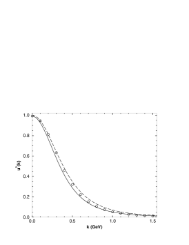
Figure 2: Illustrating that Pauli-Villars regularisation with finite mass-scales is a practical tool. Open circles - $u^{2}(\vec{k})$ calculated directly from Eq. (LABEL:ukdef) using $m_{\pi}=0.14\,$GeV, $M=0.94\,$GeV, $g_{A}=1$ and $\lambda_{1}\to\lambda_{2}=\lambda=0.6\,$GeV; solid line - least-squares fit to $\vec{k}^{2}u^{2}(\vec{k}^{2})$, which yields: $u(\vec{k}^{2})=\mbox{$0.99/(1+\vec{k}^{2}/\bar{\lambda}^{2})^{2}$}$, $\bar{\lambda}=0.54\,$GeV; dashed line - limiting form from Eq. (87).

To provide a quantitative connection with other analyses we employ

$$u(\vec{k})=3\,\frac{j_{1}(|\vec{k}|R)}{|\vec{k}|R}\,;$$ (88)

in Eq. (LABEL:deltaMppCBM); i.e., the CBM form for $u(k)$, where $R$ is the bag radius and $j_{1}(x)$ is a spherical Bessel function. The results are given in Table 2 and may be summarised as (in GeV)

$$-\delta^{A}_{\rm CBM}M_{+}^{+}=(0.065\pm 0.022)\,g_{A}^{2}\,,$$ (89)

where $g_{A}$ is the nucleon’s axial vector coupling constant. (NB. The result in Eq. (89) is also that obtained using a monopole form factor with the very soft scale $\lambda_{\rm CBM}=0.38\pm 0.04\,$GeV.) We stress that in Eqs. (54) and (82) we used the coupling $g=M/f_{\pi}$, Eq. (61), which corresponds to $g_{A}=1$, whereas using the experimental value, $g_{A}=1.26$, Eq. (89) gives

$$\delta^{A}_{\rm CBM}M_{+}^{+}=-0.104\pm 0.035\,{\rm GeV}\,.$$ (90)

The larger shift described in Ref. tonyANU ; tonyCBM is obtained from Eq. (LABEL:deltaMppCBM) by using a smaller bag radius ($\sim 0.75\,$fm), which is needed to describe $\pi N$ scattering. The value of $R$ employed herein is appropriate to the calculation of nucleon electromagnetic form factors tonyR . A priori it is not clear which should be used for the calculation of hadron masses but recent lattice studies Young:2001nc favour a harder value.

Table 2: $\delta^{A}M_{+}^{+}$ calculated using Eq. (88) in Eq. (LABEL:deltaMppCBM); i.e., a CBM estimate. The optimal bag radius for a description of the neutron’s electric form factor is $R=0.95\,{\rm fm}=1/(0.21\,{\rm GeV})$ tonyR .

$R$ (fm)	$0.85$	$0.95$	$1.05$
$-\delta^{A}M_{+}^{+}$  (GeV)	$0.091$	$0.065$	$0.048$

Returning to Eq. (LABEL:AVDSE), the mass-shift contribution from the negative-energy nucleon; i.e., the Z-diagram, is

$$\delta^{A}M_{+}^{-}=\frac{3g^{2}}{16M^{2}}\int\frac{d^{3}k}{(2\pi)^{3}}\frac{1}{\omega_{N}}$$ (91)

$$\times\sum_{i=0,1,2}c_{i}\,\frac{\lambda_{i}^{2}(\omega_{N}+M)+2\vec{k}^{2}(\omega_{\lambda_{i}}+\omega_{N})}{\omega_{\lambda_{i}}[\omega_{\lambda_{i}}+\omega_{N}+M]}.$$

In this case we have $\delta^{A}M_{+}^{+}<0$ and $\delta^{A}M_{+}^{-}>0$ but the sum

$$\delta^{A}M_{+} = \delta^{A}M_{+}^{+}+\delta^{A}M_{+}^{-}$$ (93)

$$= -\,\frac{3g^{2}}{8M^{2}}\int\frac{d^{3}k}{(2\pi)^{3}}\frac{M}{\omega_{N}}$$

$$\times\sum_{i=0,1,2}c_{i}\,\frac{2\vec{k}^{2}\,(\omega_{\lambda_{i}}+\omega_{N})-\lambda_{i}^{2}\,\omega_{\lambda_{i}}}{\omega_{\lambda_{i}}\,(\omega_{N}+\omega_{\lambda_{i}})^{2}-M^{2}}$$

is self-evidently negative; i.e., with a pseudovector coupling the Z-diagram is much suppressed.

Considering the heavy-nucleon limit again one obtains

$$\delta^{A}M_{+}^{+}=-\,\frac{3}{32\pi}\frac{g^{2}}{M^{2}}m_{\pi}^{3}+f^{+}_{(1^{A})}(\lambda_{1},\lambda_{2})\,m_{\pi}^{2}+f^{+}_{(0^{A})}(\lambda_{1},\lambda_{2})\,;$$ (94)

i.e., the same contribution, nonanalytic in the current-quark mass, as in Eq. (76), but with different regularisation-dependent terms. In this case, however, because the Z-diagrams are suppressed by the pseudovector coupling, the leading-order contribution to $\delta^{A}M_{+}^{-}$ is O$(1/M)^{3}$. This is clear from Eq. (91), and makes immediately unambiguous the origin and nature of the leading-order nonanalytic contribution to the nucleon’s mass.

Again interpreting the Pauli-Villars regularisation as introducing a monopole form factor at each $\pi NN$ vertex, we can estimate the magnitude of the $\pi$-loop’s contribution to the nucleon’s mass. Our results are depicted in Fig. 1. It is evident that $\delta^{A}M_{+}^{+}\neq\delta_{F}M_{+}^{+}$, which illustrates the difference between the regularisation-dependent terms in Eqs. (76) and (94). In addition, although it may not be immediately obvious,

$$\delta^{A}M_{+}\equiv\delta M_{+}\,,$$ (95)

which is why there is only one solid curve in the figure. This result provides a quantitative verification of the on-shell equivalence of the pseudoscalar and pseudovector interactions, in perturbation theory, as long as the pseudoscalar interaction is treated in a manner consistent with chiral symmetry sakurai . It also emphasises that, at least for estimating the mass shift, it is advantageous to employ the pseudovector interaction. We note, however, that in fully embracing a Lagrangian density that expresses a nonlinear realisation of chiral symmetry one loses a direct correspondence with extant, ordered truncations of the DSEs, and hence also loses this correspondence between the Lagrangian’s degrees of freedom and hadrons as composites of dressed-quarks.

III.3 Model DSE

We now build on the above analysis and seek a nonperturbative estimate of the $\pi$-loop’s contribution to the nucleon’s mass. Returning to the Euclidean metric described in Appendix A, which is advantageous for numerical studies, the DSE for the nucleon’s self energy using a pseudovector coupling is

$$\Sigma(P) = 3\int\!\frac{d^{4}k}{(2\pi)^{4}}\,g_{PV}^{2}(P,k)\,\Delta_{\pi}((P-k)^{2})\,$$ (96)

$$\times\,\gamma\cdot(P-k)\gamma_{5}\,G(k)\,\gamma\cdot(P-k)\gamma_{5}\,,$$

with the following equivalent representations for the nucleon propagator:

$$G(k) = 1/[i\gamma\cdot k+M+\Sigma(P)]\,,$$ (97)

$$= 1/[i\gamma\cdot k\,{\cal A}(k^{2})+M+{\cal B}(k^{2})]\,,$$ (98)

$$= -i\gamma\cdot k\,\sigma_{\cal V}(k^{2})+\sigma_{\cal S}(k^{2})\,,$$ (99)

where $M$ is the nucleon’s bare mass, which is obtained, e.g., by solving the Faddeev equation. In Eq. (96), $\Delta_{\pi}(k^{2})=1/[k^{2}+m_{\pi}^{2}]$ is the pion propagator, and $g_{PV}(P,k)$ is a form factor that we will use to describe the composite nature of both the pion and the nucleon. The self-consistent solution of Eq. (96) yields ${\cal A}(k^{2})$ and ${\cal B}(k^{2})$, and thereby the nonperturbative mass shift. (For clarity we omit a discussion of renormalisation but remark on its effects following Eq. (124).)

We now turn to the model specified by

$$g_{PV}(P,k)=\frac{g}{2M}\,\exp(-(P-k)^{2}/\Lambda^{2})\,.$$ (100)

The exponential form facilitates an algebraic evaluation of many necessary integrals and, as has been observed elsewhere HLold , is phenomenologically equivalent to a monopole form factor: $1/(1+(P-k)^{2}/\lambda^{2})$, if the mass-scales are related via $\Lambda\approx\sqrt{2}\,\lambda$. Thus one can anticipate a quantitative correspondence between the $\lambda=0.6\,$GeV monopole results of the previous subsections and those obtained in this with $\Lambda\approx 0.9\,$GeV.

Before proceeding with a nonperturbative solution of the nucleon’s DSE we evaluate the one-loop self-energy so as to provide a direct Euclidean space comparison with Secs. III.1, III.2. Using Eq. (100) we can evaluate the $k_{4}$ integral to obtain

$${\cal A}(t^{2})-1$$ (101)

$$= -\frac{3}{32\pi^{2}}\frac{g^{2}}{M^{2}}\int_{0}^{\infty}d\kappa\,\kappa^{2}\,\frac{a(t,\kappa)\,{\rm e}^{-2\kappa^{2}/\Lambda^{2}}}{\omega_{\pi}(\kappa)\,\omega_{N}(\kappa)},$$

$${\cal B}(t^{2}) = -\frac{3}{32\pi^{2}}\frac{g^{2}}{M^{2}}\int_{0}^{\infty}d\kappa\,\kappa^{2}\,\frac{b(t,\kappa)\,{\rm e}^{-2\kappa^{2}/\Lambda^{2}}}{\omega_{\pi}(\kappa)\,\omega_{N}(\kappa)},$$ (102)

where $a(t,\kappa)$, $b(t,\kappa)$ are given in Eqs. (143)-(145). ${\cal A}$ and ${\cal B}$ are plotted in Figs. 3, 4.

Figure 3: Vector piece of the inverse dressed-nucleon propagator. Dotted line: ${\cal A}(t)$ from Eq. (101), ${\cal A}(t=4)=1.001$; solid line: numerical result for the one-loop-dressed function in the spacelike region, obtained from Eqs. (105) - (LABEL:BEDSE), which overlies the dotted line in this region; dashed line: ${\cal A}(t)$ obtained in the self-consistent solution of Eqs. (LABEL:AEDSE), (LABEL:BEDSE); dot-dashed line: ${\cal A}(t)$ (${\cal A}(t=4)=1.002$) obtained in the self-consistent solution of Eqs. (LABEL:AEDSEapp), (LABEL:BEDSEapp) with Eqs. (117), (118) added in the continuation to the timelike region. (All curves obtained with $M=0.94\,$GeV, $m_{\pi}=0.14\,$GeV, $g_{A}=1$, $\Lambda=0.9\,$GeV.)

Figure 4: Scalar piece of the inverse dressed-nucleon propagator. Dotted line: ${\cal B}(t)$ from Eq. (102), $M+{\cal B}(t=4)=0.937\,$GeV; solid line: numerical result for the one-loop-dressed function in the spacelike region, obtained from Eqs. (105) - (LABEL:BEDSE), which overlies the dotted line in this region; dashed line: ${\cal B}(t)$ obtained in the self-consistent solution of Eqs. (LABEL:AEDSE), (LABEL:BEDSE); dot-dashed line: ${\cal B}(t)$ obtained in the self-consistent solution of Eqs. (LABEL:AEDSEapp), (LABEL:BEDSEapp) with Eqs. (117), (118) added in the continuation to the timelike region. (All curves obtained with $M=0.94\,$GeV, $m_{\pi}=0.14\,$GeV, $g_{A}=1$, $\Lambda=0.9\,$GeV.)

The one-loop-corrected nucleon mass: $M_{D^{1}}$, is the solution of

$$M_{D^{1}}^{2}{\cal A}^{2}(-M_{D^{1}}^{2})=[M+{\cal B}(-(M_{D^{1}}^{2})]^{2}\,,$$ (103)

and it is straightforward to show that $M_{D^{1}}-M\equiv\delta M_{+}$, where $\delta M_{+}$ is defined in Eq. (70). The calculated $\Lambda$-dependence of $\delta M_{+}$ is depicted in Fig. 5, and a comparison with Fig. 1 reveals the equivalence between the Minkowski and Euclidean space formulations.

Figure 5: Dashed line: nucleon’s one-loop mass-shift, calculated from ${\cal A}$, ${\cal B}$ in Eqs. (101), (102) - $\delta M_{+}(\Lambda=0.9\,{\rm GeV}\,\approx\sqrt{2}\lambda)=-0.13\,$GeV; dot-dashed line: one-loop mass shift obtained using the approximate kernels in Eqs. (LABEL:KAapprox), (114); solid line: mass shift obtained via the self-consistent solution of the nucleon’s DSE using these approximate kernels - $\delta M_{+}(\Lambda=0.9\,{\rm GeV})=-0.14\,$GeV. The dotted line is $\delta^{A}M_{+}^{+}$; i.e., Eq. (84) calculated in our Euclidean model. (All curves obtained with $M=0.94\,$GeV, $m_{\pi}=0.14\,$GeV, $g_{A}=1$.)

The new feature in a nonperturbative study is that the position of the pole in the nucleon’s propagator is not known a priori: locating it is the goal, and this precludes an algebraic evaluation of the $k_{4}$-integral. The position of the pole will depend on the strength of the interaction and the nature of the form factor. In this case one must proceed by first evaluating the angular integrals in Eq. (96), which are independent of $G(k)$, noting that for a given function of $(P-k)^{2}$:

$$\int d\Omega_{k}\,f((P-k)^{2})=\frac{2}{\pi}\int_{-1}^{1}\!dz\sqrt{1-z^{2}}\,f(P^{2}+k^{2}-2Pkz)\,.$$ (104)

This yields the kernels of the coupled, nonlinear integral equations for ${\cal A}$, ${\cal B}$:

$${\cal K}_{\cal A}(P^{2},k^{2}) = \frac{1}{2}\int\!d\Omega_{k}\,g_{PV}^{2}((P-k)^{2})\bigg{[}-(P^{2}+k^{2})$$ (105)

$$\,+\,\frac{(P^{2}-k^{2})^{2}+m_{\pi}^{2}(P^{2}+k^{2})}{(P-k)^{2}+m_{\pi}^{2}}\bigg{]}\,,$$

$${\cal K}_{\cal B}(P^{2},k^{2}) = \int\!d\Omega_{k}\,g_{PV}^{2}((P-k)^{2})$$ (106)

$$\times\bigg{[}1-\frac{2m_{\pi}^{2}}{(P-k)^{2}+m_{\pi}^{2}}\bigg{]}\,,$$

so that for spacelike $P^{2}$ these integral equations can be written ($x=P^{2}$, $y=k^{2}$)

$$x[{\cal A}(x)-1] = -\,\frac{3}{16\pi^{2}}\int_{0}^{\infty}\!\!dy\,y\,{\cal K}_{\cal A}(x,y)\,\sigma_{\cal V}(y),$$

$${\cal B}(x) = -\,\frac{3}{16\pi^{2}}\int_{0}^{\infty}\!\!dy\,y\,{\cal K}_{\cal B}(x,y)\,\sigma_{\cal S}(y),$$

and solved numerically by iteration.

To illustrate the accuracy attainable with this procedure we: evaluated the integrals in Eqs. (105), (106) numerically for spacelike $P^{2}$; inserted ${\cal A}(k^{2})\equiv 1$ and ${\cal B}(k^{2})=M$ on the r.h.s. of Eqs. (LABEL:AEDSE) and (LABEL:BEDSE); and calculated the integral over $y$ numerically. This yields the estimate of the one-loop-corrected nucleon propagator in the spacelike region depicted in Figs. 3, 4. The agreement with the algebraic result is exact.

The self-consistent solution of Eqs. (LABEL:AEDSE), (LABEL:BEDSE) in the spacelike region is easily obtained by iteration: the one-loop corrected functions are inserted on the r.h.s. to obtain the second iterate, which is then inserted on the r.h.s. to obtain the third iterate, etc., with the procedure repeated until the input and output agree within a specified tolerance. That happens very quickly, with the fourth iterate from free nucleon seed functions (${\cal A}=1$, ${\cal B}=M$) agreeing with the third iterate to better than $10^{-4}\,$%. Hence “three pions in the air” are sufficient to fully dress the nucleon. The functions obtained in this self-consistent solution are also plotted in Figs. 3, 4: only ${\cal A}(t^{2})$ is noticeably modified cf. the one-loop result.

To locate the mass pole in the nonperturbatively dressed nucleon propagator, Eqs. (LABEL:AEDSE), (LABEL:BEDSE) must also be solved for timelike $P^{2}$. That requires an analytic continuation of the kernels in Eqs. (105), (106). The primary nonanalytic feature in their integrands is the pion pole and in continuing to timelike $P^{2}$ it is necessary to properly incorporate its effect. That is difficult when the kernels are only known numerically and an expeditious alternative is to develop an algebraic approximation, which is the approach we adopt.

It is apparent that both kernels can be considered as a sum of two terms. The first is proportional to the angular average of $g_{PV}^{2}((P-k)^{2})$, and using Eq. (100) that integral can be evaluated exactly:

$$\bar{g}_{PV}^{2}(P^{2},k^{2}) := \int d\Omega_{k}\,g_{PV}^{2}((P-k)^{2})$$

$$= \frac{g^{2}}{4M^{2}}\,{\rm e}^{-2(P^{2}+k^{2})/\Lambda^{2}}\,\frac{\Lambda^{2}}{2Pk}\,{\rm I}_{1}(4Pk/\Lambda^{2})\,,$$

where ${\rm I}_{1}(x)$ is a modified Bessel function and $P=\sqrt{P^{2}}$, $k=\sqrt{k^{2}}$. The second term in both cases is proportional to

$$\omega_{g^{2}}(P^{2},k^{2}) := \int d\Omega_{k}\,\frac{g_{PV}^{2}((P-k)^{2})}{(P-k)^{2}+m_{\pi}^{2}}\,,$$ (110)

which, in general, cannot be expressed as a finite sum of known functions. However, if $g_{PV}$ is regular at $P=k$ and its analytic structure is not a key influence on the solution, then the approximation

$$\omega_{g^{2}}(P^{2},k^{2}) \approx g_{PV}^{2}(|P^{2}-k^{2}|)\int\!d\Omega_{k}\,\frac{1}{(P-k)^{2}+m_{\pi}^{2}}$$ (111)

$$= g_{PV}^{2}(|P^{2}-k^{2}|)\,\frac{1}{a+\sqrt{a^{2}-b^{2}}}$$

$$=: \tilde{g}_{PV}^{2}(P^{2},k^{2})\,\frac{1}{a+\sqrt{a^{2}-b^{2}}}\,,$$ (112)

where $a=P^{2}+k^{2}+m_{\pi}^{2}$, $b=2Pk$, is a reliable tool angleapprox . As these preconditions are obviously satisfied in our application – the dominant physical effect in $\pi N$ physics is the pion pole and that appears at a mass-scale much lower than those present in $g_{PV}$ – we pursue our analysis using the following algebraic approximations:

$$\tilde{\cal K}_{\cal A}(x,y) = -\,\frac{1}{2}\,\bar{g}_{PV}^{2}(x,y)\,(x+y)$$

$$+\,\tilde{g}_{PV}^{2}(x,y)\,\frac{(x-y)^{2}+m_{\pi}^{2}(x+y)}{a+\sqrt{a^{2}-b^{2}}}\,,$$

$$\tilde{\cal K}_{\cal B}(x,y) = \bar{g}_{PV}^{2}(x,y)$$ (114)

$$-\,\tilde{g}_{PV}^{2}(x,y)\,\frac{2m_{\pi}^{2}}{a+\sqrt{a^{2}-b^{2}}}\,.$$

To illustrate their efficacy, in Figs. 3, 4 we plot the self-consistent solutions of

$$x[{\cal A}(x)-1] = -\,\frac{3}{16\pi^{2}}\int_{0}^{\infty}\!\!dy\,y\,\tilde{\cal K}_{\cal A}(x,y)\,\sigma_{\cal V}(y),$$

$${\cal B}(x) = -\,\frac{3}{16\pi^{2}}\int_{0}^{\infty}\!\!dy\,y\,\tilde{\cal K}_{\cal B}(x,y)\,\sigma_{\cal S}(y).$$

The error introduced by the approximation is never more than $1$% and is only that large for ${\cal A}(t^{2}=0)$.

We can now define the model’s analytic continuation to the timelike region. The approximate kernels’ primary nonanalyticity is a square-root branch point whose appearance and location are tied to the simple pole in the pion propagator, and in continuing to $P^{2}<0$ it is necessary to include the discontinuity across the associated cut. That is accomplished fukuda76 by adding the following additional terms to the r.h.s. of Eqs. (LABEL:AEDSEapp), (LABEL:BEDSEapp), respectively:

$$-\frac{3}{16\pi^{2}}\int_{x_{b}}^{0}\!\!dy\,y\,\hat{g}^{2}(x,y)\,\Delta\tilde{\cal K}_{\cal A}(x,y)\,\sigma_{\cal V}(y)\,,$$ (117)

$$-\frac{3}{16\pi^{2}}\int_{x_{b}}^{0}\!\!dy\,y\,\hat{g}^{2}(x,y)\,\Delta\tilde{\cal K}_{\cal B}(x,y)\,\sigma_{\cal S}(y)\,,$$ (118)

where

$$\Delta\tilde{\cal K}_{\cal A}(x,y)=-\,\frac{\Delta{\cal K}_{\cal B}(x,y)}{2\,m_{\pi}^{2}}\,\left[(x-y)^{2}+m_{\pi}^{2}(x+y)\right]\,,$$ (119)

$$\Delta\tilde{\cal K}_{\cal B}(x,y) = m_{\pi}^{2}\,\frac{\sqrt{(x+y+m_{\pi}^{2})^{2}-4xy}}{x\,y}\,,$$ (120)

and $y=x_{b}=-(\sqrt{-x}-m_{\pi})^{2}$ is the location of the branch point. (NB. These terms are present only when $P^{2}+m_{\pi}^{2}<0$.) The self-consistent solutions of Eqs. (LABEL:AEDSEapp)-(118) are depicted in Figs. 3, 4 and unsurprisingly there is little difference between the one-loop results and the self-consistent solution.

In Fig. 5 we compare the exact one-loop mass shift with that obtained numerically using the approximate kernels. The error is never more than $5$% with the approximation always overestimating the magnitude of the shift. (It is noteworthy that a large part of the one-loop mass-shift is due to the vector self energy; e.g., with $\Lambda=0.9\,$GeV, $(\delta M_{+})_{\rm one-loop}$ is $40\,$% smaller if the vector self-energy is neglected.)

The fully dressed nucleon mass, $M_{D}$, is obtained by solving

$$M_{D}^{2}{\cal A}^{2}(-M_{D}^{2})=[M+{\cal B}(-M_{D}^{2})]^{2}$$ (121)

with the nonperturbative mass shift given by $\delta M_{+}=M_{D}-M$. Again, this definition is completely equivalent to Eq. (70) evaluated at $M_{D}$ with the self-consistent solution of the DSE. The $\Lambda$-dependence of the nonperturbative shift is also depicted in Fig. 5 and comparison with the numerical one-loop result shows that the additional pion dressing adds $\lesssim 5\,$% to $|\delta M_{+}|$.

Thus far we have used our Euclidean model to quantitatively reproduce the perturbative results of Secs. III.1, III.2 and thereby make transparent the equivalence of the Euclidean and Minkowski formulations. In addition we have shown that the one-loop mass shift is $\sim 95$% of the total.

However, we have not yet considered an effect of nucleon compositeness. A covariant $\pi NN$ vertex function must depend on three independent variables: $g_{PV}=g_{PV}(P^{2},k^{2},(P-k)^{2})$ mr97 , and hitherto we have neglected its dependence on $P^{2}$, $k^{2}$. (We have already seen that $g_{PV}=g_{PV}((P-k)^{2})$ corresponds to a Pauli-Villars regularisation of the pion propagator alone.) The calculation of form factors that describe interactions between composite objects; e.g., studies of the $\rho$-$\omega$ mass splitting rhopipipeter ; rhopipi and electromagnetic form factors pieterGamma ; revbasti ; weiss ; gstarpig , indicates that the $\pi NN$ vertex should also suppress the pion-nucleon coupling when the nucleons are off-shell. We conduct an initial, exploratory study of this effect by considering the product Ansatz

$$g_{PV}(P^{2},k^{2},P\cdot k)=$$ (122)

$$\frac{g}{2M}\,{\rm e}^{-(P-k)^{2}/\Lambda^{2}}\,{\rm e}^{-(P^{2}+M^{2}+k^{2}+M^{2})/\Lambda_{N}^{2}}\,,$$

which reduces to Eq. (100) when $\Lambda_{N}\to\infty$ and guarantees $g_{PV}(-M^{2},-M^{2},0)=g/(2M)$, as required. Previous applications of such a form factor in the $\pi N$ sector pearcea typically require

$$\Lambda_{N}/\Lambda\sim 1.5\,-2.0\,.$$ (123)

(NB. While $\Lambda_{N}$ is calculable using a covariant model of the nucleon, no such calculations exist and to constrain its value we must currently rely on phenomenology.) The effect on the mass shift of this off-shell suppression is depicted in Fig. 6: it is significant, leading to a reduction of $\gtrsim 50\,$% in $|\delta M_{+}|$. For $\Lambda_{N}\to\infty$; i.e., in the absence of the off-shell suppression, this effect can be mimicked by a reduction in $\Lambda$; e.g., $\Lambda\to\Lambda^{\prime}=0.7\,$GeV yields $\delta M_{+}=-0.07\,$GeV, and we note that $\Lambda^{\prime}/\sqrt{2}=0.5\,$GeV, which is commensurate with $\lambda_{\rm CBM}\approx 0.4\,$GeV, after Eq. (89).

Figure 6: Effect on the mass-shift produced by including nucleon-off-shell suppression in the $\pi NN$ vertex: Eq. (122), for $\Lambda=0.9\,$GeV, $m_{\pi}=0.14\,$GeV. (NB. $\delta M_{+}(\Lambda=0.9\,{\rm GeV},\Lambda_{N}=\infty)=-0.14\,$GeV.)

Combining all the elements of our analysis we arrive at a result for the shift in the nucleon’s mass owing to the $\pi N$-loop (for $g_{A}=1.26$, in GeV):

$$-\delta M_{+}\simeq(0.039-0.063)\,g_{A}^{2}=(0.061-0.099)\,.$$ (124)

In the preceding, for illustrative clarity, we did not account for the effects of finite vertex renormalisation; i.e., we set $Z_{1}=1=Z_{2}$ in Eq. (96). Studies using the CBM indicate that a quantitative description of $\pi N$ vertex renormalisation requires that the $\Delta$ be treated on an equal footing with the nucleon and that this is crucial to obtaining a convergent expansion tonyCBM ; Dodd:pw . Indeed, one finds, as here, that the $\pi$-loop acts to suppress the nucleon’s wave-function renormalisation; i.e., it forces $Z_{2}<1$, but in the CBM this effect is compensated by an almost matching suppression of $Z_{1}$ so that the bare and renormalised $\pi N$ couplings are little different. A self-consistent, covariant treatment of the coupled composite-$N$-$\Delta$ system is more than we are able to describe herein. However, the CBM studies suggest that a reliable estimate of the effect of including the $\Delta$ can be obtained simply by solving an analogue of Eq. (96) with $Z_{1}=Z_{2}$ for a renormalised model.

We have done this and thereby arrive at a robust result: the $\pi N$-loop reduces the nucleon’s mass by $\sim 10\,$-$\,20$% fn:error . Extant calculations; e.g., Refs. tonyANU ; tonyCBM ; harry , show that the contribution from the analogous $\pi\Delta$-loop is of the same sign and no greater in magnitude so that the likely total reduction is $20\,$-$\,40$%. Based on these same calculations we anticipate that the $\Delta$ mass is also reduced by $\pi$ loops but by a smaller amount ($\sim 50\,$-$\,100\,$MeV less).

How does that affect the quark-diquark picture of baryons? To address this issue we again solved the Faddeev equations, this time requiring that the quark-diquark component yield higher masses for the $N$ and $\Delta$: $M_{N}=0.94+0.2=1.14\,$GeV, $M_{\Delta}=1.232+0.1=1.332\,$GeV. The results, presented in the third and fourth rows of Table 1, establish that the effects are not large. In this case omitting the axial-vector diquark yields $M_{N}=1.44\,$GeV, which signals a $10\,$% increase in the importance of the scalar-diquark component of the nucleon. (It is an increase because this component now requires less correction. Note, too, that the scalar diquark’s charge radius, $r_{0^{+}}=0.63\,$fm, is $15\,$% larger.) It also announces a reduction in the role played by axial-vector diquark correlations in the nucleon, since now restoring them only reduces the nucleon’s core mass by $21$%, with $\pi$ self-energy corrections providing the remaining $14$%. It is thus apparent that requiring an exact fit to the $N$ and $\Delta$ masses using only quark and diquark degrees of freedom leads to an overestimate of the role played by axial-vector diquark correlations: it forces the $1^{+}$ diquark to mimic, in part, the effect of pions since they both act to reduce the mass cf. that of a quark$+$scalar-diquark baryon.

IV Epilogue

We showed that an internally consistent description of the $N$ and $\Delta$ masses is easily obtained using a Poincaré covariant Faddeev equation that represents baryons as composites of a confined-quark and -diquark. We term this the “core mass” of the baryons. They are weakly bound in the limited sense that the sum of the masses of their primary constituents is little greater than their core mass.

The on-shell $\pi NN$ and $\pi N\Delta$ couplings are large and hence it is conceivable that $\pi N$ and $\pi\Delta$ self-energy corrections to the nucleon’s mass may be significant. We therefore studied the effects of the $\pi N$-loop on the nucleon’s core mass and found that, in well-constrained models, this loop reduces that mass by $\lesssim 20$%. Including the $\pi\Delta$ self-energy contribution, the total reduction is likely to be between $20$ and $40$%. While this is a material effect it does not undermine the qualitative picture of baryons suggested by the Faddeev equation; namely, that baryons are primarily quark-diquark composites. This is consistent with the fact that a converged nonperturbative calculation of the $\pi$-induced self-energy requires only three “pions in the air,” but to be certain we re-solved the Faddeev equation aiming at nucleon and $\Delta$ masses corrected for the $\pi$ self-energy contribution, and found little change in the character of the solution.

The one notable effect was a material reduction in the nucleon’s axial-vector diquark component. This is easily understood: ignoring $\pi$-loops forces the axial-vector diquarks to mimic their effect. That surrogacy cannot be completely effective and may have led to quantitative errors, and errors of interpretation, in contemporary quark-diquark based calculations of quantities such as the neutron’s charge form factor and the ratio $\mu_{p}G_{E}^{p}/G_{M}^{p}$. Our results should serve as a signal of this possibility and stimulate increased caution and an objective reanalysis.

Our exploration of the role of $\pi$-loops was pedagogical. We made clear that the leading nonanalytic contribution to the nucleon’s mass arises from that part of the loop integral which corresponds to a positive-energy nucleon; i.e., whether the $\pi NN$ coupling is pseudoscalar or pseudovector, the $Z$-diagrams do not affect the leading nonanalytic behaviour. Furthermore, we showed explicitly that the one-loop mass shift calculated with a pseudoscalar coupling is precisely the same as that obtained with a pseudovector coupling, so long as, and only if, no diagrams are overlooked in the pseudoscalar calculation. We illustrated that, using any translationally invariant regularisation procedure which preserves information about the pion’s finite size, the tadpole (Hartree) diagram generated by a pseudoscalar coupling cannot be neglected because it balances the very large contribution from the pseudoscalar $Z$-diagram. This result should not be overlooked in the phenomenological application of model field theories founded on hadronic degrees of freedom.

Appendix A Euclidean Conventions

A.1 Metric and Spinors

In our Euclidean formulation:

$$p\cdot q=\sum_{i=1}^{4}p_{i}q_{i}\,;$$ (125)

$$\{\gamma_{\mu},\gamma_{\nu}\}=2\,\delta_{\mu\nu}\,;\;\gamma_{\mu}^{\dagger}=\gamma_{\mu}\,;\;\sigma_{\mu\nu}=\mbox{\footnotesize$\displaystyle\frac{i}{2}$}[\gamma_{\mu},\gamma_{\nu}]\,;$$ (126)

$${\rm tr}_{[}\gamma_{5}\gamma_{\mu}\gamma_{\nu}\gamma_{\rho}\gamma_{\sigma}]=-4\,\epsilon_{\mu\nu\rho\sigma}\,,\epsilon_{1234}=1\,.$$ (127)

A positive energy spinor satisfies

$$\bar{u}(P,s)\,(i\gamma\cdot P+M)=0=(i\gamma\cdot P+M)\,u(P,s)\,,$$ (128)

where $s=\pm$ is the spin label. It is normalised:

$$\bar{u}(P,s)\,u(P,s)=2M$$ (129)

and may be expressed explicitly:

$$u(P,s)=\sqrt{M-i{\cal E}}\left(\begin{array}[]{l}\chi_{s}\\ \displaystyle\frac{\vec{\sigma}\cdot\vec{P}}{M-i{\cal E}}\chi_{s}\end{array}\right)\,,$$ (130)

with ${\cal E}=i\sqrt{\vec{P}^{2}+M^{2}}$,

$$\chi_{+}=\left(\begin{array}[]{c}1\\ 0\end{array}\right)\,,\;\chi_{-}=\left(\begin{array}[]{c}0\\ 1\end{array}\right)\,.$$ (131)

For the free-particle spinor, $\bar{u}(P,s)=u(P,s)^{\dagger}\gamma_{4}$.

The spinor can be used to construct a positive energy projection operator:

$$\Lambda_{+}(P):=\frac{1}{2M}\,\sum_{s=\pm}\,u(P,s)\,\bar{u}(P,s)=\frac{1}{2M}\left(-i\gamma\cdot P+M\right).$$ (132)

A negative energy spinor satisfies

$$\bar{v}(P,s)\,(i\gamma\cdot P-M)=0=(i\gamma\cdot P-M)\,v(P,s)\,,$$ (133)

and possesses properties and satisfies constraints obtained via obvious analogy with $u(P,s)$.

A charge-conjugated Bethe-Salpeter amplitude is obtained via

$$\bar{\Gamma}(k;P)=C^{\dagger}\,\Gamma(-k;P)^{\rm T}\,C\,,$$ (134)

where “T” denotes a transposing of all matrix indices and $C=\gamma_{2}\gamma_{4}$ is the charge conjugation matrix, $C^{\dagger}=-C$.

In describing the $\Delta$ resonance we employ a Rarita-Schwinger spinor to unambiguously represent a covariant spin-$3/2$ field. The positive energy spinor is defined by the following equations:

$$(i\gamma\cdot P+M)\,u_{\mu}(P;r) = 0\,,$$ (135)

$$\gamma_{\mu}u_{\mu}(P;r) = 0\,,$$ (136)

$$P_{\mu}u_{\mu}(P;r) = 0\,,$$ (137)

where $r=-3/2,-1/2,1/2,3/2$. It is normalised:

$$\bar{u}_{\mu}(P;r^{\prime})\,u_{\mu}(P;r)=2M\,,$$ (138)

and satisfies a completeness relation

$$\frac{1}{2M}\sum_{r=-3/2}^{3/2}u_{\mu}(P;r)\,\bar{u}_{\nu}(P;r)=\Lambda_{+}(P)\,R_{\mu\nu}\,,$$ (139)

where

$$R_{\mu\nu}=\delta_{\mu\nu}I_{\rm D}-\frac{1}{3}\gamma_{\mu}\gamma_{\nu}+\frac{2}{3}\hat{P}_{\mu}\hat{P}_{\nu}I_{\rm D}-i\frac{1}{3}[\hat{P}_{\mu}\gamma_{\nu}-\hat{P}_{\nu}\gamma_{\mu}]\,,$$ (140)

with $\hat{P}^{2}=-1$, which is very useful in simplifying the positive energy $\Delta$’s Faddeev equation.

A.2 Euclidean One-loop Calculations

In Eqs. (101) and (102)

$$a(t,\kappa) = -a_{0}(t,\kappa)+a_{1}(t,\kappa)+a_{2}(t,\kappa)\,,$$ (141)

$$b(t,\kappa) = a_{0}(t,\kappa)+a_{2}(t,\kappa)\,,$$ (142)

where

$$a_{0}(t,\kappa)=$$ (143)

$$\kappa^{2}\bigg{[}{\cal I}_{0}(\omega_{\pi}(\kappa))\,\sum_{s=0}^{1}\frac{\omega_{N}(\kappa)+(-)^{s}\omega_{\pi}(\kappa)}{(\omega_{N}(\kappa)+(-)^{s}\omega_{\pi}(\kappa))^{2}+t^{2}}$$

$$-{\cal I}_{0}(\Omega_{N}(t,\kappa))\,\frac{\omega_{\pi}(\kappa)}{\Omega_{N}^{2}(t,\kappa)-\omega_{\pi}^{2}(\kappa)}$$

$$-{\cal I}_{0}(\bar{\Omega}_{N}(t,\kappa))\,\frac{\omega_{\pi}(\kappa)}{\bar{\Omega}_{N}^{2}(t,\kappa)-\omega_{\pi}^{2}(\kappa)}\bigg{]},$$

$$a_{1}(t,\kappa)=m_{\pi}^{2}\,\omega_{\pi}(\kappa)$$ (144)

$$\times \bigg{[}{\cal I}_{0}(\omega_{\pi}(\kappa))\,\sum_{s=0}^{1}\frac{(-)^{s}}{(\omega_{N}(\kappa)+(-)^{s}\omega_{\pi}(\kappa))^{2}+t^{2}}$$

$$+\frac{i}{t}\,{\cal I}_{0}(\Omega_{N}(t,\kappa))\,\frac{\Omega_{N}(t,\kappa)}{\Omega_{N}^{2}(t,\kappa)-\omega_{\pi}^{2}(\kappa)}$$

$$-\frac{i}{t}\,{\cal I}_{0}(\bar{\Omega}_{N}(t,\kappa))\,\frac{\bar{\Omega}_{N}(t,\kappa)}{\bar{\Omega}_{N}^{2}(t,\kappa)-\omega_{\pi}^{2}(\kappa)}\bigg{]},$$

$$- \frac{i}{t}\,\omega_{\pi}(\kappa)\,\bigg{[}\Omega_{N}(t,\kappa)\,{\cal I}_{0}(\Omega_{N}(t,\kappa))$$

$$-\bar{\Omega}_{N}(t,\kappa)\,{\cal I}_{0}(\bar{\Omega}_{N}(t,\kappa))\bigg{]}$$

$$a_{2}(t,\kappa)=$$ (145)

$$\bigg{[}{\cal I}_{2}(\omega_{\pi}(\kappa))\,\sum_{s=0}^{1}\frac{\omega_{N}(\kappa)+(-)^{s}\omega_{\pi}(\kappa)}{(\omega_{N}(\kappa)+(-)^{s}\omega_{\pi}(\kappa))^{2}+t^{2}}$$

$$-{\cal I}_{2}(\Omega_{N}(t,\kappa))\,\frac{\omega_{\pi}(\kappa)}{\Omega_{N}^{2}(t,\kappa)-\omega_{\pi}^{2}(\kappa)}$$

$$-{\cal I}_{2}(\bar{\Omega}_{N}(t,\kappa))\,\frac{\omega_{\pi}(\kappa)}{\bar{\Omega}_{N}^{2}(t,\kappa)-\omega_{\pi}^{2}(\kappa)}\bigg{]},$$

where $\Omega_{N}(t,\kappa)=\omega_{N}(\kappa)+it$, $\bar{\Omega}_{N}(t,\kappa)=\omega_{N}(\kappa)-it$, and

$${\cal I}_{0}(x) := 2\int_{0}^{\infty}du\,{\rm e}^{-2u^{2}/\Lambda^{2}}\frac{1}{x-iu}$$ (146)

$$= {\rm e}^{\,2x^{2}/\Lambda^{2}}\,{\rm erfc}(x\sqrt{2}/\Lambda)\,,$$

$${\cal I}_{2}(x) := 2\int_{0}^{\infty}du\,{\rm e}^{-2u^{2}/\Lambda^{2}}\frac{u^{2}}{x-iu}$$ (147)

$$= x\bigg{(}\frac{\Lambda}{\sqrt{2\pi}}-x\,{\cal I}_{0}(x)\bigg{)}\,,$$

where ${\rm erfc}(x)$ is the complementary error function and both these functions are odd under $x\to-x$.

References

• (1) A.W. Thomas and W. Weise, “The Structure Of The Nucleon” (Wiley-VCH, Berlin, 2001).
• (2) L. Wilets, “Nontopological Solitons” (World Scientific, Singapore, 1989).
• (3) M.C. Birse, Prog. Part. Nucl. Phys.  25, 1 (1990).
• (4) R. Alkofer and H. Reinhardt, “Chiral quark dynamics” (Springer Verlag, Berlin, 1995); J. Schechter and H. Weigel, “The Skyrme Model for Baryons,” in Quantum Field Theory: a 20th Century Profile, edited by A.N. Mitra (Hindustan Publ., New Delhi, 2000) pp. 337-369
• (5) A.W. Thomas, S. Theberge and G.A. Miller, Phys. Rev. D 24, 216 (1981); A.W. Thomas, Adv. Nucl. Phys.  13, 1 (1984); G.A. Miller, Int. Rev. Nucl. Phys.  1, 189 (1985).
• (6) A.W. Thomas and S.V. Wright, “Classical Quark Models: An Introduction,” in Frontiers in Nuclear Physics: From Quark-Gluon Plasma to Supernova, edited by S. Kuyucak (World Scientific, Singapore, 1999) pp. 171-211.
• (7) S. Capstick and W. Roberts, Prog. Part. Nucl. Phys. 45, S241 (2000).
• (8) G.A. Miller and A.W. Thomas, Phys. Rev. C 56, 2329 (1997).
• (9) F. Coester, Prog. Part. Nucl. Phys. 29, 1 (1992); F. Coester and W.N. Polyzou, “Relativistic Quantum Dynamics of Many-Body Systems,” nucl-th/0102050.
• (10) R. T. Cahill, J. Praschifka and C. Burden, Austral. J. Phys.  42, 161 (1989).
• (11) R.T. Cahill and C.D. Roberts, Phys. Rev. D 32, 2419 (1985).
• (12) P.C. Tandy, Prog. Part. Nucl. Phys. 39, 117 (1997).
• (13) R.T. Cahill and S.M. Gunner, Fizika B 7, 171 (1998).
• (14) R.T. Cahill, C.D. Roberts and J. Praschifka, Austral. J. Phys. 42, 129 (1989).
• (15) C.J. Burden, R.T. Cahill and J. Praschifka, Austral. J. Phys. 42, 147 (1989).
• (16) H. Asami, N. Ishii, W. Bentz and K. Yazaki, Phys. Rev. C 51, 3388 (1995); H. Mineo, W. Bentz and K. Yazaki, ibid. 60, 065201 (1999).
• (17) M. Oettel, G. Hellstern, R. Alkofer and H. Reinhardt, Phys. Rev.  C 58, 2459 (1998).
• (18) M. Oettel, R. Alkofer and L. von Smekal, Eur. Phys. J. A 8, 553 (2000).
• (19) J.C.R Bloch, C.D. Roberts, S.M. Schmidt, A. Bender and M.R. Frank, Phys. Rev. C 60, 062201 (1999).
• (20) J.C.R. Bloch, C.D. Roberts and S.M. Schmidt, Phys. Rev. C 61, 065207 (2000).
• (21) M.B. Hecht, C.D. Roberts and S.M. Schmidt, “Contemporary applications of Dyson-Schwinger equations,” nucl-th/0010024.
• (22) M.B. Hecht, C.D. Roberts and S.M. Schmidt, Phys. Rev. C 64, 025204 (2001).
• (23) B.C. Pearce and I.R. Afnan, Phys. Rev. C 34, 991 (1986).
• (24) N. Ishii, Phys. Lett. B 431, 1 (1998).
• (25) E.J. Hackett-Jones, D.B. Leinweber and A.W. Thomas, Phys. Lett. B 489, 143 (2000); ibid. 494, 89 (2000); D.B. Leinweber, A.W. Thomas and R.D. Young, Phys. Rev. Lett.  86, 5011 (2001).
• (26) D.B. Leinweber, A.W. Thomas, K. Tsushima and S.V. Wright, Phys. Rev. D 61, 074502 (2000).
• (27) R.D. Young, D.B. Leinweber, A.W. Thomas and S.V. Wright, “Systematic correction of the chiral properties of quenched QCD,” hep-lat/0111041.
• (28) C.D. Roberts and A.G. Williams, Prog. Part. Nucl. Phys. 33, 477 (1994).
• (29) P. Maris and C.D. Roberts, Phys. Rev. C 56, 3369 (1997).
• (30) P. Maris and P.C. Tandy, Phys. Rev. C 60, 055214 (1999);
• (31) P. Maris and P.C. Tandy, Phys. Rev. C 61, 045202 (2000); ibid. 62, 055204 (2000); C.-R Ji and P. Maris, Phys. Rev. D 64, 014032 (2001).
• (32) I.R. Afnan and A.W. Thomas, “Fundamentals of three body scattering theory,” in Topics in Current Physics, Vol. 4 (Springer-Verlag, Berlin, 1977) pp. 1-47.
• (33) C.J. Burden, L. Qian, C.D. Roberts, P.C. Tandy and M.J. Thomson, Phys. Rev. C 55, 2649 (1997).
• (34) R.T. Cahill and S.M. Gunner, Phys. Lett. B 359, 281 (1995).
• (35) P. Maris, “Dyson-Schwinger equations and $\pi\pi$ scattering,” presented at the Tübingen Workshop on Quarks and Hadrons in Continuum Strong QCD, Universität Tübingen, Germany, 3-6/Sept./2001, unpublished: the model of Ref. pieterrho yields $m_{qq_{0^{+}}}=0.82\,$GeV, $m_{qq_{1^{+}}}=1.03\,$GeV.
• (36) M. Hess, F. Karsch, E. Laermann and I. Wetzorke, Phys. Rev. D 58, 111502 (1998).
• (37) F.E. Close and A.W. Thomas, Phys. Lett. B 212, 227 (1988); A.W. Schreiber, A.I. Signal and A.W. Thomas, Phys. Rev. D 44, 2653 (1991); M. Alberg, E.M. Henley, X.D. Ji and A.W. Thomas, Phys. Lett. B 389, 367 (1996).
• (38) Herein we almost exclusively employ a Euclidean metric, which is described in Appendix A. A Minkowski metric is used only in sections III.1, III.2.
• (39) C.D. Roberts and S.M. Schmidt, Prog. Part. Nucl. Phys. 45, S1 (2000).
• (40) R. Alkofer and L. von Smekal, Phys. Rept. 353, 281 (2001).
• (41) J.I. Skullerud and A.G. Williams, Phys. Rev. D 63, 054508 (2001).
• (42) P. Maris, “Continuum QCD and light mesons,” nucl-th/0009064.
• (43) P.C. Tandy, “Soft QCD modeling of meson electromagnetic form factors,” in Lepton Scattering, Hadrons and QCD, edited by W. Melnitchouk, A.W. Schreiber, A.W. Thomas and P.C. Tandy (World Scientific, Singapore, 2001) pp. 192-200.
• (44) C.J. Burden, C.D. Roberts and M.J. Thomson, Phys. Lett. B 371, 163 (1996).
• (45) M.A. Ivanov, Yu.L. Kalinovsky and C.D. Roberts, Phys. Rev. D 60, 034018 (1999).
• (46) P. Maris, C.D. Roberts and P.C. Tandy, Phys. Lett. B 420, 267 (1998).
• (47) H.J. Munczek, Phys. Lett. B 175, 215 (1986); C.J. Burden, C.D. Roberts and A.G. Williams, Phys. Lett. B 285, 347 (1992).
• (48) This is a sufficient condition for confinement because of the associated violation of reflection positivity, as discussed, e.g., in Sec. 6.2 of Ref. cdragw , Sec. 2.2 of Ref. revbasti and Sec. 2.4 of Ref. revreinhard .
• (49) S. Ahlig, R. Alkofer, C. Fischer, M. Oettel, H. Reinhardt and H. Weigel, Phys. Rev. D 64, 014004 (2001).
• (50) M.B. Hecht, C.D. Roberts and S.M. Schmidt, “The character of Goldstone bosons,” in Lepton Scattering, Hadrons and QCD, edited by W. Melnitchouk, A.W. Schreiber, A.W. Thomas and P.C. Tandy (World Scientific, Singapore, 2001) pp. 219-227.
• (51) A. Bender, C.D. Roberts and L. von Smekal, Phys. Lett. B 380, 7 (1996).
• (52) R.T. Cahill, C.D. Roberts and J. Praschifka, Phys. Rev. D 36, 2804 (1987).
• (53) J.C.R Bloch, Yu.L. Kalinovsky, C.D. Roberts and S.M. Schmidt, Phys. Rev. D 60, 111502 (1999).
• (54) C.D. Roberts, R.T. Cahill, M.E. Sevior and N. Iannella, Phys. Rev. D 49, 125 (1994).
• (55) S.L. Adler, Phys. Rev.  137, B1022 (1965).
• (56) J.J. Sakurai, “Remarks on Low-Energy $\pi N$ Scattering,” in Pion-Nucleon Scattering, edited by G.L. Shaw and D.Y. Wong (Wiley, New York, 1969) pp. 209-213.
• (57) See also Fig. 2 and the associated discussion.
• (58) R.T. Cahill, Nucl. Phys. A 543, 63C (1992).
• (59) K.L. Mitchell and P.C. Tandy, Phys. Rev. C 55, 1477 (1997).
• (60) A.W. Thomas and K. Holinde, Phys. Rev. Lett.  63, 2025 (1989).
• (61) The sign before the integral in Eq. (65) of Ref. gunnergcm is incorrect.
• (62) S. Weinberg, Phys. Rev.  166, 1568 (1968).
• (63) A.W. Thomas, J. Phys. G 7, L283 (1981).
• (64) T.-S.H. Lee, private communication.
• (65) D.H. Lu, S.N. Yang and A.W. Thomas, Nucl. Phys. A 684, 296 (2001).
• (66) M.A. Ivanov, Yu.L. Kalinovsky, P. Maris and C.D. Roberts, Phys. Rev. C 57, 1991 (1998).
• (67) C.D. Roberts and B.H.J. McKellar, Phys. Rev. D 41, 672 (1990); H.J. Munczek and D.W. McKay, Phys. Rev. D 42, 3548 (1990).
• (68) R. Fukuda and T. Kugo, Nucl. Phys. B 117, 250 (1976).
• (69) L.C.L. Hollenberg, C.D. Roberts and B.H.J. McKellar, Phys. Rev. C 46, 2057 (1992); M.A. Pichowsky, S. Walawalkar and S. Capstick, Phys. Rev. D 60, 054030 (1999).
• (70) C. Weiss, Phys. Lett.  B 333, 7 (1994).
• (71) M.R. Frank, K.L. Mitchell, C.D. Roberts and P. C. Tandy, Phys. Lett. B 359, 17 (1995).
• (72) B.C. Pearce and B.K. Jennings, Nucl. Phys. A 528, 655 (1991).
• (73) L.R. Dodd, A.W. Thomas and R.F. Alvarez-Estrada, Phys. Rev. D 24, 1961 (1981).
• (74) The estimate of $\delta M_{+}$ in Ref. cdrqciv is incorrect because that calculation overlooked the tadpole (Hartree) term and the contribution at timelike momenta associated with the branch cut in the kernel.