Oscillations in finite Fermi systems

Abstract

A semiclassical linear response theory based on the Vlasov equation is reviewed. The approach discussed here differs from the classical one of Vlasov and Landau for the fact that the finite size of the system is explicitly taken into account. The non-trivial problem of deciding which boundary conditions are more appropriate for the fluctuations of the phase-space density has been circumvented by studying solutions corresponding to different boundary conditions (fixed and moving surface). The fixed-surface theory has been applied to systems having both spherical and spheroidal equilibrium shapes. The moving-surface theory is related to the liquid-drop model of the nucleus and from it one can obtain a kinetic-theory description of surface and compression modes in nuclei. Quantum corrections to the semiclassical theory are also briefly discussed.

1 INTRODUCTION

In this paper we review the work of our groups on the application of the Vlasov kinetic equation to small-amplitude density vibrations in finite Fermi systems. The phenomenology that is described by this approach includes giant resonances in nuclei, surface plasmons in atomic clusters and possible collective excitations of the electrons in heavy atoms (which however turned out not to be really collective). In the approach of Jeans [1], Vlasov [2, 3] and Landau [4, 5] the theory has been developed for infinite homogeneous systems, later Kirzhnitz et al. [6] extended it to non-uniform systems.

The quantity that is studied in this approach is the phase-space density (or single-particle distribution) $f({\bf r},{\bf p},t)$. This quantity, when multiplied by the phase space volume $d{\bf r}d{\bf p}$ gives the number of particles contained in that volume and has several useful properties since its knowledge allows us to obtain information about macroscopic properties of the system like, for example, the ordinary density

$$\varrho({\bf r},t)=\int d{\bf p}f({\bf r},{\bf p},t)\,,$$ (1)

or the pressure tensor

$$\Pi_{jk}({\bf r},t)=\int d{\bf p}p_{j}v_{k}f({\bf r},{\bf p},t)\,.$$ (2)

We limit our interest to small oscillations of $f({\bf r},{\bf p},t)$ about its equilibrium value $f_{0}({\bf r},{\bf p})$, which is supposed to describe the stationary state of the many-body system. If the system is subject to a weak external driving potential $V_{ext}({\bf r},t)=\beta(t)Q({\bf r})$, then $f_{0}$ is changed by the small amount $\delta f({\bf r},{\bf p},t)$, consequently the local equilibrium density also changes by

$$\delta\varrho({\bf r},t)=\int d{\bf p}\delta f({\bf r},{\bf p},t)\,,$$ (3)

and the equilibrium mean field $V_{0}({\bf r})$ by

$$\delta V({\bf r},t)=\int d{\bf r}^{\prime}v({\bf r},{\bf r}^{\prime})\delta\varrho({\bf r}^{\prime},t)\,.$$ (4)

The quantity $v({\bf r},{\bf r}^{\prime})$ is the effective interaction between two constituents of the many-body system. We shall consider only quantities at first order in $\delta f$, moreover the equilibrium distribution will be assumed to depend only on the energy of the particles: $f_{0}({\bf r},{\bf p})=F(h_{0}({\bf r},{\bf p}))$, where

$$h_{0}({\bf r},{\bf p})=\frac{p^{2}}{2m}+V_{0}({\bf r})$$ (5)

is the equilibrium hamiltonian.

In a fully self-consistent approach the equilibrium mean field should be given by

$$V_{0}({\bf r})=\int d{\bf r}^{\prime}v({\bf r},{\bf r}^{\prime})\int d{\bf p}f_{0}({\bf r}^{\prime},{\bf p})\,,$$ (6)

however we shall use phenomenological approximations to it. There are two kinds of self-consistency requirements: the static self-consistency expressed by Eq. (6), and the analogous dynamic self-consistency condition (4). We shall treat the static self-consistency condition more loosely, but will respect the dynamic condition (4) because it is essential in the description of collective modes.

2 HISTORICAL
REMARKS

The following differential equation for $f({\bf r},{\bf p},t)$ was considered by A.A. Vlasov in a study of plasma oscillations [2, 3]:

$$\frac{\partial f}{\partial t}+\frac{{\bf p}}{m}\frac{\partial f}{\partial{\bf r}}-(\frac{\partial V}{\partial{\bf r}})\cdot{{\partial f}\over{\partial{\bf p}}}=0\,,$$ (7)

together with the Poisson equation

$$\nabla^{2}V=-4\pi e^{2}\varrho\,.$$ (8)

Because of Eq.(1), equations (7) and (8) form a set of coupled equations that can be solved self-consistently. Thus the kinetic equation (7), supplemented by (8), can be considered as a dynamical generalization of the static Thomas-Fermi method.

Althogh Eq.(7) is a simplified version of an equation already derived by Boltzmann and the idea of self-consistency in connection with it had already been used by Jeans (see [7] for a discussion of hystorical priorities), we follow the use common both in plasma and in nuclear physics, and refer to Eq.(7) as ”the Vlasov equation”.

The work of Vlasov was criticized by Landau [4] who pointed out some mathematical inconsistencies in Vlasov’s solution and derived a rigorous solution of Eqs. (7-8) for plasma oscillations.

In his later work on Fermi liquids [5] Landau obtained a kinetic equation similar to Eq.(7) (see also Ref. [8], p.18) and used it to study the propagation of zero sound in liquid helium.

Vlasov and Landau were interested in macroscopic systems, so they did not worry about surface effects; in their approach the system is supposed to be homogeneous and infinite, so that translation invariance considerably simplifies calculations. Extension of their approach to microscopic systems like atoms [6] or nuclei [9], apart from giving up translation invariance, has to face the non-trivial problem of deciding which boundary conditions are most appropriate for the fluctuations of the single-particle distribution $\delta f({\bf r},{\bf p},t)$.

Kirzhnitz and collaborators [6] based their search for possible collective excitations of the electron cloud in heavy atoms on the linearized Vlasov equation. The main results of their work can be summarized in the two following equations for the polarization propagator:

$$\Pi({\bf r},{\bf r}^{\prime},\omega)=\Pi^{0}({\bf r},{\bf r}^{\prime},\omega)$$ (9)

$$+\int d{\bf x}\int d{\bf y}\Pi^{0}({\bf r},{\bf x},\omega)v({\bf x},{\bf y})\Pi({\bf y},{\bf r}^{\prime},\omega)\,,$$

and

$$\Pi^{0}({\bf r},{\bf r}^{\prime},\omega)=-\frac{mp_{F}(r^{\prime})}{\pi^{2}\hbar^{3}}{\Big{(}}\delta({\bf r}-{\bf r}^{\prime})\qquad$$ (10)

$$+i\omega\int_{-\infty}^{0}dte^{-i\omega t}<\delta({\bf r}(t)-{\bf r}^{\prime})>{\Big{)}}\,.$$

The propagator $\Pi({\bf r},{\bf r}^{\prime},\omega)$ relates the (Fourier transformed in time) external disturbance at point ${\bf r}^{\prime}$ to the density response at point ${\bf r}$:

$$\delta\varrho({\bf r},\omega)=\int d{\bf r}^{\prime}\Pi({\bf r},{\bf r}^{\prime},\omega)V_{ext}({\bf r}^{\prime},\omega)\,,$$ (11)

while $\Pi^{0}$ is the same propagator evaluated in the static mean field, that is, by neglecting the mean-field fluctuation induced by the external force. The most interesting part in the expression (10) is the time integral. The quantity ${\bf r}(t)$ in the integrand is the coordinate of a particle that, at time $t=0$ is at point ${\bf r}$ and that moves in the static mean field according to the laws of classical physics. The $\delta$-function in the integrand contributes to the integral whenever ${\bf r}(t)={\bf r}^{\prime}$, that is whenever a particle in ${\bf r}$ at $t=0$ has been through ${\bf r}^{\prime}$ at some earlier time. The symbol $<~{}>$ in Eq. (10) means averaging over the directions of the particle velocity at $t=0$, which requires that all the possible classical trajectories going from ${\bf r}^{\prime}$ to ${\bf r}$ are taken into account when evaluating $\Pi^{0}$. In Fig. 1 we give a schematic picture of a few classical orbits contributing to the time integral in Eq. (10).

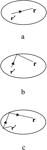
Figure 1: Schematic representation of a few classical orbits contributing to the polarization propagator (10) for a finite system. Figure (a) shows the direct trajectory from ${\bf r}^{\prime}$ to ${\bf r}$, this is the only trajectory contributing to the propagator in a collisionless homogeneous system. Figures (b) and (c) show two typical trajectories with one and two reflections at the boundary.

Bertsch [9] used the Vlasov equation as a starting point for a theory of giant resonances in nuclei. He pointed out that, since the Vlasov dynamics preserves the density of points in phase space, it does not violate the Pauli principle, even if it is a completely classical theory. Thus, Eq.(7), after having been used by Jeans for stellar systems, by Vlasov and Landau for plasmas, by Landau for liquid helium and by Kirzhnitz et al. for atoms, found its way into nuclear physics as well.

3 FIXED BOUNDARY

3.1 Integrable systems

The expression (10) for $\Pi^{0}({\bf r},{\bf r}^{\prime},\omega)$ is quite general and in principle it is valid also for systems in which the motion of particles in the equilibrium mean field is chaotic, however it is not really suitable for practical calculations since evaluating the time integral requires following the particle trajectories over an infinite time interval. Kirzhnitz et al. avoided this difficulty by restricting themselves to systems in which the particle motion is periodic, but this is a very severe limitation. In the more recent work of Brink et al. [10] it has been shown that there is an important class of finite systems for which the solution of the linearized Vlasov equation acquires a relatively simple form: they are all the systems for which the motion of particles in the equilibrium mean field can be described by an integrable Hamiltonian, this includes for example all spherically symmetric systems, but also some deformed systems. In these systems the particle motion is multiply periodic and, as a consequence, it is sufficient to follow the particle motion only over a finite time interval. The crucial step in applying the approach of [6] to integrable systems, is an appropriate change of variables. The $({\bf r},{\bf p})$ variables are convenient for translation-invariant systems, since in that case ${\partial V_{0}}/{\partial{\bf r}}=0$ and the linearized version of Eq. (7) becomes simpler. A similar simplification can be obtained for integrable systems if action-angle variables $({\bf I},{\bf\Phi})$ are used instead of $({\bf r},{\bf p})$. For these systems the action variables $I_{\alpha}$ are constants of the motion, while the conjugate angle variables $\Phi_{\alpha}$ are linear functions of time (see for example Ref. [11], p. 457). An important property of these variables is that the motion is periodic in the angle variables with period $2\pi$. Consequently the field felt by a particle that is moving along such a trajectory can be Fourier expanded as

$$V_{ext}({\bf r},\omega)=\beta(\omega)\sum_{{\bf n}}Q_{\bf n}({\bf I})e^{i{\bf n}\cdot{\bf\Phi}}\,,$$ (12)

where ${\bf n}$ is a three-dimensional vector with integer components. Similar expansions hold also for the fluctuations of the mean field

$$\delta V({\bf r},\omega)=\sum_{{\bf n}}\delta V_{\bf n}({\bf I},\omega)e^{i{\bf n}\cdot{\bf\Phi}}$$ (13)

and of the distribution function

$$\delta f({\bf r},{\bf p},\omega)=\sum_{\bf n}\delta f_{\bf n}({\bf I},\omega)e^{i{\bf n}\cdot{\bf\Phi}}\,.$$ (14)

When Eq.(7) is Fourier transformed in time and linearized by neglecting terms of order $(\delta f)^{2}$ and higher, it reads

$$-i\omega\delta f(\omega)+\{\delta f,h_{0}\}$$ (15)

$$+F^{\prime}(h_{0})\{h_{0},[V^{ext}(\omega)+\delta V(\omega)]\}=0\,.$$

Here the braces denote Poisson brackets, that can be evaluated according to any set of canonically conjugate variables, using ${\bf r}$ and ${\bf p}$ gives the linearized version of Eq.(7), while using ${\bf I}$ and ${\bf\Phi}$ gives

$$-i\omega\delta f(\omega)+\kern-0.24994pt\hbox{$\omega$}\kern-6.22453pt\kern 0.50003pt\hbox{$\omega$}\kern-6.22453pt\kern-0.24994pt\raise 0.43304pt\hbox{$\omega$}\cdot\frac{\partial\delta f}{\partial{\bf\Phi}}=$$ (16)

$$F^{\prime}(h_{0})\,\kern-0.24994pt\hbox{$\omega$}\kern-6.22453pt\kern 0.50003pt\hbox{$\omega$}\kern-6.22453pt\kern-0.24994pt\raise 0.43304pt\hbox{$\omega$}\cdot{\Big{(}}\frac{\partial V^{ext}}{\partial{\bf\Phi}}+\frac{\partial\delta V}{\partial{\bf\Phi}}{\Big{)}}\,.$$

The three components of the vector $\omega$$\omega$$\omega$ determine the time-dependence of the angle variables:

$$\dot{\Phi}_{\alpha}=\frac{\partial h_{0}({\bf I},{\bf\Phi})}{\partial I_{\alpha}}=\omega_{\alpha}\,,$$ (17)

while, of course

$$\dot{I}_{\alpha}=-\frac{\partial h_{0}({\bf I},{\bf\Phi})}{\partial\Phi_{\alpha}}=0\,,$$ (18)

and $h_{0}=h_{0}({\bf I})$.

By using the expansions (12-14), Eq.(16) gives

$$\delta f_{\bf n}({\bf I},\omega)=F^{\prime}(h_{0}){\Big{[}}\beta(\omega)Q_{\bf n}({\bf I})$$ (19)

$$+\delta V_{\bf n}({\bf I},\omega){\Big{]}}\frac{{\bf n}\cdot{\kern-0.24994pt\hbox{$\omega$}\kern-6.22453pt\kern 0.50003pt\hbox{$\omega$}\kern-6.22453pt\kern-0.24994pt\raise 0.43304pt\hbox{$\omega$}}}{{\bf n}\cdot{\kern-0.24994pt\hbox{$\omega$}\kern-6.22453pt\kern 0.50003pt\hbox{$\omega$}\kern-6.22453pt\kern-0.24994pt\raise 0.43304pt\hbox{$\omega$}}-(\omega+i\varepsilon)}\,.$$

We have added a vanishingly small positive imaginary part $i\varepsilon$ in order to specify the behaviour of $\delta f_{\bf n}(\omega)$ at the pole .

Equation (19) gives an explicit solution of the linearized Vlasov equation only if the fluctuation of the mean field $\delta V$ can be neglected, otherwise it gives only an implicit solution, since $\delta V$ does depend on $\delta f$; however its form immediately suggests an iterative procedure for obtaining the full solution: first evaluate $\delta f^{0}$ by neglecting $\delta V$ in (19), then evaluate $\delta V$ by using $\delta f^{0}$ as input and repeat until convergence is obtained.

The quantity $\delta f$ is not very convenient for discussing the solution of the linearized Vlasov equation, since it depends on the external driving force, so it is appropriate to introduce the polarization propagators (9) and (10) , whose properties depend only on the system. Clearly, once we know $\delta f$, by using Eqs. (1) and (11), we can obtain a corresponding expression for the propagators $\Pi^{0}$ and $\Pi$. We prefer to use their momentum representations, obtained from (9) and (10) by taking Fourier transforms with respect to the coordinates:

$$\Pi({\bf q},{\bf q}^{\prime},\omega)=\int d{\bf r}\int d{\bf r}^{\prime}e^{-i{\bf q}\cdot{\bf r}}\Pi({\bf r},{\bf r}^{\prime},\omega)e^{i{\bf q}^{\prime}\cdot{\bf r}^{\prime}}\,.$$ (20)

The expression of the $\Pi^{0}$ propagator is [13]

$$\Pi{{}^{0}}({\bf q}^{\prime},{\bf q},\omega)=$$ (21)

$$(2\pi)^{3}\sum_{\bf n}\int d{\bf I}\,F^{\prime}(h_{0}({\bf I}))$$

$$\times\frac{{\bf n}\cdot{\kern-0.24994pt\hbox{$\omega$}\kern-6.22453pt\kern 0.50003pt\hbox{$\omega$}\kern-6.22453pt\kern-0.24994pt\raise 0.43304pt\hbox{$\omega$}}({\bf I})}{{\bf n}\cdot{\kern-0.24994pt\hbox{$\omega$}\kern-6.22453pt\kern 0.50003pt\hbox{$\omega$}\kern-6.22453pt\kern-0.24994pt\raise 0.43304pt\hbox{$\omega$}}({\bf I})-(\omega+i\varepsilon)}\,Q^{*}_{\bf n}({\bf q}^{\prime},{\bf I})~{}Q_{\bf n}({\bf q,I})\,,$$

with the Fourier coefficients

$$Q_{\bf n}({\bf q,I})=\frac{1}{(2\pi)^{3}}\int d\kern-0.24994pt\hbox{$\Phi$}\kern-7.22223pt\kern 0.50003pt\hbox{$\Phi$}\kern-7.22223pt\kern-0.24994pt\raise 0.43304pt\hbox{$\Phi$}\,e^{-i{\bf n}\cdot{\kern-0.17496pt\hbox{$\Phi$}\kern-5.05556pt\kern 0.35002pt\hbox{$\Phi$}\kern-5.05556pt\kern-0.17496pt\raise 0.30313pt\hbox{$\Phi$}}}\,e^{i{\bf q}\cdot{\bf r}}\,.$$ (22)

If the interaction $v({\bf x},{\bf y})$ does depend only on the distance between particles, the integral equation (9) becomes [14]

$$\Pi({\bf q}^{\prime},{\bf q},\omega)=\Pi^{0}({\bf q}^{\prime},{\bf q},\omega)$$ (23)

$$+\frac{1}{(2\pi)^{3}}\int d{\bf k}\,\Pi^{0}({\bf q}^{\prime},{\bf k},\omega)\,v(k)\,\Pi({\bf k},{\bf q},\omega)\,.$$

3.2 Spherical systems

Spherical systems are an important class of integrable systems, hence they deserve a more detailed discussion. Actually these systems are over-integrable, since in this case there are four constants of motion (the particle enegy $\epsilon$ and the three components of its angular momentum $\kern-0.24994pt\hbox{$\lambda$}\kern-5.83336pt\kern 0.50003pt\hbox{$\lambda$}\kern-5.83336pt\kern-0.24994pt\raise 0.43304pt\hbox{$\lambda$}={\bf r}\times{\bf p})$, so one of the angle variables must also be constant. The action-angle variables $({\bf I},{\bf\Phi})$ allow for a very compact solution of the linearized Vlasov equation (15), but they are not the only set of variables that can simplify the problem. The important point is to choose as variables the largest possible number of constants of motion, so that the number of partial derivatives in Eq.(15) can be reduced.

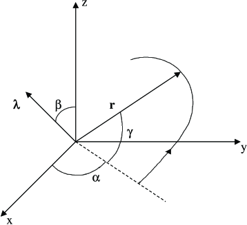
Figure 2: Angular elements of the orbit. For a particle moving in a central force field, the angles $\alpha$ and $\beta$ are constant.

The variables used in [10] instead of $({\bf r},{\bf p})$ are $(\epsilon,\lambda,r,\alpha,\beta,\gamma)$ of which four ($\epsilon$, $\lambda$, and the two angles $\alpha$ and $\beta$ shown in Fig.2) are constants of motion. So we are left only with the two partial derivatives with respect to $r$ and $\gamma$ in Eq.(15). The $\gamma$-derivative can be eliminated by means of the expansion

$$\delta f({\bf r},{\bf p},\omega)=\sum_{LM}\delta f_{LM}(r,{\bf p},\omega)Y_{LM}(\theta,\varphi)$$ (24)

and by using the well-known transformation property of the spherical harmonics $Y_{LM}(\theta,\varphi)$ under the rotation specified by the Euler angles $(\alpha,\beta,\gamma)$ (see e. g. [15], p. 28):

$$Y_{LM}(\theta,\varphi)=\sum_{N}{\Big{(}}{\mathcal{D}}^{L}_{MN}(\alpha,\beta,\gamma){\Big{)}}^{*}Y_{LN}(\theta^{\prime},\varphi^{\prime})\,.$$ (25)

If the new reference frame rotates with the particle, the angles $\theta^{\prime}$ and $\varphi^{\prime}$ are constant and the only time-dependent angle is $\gamma$. The quantities ${\mathcal{D}}^{L}_{MN}(\alpha,\beta,\gamma)$ are the rotation matrices and their explicit $\gamma$-dependence, of the kind $e^{-iN\gamma}$, can be exploited to eliminate the $\gamma$-derivative. In this way the initial three-dimensional problem is reduced to a one-dimensional problem for particles moving in the effective potential $V_{eff}=V_{0}(r)+\frac{\lambda^{2}}{2mr^{2}}$.

Then, as shown in [10], the expansion (24) can be written as

$$\delta f({\bf r},{\bf p},\omega)=$$ (26)

$$\sum_{LMN}{\Big{[}}\delta f^{L+}_{MN}(\epsilon,\lambda,r,\omega)+\delta f^{L-}_{MN}(\epsilon,\lambda,r,\omega){\Big{]}}$$

$$\times{\Big{(}}{\mathcal{D}}^{L}_{MN}(\alpha,\beta,\gamma){\Big{)}}^{*}Y_{LN}(\frac{\pi}{2},\frac{\pi}{2})\,.$$

The functions $\delta f^{L\pm}_{MN}$ refer to particles having positive $(\delta f^{L+}_{MN})$ or negative $(\delta f^{L-}_{MN})$ components of the radial velocity, of magnitude $v_{r}(\epsilon,\lambda,r)=\sqrt{\frac{2}{m}(\epsilon-V_{eff})}$.

The linearized Vlasov equation (15) implies the following system of coupled first-order differential equations in the variable $r$ for the functions $\delta f^{L\pm}_{MN}$

$$\frac{\partial}{\partial r}\delta f^{L\pm}_{MN}\mp A_{N}\delta f^{L\pm}_{MN}=B^{L\pm}_{MN}\,,$$ (27)

with

$$A_{N}(\epsilon,\lambda,r,\omega)=\frac{i\omega}{v_{r}(\epsilon,\lambda,r)}-\frac{iN}{v_{r}(\epsilon,\lambda,r)}\frac{\lambda}{mr^{2}}$$ (28)

and

$$B^{L\pm}_{MN}(\epsilon,\lambda,r,\omega)=$$ (29)

$$F^{\prime}(\epsilon){\Big{(}}\frac{\partial}{\partial r}\pm\frac{iN}{v_{r}(\epsilon,\lambda,r)}\frac{\lambda}{mr^{2}}{\Big{)}}$$

$${\Big{[}}\beta(\omega)Q_{LM}(r)+\delta V_{LM}(r,\omega){\Big{]}}\,.$$

The functions $Q_{LM}(r)$ and $\delta V_{LM}(r,\omega)$ are the coefficients of a multipole expansion similar to (24) for the external driving field and for the induced mean-field fluctuations, respectively. Because of Eq.(4), the term $\delta V_{LM}(r,\omega)$ couples the two equations (27) for $\delta f^{L+}_{MN}$ and $\delta f^{L-}_{MN}$:

$$\delta V_{LM}(r,\omega)=$$ (30)

$$\frac{8\pi^{2}}{2L+1}\sum_{N=-L}^{L}{\Big{|}}Y_{LN}(\frac{\pi}{2},\frac{\pi}{2}){\Big{|}}^{2}$$

$$\int d\epsilon\int d\lambda\lambda\int\frac{dr^{\prime}}{v_{r}(r^{\prime})}v_{L}(r,r^{\prime})$$

$${\big{[}}\delta f^{L+}_{MN}(\epsilon,\lambda,r^{\prime},\omega)+\delta f^{L-}_{MN}(\epsilon,\lambda,r^{\prime},\omega){\big{]}}\,.$$

Before solving the system of equations (27), we must specify the boundary conditions satisfied by the phase-space density fluctuations. The conditions used in [10] are

$$\delta f^{L+}_{MN}(r_{1})=\delta f^{L-}_{MN}(r_{1})\,,$$ (31)

$$\delta f^{L+}_{MN}(r_{2})=\delta f^{L-}_{MN}(r_{2})\,,$$ (32)

where $r_{1(2)}$ are the classical turning points, for which $v_{r}(\epsilon,\lambda,r)=0$.

With these boundary conditions the solution of the linearized Vlasov equation for spherical systems agrees with that given by the method of action-angle variables [10].

There are some some further simplifications for the polarization propagators of spherical systems, compared to those given in the previous subsection. The three-dimensional integral equation (23) reduces to a set of one-dimensional integral equations for each multipolarity $L$

$$\Pi_{L}(q^{\prime},q,\omega)=\Pi^{0}_{L}(q^{\prime},q,\omega)+\frac{1}{(2\pi)^{3}}$$ (33)

$$\int_{0}^{\infty}dkk^{2}\,\Pi^{0}_{L}(q^{\prime},k,\omega)\,v(k)\,\Pi_{L}(k,q,\omega)\,,$$

and the $\Pi^{0}$ propagator also becomes somewhat simpler than (21):

$$\Pi^{0}_{L}(q^{\prime},q,\omega)=$$ (34)

$$\frac{8\pi^{2}}{2L+1}\sum_{n=-\infty}^{+\infty}\sum_{N=-L}^{L}{\Big{|}}Y_{LN}(\frac{\pi}{2}\frac{\pi}{2}){\Big{|}}^{2}$$

$$\int d\epsilon F^{\prime}(\epsilon)\int d\lambda\,\lambda\,T\frac{n\omega_{0}+N\omega_{\varphi}}{n\omega_{0}+N\omega_{\varphi}-(\omega+i\varepsilon)}$$

$$Q^{(L)\,*}_{nN}(q^{\prime},\epsilon,\lambda)Q^{(L)}_{nN}(q,\epsilon,\lambda)\,.$$

Here $\omega_{0}(\epsilon,\lambda)$ is the frequency of radial motion of a particle with enegy $\epsilon$ and magnitude of angular momentum $\lambda$ in the effective potential $V_{eff}$, while $\omega_{\varphi}(\epsilon,\lambda)$ is the precession frequency of the periapsis in the plane of the orbit ([11],p.509). These two frequencies determine the shape of the orbit in a central potential. The period of radial motion $T$ is $T(\epsilon,\lambda)=2\pi/\omega_{0}$. The Fourier coefficients $Q^{(L)}_{nN}(q,\epsilon,\lambda)$ are given by

$$Q^{(L)}_{nN}(q,\epsilon,\lambda)=$$ (35)

$$\frac{2}{T}\int_{r_{1}}^{r_{2}}\frac{dr}{v_{r}(\epsilon,\lambda,r)}\cos[s_{nN}(r)]\,Q_{L}(qr)\,,$$

with

$$Q_{L}(qr)=4\pi i^{L}j_{L}(qr)\,.$$ (36)

The phases $s_{nN}(r)$ are

$$s_{nN}(r)=n\omega_{0}\tau(r)+N{\big{(}}\omega_{\varphi}\tau(r)-\gamma(r){\big{)}}\,,$$ (37)

where

$$\tau(r)=\int_{r_{1}}^{r}\frac{dr^{\prime}}{v_{r}(\epsilon,\lambda,r^{\prime})}\,,$$ (38)

is the time taken by a particle to move from the inner turning point $r_{1}$ to point $r$, and

$$\gamma(r)=\int_{r_{1}}^{r}\frac{dr^{\prime}}{v_{r}(\epsilon,\lambda,r^{\prime})}\frac{\lambda}{mr^{\prime 2}}$$ (39)

is the angle spanned by the radius vector during the time interval $\tau(r)$.

In Eqs. (21) and (34) it has been asumed that the equilibrium distribution of particles depends only on the particle energy. Usually one takes $F(\epsilon)\propto\theta(\epsilon_{F}-\epsilon)$,where $\epsilon_{F}$ is the Fermi energy, so that $F^{\prime}(\epsilon)\propto\delta(\epsilon_{F}-\epsilon)$ and the expression (34) becomes simpler.

At first sight it might seem that the infinite sum over $n$ in (34) might create difficulties, but in practice it is enough to include in the sum the very first few terms around $n=0$ to get a sufficient approximation.

3.3 Atomic plasmons?

The early calculations of Kirzhnitz and collaborators suggested the existence of two collective high-energy excitations in the spectrum of heavy atoms [6]. These excitations had been interpreted as collective, plasmon-type oscillations of the atomic electron cloud. In order to apply their formalism, Kirzhnitz et al. had to approximate the atomic self-consistent mean field with a potential in which electrons having zero total energy move along closed trajectories. Our closely related approach allows also for orbits that are not closed, but, of course, it can be applied also to closed trajectories. This has been done in [16], where the calculations of Kirzhnitz et al. have been repeated by using the formalism discussed in this Section. In that study only one “collective” solution of the integral equation (33) was found,moreover, thanks to the analytical insight given by the semiclassical method, this solution was shown to be qualitatively different from the plasma oscillations of a uniform electron gas. While plasma oscillations belong to a strong-coupling regime (see e.g. [17], p. 185), the “collective” solution found in [16] pertains to a regime of weak coupling. Thus it was concluded that there is no evidence for plasmon-like excitations in this semiclassical theory of atomic spectra. This conclusion is in agreement with the result of analogous quantum calculations.

3.4 Integrable spheroidal systems

The equilibrium self-consistent mean field in heavy closed-shell nuclei is well approximated by a spherical Saxon-Woods potential, with parameters that can be determined phenomenologically. A somewhat similar mean field describes also metal clusters [18]. Thus,

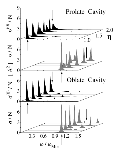
Figure 3: Photoabsorption cross section per valence electron (shaded grey) for prolate and oblate sodium clusters. The black-shaded peaks show results obtained in the single-particle approximation in which the mean-field fluctuation (4) is neglected. The arrows indicate the position of the plasmon peak in the spherical case.

for open-shell systems it is reasonable to try a deformed Saxon-Woods like potential. However the results of the first subsection cannot be applied to this kind of potentials, since accurate calculations of the classical phase space for axially deformed Saxon-Woods potentials have shown that it contains regions of chaoticity [19]. But, if the surface diffuseness is neglected and a spheroidal cavity is assumed to approximate the mean field of large deformed nuclei [20] or clusters, then that formalism can be applied directly. This has been done in Ref. [21] to study the surface plasmons in deformed atomic clusters. The main result of that paper is that, under certain conditions, oblate deformed clusters may display a more complex shape of the surface plasmon peaks than predicted by the classical Mie theory (three peaks instead of two). This prediction has not yet been checked experimentally.

Fig. 3 shows essentially the single-particle (shaded black) and collective (shaded grey) dipole strength functions for prolate and oblate spheroidal clusters. The figure is taken from Ref. [21]. The deformation parameter $\eta$ is the ratio between the larger and smaller radius of the spheroid. The frequency is expressed in units of the Mie frequency $\omega_{Mie}$. In the lower panel the fragmentation of the high-frequency peak is clearly visible for deformations $\eta=1.25$ and $\eta=1.5$.

4 MOVING
BOUNDARY

4.1 Connection with liquid drop model

In heavy closed-shell nuclei the equilibrium mean field can be further approximated by a spherical square-well potential of radius $R\approx 1.2A^{\frac{1}{3}}{\rm fm}$. In this simplified picture several of the quantities needed to evaluate the linear response of the system can be expressed analytically, hence it gives a useful reference model.

When the surface diffusion is neglected, the boundary condition (32) corresponds to requiring that the particles collide elastically with the static nuclear surface $r_{2}=R$ (mirror-reflection condition).

In Ref. [22] it has been shown that the results of [10] can be generalized to a model in which the sharp surface is allowed to vibrate, simply by changing the boundary condition (32).

If the radius of a spherical nucleus is allowed to vibrate according to the usual liquid-drop model expression [23]

$$R(\theta,\varphi,t)=R+\sum_{LM}\delta R_{LM}(t)Y_{LM}(\theta,\varphi)\,,$$ (40)

then the mirror-reflection condition (32) is changed to

$$\delta\tilde{f}^{L+}_{MN}(R)-\delta\tilde{f}^{L-}_{MN}(R)=2F^{\prime}(\epsilon)i\omega p_{r}\delta R_{LM}(\omega)\,,$$ (41)

where $p_{r}$ is the magnitude of the radial component of the particle momentum. We put a tilde over the moving-surface solutions to distinguish them from the untilded fixed-surface solutions. The boundary condition (41) still corresponds to a mirror reflection, but in the reference frame of the moving surface.

It can be easily checked by direct substitution that the following integral equation

$$\delta\tilde{f}^{L\pm}_{MN}(\epsilon,\lambda,r,\omega)=$$ (42)

$$F^{\prime}(\epsilon)\frac{e^{\pm i[\omega\tau(r)-N\gamma(r)]}}{\sin[\omega\tau(R)-N\gamma(R)]}\omega p_{r}\delta R_{LM}(\omega)$$

$$+{\big{\{}}\int_{r_{1}}^{r}dr^{\prime}\tilde{B}^{L\pm}_{MN}(\epsilon,\lambda\,r^{\prime})e^{\mp[i\omega\tau(r^{\prime})-N\gamma(r^{\prime})]}$$

$$+\tilde{C}^{L}_{MN}(\epsilon,\lambda,\omega){\big{\}}}e^{\pm i[\omega\tau(r)-N\gamma(r)]}\,,$$

with

$$\tilde{B}^{L\pm}_{MN}(\epsilon,\lambda,r,\omega)=$$ (43)

$$F^{\prime}(\epsilon){\Big{(}}\frac{\partial}{\partial r}\pm\frac{iN}{v_{r}(\epsilon,\lambda,r)}\frac{\lambda}{mr^{2}}{\Big{)}}$$

$${\Big{[}}\beta(\omega)Q_{LM}(r)+\delta\tilde{V}_{LM}(r,\omega){\Big{]}}\,,$$

$$\delta\tilde{V}_{LM}(r,\omega)=$$ (44)

$$\frac{8\pi^{2}}{2L+1}\sum_{N=-L}^{L}{\Big{|}}Y_{LN}(\frac{\pi}{2},\frac{\pi}{2}){\Big{|}}^{2}$$

$$\int d\epsilon\int d\lambda\lambda\int\frac{dr^{\prime}}{v_{r}(r^{\prime})}v_{L}(r,r^{\prime})$$

$${\big{[}}\delta\tilde{f}^{L+}_{MN}(\epsilon,\lambda,r^{\prime},\omega)+\delta\tilde{f}^{L-}_{MN}(\epsilon,\lambda,r^{\prime},\omega){\big{]}}$$

and

$$\tilde{C}^{L}_{MN}(\epsilon,\lambda,\omega)=$$ (45)

$${\Big{\{}}e^{i2[\omega\tau(R)-N\gamma(R)]}$$

$$\int_{r_{1}}^{R}dr\tilde{B}^{L+}_{MN}(\epsilon,\lambda,r)e^{-i[\omega\tau(r)-N\gamma(r)]}$$

$$-\int_{r_{1}}^{R}dr\tilde{B}^{L-}_{MN}(\epsilon,\lambda,r)e^{i[\omega\tau(r)-N\gamma(r)]}{\Big{\}}}$$

$$\times{\Big{\{}}1-e^{i2[\omega\tau(R)-N\gamma(R)]}{\Big{\}}}^{-1}$$

is equivalent to the system

$$\frac{\partial}{\partial r}\delta\tilde{f}^{L\pm}_{MN}\mp A_{N}\delta\tilde{f}^{L\pm}_{MN}=\tilde{B}^{L\pm}_{MN}$$ (46)

with the boundary conditions (31) and (41), and that it respects the self-consistency condition (4).

Equations (42-45) give an implicit solution of the linearized Vlasov equation with moving-surface boundary conditions. They are more complicated than the corresponding fixed-surface equations because they contain also the unknown collective coordinates $\delta R_{LM}(\omega)$. In order to proceed further, we need an additional relation that specifies these quantities. As shown in [22], this relation can be found within the liquid-drop model if one recalls that, in that model, a change in the curvature radius of the surface results in a change of the pressure at the surface given by (cf. Eq. (6A-57) of [23])

$$\delta{\cal P}(R,\theta,\varphi,\omega)=\sum_{LM}C_{L}\frac{\delta R_{LM}(\omega)}{R^{4}}Y_{LM}(\theta,\varphi)\,.$$ (47)

The restoring force parameter $C_{L}$ can be easily evaluated: if the Coulomb repulsion between protons is neglected,

$$C_{L}=\sigma R^{2}(L-1)(L+2)\,,$$ (48)

where $\sigma\approx 1{\rm MeV\,fm}^{-2}$ is the phenomenological surface-tension parameter, while taking into account also the Coulomb interaction changes somewhat this expression [23].

The connection with kinetic theory is then made simply by noticing that the surface pressure (47) is an appropriate diagonal element of the tensor (2) (generalized to Fermi liquids, see e. g. [24]):

$$\delta{\cal P}(R,\theta,\varphi,\omega)=\lim_{r\to R}$$ (49)

$$\int d{\bf p}p_{r}v_{r}{\big{(}}\delta\tilde{f}({\bf r},{\bf p},\omega)-F^{\prime}(\epsilon)\delta\tilde{V}({\bf r},\omega){\big{)}}\,.$$

This integral must be evaluated for $r<R$ and then we must let $r\to R$ from inside.

Multiplying both (47) and (49) by $Y_{LM}^{*}(\theta,\varphi)$ and integrating over the directions of ${\bf r}$, gives

$$\delta R_{LM}(\omega)=$$ (50)

$$\frac{8\pi^{2}}{2L+1}\frac{R^{2}}{C_{L}}\sum_{N=-L}^{L}{\Big{|}}Y_{LN}(\frac{\pi}{2},\frac{\pi}{2}){\Big{|}}^{2}$$

$$\int d\epsilon\int d\lambda\lambda p_{r}{\Big{[}}\delta\tilde{f}^{L}_{MN}(\epsilon,\lambda,R,\omega)$$

$$-2F^{\prime}(\epsilon)\delta\tilde{V}_{LM}(R,\omega){\Big{]}}\,,$$

with the definition

$$\delta\tilde{f}^{L}_{MN}\equiv\delta\tilde{f}^{L+}_{MN}+\delta\tilde{f}^{L-}_{MN}\,.$$ (51)

Equation (50) relates the fluctuations of surface and distribution-function in the approach of [22]; it is an implicit relation for $\delta R$, since both $\delta\tilde{f}$ and $\delta\tilde{V}$ do depend on $\delta R$.

4.2 Approximate solutions for surface vibrations

In order to obtain an explicit expression for the collective coordinates $\delta R_{LM}(\omega)$ we make the following approximation:

$$\delta\tilde{f}^{L}_{MN}(\epsilon,\lambda,r,\omega)=\delta f^{L}_{MN}(\epsilon,\lambda,r,\omega)$$ (52)

$$+2F^{\prime}(\epsilon)\frac{\cos[\omega\tau(r)-N\gamma(r)]}{\sin[\omega\tau(R)-N\gamma(R)]}\omega p_{r}\delta R_{LM}(\omega)\,,$$

with $\delta{f}^{L}_{MN}(\epsilon,\lambda,r,\omega)$ the fixed-surface solution. This approximation is based on the assumption that, apart from the term proportional to $\delta R_{LM}$, which alone fulfills the boundary condition (41), in the bulk of the system the moving-surface solution does not differ too much from the fixed-surface one.

Then, Eq. (50) gives:

$$\delta R_{LM}(\omega)=$$ (53)

$${\Big{\{}}\frac{8\pi^{2}}{2L+1}\sum_{N=-L}^{L}{\Big{|}}Y_{LN}(\frac{\pi}{2},\frac{\pi}{2}){\Big{|}}^{2}$$

$$\int d\epsilon\int d\lambda\lambda p_{r}{\Big{[}}\delta f^{L}_{MN}(\epsilon,\lambda,R,\omega)$$

$$-2F^{\prime}(\epsilon)\delta V_{LM}(R,\omega){\Big{]}}{\Big{\}}}{\Big{\{}}\frac{C_{L}}{R^{2}}$$

$$-\frac{(4\pi)^{2}}{2L+1}\sum_{N=-L}^{L}{\Big{|}}Y_{LN}(\frac{\pi}{2},\frac{\pi}{2}){\Big{|}}^{2}\int d\epsilon F^{\prime}(\epsilon)$$

$$\int d\lambda\lambda p_{r}{\Big{[}}\omega p_{r}\cot[\omega\tau(R)-N\gamma(R)]-$$

$$\alpha_{L}(R,\omega){\Big{]}}{\Big{\}}}^{-1}\,,$$

with

$$\alpha_{L}(r,\omega)=$$ (54)

$$\frac{(4\pi)^{2}}{2L+1}m\sum_{N=-L}^{L}{\Big{|}}Y_{LN}(\frac{\pi}{2},\frac{\pi}{2}){\Big{|}}^{2}$$

$$\int d\epsilon F^{\prime}(\epsilon)\int d\lambda\lambda\int dr^{\prime}v_{L}(r,r^{\prime})\,$$

$$\frac{\cos[\omega\tau(r^{\prime})-N\gamma(r^{\prime})]}{\sin[\omega\tau(R)-N\gamma(R)]}\omega\,.$$

Equation (53) is an interesting, although approximate, expression for the collective coordinates given by the approach of Ref. [22]. The vanishing of the denominator in this expression determines the poles of $\delta R_{LM}(\omega)$, hence the eigenfrequencies of the surface vibrations $\delta R_{LM}(t)$. Note that, according to Eq. (53), for $L\neq 1$ these eigenfrequencies depend on the surface tension, which is physically sound.

The eigenfrequencies determined by the vanishing of the denominator in Eq. (53) can be directly compared to the experimental excitation energies of the corresponding modes. Up to now this has been done only after making an additional approximation: if the fixed-surface solution is approximated by its zero-order expression $\delta f^{0\,L}_{MN}$, appropriate for a gas of non-interacting particles, a corresponding zero-order approximation is obtained for $\delta R_{LM}(\omega)$

$$\delta R^{0}_{LM}(\omega)=$$ (55)

$${\Big{\{}}\frac{8\pi^{2}}{2L+1}\sum_{N=-L}^{L}{\Big{|}}Y_{LN}(\frac{\pi}{2},\frac{\pi}{2}){\Big{|}}^{2}$$

$$\int d\epsilon\int d\lambda\lambda p_{r}{\Big{[}}\delta f^{0\,L}_{MN}(\epsilon,\lambda,R,\omega){\Big{]}}{\Big{\}}}{\Big{\{}}\frac{C_{L}}{R^{2}}$$

$$-\frac{(4\pi)^{2}}{2L+1}\sum_{N=-L}^{L}{\Big{|}}Y_{LN}(\frac{\pi}{2},\frac{\pi}{2}){\Big{|}}^{2}\omega\int d\epsilon F^{\prime}(\epsilon)$$

$$\int d\lambda\lambda p^{2}_{r}{\Big{[}}\cot[\omega\tau(R)-N\gamma(R)]{\Big{]}}{\Big{\}}}^{-1}\,.$$

Note that this approximation contains more dynamics than the corresponding fixed-surface zero-order approximation, since the interaction between particles is taken into account to some extent through the phenomenological surface-tension parameter $\sigma$.

4.3 Surface and compression modes

It is interesting to compare the dynamics described by Eq. (55) with that of the liquid-drop model.

The vanishing of the denominator in Eq. (55) can be written as

$$\frac{C_{L}}{R^{2}}-\frac{\chi_{L}(\omega)}{R^{2}}=0\,,$$ (56)

with the function $\chi_{L}(\omega)$ defined as in Ref. [25]:

$$\chi_{L}(\omega)=$$ (57)

$$\omega R^{2}\frac{(4\pi)^{2}}{2L+1}\sum_{N=-L}^{L}{\Big{|}}Y_{LN}(\frac{\pi}{2},\frac{\pi}{2}){\Big{|}}^{2}$$

$$\int d\epsilon F^{\prime}(\epsilon)\int d\lambda\lambda p^{2}_{r}\cot[\omega\tau(R)-N\gamma(R)]\,.$$

The expression analogous to (56) in the liquid-drop model is

$$C_{L}-\omega^{2}D_{L}=0\,,$$ (58)

or, allowing also for compression modes (cf. Eq. (6A-58) of [23]),

$$C_{L}-\omega^{2}D_{L}\,{L\over R}\,{{j_{L}({\omega\over u_{c}}R)}\over{\partial\over\partial r}j_{L}({\omega\over u_{c}}r)\mid_{r=R}}=0\,,$$ (59)

with $u_{c}$ the velocity of sound. This condition determines the eigenfrequencies of the various modes in the liquid-drop model [23]. These eigenfrequencies depend also on the mass parameters $D_{L}$ that can be evaluated within that model, but one has to make some assumption about the kind of flow occurring in the system [23].

In order to make a comparison between the solutions of (56) and (59) it would be desirable to have a simple analytical expression for the function $\chi_{L}(\omega)$. The pole expansion of the cotangent

$$\cot z=\sum^{\infty}_{n=-\infty}\frac{1}{z-n\pi}$$ (60)

allows us to express $\chi_{L}(\omega)$ in a form that is more similar to the $\Pi^{0}_{L}$ propagator (34):

$$\chi_{L}(\omega)=\omega R^{2}\frac{(16\pi)}{2L+1}$$ (61)

$$\sum_{n=-\infty}^{\infty}\sum_{N=-L}^{L}{\Big{|}}Y_{LN}(\frac{\pi}{2},\frac{\pi}{2}){\Big{|}}^{2}\int d\epsilon F^{\prime}(\epsilon)$$

$$\int d\lambda\lambda p^{2}_{r}\frac{\omega_{0}}{(\omega+i\varepsilon)-(n\omega_{0}+N\omega_{\varphi})}\,,$$

but this only shows that $\chi_{L}(\omega)$ is a rather involved complex function. The very fact that $\chi_{L}$ is complex is already an interesting result since we can expect complex eigenfrequencies as solutions of Eq. (56), in close analogy with the Landau damping phenomenon in homogeneous system and in contrast to the liquid-drop model condition (59) that involves only real quantities.

In the case $L=0$ the function $\chi_{L}(\omega)$ can be evaluated analytically [22], while for $L=1,2,3$ relatively simple expressions have been obtained for the coefficients of the low-frequency expansion

$$\chi_{L}(\omega)\approx A_{L}+i\omega\gamma_{L}+D_{L}\omega^{2}\,.$$ (62)

For isoscalar monopole vibrations, the solution of Eq.(56) compares reasonably well with the experimental value of the monopole giant resonance energy in heavy nuclei.

For isoscalar quadrupole oscillations, in [25] it was concluded that the approximation (55) is not adequate to describe the low-energy isoscalar quadrupole excitations. It is not clear if this failure is due to the neglect of the bulk mean-field fluctuations in (55) or to some other reason. Further work is needed on this problem.

About the low-energy isoscalar octupole oscillations, in [25] it was concluded that they are overdamped in the approximation given by Eq. (55), and this might offer a qualitative explanation for the background observed in inelastic proton scattering [26].

Another application of Eq. (55) has been made in Ref. [27]. There this equation has been used to study the isoscalar dipole compression mode. In order to get reasonable results in this case it is vital to treat the centre of mass motion correctly, and this can be done in a fully self-consistent approach. Because Eq.(55) is not really self-consistent, in [27] it was found necessary to add an extra term to the dipole response function based on Eq. (55). For other multipolarities this extra term can also be interpreted as the contribution to the response due to the change of shape of the system in the moving-surface approach, for $L=1$ the system does not change its shape, but can translate as a whole. Since there is no force opposing this translation, this centre of mass motion results in a pole at $\omega=0$ in the dipole response function. The interesting physics is contained in the intrinsic response, that is shown in Fig. 4.

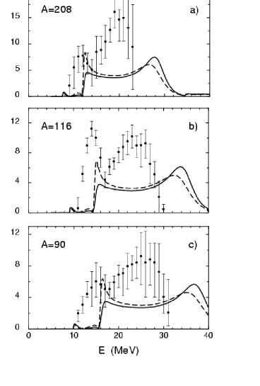
Figure 4: Intrinsic dipole energy-weighted strength function compared to experimental data for ${}^{208}{\rm Pb}$ (a), ${}^{116}{\rm Sn}$ (b) and ${}^{90}{\rm Zr}$ (c). The solid curve is for a confined gas of $A$ non-interacting nucleons with incompressibility $K\approx 200{\rm MeV}$, the dashed curve is for interacting nucleons with $K=160{\rm MeV}$. The data are from Ref.[28]

The results of the moving-surface theory are in qualitative agreement with experimental data on the isoscalar dipole mode, as can be seen from Fig. 4. Moreover, the insight given by this semiclassical approach gives us the possibility to establish a direct link between the peak profile of the isoscalar dipole resonance and the incommpressibility of nuclear matter [27]. This link is evidenced by the dashed curve in Fig. 4.

The approach described here can be easily generalized to a two-component fluid. In [29] such a generalization has been used to study the effect of neutron excess on the isoscalar and isovector monopole response functions. For such a two-component system, Eq.(49) is replaced by the two following equations

$$\delta{\cal P}(R,\theta,\varphi,\omega)=$$ (63)

$$\Pi_{rr}^{n}(R,\theta,\varphi,\omega))+\Pi_{rr}^{p}(R,\theta,\varphi,\omega)\,$$

and

$$\delta{\cal P}_{Q}(R,\theta,\varphi,\omega)=$$ (64)

$$\Pi_{rr}^{n}(R,\theta,\varphi,\omega))-\Pi_{rr}^{p}(R,\theta,\varphi,\omega)\,.$$

Here $\Pi_{rr}^{n(p)}(R,\theta,\varphi,\omega)$ is the normal component of the momentum-flux tensor [r.h.s. of Eq. (49)] associated with neutrons (protons) only. Apart from the usual surface pressure $\delta{\cal P}$ that is present when the neutron and proton surfaces move in phase, in this case there is also an additional pressure $\delta{\cal P}_{Q}$ that is caused by the forces opposing the pulling apart of the neutron and proton surfaces when they move out of phase. This extra pressure can also be related to an appropriate phenomenological parameter. With the surface energy of [30], the pressure $\delta{\cal P}_{Q}$ can be written as

$$\delta{\cal P}_{Q}(R,\theta,\varphi,\omega)=$$ (65)

$${Q\over{2\pi r_{0}^{4}}}\left[\delta R_{n}(\theta,\varphi,\omega)-\delta R_{p}(\theta,\varphi,\omega)\right]\,,$$

where $Q$ is the neutron skin stiffness coefficient of [31] that is analogous to the surface tension parameter $\sigma$ of Eq. (48) and $r_{0}=1.14\,{\rm fm}$.

As shown in [29], the neutron excess does not affect much the isoscalar giant monopole resonance, while its effect on the isovector resonance is more pronounced.

4.4 Fixed vs. moving boundary

The possibility of solving the Vlasov equation with different boundary conditions allows us to decide which condition is more appropriate by comparison with experiment. In Fig. 5 we give an example of a nuclear response function evaluated according to the fixed- and moving-surface boundary conditions.

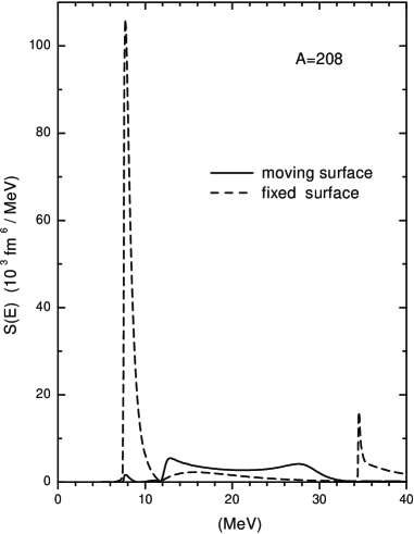
Figure 5: Isoscalar dipole strength functions evaluated in zero-order approximation with moving-surface (full curve) and fixed-surface (dashed curve) boundary conditions. The full curve corresponds to the full curve in Fig.4

In this case there is no doubt that comparison with data (shown in Fig. 4) favours the moving-boundary solution, at least at the level of zero-order approximations. The present example is a rather extreme case, for other response functions the difference between the two solutions is not expected to be so large. Work on detailed comparison between the two solutions for different multipolarities is still in progress.

5 QUANTUM EFFECTS

The Vlasov theory is completely classical, however it is easy to establish a connection with quantum mechanics. It is well known that the time-dependent Hartree-Fock equation for the Wigner transform of the quantal one-body density matrix reads (see e.g. Ref. [32], p. 553)

$$\frac{\partial f({\bf r},{\bf p},t)}{\partial t}+\frac{2}{\hbar}f({\bf r},{\bf p},t)$$ (66)

$$\times\sin[\frac{1}{2}\hbar({\overleftarrow{\bf\nabla}}\cdot{\overrightarrow{\bf\nabla}}_{p}-{\overleftarrow{\bf\nabla}}_{p}\cdot{\overrightarrow{\bf\nabla}})]\>[\frac{p^{2}}{2m}$$

$$+V({\bf r},{\bf p},t)]=0$$

and reduces to

$$\frac{\partial f}{\partial t}+\frac{\bf p}{m}\frac{\partial f}{\partial{\bf r}}$$ (67)

$$-(\frac{\partial V}{\partial{\bf r}})\cdot\frac{\partial f}{\partial{\bf p}}+(\frac{\partial V}{\partial{\bf p}})\cdot\frac{\partial f}{\partial{\bf r}}=0$$

if $\hbar\to 0$. The Hartree-Fock potential $V({\bf r},{\bf p},t)$ is momentum-dependent because the Fock term is non-local in coordinate space. If the momentum-dependence of $V$ is neglected (Hartree approximation), then Eq. (67) coincides with Eq. (7).

There are several possibilities for including quantum effects into the Vlasov theory. The most trivial one is to choose an appropriate equilibrium distribution $F(h_{0}({\bf r},{\bf p}))$. The standard choice for zero-temperature fermions is

$$F(h_{0}({\bf r},{\bf p}))=\frac{g}{(2\pi\hbar)^{3}}\vartheta(\epsilon_{F}-h_{0}({\bf r},{\bf p}))\,,$$ (68)

where $\epsilon_{F}$ is the Fermi enegy and $g$ is the degeneracy factor ($g=2\,(4)$ for electrons (nucleons)).

The choice (68) respects the Pauli principle in the sense that there cannot be more than one fermion of given spin (and isospin) in a phase-space cell of volume $h^{3}$. As stressed by Bertsch [9], the Liouville theorem then ensures that the Pauli principle will be respected during the time evolution of the system described by the Vlasov equation. Thus the Liouville theorem, stating that the points representing the system in the 6-dimensional phase space evolve as an incompressible fluid, justifies the use of the Vlasov equation for quantum systems. Using the equilibrium distribution (68) makes the completey classical Vlasov approach a semiclassical one. Clearly in this way we do not expect to reproduce details, but only gross properties of quantum many-body systems.

In principle one could introduce further quantum effects also by taking into account terms of order $\hbar^{3}$ and higher that have been neglected in Eq. (67). The problem with such a direct approach is that the semiclassical calculations become quickly more complicated than the corresponding quantum calculations, so this method would not be very convenient. A more pragmatic attitude has been taken in Refs. [33] and [13], where the semiclassical propagators given by the Vlasov theory have been compared directly with the analogous quantum propagators.

In [33] the relation between the Fourier coefficients (22) and the corresponding quantum matrix elements has been discussed. If single-particle matrix elements are evaluated in the WKB approximation, they tend to Fourier coefficients analogous to (22) in the limit of large quantum numbers, but this is not necessarily the case for the exact quantum matrix elements.

In [13] the closed-orbit theory, that had been used by various authors to evaluate quantum corrections to the Thomas-Fermi level density, has been applied to evalute quantum corrections to the Vlasov propagator (21). The resulting strength function compares better with the analogous quantum strength function. A fascinating aspect of this study is the possibility of relating features of the excitation spectrum of quantum systems to simple properties of the classical orbits.

6 CONCLUSIONS

In the kinetic-theory approach to linear response discussed here the finite size of the system has been explicitly taken into account. Two different boundary conditions for the density oscillations have been considered: fixed and moving surface.

The fixed-surface solution is closely related to the quantum random phase approximation (RPA) since the integral equation (9) for the semiclassical collective propagator is essentially the same as the equation for the quantum RPA propagator when exchange terms are neglected (Hartree approximation). The main difference between the semiclassical and quantum approaches is in the “free” propagator $\Pi^{0}$. While the quantum expression for this propagator involves wave functions and single-particle energies, the semiclassical propagator involves only properties of the classical orbits and is considerably simpler to evaluate.

The moving-surface solution has been related to the liquid-drop model of nuclei. Compared to that model, the present approach is more microscopic and it allows also for the possibility of Landau damping of collective vibrations.

When compared to experiment, in some cases the semiclassical solutions have the same problems of the RPA and of the liquid-drop model. For example, the fixed-surface approach is, like RPA, able to describe reasonably well the position of the surface plasmon in atomic clusters, but, again like RPA, fails to reproduce the observed width of this resonance. Possible moving-surface contributions to this width have not yet been investigated in detail within the present approach. The moving-surface approach shares with the liquid-drop model the difficulties in reproducing the experimental value of low-energy quadrupole oscillations in heavy nuclei. However the insight given by this approach could be useful for improving both the quantum RPA theory and the liquid-drop model. In conclusion, the semiclassical theory discussed here offers an interesting alternative to the quantum RPA approach because it is simpler to implement numerically, but it is still sufficiently sophisticated to take into account some realistic features (finite size, equilibrium shape) of the many-body system.

References

- [1] Jeans, J.H. 1919, Problems of Cosmology and Stellar Dynamics, Cambridge University Press, Cambridge, UK
- [2] Vlasov, A.A. 1938, Zh. Eksp. Teor. Fiz. 8, 291
- [3] Vlasov, A.A. 1945, J.Phys. U.S.S.R. 9, 25
- [4] Landau, L.D. 1946, J.Phys. U.S.S.R. 10, 25; reprinted in Collected Papers of L.D. Landau, D. Ter Haar (Ed.), Pergamon Press, Oxford, 1960
- [5] Landau, L.D. 1959, Sov. Phys. JETP 5, 101; reprinted in Collected Papers of L.D. Landau, D. Ter Haar (Ed.), Pergamon Press, Oxford, 1960
- [6] Kirzhnitz, D.A., Lozovik, Yu.E., and Shpatakovskaya, G.V. 1975, Sov. Phys. Usp. 18, 649
- [7] Hénon, M. 1982, Astron. Astrophys. 114, 211
- [8] Baym, G., and Pethick, C. 1991, Landau Fermi-Liquid Theory, John Wiley & Sons, Inc., New York
- [9] Bertsch, G.F., 1978, Nuclear Physics with Heavy Ions and Mesons, R. Balian, M. Rho, and G. Ripka (Ed.), North-Holland, Amsterdam, 178
- [10] Brink, D.M., Dellafiore, A., and Di Toro, M. 1986, Nucl. Phys. A456, 205
- [11] Goldstein, H. 1980, Classical Mechanics, 2nd ed., Addison-Wesley Publishing Company, Inc., Reading, Mass.
- [12] Polyachenko, V.L., and Shukhman, I.G., 1981, Sov. Astron. 25, 533
- [13] Dellafiore, A., Matera, F., and Brink, D.M., 1995, Phys. Rev. A 51, 914
- [14] Dellafiore, A., Matera, F. 1990, Phys. Rev. B 41, 3488
- [15] Brink, D.M., and Satchler, G.R. 1968, Angular Momentum, 2nd ed., Clarendon Press, Oxford, UK
- [16] Dellafiore, A., and Matera, F. 1990, Phys. Rev. A 41, 4958
- [17] Fetter, A.L., and Walecka, J.D. 1971, Quantum Theory of Many-Particle Systems, McGraw-Hill, N.Y.
- [18] Ekardt, W. 1984, Phys. Rev. B 29, 1558
- [19] Arvieu, R., Brut, F., Carbonell, J., and Touchard, J. 1987, Phys. Rev. A 35, 2389
- [20] Strutinsky, V.M., Magner, A.G., Ofengenden, S.R., and Døssing, T. 1977, Z. Phys. A 283, 268
- [21] Dellafiore, A., Matera, F., and Brieva, F.A. 2000, Phys. Rev. B 61, 2316
- [22] Abrosimov, V., Di Toro, M., Strutinsky, V. 1993, Nucl. Phys. A562, 41
- [23] Bohr, A, and Mottelson, B.R. 1975, Nuclear Structure, vol.II, App. 6A, W.A.Benjamin, Inc., Reading, Mass.
- [24] Lifshitz, E.M., and Pitaevskii, L.P. 1981, Physical Kinetics, sect. 74, Pergamon Press, Oxford, UK
- [25] Abrosimov, V.,Dellafiore, A., Matera, F. 1999, Nucl. Phys. A653, 115
- [26] Abrosimov, V.I., and Randrup, J. 1984, Nucl. Phys. A449, 446
- [27] Abrosimov, V.,Dellafiore, A., Matera, F. 2002, Nucl. Phys. A697, 748
- [28] Clark, H. L., Lui,Y. -W., Youngblood, D. H. 2001, Phys. Rev. C 63, 031301
- [29] Abrosimov, V.I. 2000, Nucl. Phys. A662, 93
- [30] Myers, W.D., and Swiatecki, W.J. 1969, Ann. Phys. 55, 395
- [31] Myers, W.D., and Swiatecki, W.J. 1996, Nucl. Phys. A601, 141
- [32] Ring, P., and Schuck, P. 1980, The Nuclear Many-Body Problem, Springer-Verlag, N.Y.
- [33] Dellafiore, A., and Matera, F. 1986, Nucl. Phys. A460, 245