On the Fermi and Gamow–Teller strength distributions in medium-heavy mass nuclei

Abstract

An isospin-selfconsistent approach based on the Continuum-Random-Phase-Approximation (CRPA) is applied to describe the Fermi and Gamow-Teller strength distributions within a wide excitation-energy interval. To take into account nucleon pairing in open-shell nuclei, we formulate an isospin-selfconsistent version of the proton-neutron-quasiparticle-CRPA (pn-QCRPA) approach by incorporating the BCS model into the CRPA method. The isospin and configurational splittings of the Gamow-Teller giant resonance are analyzed in single-open-shell nuclei. The calculation results obtained for ²⁰⁸Bi, ⁹⁰Nb, and Sb isotopes are compared with available experimental data.

1 Introduction

The Fermi (F) and Gamow–Teller (GT) strength functions in medium-heavy mass nuclei have been studied for a long time. The subject of studies of the GT-strength distribution is closely related to the weak probes of nuclei (single and double $\beta$-decays, neutrino interaction, etc.) as well as to the direct charge-exchange reactions ((p,n), (³He,t), etc.). The weak probes deal with the low-energy part of the GT strength distribution (see, e.g., [[1, 2]]). The direct reactions allow to study the distribution in a wide excitation-energy interval including the region of the GT giant resonance (GTR) (see, e.g., [[3]–[7]] and references therein) and also the high-energy region (see, e.g., [[8, 9]]). The discovery of the isobaric analog resonances (IAR) and the subsequent study of their properties have allowed one to conclude on the high degree of the isospin conservation in medium-heavy mass nuclei. It means that the IAR exhausts almost the total Fermi strength and the rest is mainly exhausted by the isovector monopole giant resonance (IVMR) [[1, 10]].

The Random-Phase-Approximation (RPA)-based microscopical studies of the GT strength distribution started from the consideration of a schematic three-level model taking the direct, core-polarization, and back-spin-flip transitions into account  [[11]]. One or two weakly-collectivized GT states along with the GTR were found in the model. Realistic Continuum-Random-Phase-Approximation (CRPA) calculations for the GT strength distribution were performed in [[12]] and [[13]]. Some of the states predicted in [[11]] were found in [[13]]. Attempts to describe the GT strength distribution in details within the RPA+Hartree–Fock model have been undertaken recently in [[14]]. Unfortunately, the authors of  [[12, 14]] did not address the following questions: 1) the GT strength distribution in the high-energy region of the isovector spin-monopole giant resonance (IVSMR); 2) effects of the nucleon pairing; 3) the isospin splitting of the GTR.

Having taken the nucleon pairing into consideration in CRPA calculations, the authors of [[13]] predicted the configurational splitting of the GTR in some nuclei and initiated the respective experimental search for the effect  [[3]]. In [[13]], however, the influence of the particle-particle interaction in the charge-exchange channel was not taken into account. Along with the pairing interaction in the neutral channel, the proton-neutron interaction is taken into consideration within the proton-neutron-quasiparticle-Random-Phase-Approximation (pn-QRPA) to describe the double $\beta$-decay rates (see, e.g., [[2]] and references therein). Unfortunately, most current versions of the pn-QRPA do not treat the single-particle continuum that hinders the description of both high-lying IVMR and IVSMR. In addition, it seems that the question whether the modern versions of the pn-QRPA comply with the isospin conservation has not been raised yet.

The present paper is stimulated partially by the experimental results of  [[3]–[7]] and by the intention to overcome (to some extent) the shortcomings of previous approaches. As a base we use the isospin-selfconsistent CRPA approach of  [[17]–[19]], where direct-decay properties of giant resonances have been mainly considered. We pursue the following goals:

• application of the isospin-selfconsistent CRPA approach to describe the F and GT strength distributions in closed-shell nuclei within a wide excitation-energy interval including the region of the isovector monopole and spin-monopole giant resonances;

• formulation of an approximate method to deal with the isospin splitting of the GTR;

• taking into account the spin-quadrupole part of the particle-hole interaction for description of GT excitations;

• incorporation of the BCS model into the CRPA method to formulate an isospin-selfconsistent version of the proton-neutron-quasiparticle-Continuum-Random-Phase-Approximation (pn-QCRPA) approach;

• application of the pn-QCRPA approach to describe the F and GT strength distributions in single-closed-shell nuclei within a wide excitation-energy interval;

• examination of the GTR configurational splitting effect within the pn-QCRPA and its impact on the total GTR width.

We restrict ourselves to the analysis within the particle-hole subspace, and, therefore, do not address the question of the influence of 2p–2h configurations (see, e.g., [[15]]) as well as the quenching effect (see, e.g., [[16]]). However, we simulate the coupling of the GT states with many-quasiparticle configurations using an appropriate smearing parameter.

The above-listed goals could be apparently achieved within the pn-QCRPA approach based on the density-functional method [[20]]. However, the authors of [[20]] focused their efforts mainly on the analysis of the low-energy part of GT strength distribution relevant for the astrophysical applications.

The paper is organized as follows. In Section 2 the basic relationships of the isospin-selfconsistent CRPA approach are given. They include: description of the model Hamiltonian, its symmetries and the respective sum rules (subsections 2.1 and 2.2), the CRPA equations with taking into account the spin-quadrupole part of the particle-hole interaction for description of the GT excitations (subsection 2.3); the approximate description of the isospin splitting of the GTR (subsection 2.4). In Section 3 we extend the CRPA approach to incorporate the BCS model to describe both the nucleon pairing in neutral channels and the respective interaction in the charge-exchange particle-particle channels. The generalized model Hamiltonian, its symmetries and respective sum rules are given in subsections 3.1 and 3.2. The standard pn-QCRPA equations are reformulated in terms of radial parts of the transition density and free two-quasiparticle propagator. That allows us to formulate the coordinate-space representation for the inhomogeneous system of the pn-CRPA equations (subsection 3.3). As applied to single-open-shell nuclei, a version of the pn-QCRPA approach is formulated on the base of the above system (subsection 3.4). The choice of the model parameters and calculation results concerned with the F and GT strength distributions in ²⁰⁸Bi, ⁹⁰Nb, and Sb isotopes are presented in Section 4. Summary concerned to the approach and discussion of the calculation results are given in Section 5.

2 Description of the Fermi and GT strength functions in closed-shell nuclei

2.1 Model Hamiltonian

We use a simple, and at the same time realistic, model Hamiltonian to analyze the Fermi, “Coulomb” (C), and GT strength functions in medium-heavy mass spherical nuclei. The Hamiltonian consists of the mean field $U(x)$ including the phenomenological isoscalar part $U_{0}(x)$ along with the isovector $U_{1}(x)$ and the Coulomb $U_{C}(x)$ parts calculated consistently in the Hartree approximation:

$$U(x)=U_{0}(x)+U_{1}(x)+U_{C}(x),$$ (1)

$$U_{0}(x)=U_{0}(r)+U_{so}(x);\ U_{1}(x)=\displaystyle\frac{1}{2}v(r)\tau^{(3)};\ U_{C}(x)=\displaystyle\frac{1}{2}U_{C}(r)(1-\tau^{(3)}).$$

Here, $U_{0}(r)$ and $U_{so}(x)=U_{so}(r)\mbox{\boldmath$\mathrm{\sigma l}$}$ are the central and spin-orbit parts of the isoscalar mean field, respectively; $v(r)$ is the symmetry potential. The potential $U(x)$ determines the single-particle levels with the energies $\varepsilon_{\lambda}$ ($\lambda=\pi$ for protons and $\lambda=\nu$ for neutrons, $\lambda$ is the set of the single-particle quantum numbers, $(\lambda)=\{lj\}$) and the radial wave functions $r^{-1}\chi_{\lambda}(r)$ along with the radial Green’s functions $(rr^{\prime})^{-1}g_{(\lambda)}(r,r^{\prime};\varepsilon)$. On the base of Eq. (1), one can get expressions relating the matrix elements of the single-particle Fermi ($\tau^{(-)}$) and GT ($\sigma_{\mu}\tau^{(-)}$) operators ($\sigma_{\mu}$ are the spherical Pauli matrices):

$$t^{(0)}_{(\pi)(\nu)}\{(\varepsilon_{\pi}-\varepsilon_{\nu})(\chi_{\pi}\chi_{\nu})+v_{\pi\nu}-(U_{C})_{\pi\nu}\}=0,$$ (2)

$$t^{(1)}_{(\pi)(\nu)}\{(\varepsilon_{\pi}-\varepsilon_{\nu})(\chi_{\pi}\chi_{\nu})+v_{\pi\nu}-(U_{C})_{\pi\nu}-((\mbox{\boldmath$\mathrm{\sigma l}$})_{(\pi)}-(\mbox{\boldmath$\mathrm{\sigma l}$})_{(\nu)})(U_{so})_{\pi\nu}\}=0$$ (3)

with $(\chi_{\pi}\chi_{\nu})=\int\chi_{\pi}(r)\chi_{\nu}(r)\,dr$, $f_{\pi\nu}=\int f(r)\chi_{\pi}(r)\chi_{\nu}(r)\,dr$, $t^{(0)}_{(\pi)(\nu)}=\linebreak\sqrt{2j_{\pi}+1}\delta_{(\pi)(\nu)}$, $t^{(1)}_{(\pi)(\nu)}=\frac{1}{\sqrt{3}}\langle(\pi)\|\sigma\|(\nu)\rangle$.

We choose the Landau–Migdal forces to describe the particle-hole interaction  [[21]]. The explicit expression for the forces in the charge-exchange channel is:

$$\hat{H}_{p\mbox{\it-}h}=2\sum\limits_{a>b}(F_{0}+F_{1}\mbox{\boldmath$\mathrm{\sigma}$}_{a}\mbox{\boldmath$\mathrm{\sigma}$}_{b})\tau^{(-)}_{a}\tau^{(+)}_{b}\delta(\mbox{\boldmath$\mathrm{r}$}_{a}-\mbox{\boldmath$\mathrm{r}$}_{b})+h.c.$$ (4)

where the intensities of the non-spin-flip and spin-flip parts of this interaction, $F_{0}$ and $F_{1}$ respectively, are the phenomenological parameters.

2.2 The symmetries of the model Hamiltonian and sum rules.

The model Hamiltonian $\hat{H}$ complies with the isospin symmetry provided that

$$[\hat{H},\hat{T}^{(-)}]=\hat{U}^{(-)}_{C},$$ (5)

$$\hat{H}=\hat{H}_{0}+\hat{H}_{p\mbox{\it-}h},\ \hat{H}_{0}=\sum\limits_{a}(T_{a}+U(x_{a})),\ \hat{T}^{(-)}=\sum\limits_{a}\tau_{a}^{(-)},\ \hat{U}^{(-)}_{C}=\sum\limits_{a}U_{C}(r_{a})\tau_{a}^{(-)}.$$ (6)

Using the RPA in the coordinate representation for closed-shell nuclei, one can get according to Eqs. (1), (4)–(6) the well-known selfconsistency condition [[22, 23]]:

$$\displaystyle v(r)=2F_{0}n^{(-)}(r);\ n^{(-)}(r)=\langle 0|\sum_{a}\tau_{a}^{(3)}\delta(\mbox{\boldmath$\mathrm{r}$}-\mbox{\boldmath$\mathrm{r}$}_{a})|0\rangle=n^{n}(r)-n^{p}(r),$$ (7)

$$\displaystyle n^{\beta}(r)=\frac{1}{4\pi r^{2}}\sum_{\lambda}(2j^{\beta}_{\lambda}+1)n^{\beta}_{\lambda}(\chi^{\beta}_{\lambda}(r))^{2},$$ (8)

where $n^{(-)}(r)$ is the neutron excess density, $n^{\beta}_{\lambda}$ are the occupation numbers ($\beta=p,n$). The selfconsistency condition relates the symmetry potential to the Landau–Migdal parameter $F_{0}$.

The equation of motion for the GT operator $\hat{Y}^{(-)}_{\mu}=\sum_{a}(\sigma_{\mu})_{a}\tau_{a}^{(-)}$ can be derived within the RPA analogically to Eq. (5) [[23]]:

$$[\hat{H},\hat{Y}^{(-)}_{\mu}]=\hat{U}^{(-)}_{\mu},$$ (9)

$$\hat{U}^{(-)}_{\mu}=\sum_{a}U_{\mu}(x_{a})\tau_{a}^{(-)},\ U_{\mu}(x)=[U_{so}(x),\sigma_{\mu}]+(2(F_{1}-F_{0})n^{(-)}(r)+U_{C}(r))\sigma_{\mu}.$$ (10)

Equations (5) and (9) allow one to render some relationships being useful to check the calculation results for the strength functions within the RPA. The strength function corresponding to the single-particle probing operator $\hat{V}^{(\mp)}=\sum_{a}V(x_{a})\tau_{a}^{(\mp)}$ is defined as:

$$S^{(\mp)}_{V}(\omega)=\sum\limits_{s}\left|\langle s|\hat{V}^{(\mp)}|0\rangle\right|^{2}\delta(\omega-\omega_{s})$$ (11)

with $\omega_{s}=E_{s}-E_{0}$ being the excitation energy of the corresponding isobaric nucleus measured from the ground state of the parent nucleus. Using Eqs. (5) and (11) one gets the relationship:

$$S^{(\mp)}_{F}(\omega)=\omega^{-2}S^{(\mp)}_{C}(\omega).$$ (12)

Here, the Fermi and “Coulomb” strength functions correspond to the probing operators $\hat{T}^{(\mp)}$ and $\hat{U}^{(\mp)}_{C}$, respectively.

The model-independent non-energy-weighted sum rule ($NEWSR$) for F$(0^{+})$ and GT$(1^{+})$ excitations is well-known [[24]]:

$$(NEWSR)_{J}=\langle 0|\left[\hat{G}^{(-)+}_{J\mu},\hat{G}^{(-)}_{J\mu}\right]|0\rangle=(N-Z);\ \hat{G}^{(-)}_{00}=\hat{T}^{(-)};\ \hat{G}^{(-)}_{1\mu}=\hat{Y}^{(-)}_{\mu}.$$ (13)

The energy-weighted sum rules ($EWSR$)

$$(EWSR)_{J}=\langle 0|\left[\hat{G}^{(-)+}_{J\mu},\left[\hat{H},\hat{G}^{(-)}_{J\mu}\right]\right]|0\rangle$$ (14)

are rather model-dependent and according to Eqs. (5), (9), and (10) equal to:

$$(EWSR)_{0}=\int U_{C}(r)n^{(-)}(r)d^{3}r,$$ (15)

$$(EWSR)_{1}=(EWSR)_{0}-\frac{4}{3}\langle 0|\hat{U}_{so}|0\rangle+2(F_{1}-F_{0})\int(n^{(-)}(r))^{2}d^{3}r$$ (16)

with $\langle 0|\hat{U}_{so}|0\rangle=\sum_{\beta}\sum_{\lambda}n^{\beta}_{\lambda}(j^{\beta}_{\lambda}-l^{\beta}_{\lambda})l^{\beta}_{\lambda}(l^{\beta}_{\lambda}+1)(U_{so})_{\lambda\lambda}$.

According to Eqs. (5), (13), and (15), the exact (within the RPA) isospin SU(2) symmetry is realized for the model Hamiltonian in question in the limit $U_{C}\to\Delta_{C}=(N-Z)^{-1}\int U_{C}(r)n^{(-)}(r)d^{3}r$. In this limit the energy $E_{A}$ and the wave function $|A\rangle$ of the “ideal” isobaric analog state (IAS) are $E_{A}=E_{0}+\Delta_{C}$ and $|A\rangle=(N-Z)^{-1/2}\hat{T}^{(-)}|0\rangle$, respectively. The “ideal” IAS exhausts 100% of $(NEWSR)_{0}$. In the calculations with the use of a realistic Coulomb mean field, the IAS exhausts almost 100% of $(NEWSR)_{0}$ (with the rest exhausted mainly by the IVMR). Therefore, one can approximately use the isospin classification of the nuclear states. Redistribution of the Fermi strength is caused mainly by the Coulomb mixing of the IAS and the states having the “normal” isospin $T_{0}-1$ ($T_{0}=(N-Z)/2$ is the isospin of both the parent-nucleus ground state and its analog state). In the present model the mixing is due to the difference $U_{C}(r)-\Delta_{C}$. The Wigner SU(4) symmetry is realized in the limit $U_{so}\to 0$, $F_{1}\to F_{0}$, $U_{C}\to\Delta_{C}$. In this limit the energy $E_{G}$ and the wave function $|G\mu\rangle$ of the “ideal” Gamow–Teller state (GTS) are $E_{G}=E_{A}$ and $|G\mu\rangle=(N-Z)^{-1/2}\hat{Y}^{(-)}_{\mu}|0\rangle$, respectively. Redistribution of the GT strength is mainly due to the spin-orbit part of the mean field.

2.3 The strength functions within the continuum-RPA

The distribution of the particle-hole strength can be calculated within the continuum-RPA making use of the full basis of the single-particle states. Being based on the above-described model Hamiltonian, the CRPA equations for calculations of the F (C) and GT strength functions can be derived using the methods of the finite Fermi-system theory  [[21]]. Let $\hat{V}_{JLS\mu}^{(\mp)}=\sum_{a}V_{JLS\mu}(x_{a})\tau_{a}^{(\mp)}$ be the multipole charge-exchange probing operator leading to excitations with the angular moment $J$ and parity $\pi=(-1)^{L}$. Here, $V_{JLS\mu}(x)=V_{JLS}(r)T_{JLS\mu}(\mbox{\boldmath$\mathrm{n}$})$, $T_{JLS\mu}(\mbox{\boldmath$\mathrm{n}$})=\sqrt{4\pi}\sum_{M^{\prime}M}C^{J\mu}_{LM^{\prime}SM}Y_{LM^{\prime}}\sigma_{SM}$ is the irreducible spin-angular tensor operator with $\sigma_{00}=1,\ \sigma_{1\mu}=\sigma_{\mu}$. In particular, we have $V_{000}(r)=1\,(U_{C}(r)),\ {T_{0000}=1}$ and $V_{101}(r)=1,\ T_{101\mu}=\sigma_{\mu}$ for description of F(C) and GT excitations, respectively. After separation of the isospin and spin-angular variables, the strength functions corresponding to the probing operators $\hat{V}^{(\mp)}_{JLSM}$ are determined by the following equations:

$$S_{JLS}^{(\mp)}(\omega)=-\displaystyle\frac{1}{\pi}\mathop{\rm Im}\nolimits\sum\limits_{L^{\prime}S^{\prime}}\int{V_{JLS}(r)A_{JLS,JL^{\prime}S^{\prime}}^{(\mp)}(r,r^{\prime};\omega)\tilde{V}_{JL^{\prime}S^{\prime}}^{(\mp)}(r^{\prime},\omega)\,drdr^{\prime}},$$ (17)

$$\tilde{V}_{JL^{\prime}S^{\prime}}^{(\mp)}(r,\omega)=V_{JLS}(r)\delta_{LL^{\prime}}\delta_{SS^{\prime}}+\displaystyle\frac{2F_{S^{\prime}}}{4\pi r^{2}}\sum\limits_{L^{\prime\prime}S^{\prime\prime}}\int{A_{JL^{\prime}S^{\prime},JL^{\prime\prime}S^{\prime\prime}}^{(\mp)}(r,r^{\prime};\omega)\tilde{V}_{JL^{\prime\prime}S^{\prime\prime}}^{(\mp)}(r^{\prime},\omega)\,dr^{\prime}}.$$ (18)

Here, $\tilde{V}^{(\mp)}_{JLS}(r,\omega)$ are the effective radial probing operators, $F_{S=0,1}$ are the interaction intensities of Eq. (4), $(4\pi rr^{\prime})^{-2}A_{JLS,JL^{\prime}S^{\prime}}^{(\mp)}(r,r^{\prime};\omega)$ are the radial free particle-hole propagators:

$$A_{JLS,JL^{\prime}S^{\prime}}^{(-)}(r_{1},r_{2};\omega)=\displaystyle 4\pi\sum\limits_{\nu\pi}\frac{\langle(\pi)\|T_{JLS}\|(\nu)\rangle\langle(\pi)\|T_{JL^{\prime}S^{\prime}}\|(\nu)\rangle^{*}}{2J+1}\times$$

$$\left\{n_{\nu}\chi_{\nu}(r_{1})\chi_{\nu}(r_{2})g_{(\pi)}(r_{1},r_{2};\varepsilon_{\nu}+\omega)+n_{\pi}\chi_{\pi}(r_{1})\chi_{\pi}(r_{2})g_{(\nu)}(r_{1},r_{2};\varepsilon_{\pi}-\omega)\right\}.$$ (19)

The expression for $A^{(+)}$ can be obtained from Eq. (19) by the substitution $\pi\leftrightarrow\nu$ with $\omega$ being the excitation energy of the daughter nucleus in the $\beta^{+}$-channel, measured from the ground state of the parent nucleus. For $J^{\pi}=0^{+}$ excitations ($L=S=0$) there is only one non-zero propagator $A^{(\mp)}_{000,000}$ and, therefore, Eqs. (17), (18) have the simplest form. Such a form has been used explicitly in [[18]] for describing IAR and IVMR. For $J^{\pi}=1^{+}$ excitations ($S=1$) propagators $A^{(\mp)}_{1L1,1L^{\prime}1}$ are diagonal with respect to $S$ and, therefore, Eq. (18) is the system of equations for effective operators $\tilde{V}_{101}^{(\mp)}$ and $\tilde{V}_{121}^{(\mp)}$. As a result, the spin-quadrupole part of the particle-hole interaction contributes to the formation of the GT strength function, as it follows from Eqs. (17), (18). The use of only diagonal (with respect to $L$) propagators $A_{JL1,JL1}^{(\mp)}$ corresponds to the so-called “symmetric” approximation. In particular, this approximation was used in  [[17, 19]] to describe the monopole and dipole spin-flip charge-exchange excitations. As a rule, the use of the “symmetric” approximation leads just to small errors in calculations of the strength functions $S_{JLS}^{(\mp)}$ in the vicinity of the respective giant resonance (see, e.g., [[25]]). Nevertheless, the detailed description of the low-energy part of the GT strength distribution appeals to the “non-symmetric” approximation.

The F and GT strength functions $S_{J}^{(\mp)}(\omega)$ (hereafter, indexes $L=0,\linebreak{S=J}$ are omitted) calculated within the CRPA for not-too-high excitation energies (including the region of IAR and GTR) reveal narrow resonances corresponding to the particle-hole-type doorway states. Therefore, the following parametrization holds in the vicinity of each doorway state:

$$S_{J}^{(\mp)}(\omega)\simeq-\frac{1}{\pi}\mathop{\rm Im}\nolimits\frac{(r_{J}^{(\mp)})_{s}}{\omega-\omega_{s}+\frac{i}{2}\Gamma_{s}}.$$ (20)

Here, $(r_{J}^{(\mp)})_{s}$, $\omega_{s}$, and $\Gamma_{s}$ are the strength, energy, and escape width of the doorway state, respectively. The values of $x_{J}^{tot}=x_{J}^{(-)}-x_{J}^{(+)}=\linebreak(\int{S_{J}^{(-)}(\omega)d\omega}-\int{S_{J}^{(+)}(\omega)d\omega})/(NEWSR)_{J}$, $y_{J}^{tot}=y_{J}^{(-)}+y_{J}^{(+)}=\linebreak(\int{\omega S_{J}^{(-)}(\omega)d\omega}+\int{\omega S_{J}^{(+)}(\omega)d\omega})/(EWSR)_{J}$ are useful to be compared with unity to check the quality of the calculation results. Due to the relations given in Eqs. (11) and (20) the ratio of the “Coulomb” to the Fermi strengths has to be $\omega_{s}^{2}$ for each doorway state.

2.4 Isospin splitting of the GT strength distribution.

Due to the high degree of the isospin conservation in nuclei, the GT states are classified with the isospin $T_{0}-1,T_{0},T_{0}+1$. In particular, $T_{0}$ components of the GT strength function can be considered as the isobaric analog of the isovector M1 states in the respective parent nucleus:

$$|M,T_{0}\rangle=(2T_{0})^{-1/2}{\hat{T}^{(-)}|M1,T_{0}\rangle}.$$ (21)

According to the definition (11), the strength function of the $T_{0}$ components is proportional to the strength function of the isovector M1 giant resonance in the parent nucleus:

$$S_{T_{0}}^{(-)}(\omega)=(2T_{0})^{-1}S_{M1}^{(0)}(\omega^{\prime}=\omega-\Delta_{C}).$$ (22)

Here, $S_{M1}^{(0)}(\omega^{\prime})$ is the M1 strength function corresponding to the probing operator $\hat{M}^{(0)}_{\mu}=\sum_{a}(\sigma_{\mu})_{a}\tau_{a}^{(3)}$ and depending on the excitation energy in the daughter nucleus. Within the CRPA the M1 strength function is calculated using the relations, which are similar to those of Eqs. (17), (18), and can be found, e.g., in [[27]].

According to Eq. (22), a noticeable effect of the isospin splitting of the GT strength function takes place only for nuclei with a not-too-large neutron excess. The suppression of the $T_{0}$ and $T_{0}+1$ components is the reason why the GT states $|s\rangle$, obtained within the RPA, are usually assigned the isospin $T_{0}-1$, although the RPA GT states do not have a definite isospin. In fact, the states $|s\rangle$ and $|M,T_{0}\rangle$ are non-orthogonal:

$$\langle M,T_{0}|s\rangle=(2T_{0})^{-1/2}\langle M1,T_{0}|\left[\hat{T}^{(+)},\hat{Q}^{(-)}_{s}\right]|0\rangle=b_{M}^{s},$$ (23)

where $\hat{Q}^{(-)}_{s}$ is a RPA boson-type operator corresponding to the creation of a collective GT state $|s\rangle$. Therefore, one has to project $|s\rangle$ states onto the space of the GT states with the isospin $T_{0}-1=T_{<}$ by means of subtraction of the admixtures of $T_{0}$ states to force the relevant orthogonality condition:

$$|s,T_{0}-1\rangle=(1-\sum_{M}(b_{M}^{s})^{2})^{-1/2}(|s\rangle-\sum_{M}b_{M}^{s}|M,T_{0}\rangle).$$ (24)

This equation is valid under the assumption that the integral relative strength $x_{>}=\sum_{M}x_{M}$ of the $T_{0}=T_{>}$ component is small as compared to unity. In this case taking into account the $T_{0}+1$ component is even more unimportant. We restrict the further analysis by the approximation that there is the only GT state in the respective RPA calculations exhausting 100% of the NEWSR and, therefore, this state can be considered as the “ideal” GTS. Under these assumptions one has:

$$b_{M}^{s}=(2T_{0})^{-1/2}\langle M,T_{0}|\hat{Y}^{(-)}|0\rangle=x_{M}^{1/2};\ x_{<}=1-x_{>}.$$ (25)

Having averaged the exact nuclear Hamiltonian over the state $|s,T_{0}\rangle$ in the form of Eq. (24), one gets:

$$\omega_{<}=x_{<}^{-1}(x_{s}\omega_{s}-\sum_{M}x_{M}\omega_{M}).$$ (26)

According to the approximate relations (25) and (26), the relative strength and the energy of the $T_{0}-1$ GTS diminish as compared with the respective RPA values. The decrease is determined by the zeroth and first moments of the strength function of the isovector M1 GR in the parent nucleus:

$$x_{>}=(N-Z)^{-2}\int S^{(0)}_{M1}(\omega^{\prime})\,d\omega^{\prime};\ \sum_{M}\omega_{M}x_{M}=(N-Z)^{-2}\int S^{(0)}_{M1}(\omega^{\prime})\omega^{\prime}\,d\omega^{\prime}.$$ (27)

These relations again lead to the conclusion that the value$x_{>}\simeq 2A^{1/3}(N-Z)^{-2}$ is rather small even if the value $(N-Z)$ is not large. Only for nuclei with a minimal neutron excess (a few units) all three isospin components of the GT strength could have comparable strengths.

3 The strength functions in open-shell nuclei

3.1 The model Hamiltonian

The interaction $\hat{H}_{p\mbox{\it-}p}$ in the particle-particle channels has to be included in the model Hamiltonian for nuclei with open shells, in order to take the effects of nucleon pairing into consideration. We choose the interaction in the following separable form (as it is used in the BCS model) in both the neutral and charge-exchange particle-particle channels with the total angular momentum and parity of the nucleon pair being $J^{\pi}=0^{+},1^{+}\linebreak(L=0,S=J)$:

$$\hat{H}_{p\mbox{\it-}p}=-\frac{1}{2}\sum\limits_{J\mu}G_{J}\!\!\!\!\sum\limits_{\scriptstyle\beta=p,n\atop\scriptstyle\beta^{\prime}=p,n}\!\!(\hat{P}^{J\mu}_{\beta\beta^{\prime}})^{+}\hat{P}^{J\mu}_{\beta\beta^{\prime}}\ .$$ (28)

Here, $G_{J=0,1}$ are the intensities of the particle-particle interaction, $P^{J\mu}$ is the annihilation operator for the nucleon pair:

$$\hat{P}^{J\mu}_{\beta\beta^{\prime}}=\sum\limits_{\lambda\lambda^{\prime}}(\chi_{\lambda}^{\beta}\chi_{\lambda^{\prime}}^{\beta^{\prime}})P^{J\mu}_{\beta\beta^{\prime},\lambda\lambda^{\prime}}\ ;\ P^{J\mu}_{\beta\beta^{\prime},\lambda\lambda^{\prime}}=t^{(J)}_{(\lambda)(\lambda^{\prime})}\sum\limits_{mm^{\prime}}(J\mu|j_{\lambda}^{\beta}mj_{\lambda^{\prime}}^{\beta^{\prime}}m^{\prime})a^{\beta^{\prime}}_{\lambda^{\prime}m^{\prime}}a^{\beta}_{\lambda m}\ ,$$ (29)

where $a_{\lambda m}(a_{\lambda m}^{+})$ is the annihilation (creation) operator of the nucleon in the state with the quantum numbers $\lambda m$ ($m$ is the projection of the particle angular momentum). The interaction (28) preserves the isospin symmetry of the model Hamiltonian.

We use the Bogolyubov transformation to describe the nucleon pairing in the neutral channels in terms of quasiparticle creation (annihilation) operators $\alpha_{\lambda m}^{+}(\alpha_{\lambda m})$ (see, e.g., [[28]]). As a result, we get the following model Hamiltonian to describe F (C) and GT excitations in the $\beta^{-}$-channel within the quasiboson version of the pn-QRPA:

$$\hat{H}=\hat{H}_{0}+\hat{H}_{p\mbox{\it-}h}+\hat{H}_{p\mbox{\it-}p};\ \hat{H}_{0}=\sum\limits_{\beta=p,n}\sum\limits_{\lambda m}E^{\beta}_{\lambda}(\alpha^{\beta}_{\lambda m})^{+}\alpha^{\beta}_{\lambda m}-\frac{1}{2}(\mu_{p}-\mu_{n})\hat{T}^{(3)}.$$ (30)

Here, $E^{\beta}_{\lambda}=\sqrt{(\xi^{\beta}_{\lambda})^{2}+\Delta_{\beta}^{2}}$ is the quasiparticle energy, $\xi^{\beta}_{\lambda}=\varepsilon^{\beta}_{\lambda}-\mu_{\beta}$, $\mu_{\beta}$ and $\Delta_{\beta}$ are the chemical potential and the energy gap, respectively, which are determined from the BCS-model equations:

$$N_{\beta}=\sum_{\lambda}(2j^{\beta}_{\lambda}+1)(v^{\beta}_{\lambda})^{2};\ \ \ \Delta_{\beta}=G_{0}\sum_{\lambda}(2j^{\beta}_{\lambda}+1)u^{\beta}_{\lambda}v^{\beta}_{\lambda}$$ (31)

with $v^{2}_{\lambda}=\frac{1}{2}(1-\frac{\xi_{\lambda}}{E_{\lambda}})$ and $u^{2}_{\lambda}=1-v^{2}_{\lambda}$.

The total interaction Hamiltonian in both particle-hole (4) and particle-particle (28) channels can be expressed in terms of the quasiparticle (pn)-pair creation and annihilation operators which obey approximately the bosonic commutation rules:

$$A^{J\mu}_{\pi\nu}=\sum\limits_{mm^{\prime}}(J\mu|j_{\pi}mj_{\nu}m^{\prime})\alpha_{\nu m^{\prime}}\alpha_{\pi m};\ \ \ [A^{J^{\prime}\mu^{\prime}}_{\pi^{\prime}\nu^{\prime}},(A^{J\mu}_{\pi\nu})^{+}]=\delta_{\pi\pi^{\prime}}\delta_{\nu\nu^{\prime}}\delta_{JJ^{\prime}}\delta_{\mu\mu^{\prime}}.$$ (32)

The explicit expressions for the interactions are:

$$\hat{H}_{p\mbox{\it-}h}=\sum\limits_{J\mu}\frac{2F_{J}}{4\pi}\sum_{\pi\nu\pi^{\prime}\nu^{\prime}}(\chi_{\pi}\chi_{\nu}\chi_{\pi^{\prime}}\chi_{\nu^{\prime}})(Q^{J\mu}_{\pi\nu})^{+}Q^{J\mu}_{\pi^{\prime}\nu^{\prime}},$$ (33)

$$\hat{H}_{p\mbox{\it-}p}=-\sum\limits_{J\mu}G_{J}\sum_{\pi\nu\pi^{\prime}\nu^{\prime}}(\chi_{\pi}\chi_{\nu})(\chi_{\pi^{\prime}}\chi_{\nu^{\prime}})(P^{J\mu}_{\pi\nu})^{+}P^{J\mu}_{\pi^{\prime}\nu^{\prime}},$$ (34)

where $Q^{J\mu}_{\pi\nu}=t^{(J)}_{(\pi)(\nu)}(u_{\pi}v_{\nu}A^{J\mu}_{\pi\nu}+v_{\pi}u_{\nu}(\tilde{A}^{J\mu}_{\pi\nu})^{+})$, $P^{J\mu}_{\pi\nu}=t^{(J)}_{(\pi)(\nu)}(u_{\pi}u_{\nu}A^{J\mu}_{\pi\nu}-v_{\pi}v_{\nu}(\tilde{A}^{J\mu}_{\pi\nu})^{+})$, $\tilde{A}^{J\mu}_{\pi\nu}=(-1)^{J+\mu}A^{J\;-\mu}_{\pi\nu}$, $(\chi_{\pi}\chi_{\nu}\chi_{\pi^{\prime}}\chi_{\nu^{\prime}})=\int\chi_{\pi}\chi_{\nu}\chi_{\pi^{\prime}}\chi_{\nu^{\prime}}r^{-2}dr$.

3.2 The symmetries of the model Hamiltonian and sum rules.

Due to the isobaric invariance of the particle-particle interaction (28), the Eq. (5) still holds and leads exactly to the same selfconsistency condition of Eq. (7) with the only difference, that the proton and neutron densities are determined with account for the particle redistribution caused by the nucleon pairing:

$$n^{(\beta)}(r)=\frac{1}{4\pi r^{2}}\sum_{\lambda}(2j^{\beta}_{\lambda}+1)(v^{\beta}_{\lambda})^{2}(\chi^{\beta}_{\lambda}(r))^{2}.$$ (35)

The direct realization of the Eq. (5) within the pn-QRPA with making use of Eqs. (30)–(34) and $\hat{T}^{(-)}=\sum_{\pi\nu}(\chi_{\pi}\chi_{\nu})(Q^{00}_{\pi\nu})^{+}$ leads also to the selfconsistensy condition of Eq. (7) provided that the full basis of the single-particle states for neutron and proton subsystems is used along with Eq. (2) for the radial overlap integrals for the proton and neutron wave functions. The consistent mean Coulomb field $U_{C}(r)$ and $(EWSR)_{0}$ of Eq. (15) are determined by the proton and neutron excess densities of Eq. (35), respectively.

The Eq. (12) relating the Fermi and “Coulomb” strength functions holds also within the pn-QRPA if the all above-mentioned conditions are fulfilled. In particular, the use of a truncated basis of the single-particle states within the BCS model leads to a unphysical violation of the isospin symmetry. In such a case the degree of violating Eq. (12) can be considered as a measure of the violation.

The equation of motion for the GT operator $\hat{Y}^{(-)}_{\mu}$ with taking the nucleon pairing into consideration is somewhat modified as compared to Eqs. (9), (10). According to Eqs. (30)–(34) and making use of the full basis of the single-particle states along with Eq. (2) for the radial overlap integrals we get within the pn-QRPA ($\hat{Y}^{(-)}_{\mu}=\sum_{\pi\nu}(\chi_{\pi}\chi_{\nu})(Q^{1\mu}_{\pi\nu})^{+}$):

$$[\hat{H},\hat{Y}^{(-)}_{\mu}]=(\hat{U}^{(-)}_{\mu})_{p\mbox{\it-}h}+(\hat{U}^{(-)}_{\mu})_{p\mbox{\it-}p}\ .$$ (36)

The operator $(\hat{U}^{(-)}_{\mu})_{p\mbox{\it-}h}$ is defined by the expression (10) in which both the neutron excess and proton densities are used according to Eq. (35). The expression for $(\hat{U}^{(-)}_{\mu})_{p\mbox{\it-}p}$ has the form:

$$(\hat{U}^{(-)}_{\mu})_{p\mbox{\it-}p}=\frac{G_{0}-G_{1}}{G_{0}}(\Delta_{n}(\hat{P}^{1\mu}_{pn})^{+}-\Delta_{p}\tilde{\hat{P}}^{1\mu}_{pn}).$$ (37)

According to Eqs. (10), (36), and (37) the expression for $(EWSR)_{1}$ consists of two terms, the former, $(EWSR)_{1}^{p\mbox{\it-}h}$, coinciding with Eq. (16) with the nucleon densities and the occupation numbers appropriately modified by the nucleon pairing, and the latter being due to the nucleon pairing only:

$$(EWSR)_{1}^{p\mbox{\it-}p}=\frac{G_{0}-G_{1}}{G_{0}}\frac{\Delta_{n}^{2}+\Delta_{p}^{2}}{G_{0}}.$$ (38)

In the SU(4)-symmetry limit one has the equality $(EWSR)_{1}=(EWSR)_{0}$, which holds also for double-closed-shell nuclei.

3.3 The pn-QRPA equations.

The system of the homogeneous equations for the forward and backward amplitudes $X^{J}_{\pi\nu}(s)=\langle s,J\mu|\left(A^{J\mu}_{\pi\nu}\right)^{+}|0\rangle$ and $Y^{J}_{\pi\nu}(s)=\langle s,J\mu|\tilde{A}^{J\mu}_{\pi\nu}|0\rangle$, respectively, is usually solved to calculate the energies $\omega_{s}$ and the wave functions $|s,J\mu\rangle$ of the isobaric nucleus within the quasiboson version of the pn-QRPA (see, e.g., [[2]]). In particular, the system of the equations for the amplitudes follows from the equations of motion for the operators $A^{+}$ and $\tilde{A}$ making use of the Hamiltonian (30),(33),(34). Instead, we rewrite the system in equivalent terms of the elements $r^{-2}\varrho^{J}_{i}(s,r)$ of the radial transition density. The elements are determined by the amplitudes $X(s)$ and $Y(s)$ as follows:

$$\varrho^{J}_{i}(s,r)=\sum\limits_{\pi\nu}t^{(J)}_{(\pi)(\nu)}\chi_{\pi}(r)\chi_{\nu}(r)\langle s,J\mu|\left(R^{J\mu}_{\pi\nu}\right)_{i}|0\rangle,\ \ i=1,2,3,4;$$ (39)

$$\left(R^{J\mu}_{\pi\nu}\right)_{1}=\left(Q^{J\mu}_{\pi\nu}\right)^{+},\ \ \left(R^{J\mu}_{\pi\nu}\right)_{2}=\tilde{Q}^{J\mu}_{\pi\nu},\ \ \left(R^{J\mu}_{\pi\nu}\right)_{3}=\tilde{P}^{J\mu}_{\pi\nu},\ \ \left(R^{J\mu}_{\pi\nu}\right)_{4}=\left(P^{J\mu}_{\pi\nu}\right)^{+},$$ (40)

where the operators $P$ and $Q$ are defined after Eqs. (33), (34). According to the definition (39), the elements $\varrho_{1},\varrho_{2},\varrho_{3},\varrho_{4}$ can be called, respectively, the particle-hole, hole-particle, hole-hole and particle-particle components of the transition density, which can be generally considered as a 4-dimensional vector: $\{\varrho^{J}_{i}\}$. In particular, the particle-hole strength of the state $|s,J\mu\rangle$ corresponding to a probing operator $\hat{V}^{(-)}_{J\mu}$ is determined by the element $\varrho^{J}_{1}$: $(r^{(-)}_{J})_{s}=\left(4\pi\int\varrho^{J}_{1}(s,r)V_{J}(r)\,dr\right)^{2}$ (compare to Eq.(20)). The pn-QRPA system of equations for the elements $\varrho_{i}^{J}$ is the following (hereafter the “symmetric” approximation is only considered):

$$\varrho^{J}_{i}(s,r)=\frac{1}{4\pi}\sum\limits_{k}\int A^{(-)}_{J,ik}(r,r_{1};\omega=\omega_{s})F^{J}_{k}(r_{1},r_{2})\varrho^{J}_{k}(s,r_{2})\,dr_{1}dr_{2},$$ (41)

$$F^{J}_{1}(r_{1},r_{2})=F^{J}_{2}(r_{1},r_{2})=2F_{J}\frac{\delta(r_{1}-r_{2})}{r_{1}r_{2}},\ F^{J}_{3}(r_{1},r_{2})=F^{J}_{4}(r_{1},r_{2})=-4\pi G_{J},$$ (42)

$$A^{(-)}_{J,ik}(r_{1},r_{2};\omega)=\sum\limits_{\pi\nu}\left(t^{(J)}_{(\pi)(\nu)}\right)^{2}\chi_{\pi}(r_{1})\chi_{\nu}(r_{1})\chi_{\pi}(r_{2})\chi_{\nu}(r_{2})A^{(-)}_{\pi\nu,ik}(\omega),$$ (43)

$$A^{(-)}_{\pi\nu,11}=\frac{u^{2}_{\pi}v^{2}_{\nu}}{\{-\}}-\frac{u^{2}_{\nu}v^{2}_{\pi}}{\{+\}}\ ,\ \ A^{(-)}_{\pi\nu,12}=u_{\pi}v_{\pi}v_{\nu}u_{\nu}(\frac{1}{\{-\}}-\frac{1}{\{+\}}),$$

$$A^{(-)}_{\pi\nu,14}=u_{\pi}v_{\pi}(\frac{v^{2}_{\nu}}{\{-\}}+\frac{u^{2}_{\nu}}{\{+\}})\ ,\ \ A^{(-)}_{\pi\nu,13}=u_{\nu}v_{\nu}(\frac{u^{2}_{\pi}}{\{-\}}+\frac{v^{2}_{\pi}}{\{+\}}),$$

$$A^{(-)}_{\pi\nu,22}=\frac{v^{2}_{\pi}u^{2}_{\nu}}{\{-\}}-\frac{v^{2}_{\nu}u^{2}_{\pi}}{\{+\}}\ ,\ \ A^{(-)}_{\pi\nu,23}=u_{\pi}v_{\pi}(\frac{u^{2}_{\nu}}{\{-\}}+\frac{v^{2}_{\nu}}{\{+\}}),$$

$$A^{(-)}_{\pi\nu,24}=u_{\nu}v_{\nu}(\frac{v^{2}_{\pi}}{\{-\}}+\frac{u^{2}_{\pi}}{\{+\}})\ ,\ \ A^{(-)}_{\pi\nu,33}=\frac{u^{2}_{\pi}u^{2}_{\nu}}{\{-\}}-\frac{v^{2}_{\nu}v^{2}_{\pi}}{\{+\}},$$

$$A^{(-)}_{\pi\nu,44}=\frac{v^{2}_{\pi}v^{2}_{\nu}}{\{-\}}-\frac{u^{2}_{\nu}u^{2}_{\pi}}{\{+\}}\ ,\ \ A^{(-)}_{\pi\nu,ik}=A^{(-)}_{\pi\nu,ki};\ \ A^{(-)}_{\pi\nu,34}=A^{(-)}_{\pi\nu,12},$$

where $\{-\}=\omega^{(-)}-E_{\pi}-E_{\nu}$, $\{+\}=\omega^{(-)}+E_{\pi}+E_{\nu}$, $\omega=\omega^{(-)}+\mu_{p}-\mu_{n}$ gives the excitation energy with respect to the mother-nucleus ground-state energy. All actual calculations in present work are performed in terms of $\omega$, whereas the experimental energy difference between the ground states of daughter and mother nuclei is used to represent the results in terms of daughter-nucleus excitation energy $E_{x}$.

According to Eq. (41), schematically represented as $\varrho^{J}_{i}=\sum_{k}A^{(-)}_{J,ik}(\omega=\omega_{s})F^{J}_{k}\varrho^{J}_{k}$, the $4\times 4$ matrix $(4\pi r_{1}^{2}r_{2}^{2})^{-1}A^{(-)}_{J,ik}(r_{1},r_{2};\omega)$ is the radial part of the free two-quasiparticle propagator, whereas the quantities $v^{J}_{k}(s,r_{1})=\int F^{J}_{k}(r_{1},r_{2})\varrho^{J}_{k}(s,r_{2})\,dr_{2}$ are the elements of the radial transition potential. To describe the excitations in $\beta^{+}$-channel one should use the same system (41) with $A^{(-)}$ superseded by $A^{(+)}$. The expression for the particle-hole propagator $A^{(+)}$ can be obtained from Eqs. (43) by the substitutions $\nu\leftrightarrow\pi,\,n\leftrightarrow p$. In the case of neglecting nucleon pairing ($G_{J}=0$), the system of equations (41) decouples and $A^{(-)}_{J,11}$ becomes determined by Eq. (19) taken in the “symmetric” approximation (it can be shown easily using the spectral expansion for the radial Green’s functions $g_{(\lambda)}(r,r^{\prime};\varepsilon)$).

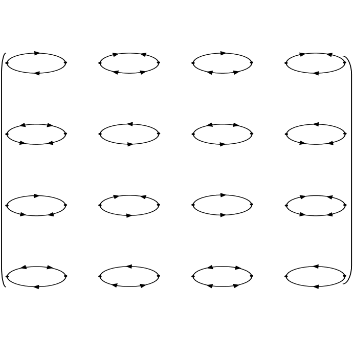
Figure 1: Diagrams corresponding to elements $A^{(-)}_{\pi\nu,ik}$ of the free two-quasiparticle propogator of Eq. (43). Upper (lower) lines correspond to propagation of proton (neutron) quasiparticles.

The expression for the elements of the free two-quasiparticle propagator (43) can be obtained making use of the regular and anomalous single-particle Green’s functions for Fermi-systems with nucleon pairing in analogue way as it was done in monograph [[21]] to describe the Fermi-system response to a single-particle probing operator acting in the neutral channel. Namely, the matrix $A$ can be depicted as a set of the diagrams shown in Fig. 1. To illustrate this statement, let us consider the system of equations for the elements of the transition potential $v_{i}$. The system follows from Eq. (41) and can be schematically represented as $v_{i}=\sum_{k}F_{i}A^{(-)}_{ik}(\omega=\omega_{s})v_{k}\ .$

Using expression (43) for the free two-quasiparticle propagator, one can obtain the system of the inhomogeneous equations of the pn-QRPA to calculate the strength functions (11) with taking the full basis of the single-particle states into consideration for the particle-hole channel. The system has the form similar to that of Eqs. (17), (18) taken in the “symmetric” approximation:

$$\displaystyle S_{J}^{(\mp)}(\omega)=-\frac{1}{\pi}\mathop{\rm Im}\nolimits\sum\limits_{i}\int V_{J}(r)A_{J,1i}^{(\mp)}(r,r^{\prime};\omega)\tilde{V}_{J,i}^{(\mp)}(r^{\prime},\omega)\,drdr^{\prime},$$ (44)

$$\displaystyle\tilde{V}_{J,i}^{(\mp)}(r,\omega)=V_{J}(r)\delta_{i1}+\frac{1}{4\pi r^{2}}\sum\limits_{k}\int F^{J}_{i}(rr_{1})A_{J,ik}^{(\mp)}(r_{1},r_{2};\omega)\tilde{V}_{J,k}^{(\mp)}(r_{2},\omega)\,dr_{1}dr_{2}.$$ (45)

The same as in case without pairing, the residues $(r^{(\mp)}_{J})_{s}$ in poles of the strength functions (see Eq. (20)) coincide with the particle-hole strengths of the pn-QRPA excitations corresponding to the probing operators $\hat{V}^{(\mp)}_{J\mu}$.

3.4 Strength functions in single-open-shell nuclei.

We restrict the further consideration to the case of the single-open-shell nuclei. For this case the system of equations (45) for the radial effective operators $\tilde{V}^{(\mp)}_{J,i}(r,\omega)$ is noticeably simplified. Let us consider for definiteness the excitations in the $\beta^{-}$-channel for a nucleus in which only the proton pairing is realized ($\Delta_{n}=0$). Then, according to Eq. (43), the elements $A^{(-)}_{J,12},A^{(-)}_{J,13},A^{(-)}_{J,24},A^{(-)}_{J,34}$ of the free two-quasiparticle propagator equal to zero and the system (45) is reduced to the system of equations only for 2 radial effective operators $\tilde{V}^{(-)}_{J,1}$ and $\tilde{V}^{(-)}_{J,4}$. The elements $A^{(-)}_{J,11},A^{(-)}_{J,14},A^{(-)}_{J,44}$ entering this system can be rewritten in the form which allows one to take the full basis of the single-particle states in the particle-hole channel for both subsystems. To get this form one should put $E_{\pi}=|\varepsilon_{\pi}-\mu_{\pi}|$ for $E_{\pi}>k\Delta_{p}$ ($k\gg 1$) and use the spectral expansion for the radial single-particle Green’s functions in Eq. (43). As a result, we come to the following representation for $A^{(-)}_{J,11}$:

$$\displaystyle A^{(-)}_{J,11}(r_{1},r_{2};\omega)=\sum\limits_{\nu(\pi)}\left(t^{(J)}_{(\pi)(\nu)}\right)^{2}n_{\nu}\chi_{\nu}(r_{1})\chi_{\nu}(r_{2})g_{(\pi)}(r_{1},r_{2};\varepsilon_{\nu}+\omega)+$$ (46)

$$\displaystyle\sum\limits_{(\nu)\pi}\left(t^{(J)}_{(\pi)(\nu)}\right)^{2}v^{2}_{\pi}\chi_{\pi}(r_{1})\chi_{\pi}(r_{2})g_{(\nu)}(r_{1},r_{2};\mu_{\pi}-E_{\pi}-\omega)+$$

$$\displaystyle\mathop{{\sum}^{\prime}}\limits_{\nu\pi}\left(t^{(J)}_{(\pi)(\nu)}\right)^{2}n_{\nu}\chi_{\nu}(r_{1})\chi_{\nu}(r_{2})\chi_{\pi}(r_{1})\chi_{\pi}(r_{2})\times$$

$$\displaystyle\left\{\frac{u^{2}_{\pi}}{\omega-\mu_{p}-E_{\pi}+\varepsilon_{\nu}}+\frac{v^{2}_{\pi}}{\omega-\mu_{p}+E_{\pi}+\varepsilon_{\nu}}-\frac{1}{\omega-\varepsilon_{\pi}+\varepsilon_{\nu}}\right\},$$

where $\mathop{{\sum}^{\prime}}_{\nu\pi}$ denotes the sum, which is taken over the proton states with $E_{\pi}<k\Delta_{p}$ only. For the consistency of the consideration, the same truncation should be used in realization of the BCS model according to the second of Eqs. (31). The corresponding expressions for the elements $A^{(-)}_{J,14}$ and $A^{(-)}_{J,44}$ are:

$$\displaystyle A^{(-)}_{J,14}(r_{1},r_{2};\omega)=-\mathop{{\sum}^{\prime}}\limits_{(\nu)\pi}\left(t^{(J)}_{(\pi)(\nu)}\right)^{2}u_{\pi}v_{\pi}\chi_{\pi}(r_{1})\chi_{\pi}(r_{2})g_{(\nu)}(r_{1},r_{2};\mu_{\pi}-E_{\pi}-\omega)+$$ (47)

$$\displaystyle\mathop{{\sum}^{\prime}}\limits_{\nu\pi}\left(t^{(J)}_{(\pi)(\nu)}\right)^{2}n_{\nu}\chi_{\nu}(r_{1})\chi_{\nu}(r_{2})\chi_{\pi}(r_{1})\chi_{\pi}(r_{2})\left\{\frac{1}{\omega-\mu_{p}-E_{\pi}+\varepsilon_{\nu}}-\frac{1}{\omega-\mu_{p}+E_{\pi}+\varepsilon_{\nu}}\right\},$$

$$\displaystyle A^{(-)}_{J,44}(r_{1},r_{2};\omega)=\mathop{{\sum}^{\prime}}\limits_{(\nu)\pi}\left(t^{(J)}_{(\pi)(\nu)}\right)^{2}u_{\pi}^{2}\chi_{\pi}(r_{1})\chi_{\pi}(r_{2})g_{(\nu)}(r_{1},r_{2};\mu_{\pi}-E_{\pi}-\omega)+$$ (48)

$$\displaystyle\mathop{{\sum}^{\prime}}\limits_{\nu\pi}\left(t^{(J)}_{(\pi)(\nu)}\right)^{2}n_{\nu}\chi_{\nu}(r_{1})\chi_{\nu}(r_{2})\chi_{\pi}(r_{1})\chi_{\pi}(r_{2})\left\{\frac{v^{2}_{\pi}}{\omega-\mu_{p}-E_{\pi}+\varepsilon_{\nu}}+\frac{u^{2}_{\pi}}{\omega-\mu_{p}+E_{\pi}+\varepsilon_{\nu}}\right\}.$$

The equations (44)–(48) realize a continuum version of the pn-QRPA (pn-QCRPA) on the truncated basis of the BCS problem in proton-open-shell nuclei.

To go to the case when only the neutron pairing is realized, the equations (46)–(48) should be changed by the substitution $\pi\leftrightarrow\nu,\ p\leftrightarrow n,\ \omega\to-\omega$. As before, the expression for the elements of the free two-quasiparticle propagator $A^{(+)}$ can be obtained from the corresponding elements $A^{(-)}$ by the substitution $\pi\leftrightarrow\nu,\ p\leftrightarrow n$.

4 Calculation results

4.1 Choice of the model parameters

Parametrization of the isoscalar part of the mean field $U_{0}(x)$ along with the values of the parameters used in the calculations have been described in details in [[29]]. The dimensionless intensities $f_{J}$ of the Landau-Migdal forces of Eq. (4) are chosen as usual: $F_{J}=f_{J}\cdot 300$ MeV fm³. The value $f_{0}=f^{\prime}=1.0$ of the parameter $f^{\prime}$ determining the symmetry potential according to Eq. (7) is also taken from the [[29]], where the experimental nucleon separation energies have been satisfactorily described for closed-shell subsystems in a number of nuclei. The value of the dimensionless intensity $f_{1}=g^{\prime}$ of the spin-isovector part of the Landau-Migdal forces $g^{\prime}=0.8$ is chosen to reproduce within the CRPA the experimental energy of the GTR in ²⁰⁸Pb parent nucleus [[17]].

The strength of the monopole particle-particle interaction $G_{0}$ is chosen to reproduce the experimental pairing energies (actually, we identify the pairing energy with $\Delta$, obtained by solving the BCS-model equations (31)). The summation in the second of the equations is limited by the interval of 7 MeV above and below the Fermi level. The same truncation is used in the expressions like (46)–(48) for the elements of the free two-quasiparticle propagator. Comparing the calculated value of the nucleon separation energy $B_{\beta}^{calc}\simeq-\mu_{\beta}+\Delta_{\beta}$ with the corresponding experimental one can be considered as a test of the used version of the BCS model. The parameters of the BCS model along with $B_{\beta}^{calc}$ and $B_{\beta}^{exp}$ are listed in the Table 1. Note also, that the strength of the spin-spin particle-particle interaction $G_{1}$ is chosen equal to $G_{0}$, which seems close to the realistic ones used in literature. Such a choice allows us to simplify the calculation control using the $(EWSR)_{1}$, because the “particle-particle” part of this sum rule goes to zero in accordance with Eq. (38). Another reason for the choice is the “soft” spin-isospin SU(4)-symmetry, which is roughly realized in nuclei (see, e.g., [[26]]).

4.2 F (C) strength functions

The F(C) strength functions have been calculated within the CRPA for the ²⁰⁸Pb parent nucleus according to Eqs. (17), (18) and within the pn-QCRPA for ${}^{90}Zr$ and tin isotopes according to Eqs. (44), (45) or their modifications. The “cut-off” parameter $k=3$ was used in calculations of the radial propagators of Eqs. (46)–(48). All above-mentioned equations have been taken for $J=0$. The following characteristics of the F strength distribution have been deduced from the calculated F strength functions: the IAR energy $E_{IAR}$; the mean energy $\bar{E}_{IVMR}^{(-)}$ of the IVMR^(-); relative Fermi strength $x$ for 3 energy intervals: the vicinity of the IAR, IVMR^(-), and IVMR⁽⁺⁾; relative energy-weighted Fermi strength $y$ for these 3 energy regions. As for the low-energy interval, for all nuclei in question the values of $x$ are below 0.1% (except for ⁹⁰Zr, where $x\simeq$0.2%). The value of $(EWSR)_{0}$ entering the definition of $y$ has been calculated according to Eq. (15) with the nucleon densities modified by the nucleon pairing. All the characteristics of the F strength distribution are listed in the Table 2 along with the experimental IAR energies. To check the selfconsistency of the model, the parameter $z=\left|\frac{\int S^{(-)}_{C}(\omega)\,d\omega}{\int S^{(-)}_{F}(\omega)\omega^{2}\,d\omega}-1\right|$ has also been calculated.

4.3 GT strength functions

The GT strength functions have been calculated within the CRPA for the ²⁰⁸Pb parent nucleus according to Eqs. (17), (18) and within the pn-QCRPA for ⁹⁰Zr and tin isotopes according to Eqs. (44), (45) or their modifications taken for $J=1$. ¿From the calculated GT strength functions the relative GT strength $x$ and relative energy-weighted GT strength $y$ for 4 energy intervals (low-energy, the vicinity of the GTR, high-energy, and the vicinity of the IVSMR⁽⁺⁾) have been deduced. The value of $(EWSR)_{1}^{p\mbox{\it-}h}$ entering the definition of $y$ has been calculated according to Eq. (16) with the nucleon densities and the occupation numbers modified by the nucleon pairing. The value of $(EWSR)_{1}^{p\mbox{\it-}p}$ defined according to Eq. (38) equals zero because of putting $G_{1}=G_{0}$ in our calculations. The values of the parameters $x$ and $y$ are listed in the Table 3 along with the calculated energies of the GTR. The values of the relative strengths $x_{s}=r_{s}/(N-Z)$ of the GT doorway states calculated according to Eq. (20) with and without taking the nucleon pairing into consideration are shown in the Figs. 2–4 (solid and dotted vertical lines, respectively).

The coupling of the GT doorway states with many-quasiparticle configurations is taken into consideration phenomenologically and is described in average over the energy in terms of the smearing parameter $I(\omega)$ simulating the mean spreading width of the doorway states. Following [[17]] we choose $I(E_{x})$ to be an universal function revealing saturation at rather high excitation energies:

$$I(E_{x})=\alpha\frac{E_{x}^{2}}{1+E_{x}^{2}/B^{2}},$$ (49)

where $\alpha$ and $B$ are adjustable parameters, $E_{x}$ is the excitation energy in the daughter nucleus. Equation (49) is close to the parametrization of the intensity of the optical-potential imaginary part obtained within the modern version of an optical model. The choice of the parameters $\alpha=0.09$ MeV^-1 and $B=7$ MeV has allowed us to describe satisfactorily the total widths of a number of the isovector giant resonances (including GTR) in the ²⁰⁸Pb parent nucleus [[19]]. In this work the energy-averaged GT strength function $\bar{S}_{1}^{(-)}$ is calculated as $\bar{S}_{1}^{(-)}(\omega)=S_{1}^{(-)}(\omega+{\rm i}I(E_{x})/2)$ using the same parametrization of $I$, where $S_{1}^{(-)}$ is the GT strength function calculated according to the CRPA or pn-QCRPA equations. The calculation results are shown in the Figs. 2–4 (thin line). The calculated energy dependence in the vicinity of the GTR is approximated by the Breit-Wigner formulae to get both the GTR energy $E_{GTR}$ and width $\bar{\Gamma}_{GTR}$. The values of $E_{GTR}$ obtained thereby and $\bar{\Gamma}_{GTR}$ along with the values calculated without taking the nucleon pairing into consideration (in brackets) are listed in the Table 3 in comparison with the corresponding experimental data.

We analyze the effect of the isospin splitting according to Eqs. (24), (26) without taking the nucleon pairing into consideration because this effect turns out to be weak even for such a rather light parent nucleus as ⁹⁰Zr. In this case there is the only $T_{0}$ component of the GT strength function in ⁹⁰Nb (due to the $g_{9/2}\to g_{7/2}$ M1 transition in the proton subsystem). Its relative strength and energy are $x_{>}=4.7$ % and $E_{>}=12.8$ MeV, respectively. It leads to a decrease in the relative strength and energy of the GTR equal to $x_{>}$ and $x_{>}(E_{>}-E_{<})/x_{<}=0.3$ MeV, respectively, as compared with the values found within the CRPA.

5 Discussion of the results

5.1 Summary concerned to the approach

We have extended the CRPA approach, used previously in [[17]–[19]] for describing the GTR and the IAR in closed-shell nuclei, and have formulated a version of the pn-QCRPA approach for describing the GT and F strength distributions in open-shell nuclei. The common ingredients of both approaches are the following: the phenomenological isoscalar part of the nuclear mean field; the isovector part of the Landau-Migdal particle-hole interaction; the isospin selfconsistency condition being used to calculate the symmetry potential; mean Coulomb field calculated in the Hartree approximation; the use of the full basis of the single-particle states in the particle-hole channel and, as a result, formulating the continuum versions of the RPA; a phenomenological description of the coupling of the particle-hole doorway states with many-quasiparticle configurations in terms of the mean doorway-state spreading width (the smearing parameter).

The specific feature of the developed pn-QCRPA approach is the use of an isospin-invariant particle-particle interaction to describe both the nucleon pairing phenomenon in neutral channels and particle-particle interaction in charge-exchange channels. The method to check the isospin selfconsistency, which could be violated by the use of a truncated basis of single-particle states in particle-particle channel within the approach, is also used.

5.2 F (C) strength distribution

The present results (Table 2) show at the microscopical level that the isospin is a good quantum number for medium-heavy mass nuclei. In particular, the IAR exhausts almost all F strength. The rest is mainly exhausted by the IVMR. The heavier a nucleus is, the more the relative F strength of the IVMR becomes. Similar results have also been obtained for the energy-weighted Fermi-strength distribution.

The appropriate choice of the particle-particle interaction along with the use of the same truncated basis of single-particle states in the neutral and charge-exchange channels ensure the isospin selfconsistency of the approach (the calculated values of $z$ are found to be less than $0.1\%$). For the same reason, the effect of the nucleon pairing on the F strength distribution is small.

The systematic lowing of the IAR energy compared with the experimental value is a shortcoming of the approach, possibly caused by the absence of the full selfconsistency.

5.3 GT strength distribution

For all nuclei in question, the calculated GT strength function splits into three main regions (see Table 3 and Figs. 2–4). The main part of the GT strength (70–80%) is exhausted by the GTR. In the case of ²⁰⁸Bi, the calculated GTR relative strength is found to be in a reasonable agreement with the respective experimental value $x^{exp}_{GTR}=(60\pm 15)\%$ [[4]]. The spin-quadrupole part of the particle-hole interaction is taken into account only for ²⁰⁸Bi. As a result, the calculated GTR relative strength is decreased from 68% to 66% and the low-energy GT strength is noticeably redistributed. In the case of ⁹⁰Nb, the difference between experimental and calculated results is somewhat larger: $x^{exp}_{GTR}=(39\pm 4)\%$ [[6]], $x^{exp}_{GTR}=(61\pm 8)\%$ ($x^{exp}=(66^{+20}_{-10})\%$ up to 20 MeV in excitation energy) [[5]]. This could be partly due to the well-known quenching effect which has been discussed during the last two decades. This effect is not finally established experimentally well enough and its discussion is out of the scope of this work.

The calculated high-energy part of the the GT strength distribution is mainly exhausted by the IVSMR and its satellites. This part is relatively large for ²⁰⁸Bi (about 19%) and decreases up to about 9% for ⁹⁰Nb (4.6% due to the IVSMR and 4.5% due to $T_{>}$ component of the GTR). The low-energy part contains the weakly-collectivized GT states, which can be related to those found in [[11, 13, 14]]. The nucleon pairing leads to noticeable enriching of the calculated low-energy part of the the GT strength distribution in open-shell nuclei. This fact is in a qualitative agreement with respective experimental data (shown in Figs. 2–4). The calculated values $x_{low}/x_{GTR}$ 19.2% and 25.8% are found to agree reasonably with the corresponding experimental values 28.2% and 30.4% [[7]] for ⁹⁰Nb and ²⁰⁸Bi, respectively. Bearing in mind also the above-mentioned calculated and experimental values of $x_{GTR}$, we can expect that the quenching effect is not so noticeable as it is usually assumed.

The configurational splitting of the main GT state is found for some single-open-shell nuclei (Figs. 2, 3). In the case of the ⁹⁰Zr parent nucleus, the splitting is caused by the direct spin-flip transition $1f_{7/2}^{n}\to 1f_{5/2}^{p}$, which becomes possible due to the proton pairing and whose energy is close to the GTR energy calculated without taking this transition into account. The value of the splitting (about 0.5 MeV) is found to be rather small. For this reason, the total GTR width is only slightly increased. In the case of the Sn isotopes, the strongest effect caused by the $1h_{11/2}^{n}\to 1h_{9/2}^{p}$ transition is found for the ¹²⁰Sn parent nucleus. The splitting energy is found to be rather large and leads to a noticeable increase of the total GTR width. The calculated isospin splitting energy for ⁹⁰Nb (4.0 MeV) is found to be in good agreement with the respective experimental one (4.4 MeV [[6]]).

In conclusion, we incorporate the BCS model in the CRPA method to formulate a version of the partially self-consistent pn-QCRPA approach for describing the multipole particle-hole strength distributions in open-shell nuclei. The approach is applied to describe the Fermi and Gamow-Teller strength functions in a wide excitation-energy interval for a number of single- and double-closed-shell nuclei. A reasonable description of available experimental data is obtained.

Authors are grateful to Prof. M. Fujiwara and Prof. A. Faessler for thorough reading the manuscript and many valuable remarks. V.A.R. would like to thank the Graduiertenkolleg “Hadronen in Vakuum, in Kernen und Sternen” (GRK683) for supporting his stay in Tübingen and Prof. A. Faessler for hospitality.

Table 1: Calculated values of the pairing gap $\Delta_{\beta}$ along with the calculated and experimental proton and neutron separation energies $B_{p,n}^{calc,\ exp}$. The monopole pairing strength $G_{0}$ is also given

Nucleus	$G_{0}\cdot A$,	$\Delta_{\beta}$,	$B_{n}^{calc}$,	$B_{p}^{calc}$,	$B_{n}^{exp}$,	$B_{p}^{exp}$,
	MeV	MeV	MeV	MeV	MeV	MeV
90Zr	14.0	1.15	11.5	8.2	11.98	8.36
112Sn	11.5	1.3	10.9	7.5	10.79	7.56
114Sn	11.5	1.4	10.7	8.3	10.30	8.48
116Sn	11.5	1.3	9.9	9.1	9.56	9.28
118Sn	11.5	1.4	9.7	9.9	9.33	10.00
120Sn	11.5	1.4	9.4	10.7	9.11	10.69
122Sn	11.5	1.4	9.1	11.5	8.81	11.4
124Sn	11.5	1.2	8.7	12.3	8.49	12.10

Table 2: Calculated characteristics of the Fermi strength distribution along with respective experimental data [[3, 4, 7]] (see the text for details)

Parent	x, %			y, %			$E_{IAR}$ , MeV		$\bar{E}_{IVMR}$ ,
nucleus	IAR	high	(+)	IAR	high	(+)	calc.	exp.	MeV
90Zr	98.6	1.5	0.5	94.2	4.2	0.9	4.6	5.0	27.1
112Sn	97.8	2.4	0.6	92.9	5.6	0.7	5.6	6.2	25.0
114Sn	98.0	2.4	0.5	93.5	5.5	0.7	6.8	7.3	25.3
116Sn	97.3	2.4	0.4	93.2	5.4	0.5	7.8	8.4	25.5
118Sn	97.7	2.4	0.3	93.9	5.3	0.5	8.8	9.3	26.0
120Sn	97.6	2.4	0.3	93.9	5.2	0.4	9.7	10.2	26.4
122Sn	97.5	2.4	0.2	94.0	5.2	0.3	10.7	11.2	26.8
124Sn	96.8	2.5	0.2	93.4	5.2	0.3	11.7	12.2	27.3
208Pb	94.4	3.1	0.2	89.8	6.2	0.2	14.4	15.1	32.5

Table 3: Calculated characteristics of the Gamow-Teller strength distribution along with respective experimental data [[3, 4, 7]] (see the text for details).

Parent	x, %				y, %				$E_{GTR}$, MeV		$\bar{\Gamma}_{GTR}$, MeV
nucleus	low	GTR	high	${(+)}$	low	GTR	high	${(+)}$	calc.	exp.	calc.	exp.
90Zr	14.8	76.5	9.1	4.1	6.7	79.3	8.2	2.4	8.8 (8.4)	8.8$\pm$0.1	3.1 (2.7)	4.8$\pm$0.2
112Sn	21.5	77.1	7.5	2.1	13.1	72.6	11.8	1.9	9.2 (9.2)	$8.94\pm 0.25$	3.4 (2.8)	$4.8\pm 0.3$
114Sn	20.6	75.6	6.9	3.8	12.4	72.8	11.3	1.6	9.9 (9.5)	$9.39\pm 0.25$	4.4 (2.8)	$5.6\pm 0.3$
116Sn	17.6	74.8	7.1	0.9	10.3	73.0	11.8	1.1	10.7 (10.3)	$10.04\pm 0.25$	5.2 (3.0)	$5.5\pm 0.3$
118Sn	17.1	75.6	7.0	2.0	9.3	74.1	11.6	1.3	11.9 (11.5)	$10.61\pm 0.25$	4.9 (3.3)	$5.7\pm 0.3$
120Sn	28.6	61.4	7.8	1.2	19.5	63.4	12.8	1.3	13.0 (12.5)	$11.45\pm 0.25$	4.5 (3.4)	$6.4\pm 0.3$
122Sn	22.3	65.6	8.5	0.6	14.1	67.4	13.8	0.8	13.8 (13.5)	$12.25\pm 0.25$	3.9 (3.5)	$5.6\pm 0.3$
124Sn	21.6	66.9	9.0	0.6	12.5	68.5	14.3	0.8	14.4 (14.3)	$13.25\pm 0.25$	3.6 (3.5)	$5.2\pm 0.3$
208Pb	17.0	65.8	18.7	0.7	9.1	63.8	25.0	0.7	15.6	15.6$\pm$0.2	3.7	3.54$\pm$0.25

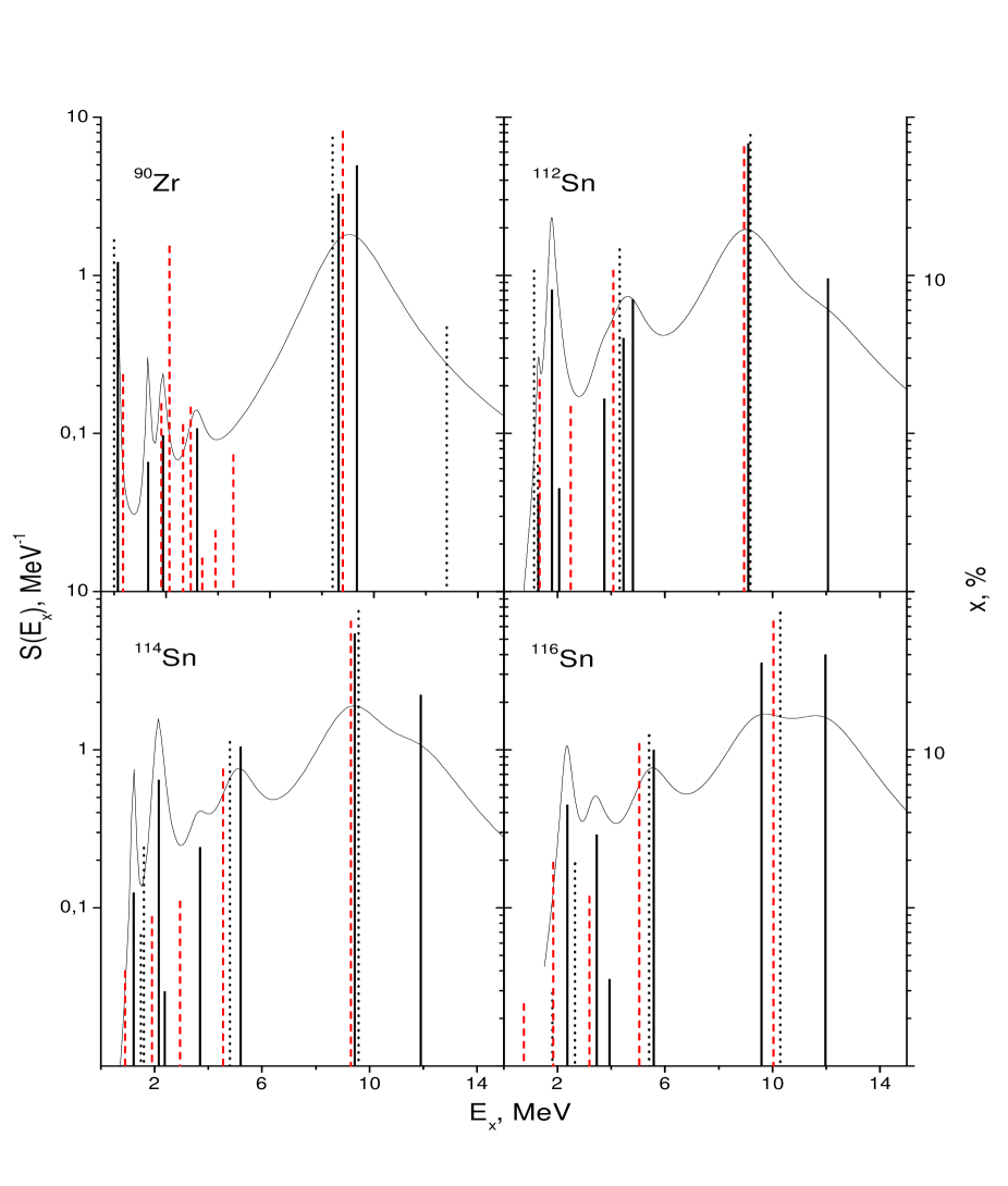
Figure 2: The relative GT strengths $x$ in ⁹⁰Nb, ^112-116Sb calculated within the pn-QCRPA (solid vertical line) and CRPA (dotted vertical lines) in comparison with the respective experimental data [[3, 7]] (dashed vertical lines). The smeared pn-QCRPA GT-strength distribution $\bar{S}$ is also shown (thin solid lines)

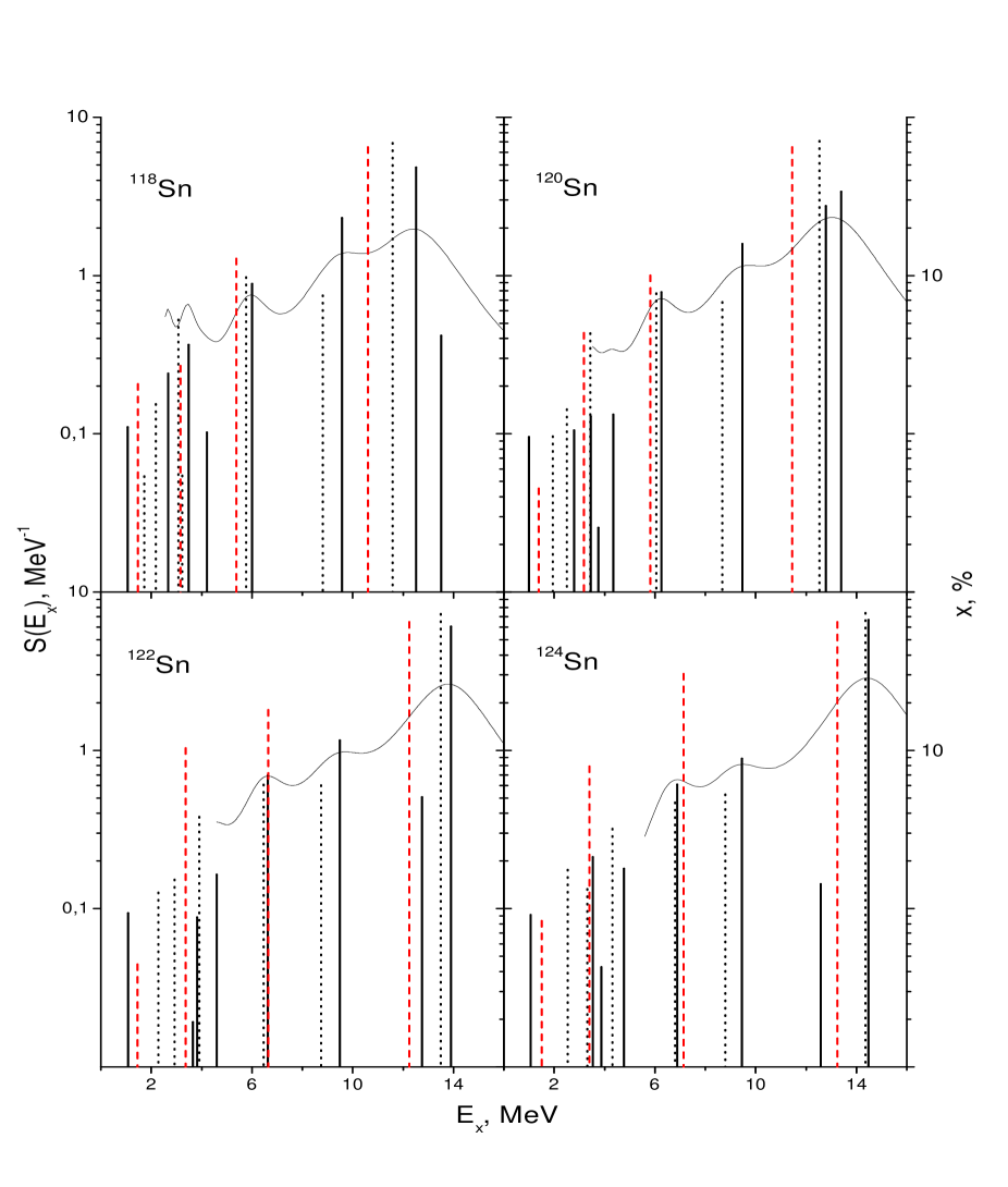
Figure 3: The same as in the Fig. 2 but for the ^118-124Sb (the experimental data are taken from [[3]])

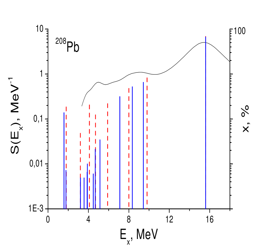
Figure 4: The relative GT strengths $x$ in ²⁰⁸Bi calculated within the CRPA (solid vertical lines) along with the respective smeared distribution $\bar{S}$ (thin solid line). The experimental data are taken from [[7]] (dashed vertical lines)

References

• [1] A. Bohr and B.R. Mottelson, Nuclear structure (New York, Benjamin, 1969), Vol.1.
• [2] J. Suhonen and O. Civitarese, Phys. Rep. 300, 123 (1998).
• [3] J. Jänecke et al., Phys. Rev. C 48, 2828 (1993); K. Pham et al., Phys. Rev. C 51, 526 (1995); M. Fujiwara et al., Nucl. Phys. A 599, 223c (1996).
• [4] H. Akimune et al., Phys. Rev. C 52, 604 (1995).
• [5] M. Moosburger et al., Phys. Rev. C 57, 602 (1998).
• [6] J. Jänecke et al., Nucl. Phys. A 687, 270c (2001).
• [7] A. Krasznahorkay et al., Phys. Rev. C 64, 067302 (2001).
• [8] T. Wakasa et al., Phys. Rev. C 55, 2909 (1997).
• [9] T.Wakasa et al., Nucl. Phys. A 687, 26c (2001).
• [10] N. Auerbach, Phys. Rep. 98, 273 (1983).
• [11] Yu.V. Gaponov and Yu.S. Lyutostanskii, Yad. Fiz. 19, 62 (1974); Fiz. Elem. Chastits At. Yadra 12, 1234 (1981).
• [12] N. Auerbach and A. Klein, Phys. Rev. C 30, 1032 (1984).
• [13] V.G. Guba, M.A. Nikolaev, and M.G. Urin, Phys. Lett. B 218, 283 (1989); Sov. J. Nucl. Phys. 51, 622 (1990).
• [14] H. Sagawa, T. Suzuki, and N. van Giai, Phys. Rev. C 57, 139 (1998); T. Suzuki and H. Sagawa, Eur. Phys. J. A 9, 49 (2000).
• [15] G.F. Bertsch and I. Hamamoto, Phys. Rev. C 26, 1323 (1982);
N.D. Dang, A. Arima, T. Suzuki and S. Yamaji, Phys. Rev. Lett. 79, 1638 (1997);
S. Drożdż, V. Klempt, J. Speth, and J. Wambach, Phys. Lett. B 166, 18 (1986); S. Drożdż, S. Nishizaki, J. Speth, and J. Wambach, Phys. Rep. 197, 1 (1990).
• [16] A. Arima, T. Cheon, K. Shimizu et al., Phys. Lett. B 122, 126 (1983);
T. Suzuki and H. Sakai, Phys. Lett. B455, 25 (1999);
A. Arima, W. Bentz, T. Suzuki, and T. Suzuki, Phys. Lett. B 499, 104 (2001).
• [17] E.A. Moukhai, V.A. Rodin, and M.H. Urin, Phys. Lett. B 447, 8 (1999).
• [18] M.L. Gorelik, and M.H. Urin, Phys. Rev. C 63, 064312 (2001).
• [19] V.A. Rodin and M.H. Urin, Nucl. Phys. A 687, 276c (2001).
• [20] I.N. Borzov, E.L. Trykov, and S.A. Fayans, Sov. J. Nucl. Phys. 52, 627 (1990); I.N. Borzov, S.A. Fayans, and E.L. Trykov, Nucl. Phys. A 584, 335 (1995); I.N. Borzov and S. Goriely, Phys. Rev. C 62, 035501 (2000).
• [21] A.B. Migdal, Theory of finite Fermi-systems and properties of atomic nuclei (Moscow, Nauka, 1983) (in Russian).
• [22] B.L. Birbrair and V.A. Sadovnikova, Sov. J. Nucl. Phys. 20, 347 (1975).
• [23] O.A. Rumyantsev and M.H. Urin, Phys. Lett. B 443, 51 (1998).
• [24] K. Ikeda, S. Fujii and J.I. Fujita, Phys. Lett. 3, 271 (1963).
• [25] M.H. Urin and O.N. Vyazankin, Nucl. Phys. A 537, 534 (1992).
• [26] D.M. Vladimirov, Y.V. Gaponov, Sov. J. Nucl. Phys. 55, 1010 (1992).
• [27] V.A. Rodin and M.H. Urin, Phys. Part. Nucl. 31, 490 (2000).
• [28] V.G. Soloviev, Theory of Complex Nuclei (Pergamon, Oxford, 1976).
• [29] M.L. Gorelik, S. Shlomo, and M.H. Urin, Phys. Rev. C 62, 044301 (2000).