Proton-neutron quadrupole interactions: an effective contribution to the pairing field

Abstract

We point out that the proton-neutron energy contribution, for low multipoles (in particular for the quadrupole component), effectively renormalizes the strength of the pairing interaction acting amongst identical nucleons filling up a single-j or a set of degenerate many-j shells. We carry out the calculation in lowest-order perturbation theory. We perform a study of this correction in various mass regions. These results may have implications for the use of pairing theory in medium-heavy nuclei and for the study of pairing energy corrections to the liquid drop model when studying nuclear masses.

1 Introduction

The pairing force, which expresses in the most succint way the preference of nucleon pairs to become bound into $J^{\pi}=0^{+}$ states in the atomic nucleus, has been widely used in many applications in the study of nuclear structure properties [1, 2, 3, 4]. The special structure of the monopole pairing force has allowed to study the classification of nucleons that occupy a set of single-particle orbitals. The quasi-spin scheme [2, 3], or, closely related the seniority quantum number $v$ [5], leads to single-j and degenerate many-j shell exactly solvable models. They can be used as benchmarks to compare with approximation methods. Moreover, use of monopole pairing forces allows to determine an important energy contribution when evaluating total nuclear binding energies.

Another important characteristic of the nucleon-nucleon effective interaction acting inside atomic nuclei is expressed through the long-range components of this interaction [6]. The low multipoles and the quadrupole component, in particular, are essential in generating low-lying nuclear collective phenomena. They also contribute to the mean-field energy (binding energy in the nuclear ground state, deformation properties,…) of the atomic nucleus.

These two components of the nucleon-nucleon effective force have formed a keystone to understand many facets of nuclear structure: from few valence nucleons near to closed-shell configurations as well as in those situations where many valence protons and neutrons are actively present outside closed shells. They are essential ingredients of any shell-model (or present large-scale shell-model) calculation, even though in most of them either model interactions are constructed explicitely or deduced from more realistic nucleon-nucleon potentials (see refs. [7, 8, 9, 10, 11] to cite just some recent shell-model studies).

It is our aim now, in the study of nuclear masses and two-neutron separation energies $S_{2n}$, to understand better the interplay of global energy contributions (liquid-drop energy as determined from simple models [12, 13] or from more sophisticated microscopic-macroscopic methods [14, 15, 16, 17, 18, 19]) with local correlation effects. The latter contributions arise from specific nuclear structure effects taking pairing and low-multipole force components into account. Local correlation effects can come from various origins such as (i) the presence of closed-shell discontinuities, (ii) the appearance of local zones of nuclear deformation, and (iii) configuration mixing or shape mixing that will show up in the ground state of the nucleus itself. A number of results have been published recently on this topic [20, 21].

In the present paper, we study how monopole pairing (that forms an essential ingredient in all local energy correlations) can accomodate long-range forces and as such give rise to an effective pairing force that can later be used when (i) applying pairing theory in order to study lowest-order broken-pair excitations in medium-heavy nuclei, and (ii) see how, following results obtained recently by Fossion et al. [21] concerning the study of two-neutron separation energies $S_{2n}$, the new pairing corrections on top of the liquid-drop energy could reproduce local binding energy (and $S_{2n}$) variations even better.

In section 2, we succintly indicate the results of monopole pairing in a single-j shell, and we explicitely evaluate the proton-neutron quadrupole-quadrupole contribution to the ground-state energy. Thereby we observe that its effect leads to an effective pairing contribution. In section 3, we discuss applications in various mass regions in order to estimate the effect of this renormalized ’pairing-like’contribution.

In the conclusion, we indicate that this extra effect may well be interesting when studying nuclear structure properties not too far from closed shells in which the interactions amongst identical nucleons dominate the proton-neutron interaction effects.

2 Shell-model correlations

As discussed in the introductory section, the interplay of the monopole pairing force and the proton-neutron low-multipole deformation-driving force components are essential ingredients of any shell model calculation. The aim of the present paper is to point out that, to lowest order, the proton-neutron quadrupole part can be incorporated as a renormalization of the pairing force strength. Of course, this means that applications will stick to regions near to closed shells where the proton-neutron energy contribution is not the dominant part. In open shells, with both valence protons and neutrons active, one has to treat both components (monopole pairing and low-multipole proton-neutron part) on equal footing.

We first give a short reminder of the monopole pairing correlation energy part, considering the nucleons are filling a single-j shell (or a set of degenerate-j shells). Secondly, we study the proton-neutron energy correction (quadrupole interaction) to be superposed to the monopole pairing part.

2.1 Pairing energy corrections

The Hamiltonian, describing the most simple case of a monopole pairing force between $n$ identical valence nucleons interacting in a single-j shell, with a given strength $G$, is described as

$$\hat{H}=-G\sum_{m,m^{\prime}>0}a^{\dagger}_{jm}a^{\dagger}_{j-m}a_{j-m^{\prime}}a_{jm^{\prime}}(-1)^{2j+m+m^{\prime}}.$$ (1)

The ground state of such a system corresponds to a state where the nucleons are coupled in pairs of angular momentum $J=0$. As a consequence the ground state has seniority $\upsilon=0$,

$$|n,\upsilon=0\rangle=(S^{+}_{j})^{n/2}|0\rangle,$$ (2)

where

$$S^{+}_{j}=\frac{1}{\sqrt{\Omega}}\sum_{m>0}(-1)^{j+m}a^{+}_{jm}a^{+}_{j-m}.$$ (3)

The binding energy of this system becomes

$$BE^{\scriptsize\mbox{pairing}}=\frac{G}{4}(2\Omega-n+2)n=G(\Omega-N+1)N,$$ (4)

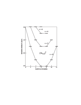
Figure 1: Spectrum for a pure pairing force within the $1h_{11/2}$ orbital, i.e. for the $(1h_{11/2})^{n}$ spectrum, with seniority $\upsilon=0$, $\upsilon=2$, $\upsilon=4$, and $\upsilon=6$ as a function of the particle number $n$. The pairing strength $G$ has been chosen as $G=0.25$ MeV [4].

where $N$ is the number of valence nucleon pairs and $\Omega$ is the shell degeneracy, $\Omega=j+1/2$. In a system with valence protons and neutrons, interacting through monopole pairing forces between alike nucleons, one has to consider the expression (4) for protons and for neutrons separately. As an illustration of this interaction (see figure 1), we shown the spectrum of a monopole pairing force. From expression (4), the two-neutron separation energy can be easily deduced, with as a result

$$S_{2n}^{\scriptsize\mbox{pairing}}=G(\Omega_{\nu}+2-n_{\nu})=G(\Omega_{\nu}+2-2N_{\nu}),$$ (5)

where $n_{\nu}$ is the number of valence neutrons, $N_{\nu}$ the number of valence neutrons pairs and $\Omega_{\nu}=j_{\nu}+1/2$ is the shell degeneracy for neutrons.

2.2 The quadrupole energy contribution

As discussed before, we now evaluate the energy contribution in the ground state that is due to the proton-neutron quadrupole-quadrupole interaction. The quadrupole proton-neutron Hamiltonian can be written as,

$$\hat{H}=\kappa\hat{Q}_{\pi}\cdot\hat{Q}_{\nu},$$ (6)

where $\hat{Q}$ is the quadrupole operator for protons and neutrons, respectively, and $\cdot$ stands for the scalar product. The main characteristic of the quadrupole operator is that it induces the breaking of pairs, promoting pairs coupled to $J^{\pi}=0^{+}$ into pairs coupled to $J^{\pi}=2^{+}$, thereby changing the seniority quantum number $\upsilon$ and causing a core-polarization effect [22]. To a first approximation, the ground state of the system will change from a condensate of proton and neutron pairs coupled to $J^{\pi}=0^{+}$ into a superposition of the state of expression (2) together with a new one where one-proton and one-neutron pairs coupled to $J^{\pi}=2^{+}$ are induced,

$$|N_{\pi}\otimes N_{\nu}\rangle=|S_{j\pi}^{N_{\pi}}\otimes S_{j\nu}^{N_{\nu}};J=0\rangle+\xi|S_{j\pi}^{N_{\pi}-1}D_{j\pi}\otimes S_{j\nu}^{N_{\nu}-1}D_{j\nu};J=0\rangle,$$ (7)

where the operator

$$D^{+}_{j}=\sum_{m>0}(-1)^{j-m}\langle jmj-m|20\rangle a^{\dagger}_{jm}a^{\dagger}_{j-m},$$ (8)

will create a pair of nucleons coupled to $J=2$.

Taking into account that the quadrupole energy contribution is small with respect to the monopole pairing interaction energy, the most straightforward way in order to fully determine the state vector in expression (7) is to use perturbation theory. The mixing coefficient results as

$$\xi={\kappa\alpha\over\Delta E_{\alpha}},$$ (9)

where we use the shorthand notation

$$\alpha=\langle S_{j\pi}^{N_{\pi}}\otimes S_{j\nu}^{N_{\nu}};J=0|\hat{Q}_{\pi}\cdot\hat{Q}_{\nu}|S_{j\pi}^{N_{\pi}-1}D_{j\pi}\otimes S_{j\nu}^{N_{\nu}-1}D_{j\nu};J=0\rangle,$$ (10)

and define the energy difference

$$\Delta E_{\alpha}=-E_{2^{+}_{\pi}}-E_{2^{+}_{\nu}},$$ (11)

in which $E_{2^{+}_{\rho}}$ ($\rho=\pi,\nu$) denotes the excitation energies of states with one $J=2$ proton or neutron pair, respectively.

The energy correction due to the quadrupole force is then given by evaluating the matrix element of the Hamiltonian (6) using the state vector (7). For a system where the forces are monopole pairing and quadrupole proton-neutron interactions only, this results into the binding energy expression

$$BE=BE^{\scriptsize\mbox{pairing}}+2{\kappa^{2}\alpha^{2}\over(-\Delta E_{\alpha})},$$ (12)

where $BE^{\scriptsize\mbox{pairing}}$ corresponds to the result given in expression (4).

Due to the schematic structure of the states appearing in expression (10), it is now possible to obtain an explicit expression for this matrix element [5]. In a first step, we decouple the proton and neutron parts with the result

$$\alpha = \frac{1}{\sqrt{5}}\langle(S_{j\pi})^{N_{\pi}};J=0\|\hat{Q}_{\pi}\|(S_{j\pi})^{N_{\pi}-1}D_{j\pi};J=2\rangle$$ (13)

$$\times \langle(S_{j\nu})^{N_{\nu}};J=0\|\hat{Q}_{\nu}\|(S_{j\nu})^{N_{\nu}-1}D_{j\nu};J=2\rangle.$$

Using the appropriate reduction formulae one arrives to the result

$$\alpha=\frac{1}{\sqrt{5}}\sqrt{N_{\pi}(\Omega_{\pi}-N_{\pi})}\sqrt{N_{\nu}(\Omega_{\nu}-N_{\nu})}\frac{\langle\hat{Q}_{\pi}\rangle\langle\hat{Q}_{\nu}\rangle}{\sqrt{(\Omega_{\pi}-1)(\Omega_{\nu}-1)}},$$ (14)

where,

$$\langle\hat{Q}_{\pi}\rangle=\langle S_{j\pi}\|\hat{Q}_{\pi}\|D_{j\pi}\rangle=\frac{2}{\sqrt{2j_{\pi}+1}}\langle j_{\pi}\|\hat{Q}_{\pi}\|j_{\pi}\rangle,$$ (15)

and

$$\langle\hat{Q}_{\nu}\rangle=\langle S_{j\nu}\|\hat{Q}_{\nu}\|D_{j\nu}\rangle=\frac{2}{\sqrt{2j_{\pi}+1}}\langle j_{\pi}\|\hat{Q}_{\nu}\|j_{\pi}\rangle.$$ (16)

The expressions (15) and (16) can be even more simplified if one uses harmonic oscillator wave functions and uses the expression for the quadrupole operator,

$$\hat{Q}=\sum_{i}r_{i}^{2}Y_{2}(\theta_{i},\varphi_{i}),$$ (17)

resulting into

$$\langle\hat{Q}_{\rho}\rangle = \frac{2}{\sqrt{2j_{\rho}+1}}(N_{ho}+\frac{3}{2})\langle j_{\rho}\|Y_{2}(\theta,\varphi)\|j_{\rho}\rangle$$ (18)

$$= \sqrt{\frac{5}{\pi}}(N_{ho}+\frac{3}{2})\frac{\frac{3}{4}-j_{\rho}(j_{\rho}+1)}{\sqrt{(2j_{\rho}-1)j_{\rho}(j_{\rho}+1)(2j_{\rho}+3)}}.$$

Here $\rho=(\pi,\nu)$, $Y_{2}(\theta,\varphi)$ denotes the spherical harmonic with $L=2$ and $N_{ho}$ describes the number of quanta of the shell.

One finally obtains a closed expression for the binding energy,

$$BE=BE^{\scriptsize\mbox{pairing}}+\frac{2}{5}\frac{\kappa^{2}}{(-\Delta E_{\alpha})}\frac{N_{\pi}(\Omega_{\pi}-N_{\pi})N_{\nu}(\Omega_{\nu}-N_{\nu})}{(\Omega_{\nu}-1)(\Omega_{\pi}-1)}\langle Q_{\pi}\rangle^{2}\langle Q_{\nu}\rangle^{2}.$$ (19)

If we are interested in the study of binding energies within a set of isotopes (thus $\Omega_{\pi}$ and $N_{\pi}$ are fixed numbers), and by defining the coefficient $\overline{C}$ as follows,

$$\overline{C}=\frac{2}{5}\frac{\kappa^{2}}{(-\Delta E_{\alpha})}\frac{N_{\pi}(\Omega_{\pi}-N_{\pi})}{(\Omega_{\nu}-1)(\Omega_{\pi}-1)}\langle\hat{Q}_{\pi}\rangle^{2}\langle\hat{Q}_{\nu}\rangle^{2},$$ (20)

one obtains a “correlated” binding energy expression in the ground state

$$BE^{\scriptsize\mbox{correlated}}=BE^{\scriptsize\mbox{pairing}}+\overline{C}(\Omega_{\nu}-N_{\nu}+1)N_{\nu}-\overline{C}N_{\nu}.$$ (21)

We can incorporate the proton-neutron quadrupole binding energy contribution as a renormalisation of the pairing strength in regions near closed shells where pairing dominates the proton-neutron quadrupole interaction. In these regions and for medium-heavy nuclei, which can be characterized by single-particle orbitals with large degeneracies $\Omega_{\nu}$ (see also discussion in sect. 3 and tables 1 and 3), the energy contribution for the third term in eq. (21) is much smaller than the energy contribution for the second term at the beginning of the shell (small $N_{\nu}$) and up towards midshell ($N_{\nu}\approx\Omega_{\nu}/2$). The total “correlated” binding energy then becomes to a good approximation,

$$BE^{\scriptsize\mbox{correlated}}\approx(G+\overline{C})(\Omega_{\nu}-N_{\nu}+1)N_{\nu}.$$ (22)

So, one obtains a form, identical to the original monopole pairing energy expression, albeit with a new coupling strength. This equation can be applied to the region where detailed values for binding energies in the $Z\sim 40$ and $Z\sim 50$ nuclei (see table 3) are known.

In the next section we shall evaluate, in some detail, the range of values for the coefficients $G$ and $\overline{C}$ in medium-heavy nuclei. These results will show how good our idea is in reality, that proton-neutron quadrupole-quadrupole forces can be used to define an effective pairing force between identical nucleons.

An interesting result is that in evaluating the two-neutron separation energy, the quadratic part drops out and one obtains a strictly linear behavior in $N_{\nu}$ with the result

$$S_{2n}^{\scriptsize\mbox{quadrupole}}(N_{\nu})=(G+\overline{C})(\Omega_{\nu}+2-2N_{\nu})-\overline{C}.$$ (23)

This is essentially the same result as was obtained using a pure monopole pairing force (see expression (5)) except for the small correction factor $\overline{C}$ (which we still have to prove).

The former discussion which uses first order perturbation theory to determine the wave function (eq. (7)) can be repeated for pure hexadecupole or higher multipole interaction Hamiltonians (using eq. (6), replacing $\hat{Q}_{\rho}$ by the appropriate multipole operator). Each higher multipole separately will give a smaller energy contribution to the binding energy, so that only a limited number of multipoles will be important. Using higher order perturbation theory to determine the modified wave functions, extra energy contributions become are possible that come from different multipoles acting together. These higher order contributions result in a different $N_{\nu}$ dependence than the contributions from separately treated multipoles. These higher order effects will be of minor importance. In the present paper, we do not aim at carrying out a detailed shell model study - in that case the multipole Hamiltonian should rather be diagonalised - but we find it quite surprising that the lowest-order effect induced by proton-neutron residual forces comes about as a ’renormalization’ of the original monopole pairing force. We find this an interesting observation.

3 The pairing and quadrupole strength: some specific applications and how well works the above approximation

In the present section, we make a detailed study of the correction factor $\overline{C}$ , mainly concentrating on medium-heavy nuclei. We compare this effective pairing force with the monopole pairing strength that is derived from standard parametrizations, in this mass region.

• The monopole pairing strength $G$.

  An average value of $G$ for medium-mass and heavy nuclei is $25/A$ MeV [23]. However, this value can significantly change in different mass regions, ranging from $G=19/A$ MeV, for the regions $Z\sim 40-50$, to $G=30/A$ MeV for Pb nuclei [24].

  As an example, for ₅₂Te isotopes ($A\approx 106-152$) the pairing strength is $G\approx 0.15$ MeV, and for ₄₂Mo isotopes ($A\approx 84-128$) $G\approx 0.18$ MeV.

• The effective pairing strength $\overline{C}$, obtained from the proton-neutron quadrupole force.

  In order to estimate the value of $\overline{C}$, using the method discussed in section 2, we have to reduce the set of more realistic single-particle orbitals that are not degenerate and are typical for a given mass region, into a large, degenerate single-j shell. In table 1, we indicate those values of $j$ as well as the degeneracies for different major shells or subshells in the regions $Z\sim 40$ and $Z\sim 50$. As example of isotopes with $Z\sim 40$ we consider the ₄₈Cd (N${}_{\pi}=1$), ₄₂Mo (N${}_{\pi}=1$), ₄₄Ru (N${}_{\pi}=2$), and ₄₆Pd (N${}_{\pi}=2$) nuclei . For the region with $Z\sim 50$, we consider the ₅₂Te (N${}_{\pi}=1$), ₅₄Xe (N${}_{\pi}=2$), ₅₆Ba (N${}_{\pi}=3$), and ₅₈Ce (N${}_{\pi}=4$) nuclei. For both shells we take as number of quanta N${}_{ho}=4$, which covers a shell from $40$ to $70$ nucleons and is in agreement with table 1.

  Another ingredient necessary in order to determine $\overline{C}$ (see expression (20)) is the value of $\Delta E_{\alpha}=-E_{2^{+}_{\pi}}-E_{2^{+}_{\nu}}$ which can be estimated from experimental energy systematics of the first $2^{+}$ excitation energy [4]. This results for the $Z\sim 50$ region into a maximum value of $\Delta E_{\alpha}\simeq-2$ MeV [25] and for the $Z\sim 40$ region, a slightly higher value $\Delta E_{\alpha}\simeq-2.5$ MeV is obtained [22].

  The final element in order to calculate $\overline{C}$ is the strength of the proton-neutron interaction $\kappa$. There exist realistic values of the quadrupole strength in the context of the IBM [26, 27], $\kappa_{0}$, that can be easily related with the value of $\kappa$ appearing in expressions (6) and (20) through the following relation [22]:

  $$\kappa=\frac{5\kappa_{0}\sqrt{\Omega_{\pi}\Omega_{\nu}}}{\sqrt{\frac{2}{\Omega_{\pi}-1}}\sqrt{\frac{2}{\Omega_{\nu}-1}}\langle j_{\pi}\|\hat{Q}_{\pi}\|j_{\pi}\rangle\langle j_{\nu}\|\hat{Q}_{\nu}\|j_{\pi}\rangle}.$$ (24)

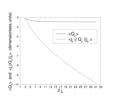
Figure 2: Plot of the values for $\left<Q_{\rho}\right>$ and $\left<j_{\rho}\left\|Q_{\rho}\right\|j_{\rho}\right>$ for $j_{\rho}$ going from $3/2$ to $31/2.$ As one can see, $\left<Q_{\rho}\right>$ is nearly a constant for changing $j_{\rho}$.

  As can be verified from table 2 and noted in figure 2, the reduced matrix elements $|\langle j_{\rho}\|Q_{\rho}\|j_{\rho}\rangle|$ increase linearly with $j_{\rho}$, but this variation is almost completely compensated through the presence in the numerator of the factors $\Omega_{\rho}$. This then results in values for $\kappa$ that are almost independent of the value of $j_{\rho}$ ($\Omega_{\rho}$). On the other hand, the values of $\langle\hat{Q}_{\rho}\rangle$ and $\langle\hat{Q}_{\rho}\rangle^{2}$ (the third factor in expression (20)) do not change dramatically with $j_{\rho}$ in the range $j_{\rho}=\frac{3}{2}-\frac{31}{2}$. This is an important outcome which implies that the value of $\overline{C}$ is not strongly dependent on the particular $j$ ($\Omega$) value of the proton and/or neutron orbitals (degeneracies) that the nucleons are occupying (state independence). This results into robust values of $\overline{C}$.

  Having discussed the various elements that are necessary in order to derive a schematic, albeit rather realistic, estimate of $\overline{C}$, we present, in table 3, the values for different nuclei in the regions $Z\sim 40$ and $Z\sim 50$. We point out that two alternatives shell closures have been used.

  Inspecting the results, as given in table 3, it becomes clear that the effective pairing correction, stemming from the proton-neutron interaction, can be at maximal of the order of 10-15% of the regular monopole pairing strength. The precise values depend somewhat on the degeneracies of the proton and neutron shell-model spaces that are used in order to describe the various series of isotopes.

As a conclusion, on notices that the quadrupole constant $\overline{C}$ is smaller than the monopole pairing constant $G$ by a factor varying in between 5 to 25. Therefore, quadrupole and low-multipole force components give rise to contributions to the binding energy that exhibit the same structure (except for some smaller corrections) as those resulting from monopole pairing forces solely. The particular number dependence of the binding energy (see expression (22)) occurs through the common factor $(\Omega-N+1)N$ with $\Omega$ the degenarcy of the shell that is filling up with identical nucleons.

4 Conclusion

In the present paper, we have shown that pure monopole pairing can accomodate long-range forces (we have studied in particular the case of proton-neutron quadrupole forces but the extension to other low multipoles is now straightforward) using perturbation theory, and as such give rise to an effective pairing force. This latter effect renormalizes the monopole pairing energy with an amount that can vary between 5 to 25%.

This result came partly as a surprise and did come up when we were studying the variation of nuclear binding energies and, more in particular, two-neutron separation energies $S_{2n}$ over a large region of nuclei (rare-earth mass region, nuclei in the neutron-deficient Pb region [20, 21]). In the above papers, we have studied the local correlation energy within the framework of the Interacting Boson Model (IBM) [26, 27, 28] and outlined a prescription in order to derive nuclear masses within a single framework.

Recently, we have started the study of nuclear binding energies and two-neutron separation energies $S_{2n}$ in medium-heavy nuclei (mass A=100-130 region) using the same concepts but also trying to evaluate the local correlation energy taking into account the shell-model structure and the residual interactions (pairing, quadrupole proton-neutron interactions) [29]. In order to study these local energy corrections that appear on top of the global energy (liquid drop energy, macroscopic-microscopic energy studies - see refs. given in the introduction), we have studied in the present paper the modifications that proton-neutron forces induce on the strict monopole pairing energy. We have shown that the dependence on nucleon number (e.g. neutron number when studying series of isotopes) for the effective pairing contribution is identical to the nucleon number dependence of the monopole pairing force. In going through a series of isotopes, changing the number of neutron pairs, $N_{\nu}$, the effective pairing force will likewise exhibit a neutron number dependence through the presence of the factor $\overline{C}$ (see expression 20).

Therefore, we aim at (i) applying pairing theory to study lowest-order broken-pair excitations in medium-heavy nuclei, and (ii) see how, following up on results obtained recently by Fossion et al. [21] concerning the study of two-neutron separation energies $S_{2n}$, the effective pairing corrections on top of the liquid-drop energy could reproduce local binding energy (and $S_{2n}$) variations even better.

5 Acknowledgements

The authors are grateful to discussions with G. Bollen, S. Schwarz and A. Kohl on very precise mass measurements and their importance for testing nuclear structure studies that have lead to the present investigations. They are grateful to the referee for a number of constructive remarks in order to improve on both form and content. They thank the “FWO-Vlaanderen”, NATO for a research grant CRG96-098 and the IWT for financial support during this work. One of the authors (KH) is most grateful for the hospitality at ISOLDE/CERN and the support in finishing the present investigation.

Table Captions

Table 1: Degeneracies and associated single-j shell configurations for regions $Z\sim 40$ and $Z\sim 50$.

$Z\sim 40$
Shell	Degeneracy	$j$
$Z=40-50$	$\Omega_{\pi}=5$	$j_{\pi}=9/2$
$N=50-64$	$\Omega_{\nu}=7$	$j_{\nu}=13/2$
$N=50-82$	$\Omega_{\nu}=16$	$j_{\nu}=31/2$
$Z\sim 50$
Shell	Degeneracy	$j$
$Z=50-82$	$\Omega_{\pi}=16$	$j_{\pi}=31/2$
$Z=50-64$	$\Omega_{\pi}=7$	$j_{\pi}=13/2$
$N=50-82$	$\Omega_{\nu}=16$	$j_{\nu}=31/2$

Table 2: Values for $\left<Q_{\rho}\right>,\left<Q_{\rho}\right>^{2}$ and $\left<j_{\rho}\left\|Q_{\rho}\right\|j_{\rho}\right>$ (see expressions 15, 16 and 18) for $j_{\rho}$ going from $3/2$ to $31/2.$

$j_{\rho}$	$\left<Q_{\rho}\right>$	$\left<Q_{\rho}\right>^{2}$	$\left<j_{\rho}\|Q_{\rho}\|j_{\rho}\right>$
3/2	-3.10	9.62	-3.10
5/2	-3.31	11.00	-4.06
7/2	-3.38	11.46	-4.78
9/2	-3.41	11.67	-5.40
11/2	-3.43	11.78	-5.94
13/2	-3.44	11.85	-6.44
15/2	-3.44	11.89	-6.89
17/2	-3.45	11.92	-7.32
19/2	-3.45	11.94	-7.72
21/2	-3.45	11.96	-8.11
23/2	-3.46	11.97	-8.47
25/2	-3.46	11.98	-8.82
27/2	-3.46	11.99	-9.48
31/2	-3.46	12.00	-9.79

Table 3: Values of $\overline{C}$ ( in MeV) for different nuclei and different mass regions.

$Z\sim 40$
Shells	Mo	Cd	Ru	Pd
$\Omega_{\pi}=5$, $\Omega_{\nu}=16$	0.0062	0.0062	0.0093	0.0093
$\Omega_{\pi}=5$, $\Omega_{\nu}=7$	0.0059	0.0059	0.0079	0.0079
$Z\sim 50$
Shells	Te	Xe	Ba	Ce
$\Omega_{\pi}=16$, $\Omega_{\nu}=16$	0.0091	0.017	0.0240	0.029
$\Omega_{\pi}=7\phantom{1}$, $\Omega_{\nu}=16$	0.0036	0.006	0.0073	0.0073

Figure Captions

References

- [1] P.J. Brussaard and P.W.M. Glaudemans, Shell-model applications in nuclear spectroscopy (North-Holland, Amsterdam, 1977).
- [2] P. Ring and P. Schuck, The nuclear many-body problem (Springer-Verlag, New York, Heidelberg, Berlin, 1980).
- [3] I. Talmi, Simple models of complex nuclei (Harwood Academic Publishers, 1993).
- [4] K. Heyde, The nuclear shell-model (Springer-Verlag, Berlin, Heidelberg, New York, 1994).
- [5] A. de Shalit and I. Talmi, Nuclear shell theory (Academic Press, New York and London, 1963).
- [6] A.Bohr and B.Mottelson, Nuclear Structure, vol.2 (Benjamin, New-York, 1975).
- [7] E.K.Warburton, J.A.Becker and B.A.Brown, Phys.Rev.C 41, 1147 (1990).
- [8] A.Poves and J.Retamosa, Nucl.Phys.A571, 221 (1994).
- [9] E.Caurier, F.Nowacki, A.Poves and J.Retamosa, Phys.Rev.C 58, 2033 (1998).
- [10] T.Otsuka, T.Mizusaki, Y.Utsuno and M.Honma,ENAM98, Exotic Nuclei and Atomic Masses, eds. B.M.Sherill, D.J.Morrissey and C.N.Davids, 1998,Am.Inst.of Physics
- [11] D.J.Dean, M.T.Ressell, M.Hjorth-Jensen, S.E.Koonin, K.Langanke and A.P.Zuker, Phys.Rev.C 59, 2474 (1999).
- [12] A.H. Wapstra, Handbuch der Physik Vol. 1, (1958).
- [13] A.H. Wapstra and N.B. Gove, Nucl. Data Tables 9,267 (1971).
- [14] P. Möller and J.R. Nix, Nucl. Phys. A 361,117 (1981).
- [15] P. Möller and J.R. Nix, At. Data Nucl. Data Tables 39, 213 (1988).
- [16] P. Möller, J.R. Nix, W.D. Myers, and W.J. Swiatecki, At. Data Nucl. Data Tables 59, 185 (1995).
- [17] Y. Aboussir, J.M. Pearson, A.K. Dutta, and F. Tondeur, At. Data Nucl. Data Tables 61,127 (1995).
- [18] G.A. Lalazissis, S. Raman, and P. Ring, At. Data Nucl. Data Tables 71,1 (1999).
- [19] S. Goriely, F. Tondeur, and J.M. Pearson, At. Data Nucl. Data Tables 77, 311 (2001).
- [20] S.Schwarz, F.Ames, G.Audi, D.Beck, G.Bollen, C.De Coster, J.Dilling, R.Fossion, J.E.Garcia-Ramos, F.Herfurth, K.Heyde, J.-J.Kluge, A.Kohl, D.Lunney, R.B.Moore, H.Raimbault-Hartmann, J.Szerypo and the ISOLDE collaboration,Nucl. Phys. A693 , 533 (2001).
- [21] R.Fossion, C.De Coster, J.E.Garcia-Ramos, T.Werner and K.Heyde, Nucl. Phys. A (2001), in print
- [22] K.Heyde, J.Jolie, J.Moreau, J.Ryckebusch, M.Waroquier, P.Van Duppen, M.Huyse and J.L.Wood, Nucl.Phys.A446, 189 (1987).
- [23] D.Rowe, Nuclear Collective Motion, (Methuen, London, 1970)
- [24] L.S. Kisslinger and R.A. Sorensen, Mat. Fys. Medd. Dan. Vid. Selsk. 32, n∘ 9 (1960).
- [25] K.Heyde and J.Sau, Phys.Rev.C 33, 1050 (1986).
- [26] F.Iachello and A.Arima, The Interacting Boson Model, (Cambridge University Press,1987)
- [27] A.Frank and P.Van Isacker, Algebraic Methods in Molecular and Nuclear Structure Physics, (Wiley, New-York,1994)
- [28] R. F. Casten and D. D. Warner, Rev. Mod. Phys. 60, 389 (1988).
- [29] J. E. Garcia-Ramos,R. Fossion, C. De Coster and K. Heyde, work in progress