Non–Local Potentials and Rotational Bands of Resonances in Ion Collisions

Abstract

Sequences of rotational resonances (rotational bands) and corresponding antiresonances are observed in ion collisions. In this paper we propose a description which combines collective and single–particle features of cluster collisions. It is shown how rotational bands emerge in many–body dynamics, when the degeneracies proper of the harmonic oscillator spectra are removed by adding interactions depending on the angular momentum. These interactions can be properly introduced in connection with the exchange–forces and the antisymmetrization, and give rise to a class of non–local potentials whose spectral properties are analyzed in detail. In particular, we give a classification of the singularities of the resolvent, which are associated with bound states and resonances. The latter are then studied using an appropriate type of collective coordinates, and a hydrodynamical model of the trapping, responsible for the resonances, is then proposed. Accordingly, we derive, from the uncertainty principle, a spin–width of the unstable states which can be related to their angular lifetime.

1 Introduction

The phase–shifts $\delta_{\ell}$ in the $\alpha$–nucleus elastic scattering have, at low energy, the following behaviour: first, they rise passing through $\pi/2$, and cause a sharp maximum in the energy dependence of $\sin^{2}\delta_{\ell}$ that corresponds to a resonance; then they decrease, crossing $\pi/2$ downward, and produce what is called an echo or an antiresonance [1, 2]. Typical examples are the phase–shifts in the $\alpha$–$\alpha$ or in $\alpha$–⁴⁰Ca elastic scattering (see refs. [3, 4, 5]). A second relevant feature is that the resonances and, correspondingly, the antiresonances, are organized in an ordered sequence and produce a rotational band of levels whose energy spectrum can be fitted by an expression of the form $E_{\ell}=A+B\,\ell(\ell+1)$, where $\ell$ is the (approximate) orbital angular momentum of the level, and $A$ and $B$ are constants almost independent of $\ell$. Finally, the widths of the resonances increase as a function of the energy; consequently, at higher energy, the rotational resonances evolve into surface waves that can be explained as due to the diffraction by the target, which is regarded as an opaque (or partially opaque) obstacle. These features, which emerge in a particularly clear form in the $\alpha$–nucleus scattering are however characteristic of a very large class of heavy ion collisions, like e.g., ¹²C–¹²C, ¹²C–¹⁶O, ²⁴Mg–²⁴Mg, ²⁸Si–²⁸Si, etc. (see [6] and the references quoted therein).

Though rotational resonances can be described, with some approximation, within the framework of the two–body problem, antiresonances necessarily involve the many–body properties of the interaction. In fact, the rotational levels can be regarded as produced by the trapping of the incoming projectile which rotates, for a certain time, around the target; thus, we have the energy spectrum of a rigid rotator. Conversely, the two–body model is totally inadequate for explaining the echoes. In this case, the two interacting particles (e.g., $\alpha$ particles or ⁴⁰Ca ions) cannot simply be treated as bosons, because the wavefunction of the whole system must be antisymmetric with respect to the exchange of all the nucleons, including those belonging to different clusters. Then, the fermionic character of the nucleons emerges, and from the antisymmetrization a repulsive force derives; accordingly, the phase shifts $\delta_{\ell}$ decrease, and antiresonances are produced. We are thus led to combine the collective and the single–particle features of cluster collisions.

In section 2 the many–body problem, treated by means of the Jacobi coordinates, will be briefly sketched. By introducing potentials of harmonic oscillator type, it can be observed the formation of clusters whose ground–state wavefunction can be represented by the product of gaussians. Furthermore, if the degeneracies, proper of the harmonic oscillator, are removed by introducing interactions which depend on the angular momentum, then rotational bands emerge from the many–body dynamics.

In section 3 the relationship between the Jacobi coordinates and the relative coordinates of the interacting clusters is addressed. We are thus led to consider the wavefunction which describes the relative motion of the clusters. In particular, the antisymmetrization and the exchange character of the nuclear forces yield non–local potentials. To this end, it is worth remembering that the derivation of non–local potentials from many–body dynamics has been extensively studied in the past [7]. The procedures commonly used are: the resonating group method [8], the complex generator coordinate technique [9], and the cluster coordinate method [10]. Their common goal is to provide a microscopic description of the nuclear processes that, starting from a nucleon–nucleon potential and employing totally antisymmetric wavefunctions, can evaluate bound states and scattering cross sections from an unified viewpoint. All these methods have been remarkably successful at a computational level, and they will not be considered hereafter since our main interest here concerns the spectral analysis associated with non–local potentials. The mathematical tool used in this connection is the Fredholm alternative [11], which allows us to study the analytical properties of the resolvent associated with the integro–differential equation of the relative motion, and the main properties of bound states, resonances and antiresonances generated by an appropriate class of non–local potentials. Particular attention is devoted to the fact that the non–local potentials represent angular–momentum dependent interactions and, therefore, in view of the results obtained in section 2, they can appropriately describe rotational bands.

Section 4 is devoted to the rotational resonances regarded as a collective phenomenon. To this end, we introduce a type of collective coordinates (called $Z$–coordinates) and first analyze the relationship between Jacobi and $Z$–coordinates, and then between the latter and the relative coordinates of the interacting clusters. Then, in this scheme, we can introduce a hydrodynamical model of the trapping which is able to generate the resonances. Finally, from this model and through the uncertainty principle, a spin–width, which is proper of rotational resonances, will be defined.

In this paper we focus on the following questions which we think have not received enough attention so far:

• An algebraic–geometric analysis which shows how rotational bands emerge from the many–body dynamics (see section 2).

• The spectral analysis associated with non-local potentials that can give a classification of the resolvent singularities corresponding to bound states and resonances (see section 3).

• The relationship between Jacobi and $Z$–coordinates, which allows us to describe the collective features of the resonances, and to introduce the spin–width proper of the resonances (see section 4).

2 An Outline of the Algebraic–Geometric Approach to Rotational Bands

For the reader’s convenience, in this section we briefly review the Jacobi and the hyperspherical coordinates (very well known in the literature [12, 13, 14]), focusing on those algebraic–geometric aspects which play a relevant role in the following.

First, let us consider the case of three particles of equal mass $m$, whose positions are described by the vectors ${\bf r}_{k}=(x_{k},y_{k},z_{k})$, $(k=1,2,3)$. The kinetic energy operator reads

$$T=-\frac{1}{2m}\left(\Delta_{1}+\Delta_{2}+\Delta_{3}\right),~{}~{}~{}~{}~{}(\hbar=1)\,,$$ (1)

where $\Delta_{k}:\equiv\partial^{2}/\partial x_{k}^{2}+\partial^{2}/\partial y_{k}^{2}+\partial^{2}/\partial z_{k}^{2}$, $(k=1,2,3)$. We can now introduce the Jacobi and center of mass coordinates, which are defined as follows:

$$\displaystyle\mbox{\boldmath$\xi$}_{1} = \frac{{\bf r}_{1}-{\bf r}_{2}}{\sqrt{2}},$$ (2)

$$\displaystyle\mbox{\boldmath$\xi$}_{2} = \left(\frac{2}{3}\right)^{1/2}\left(\frac{{\bf r}_{1}+{\bf r}_{2}}{2}-{\bf r}_{3}\right),$$ (3)

$$\displaystyle{\bf R}_{\mbox{\tiny C.M.}} = \frac{{\bf r}_{1}+{\bf r}_{2}+{\bf r}_{3}}{3}~{},~{}~{}~{}~{}~{}|{\bf r}_{k}|=\sqrt{x_{k}^{2}+y_{k}^{2}+z_{k}^{2}}\,.$$ (4)

The kinetic energy operator can be written in terms of these coordinates as

$$T=-\frac{1}{2m}\left\{\Delta_{{\mbox{\boldmath$\scriptstyle\xi$}}_{1}}+\Delta_{{\mbox{\boldmath$\scriptstyle\xi$}}_{2}}+\frac{1}{3}\Delta_{{{\bf R}}_{\mbox{\tiny C.M.}}}\right\},$$ (5)

where

$$\Delta_{{\mbox{\boldmath$\scriptstyle\xi$}}_{i}}\equiv\frac{\partial^{2}}{[\partial(\mbox{\boldmath$\xi$}_{i})_{x}]^{2}}+\frac{\partial^{2}}{[\partial(\mbox{\boldmath$\xi$}_{i})_{y}]^{2}}+\frac{\partial^{2}}{[\partial(\mbox{\boldmath$\xi$}_{i})_{z}]^{2}},~{}~{}(i=1,2),~{}~{}~{}$$ (6)

$$\Delta_{{{\bf R}}_{\mbox{\tiny C.M.}}}\equiv\frac{\partial^{2}}{[\partial({\bf R}_{\mbox{\tiny C.M.}})_{x}]^{2}}+\frac{\partial^{2}}{[\partial({\bf R}_{\mbox{\tiny C.M.}})_{y}]^{2}}+\frac{\partial^{2}}{[\partial({\bf R}_{\mbox{\tiny C.M.}})_{z}]^{2}},~{}~{}$$ (7)

$(\mbox{\boldmath$\xi$}_{i})_{x},(\mbox{\boldmath$\xi$}_{i})_{y},(\mbox{\boldmath$\xi$}_{i})_{z}$ and $({\bf R}_{\mbox{\tiny C.M.}})_{x},({\bf R}_{\mbox{\tiny C.M.}})_{y},({\bf R}_{\mbox{\tiny C.M.}})_{z}$ denoting the $x,y,z$ components of the vectors $\mbox{\boldmath$\xi$}_{i}$ and ${\bf R}_{\mbox{\tiny C.M.}}$, respectively. Then, the kinetic energy of the center of mass can be separated from that of the relative motion $T_{R}$:

$$T_{R}=-\frac{1}{2m}\left\{\Delta_{\mbox{\boldmath$\scriptstyle\xi$}_{1}}+\Delta_{\mbox{\boldmath$\scriptstyle\xi$}_{2}}\right\}.$$ (8)

Now, it is convenient to combine the vectors $\mbox{\boldmath$\xi$}_{1}$ and $\mbox{\boldmath$\xi$}_{2}$ into a single vector ${{\bf\Xi}}={\mbox{\boldmath$\scriptstyle\xi$}_{1}\choose\mbox{\boldmath$\scriptstyle\xi$}_{2}}$, whose Cartesian components will be denoted by ${\bf\Xi}_{1},{\bf\Xi}_{2},\ldots,{\bf\Xi}_{6}$. Thus, we can consider a sphere embedded in ${\mathord{\mathbb{R}}}^{6}$ whose radius is $\rho^{2}=\xi_{1}^{2}+\xi_{2}^{2}$, and, accordingly, represent the components of ${\bf\Xi}$ in terms of the spherical coordinates $(\rho,\theta_{1},\ldots,\theta_{5})$ as follows:

$$\Xi_{1} = \rho\sin\theta_{5}\sin\theta_{4}\cdots\sin\theta_{1},$$

$$\Xi_{2} = \rho\sin\theta_{5}\sin\theta_{4}\cdots\cos\theta_{1},$$

$$\cdots \cdots\cdots$$ (9)

$$\Xi_{5} = \rho\sin\theta_{5}\cos\theta_{4},$$

$$\Xi_{6} = \rho\cos\theta_{5}.$$

In terms of spherical coordinates the Laplace–Beltrami operator $\Delta$ reads [15]

$$\Delta = \frac{1}{\rho^{5}}\frac{\partial}{\partial\rho}\left(\rho^{5}\frac{\partial}{\partial\rho}\right)+\frac{1}{\rho^{2}\sin^{4}\theta_{5}}\frac{\partial}{\partial\theta_{5}}\left(\sin^{4}\theta_{5}\frac{\partial}{\partial\theta_{5}}\right)+\frac{1}{\rho^{2}\sin^{2}\theta_{5}\sin^{3}\theta_{4}}\frac{\partial}{\partial\theta_{4}}\left(\sin^{3}\theta_{4}\frac{\partial}{\partial\theta_{4}}\right)+\cdots$$ (10)

$$+ \frac{1}{\rho^{2}\sin^{2}\theta_{5}\sin^{2}\theta_{4}\cdots\sin^{2}\theta_{2}}\frac{\partial^{2}}{\partial\theta_{1}^{2}},$$

and, by separating the radial part from the angular one, we get:

$$\Delta=\frac{1}{\rho^{5}}\frac{\partial}{\partial\rho}\left(\rho^{5}\frac{\partial}{\partial\rho}\right)+\frac{1}{\rho^{2}}\Delta_{0},$$ (11)

where $\Delta_{0}$ is the Laplace–Beltrami operator acting on the unit sphere ${\cal S}^{5}$ embedded in ${\mathord{\mathbb{R}}}^{6}$ [15].
Let us introduce the harmonic polynomials of degree $j$ [15], which may be written as $\rho^{j}\Theta_{j}(\theta_{1},\ldots\theta_{5})$. Then, from (11) we get:

$$\Delta\left[\rho^{j}\Theta_{j}(\theta_{1},\ldots\theta_{5})\right]=j(j+4)\rho^{(j-2)}\Theta_{j}(\theta_{1},\ldots\theta_{5})+\rho^{(j-2)}\Delta_{0}\Theta_{j}(\theta_{1},\ldots\theta_{5})=0,$$ (12)

which gives

$$\Delta_{0}\Theta_{j}(\theta_{1},\ldots\theta_{5})=-j(j+4)\Theta_{j}(\theta_{1},\ldots\theta_{5}).$$ (13)

Next, we introduce the momenta associated with the Jacobi coordinates, i.e.,

$$\displaystyle{\bf p}_{\xi_{1}}=\frac{{\bf q}_{1}-{\bf q}_{2}}{\sqrt{2}},$$ (14)

$$\displaystyle{\bf p}_{\xi_{2}}=\left(\frac{2}{3}\right)^{1/2}\left(\frac{{\bf q}_{1}+{\bf q}_{2}}{2}-{\bf q}_{3}\right),$$ (15)

where $({\bf q}_{k})_{x}=m\dot{x}_{k},\,({\bf q}_{k})_{y}=m\dot{y}_{k},\,({\bf q}_{k})_{z}=m\dot{z}_{k}$ $(k=1,2,3)$, and also combine the momenta in a single vector ${\bf P}={{\bf p}_{\xi_{1}}\choose{\bf p}_{\xi_{2}}}$. Then, we consider a potential of the form

$$V(\rho)={\rm G}\left\{|{\bf r}_{1}-{\bf r}_{2}|^{2}+|{\bf r}_{1}-{\bf r}_{3}|^{2}+|{\bf r}_{2}-{\bf r}_{3}|^{2}\right\}=3{\rm G}\rho^{2}.$$ (16)

Again, by separating in the wavefunction $\psi(\rho;\theta_{1},\ldots,\theta_{5})$ the radial variable from the angular ones, we have the following equations:

$$\displaystyle\frac{1}{\rho^{5}}\frac{d}{d\rho}\left(\rho^{5}\frac{dR_{j}}{d\rho}\right)-\frac{j(j+4)}{\rho^{2}}R_{j}+2m\left[E-V(\rho)\right]R_{j}=0,$$ (17)

$$\displaystyle\Delta_{0}\Theta_{j}(\theta_{1},\ldots\theta_{5})=-j(j+4)\Theta_{j}(\theta_{1},\ldots\theta_{5}),$$ (18)

where $E$ denotes the energy. It is easy to see that the solutions of eq. (17) are given by

$$R_{j}(\rho)=\rho^{j}\exp\left[-\frac{1}{2}\sigma^{2}\rho^{2}\right],~{}~{}~{}~{}~{}\sigma=\left(mK\right)^{1/4},$$ (19)

$$\displaystyle E_{j}=(j+3)\,\omega,~{}~{}~{}~{}~{}\omega=\left(\frac{K}{m}\right)^{1/2},$$ (20)

where $K=6{\rm G}$.

It is well known that the group of the permutations of three objects has two one–dimensional representations and one two–dimensional representation. A remarkable fact is that the elements of the permutation group lead to rotations in ${\mathord{\mathbb{R}}}^{6}$, but, as stated in [12], not all the elements of the Lie algebra associated with the $SO(6)$ group treat the three particles equivalently. On the other hand, the sphere ${\cal S}^{5}$ may be regarded as the unit sphere embedded in ${\mathord{\mathbb{C}}}^{3}$ because the complex vector space ${\mathord{\mathbb{C}}}^{3}$ can be identified with the space ${\mathord{\mathbb{R}}}^{6}$. Therefore ${\cal S}^{5}$ may be identified with $SU(3)/SU(2)$, $SU(3)$ acting transitively on ${\cal S}^{5}$. Thus, we are naturally led to introduce the complex vectors:

$$\mbox{\boldmath${\cal Z}$}=\mbox{\boldmath$\xi$}_{1}+i\mbox{\boldmath$\xi$}_{2}, \mbox{\boldmath${\cal Z}$}^{*}=\mbox{\boldmath$\xi$}_{1}-i\mbox{\boldmath$\xi$}_{2},$$ (21)

$${\bf\Pi}={\bf p}_{\xi_{1}}+i{\bf p}_{\xi_{2}}, {\bf\Pi}^{*}={\bf p}_{\xi_{1}}-i{\bf p}_{\xi_{2}},$$ (22)

and to reformulate the problem in the $SU(3)$ group framework. It is easy to see [13] that the operators of interchange of particles turn ${\cal Z}$ into $\mbox{\boldmath${\cal Z}$}^{*}$, and vice–versa, with multiplication by a complex number. Then, we have:

$$\mbox{\boldmath${\cal Z}$}\cdot\mbox{\boldmath${\cal Z}$}^{*}=\xi_{1}^{2}+\xi_{2}^{2}=\rho^{2},$$ (23)

$${\bf\Pi}\cdot{\bf\Pi}^{*}=p_{\xi_{1}}^{2}+p_{\xi_{2}}^{2}=-\Delta.$$ (24)

Next, if we set $m=\hbar=1$, ${\rm G}=1/6$, $(K=1)$, the total Hamiltonian can be written in the following form:

$$H=-\frac{1}{2}\Delta+V=\frac{1}{2}\left({\bf\Pi}\cdot{\bf\Pi}^{*}+\mbox{\boldmath${\cal Z}$}\cdot\mbox{\boldmath${\cal Z}$}^{*}\right).$$ (25)

Now, in order to deal with the harmonic oscillator problem in the Fock space, we introduce the vector creation and annihilation operators [12]:

$${\bf A}^{\dagger}=\frac{1}{\sqrt{2}}\left(\mbox{\boldmath$\xi$}_{1}-i{\bf p}_{\xi_{1}}\right),~{}~{}~{}{\bf A}=\frac{1}{\sqrt{2}}\left(\mbox{\boldmath$\xi$}_{1}+i{\bf p}_{\xi_{1}}\right),$$ (26)

$${\bf B}^{\dagger}=\frac{1}{\sqrt{2}}\left(\mbox{\boldmath$\xi$}_{2}-i{\bf p}_{\xi_{2}}\right),~{}~{}~{}{\bf B}=\frac{1}{\sqrt{2}}\left(\mbox{\boldmath$\xi$}_{2}+i{\bf p}_{\xi_{2}}\right),$$ (27)

which satisfy the following commutation rules

$$\left[A_{k},A^{\dagger}_{p}\right]=\delta_{kp},~{}~{}~{}~{}~{}~{}(k,p=1,2,3),$$ (28)

$$\left[B_{k},B^{\dagger}_{p}\right]=\delta_{kp}.$$ (29)

Finally, in view of the commutation rules (28, 29), the Hamiltonian can be rewritten as follows:

$$H={\bf A}^{\dagger}\cdot{\bf A}+{\bf B}^{\dagger}\cdot{\bf B}+3=N_{A}+N_{B}+3,$$ (30)

where $N_{A}$ and $N_{B}$ are the occupation numbers associated with the operators ${\bf A}^{\dagger}\cdot{\bf A}$ and ${\bf B}^{\dagger}\cdot{\bf B}$, respectively. Then, for the ground state ${|0\!\!>}$, which is characterized by the conditions ${\bf A}{|0\!\!>}={\bf B}{|0\!\!>}=0$, we have $H{|0\!\!>}=3{|0\!\!>}$, which represents the zero point energy; correspondingly, the wavefunction is given by: $\exp[-\rho^{2}/2]$.

Let $j_{1}$ and $j_{2}$ denote the eigenvalues of $N_{A}$ and $N_{B}$, respectively. Then, from (20) and (30), we get: $j=j_{1}+j_{2}$. As is well known, from the Cartan analysis for the $SU(3)$ group, any irreducible representation of $SU(3)$ is completely characterized by two indexes which, in our case, are precisely $j_{1}$ and $j_{2}$ (for the Cartan classification indexes see refs. [12, 16, 17]). In order to investigate how rotational sequences emerge from the three–body dynamics, first the total angular momentum ${\bf L}$ about the center of mass must be introduced, i.e.,

$${\bf L}={\bf r}_{1}\times{\bf q}_{1}+{\bf r}_{2}\times{\bf q}_{2}+{\bf r}_{3}\times{\bf q}_{3}-{\bf R}_{C.M.}\times{\bf p}_{R_{C.M.}},$$ (31)

(where ${\bf p}_{R_{C.M.}}=({\bf q}_{1}+{\bf q}_{2}+{\bf q}_{3})/3)$, which may also be interpreted as the total angular momentum in the center–of–momentum frame, since in this case ${\bf p}_{R_{C.M.}}=0$. Then we have to answer to the following question:

Problem: Determine the $\ell$–values, $\ell(\ell+1)$ being the eigenvalues of ${\bf L}^{2}$, contained in the representation $(j_{1},j_{2})$, where $j_{1}$ and $j_{2}$ are the Cartan indexes of $SU(3)$.

This problem may be rephrased as follows: determine what irreducible representations of the group $SO(3)$, which are labelled by $\ell$, occur in an irreducible representation of the group $SU(3)$. Following Weyl [17], the irreducible representations of the group $U(n)$ are labelled by a set of non–negative integers $f_{1},f_{2},\ldots,f_{n}$ such that: $f_{1}\geq f_{2}\geq\cdots\geq f_{n}$. Next, in the reduction of $U(n)$ to $SU(n)$ the irreducible representations $(f_{1},f_{2},\ldots,f_{n})$ of $U(n)$ remain irreducible under $SU(n)$, but a simplification occurs since certain representations which are not equivalent under $U(n)$ become equivalent under $SU(n)$. Precisely, $(f_{1},f_{2},\ldots,f_{n})$ become equivalent to $(f_{1}-f_{n},\ldots,f_{n-1}-f_{n})$. Consequently, for $SU(3)$, the partition $(f_{1},f_{2},f_{3})$ can be replaced by the differences $k_{1}=f_{1}-f_{3},k_{2}=f_{2}-f_{3}$, which can be related to $j_{1}$ and $j_{2}$ as follows [18]:

$$k_{1}=j_{1}+j_{2}\,,~{}~{}~{}~{}~{}~{}k_{2}=j_{1}.$$ (32)

Furthermore, the Weyl approach gives the expression of the characters, and in particular the dimension, of the irreducible representations of the $U(n)$ or $SU(n)$ group. The formula for the dimension reads [17]

$$\mbox{dim}\,(f_{1},f_{2},\ldots,f_{n})=\prod_{1\leq i<k\leq n}\left(\frac{f_{i}-f_{k}+k-i}{k-i}\right).$$ (33)

Therefore, we answer the question posed by the problem formulated above by means of the following equality:

$$\prod_{1\leq i<k\leq 3}\left(\frac{f_{i}-f_{k}+k-i}{k-i}\right)=\sum_{\ell}\mu_{\ell}(2\ell+1),$$ (34)

where $(2\ell+1)$ is the dimension of the representation $D_{\ell}$ of the rotation group, while $\mu_{\ell}$ denotes the multiplicity, i.e., it gives the number of times the representation $D_{\ell}$ occurs in a certain representation of $SU(3)$. Formula (34) has been obtained by equating the characters of the representation in the specific case of the unit element.

For convenience, we shall continue to use: $j_{1}=k_{2}=f_{2}-f_{3}$ and $j_{2}=k_{1}-k_{2}=f_{1}-f_{2}$. Then, in our case, formula (34) reads

$$(j_{1}+1)(j_{2}+1)\left(\frac{j_{1}+j_{2}+2}{2}\right)=\sum_{\ell}\mu_{\ell}(2\ell+1).$$ (35)

Since the l.h.s of (35) is symmetric in $j_{1}$ and $j_{2}$, it follows that $\mbox{dim}\,(j_{1},j_{2})=\mbox{dim}\,(j_{2},j_{1})$. Now, we consider two cases:

• Let $j_{1}=2n$ ($n$ integer) and $j_{2}=0$; then:

  $$\mbox{dim}\,(j_{1},j_{2})=\mbox{dim}\,(2n,0)=(n+1)(2n+1)=\mbox{dim}\,(D_{0}+D_{2}+\cdots+D_{2n}).$$ (36)

  This means that the $\ell$–values that occur in the representation $(2n,0)$ are: $\ell=0,2,4,\ldots,2n$; $(\mu_{\ell}=1)$. We have thus obtained a rotational band of even parity.

• Let $j_{1}=2n+1$ ($n$ integer) and $j_{2}=0$; then:

  $$\mbox{dim}\,(j_{1},j_{2})=\mbox{dim}\,(2n+1,0)=(n+1)(2n+1)=\mbox{dim}\,(D_{1}+D_{3}+\cdots+D_{2n+1}).$$ (37)

  This means that the $\ell$–values occuring in the representation $(2n+1,0)$ are: $\ell=1,3,5,\ldots,2n+1$; $(\mu_{\ell}=1)$. We have thus obtained a rotational band of odd parity.

Remark 1

The physics of the harmonic oscillator from the group theoretical viewpoint has been thoroughly investigated particularly by Moshinsky and his school (see, in this respect, the excellent book by Moshinsky and Smirnov [19] and the references quoted therein). In particular, the rule that emerges from formula (34) is known in nuclear physics as the Elliott rule [20], and it has been extensively used in connection with nuclear models and, specifically, in the analysis of rotational and shell models [21]; however, as far as we know, it has never been derived and used in the Jacobi approach to the many–body problem.

Let us observe that levels with different values of $\ell$, but with the same value of $j=j_{1}+j_{2}$, are degenerate. In order to remove this degeneracy, other interactions must be added to the harmonic oscillator Hamiltonian. If a term proportional to ${\bf L}\cdot{\bf L}$ is added, we shall have a splitting within the $SU(3)$ multiplets, which is proportional to the square of the total angular momentum ${\bf L}$. Since an energy spectrum proportional to ${\bf L}^{2}$ is just a rotational spectrum, we see that each $SU(3)$ multiplet gives rise to a rotational band. The analysis indicates that rotational bands emerge from the three–body dynamics if angular momentum dependent interactions are acting.

It is straightforward to generalize the Jacobi coordinates to $N$ identical particles of mass $m$. We have:

$$\mbox{\boldmath$\xi$}_{1} = \frac{1}{\sqrt{2}}\left({\bf r}_{1}-{\bf r}_{2}\right),$$

$$\cdots \cdots\cdots$$ (38)

$$\mbox{\boldmath$\xi$}_{N-1} = \frac{1}{\{N(N-1)\}^{1/2}}\left(\sum_{n=1}^{N-1}{\bf r}_{n}-(N-1){\bf r}_{N}\right).$$

Then, we may introduce the hypersphere with radius $\rho$ given by

$$\rho^{2}=\frac{1}{2N}\sum_{k,p=1}^{N}|{\bf r}_{k}-{\bf r}_{p}|^{2}=\mbox{\boldmath$\xi$}_{1}^{2}+\mbox{\boldmath$\xi$}_{2}^{2}+\cdots+\mbox{\boldmath$\xi$}_{N-1}^{2}.$$ (39)

The kinetic energy operator for the $N$–body problem is

$$T=-\frac{1}{2m}\left(\Delta_{1}+\Delta_{2}+\cdots+\Delta_{N}\right),~{}~{}~{}~{}~{}(\hbar=1),$$ (40)

where $\Delta_{k}=\partial^{2}/\partial x_{k}^{2}+\partial^{2}/\partial y_{k}^{2}+\partial^{2}/\partial z_{k}^{2}$, $(k=1,2,\ldots,N)$. Through the Jacobi coordinates, the center of mass kinetic energy can be separated from the kinetic energy of the relative motion $T_{R}$, which reads

$$T_{R}=-\frac{1}{2m}\left(\Delta_{\mbox{\boldmath$\scriptstyle\xi$}_{1}}+\Delta_{\mbox{\boldmath$\scriptstyle\xi$}_{2}}+\cdots+\Delta_{\mbox{\boldmath$\scriptstyle\xi$}_{N-1}}\right),$$ (41)

where $\Delta_{\mbox{\boldmath$\scriptstyle\xi$}_{i}}=\partial^{2}/(\partial(\mbox{\boldmath$\xi$}_{i})_{x})^{2}+\partial^{2}/(\partial(\mbox{\boldmath$\xi$}_{i})_{y})^{2}+\partial^{2}/(\partial(\mbox{\boldmath$\xi$}_{i})_{z})^{2}$, $(i=1,2,\ldots,N-1)$. If we introduce the hyperspherical coordinates $(\rho,\theta_{1},\theta_{2},\ldots,\theta_{3N-4})$, and consider a harmonic oscillator potential of the form:

$$V(\rho)=\frac{1}{2}K\rho^{2},$$ (42)

we can write the Schödinger equation as follows:

$$H\psi=\left(-\frac{1}{2m}\Delta+V\right)\psi\,,$$ (43)

where $\Delta$ is the Laplace–Beltrami operator on the hypersphere of radius $\rho$. By separating the radial variable from the angular ones, we are led to the following expression for the radial part of the wavefunction:

$$R_{j}(\rho)=\rho^{j}\exp\,\left(-\frac{1}{2}\sigma^{2}\rho^{2}\right),$$ (44)

where $\sigma^{2}=m\omega$ $(\omega=\sqrt{K/m})$. Therefore, the radial part of the ground state wavefunction reads

$$R(\rho)=\exp\left(-\frac{m\omega}{2}\rho^{2}\right)=\exp\left(-\frac{m\omega}{2}\sum_{i=1}^{N-1}\xi_{i}^{2}\right).$$ (45)

We can conclude that for any cluster of identical particles the radial wavefunctions of the ground state can be brought to a product of gaussians of the form (45), if the potential has the harmonic oscillator form (42). Finally, we can regard the constant $K$ as a degree of compactness of the cluster, by noting that the peak of the bell–shaped curve representing the function $\exp(-m\omega\rho^{2}/2)$ becomes sharper for increasing values of $K$.

3 Non–Local Potentials and the Associated Spectral Analysis

From the analysis of the previous section we deduce that:

• In order to obtain rotational bands, forces that depend on the angular momentum must be added to the harmonic oscillator potential. In this case a spectrum proportional to ${\bf L}^{2}$ is produced.

• Harmonic oscillator potentials can produce clusters of particles, whose compactness is related to the force constant $K$, and whose radial wavefunctions are expressed as a product of gaussians.

On the other hand the phenomenology shows that rotational bands of resonances emerge from the collisions of clusters. Therefore, in view of point (a), we could try to ascertain if and how these sequences of rotational resonances emerge when interactions, which depend on the angular momentum, are added to harmonic oscillator type forces. In this section we only consider the one–channel case: the elastic channel in the scattering theory.

First, we introduce suitable coordinates for describing cluster collisions. Let ${\bf R}_{i}$ $(i=1,2)$ be the center of mass coordinates of the two clusters. Then assuming, for the sake of simplicity, that the two clusters have the same number $n$ of nucleons, we have:

$${\bf R}_{1} = \frac{{\bf r}_{1}+{\bf r}_{2}+\cdots+{\bf r}_{n}}{n},$$ (46)

$${\bf R}_{2} = \frac{{\bf r}_{n+1}+{\bf r}_{n+2}+\cdots+{\bf r}_{2n}}{n},$$ (47)

where ${\bf r}_{j}$ is the space coordinate of the $j$–th particle, and $2n=N$. The center of mass and the relative coordinates of the two clusters are respectively given by:

$${\bf R}_{\mbox{\tiny C.M.}} = \frac{1}{2}({\bf R}_{1}+{\bf R}_{2}),$$ (48)

$${\bf R} = {\bf R}_{1}-{\bf R}_{2}\,.$$ (49)

Next, we introduce the following internal cluster coordinates ${\bf r}_{j}^{({\rm i})}$ [10]:

$${\bf r}_{j}^{({\rm i})} = {\bf r}_{j}-{\bf R}_{1}\,,~{}~{}~{}\mbox{if}~{}~{}j=1,2,\ldots,n,$$ (50)

$${\bf r}_{j}^{({\rm i})} = {\bf r}_{j}-{\bf R}_{2}\,,~{}~{}~{}\mbox{if}~{}~{}j=(n+1),(n+2),\ldots,2n.~{}~{}~{}~{}~{}$$ (51)

It can easily be verified that the following equality holds true:

$$\rho^{2}=\sum_{j=1}^{n-1}\xi_{j}^{2}=\sum_{j=1}^{n}\left(r_{j}^{({\rm i})}\right)^{2}.$$ (52)

Therefore, for each cluster, the spatial part of the ground state wavefunction can be rewritten in terms of internal cluster coordinates as follows (see (45)):

$$\Phi^{0}_{\mbox{\tiny space}}(1)=\exp\left(-\frac{m\omega}{2}\sum_{j=1}^{n}\left(r_{j}^{({\rm i})}\right)^{2}\right),$$ (53)

$$\Phi^{0}_{\mbox{\tiny space}}(2)=\exp\left(-\frac{m\omega}{2}\sum_{j=n+1}^{2n}\left(r_{j}^{({\rm i})}\right)^{2}\right).$$ (54)

The wavefunction that describes the system composed of the interacting clusters must be antisymmetric with respect to the exchange of all the nucleons, including those belonging to different clusters. Then the wavefunction of the system composed by the two clusters is [10]

$$\Psi= {\cal A} \left\{\left[\Phi^{0}_{\mbox{\tiny space}}(1)\prod_{j=1}^{n}\Phi_{\mbox{\tiny spin}}^{j}(s_{j})\Phi_{\mbox{\tiny isospin}}^{j}(t_{j})\right]\right.$$ (55)

$$\times \left.\left[\Phi^{0}_{\mbox{\tiny space}}(2)\prod_{j=n+1}^{2n}\Phi_{\mbox{\tiny spin}}^{j}(s_{j})\Phi_{\mbox{\tiny isospin}}^{j}(t_{j})\right]\,\chi_{\bf R}^{0}({\bf R})\,\chi_{\mbox{\tiny C.M.}}^{0}({\bf R}_{\mbox{\tiny C.M.}})\right\},$$

where ${\cal A}$ indicates antisymmetrization and normalization, the functions $\Phi_{\mbox{\tiny spin}}^{j}(s_{j})$ and $\Phi_{\mbox{\tiny isospin}}^{j}(t_{j})$ refer respectively to the spin $s_{j}$ and to the isospin $t_{j}$ of the nucleons which compose the clusters, and, finally, $\chi_{\bf R}^{0}({\bf R})$ and $\chi_{\mbox{\tiny C.M.}}^{0}({\bf R}_{\mbox{\tiny C.M.}})$ describe respectively the relative motion of the clusters and the motion of their center of mass. Then, we use the following identity [10]:

$$\sum_{j=1}^{2n}r_{j}^{2}=\sum_{j=1}^{n}\left(r_{j}^{({\rm i})}\right)^{2}+\sum_{j=n+1}^{2n}\left(r_{j}^{({\rm i})}\right)^{2}+\frac{n}{2}\left\{({\bf R}_{1}-{\bf R}_{2})^{2}+({\bf R}_{1}+{\bf R}_{2})^{2}\right\}.$$ (56)

Therefore, if it is assumed that

$$\chi_{\bf R}^{0}({\bf R}) = \exp\left(-\frac{m\omega}{2}\left\{\frac{n}{2}({\bf R}_{1}-{\bf R}_{2})^{2}\right\}\right)\,\chi({\bf R}),$$

$$\chi_{\mbox{\tiny C.M.}}^{0}({\bf R}_{\mbox{\tiny C.M.}}) = \exp\left(-\frac{m\omega}{2}\left\{\frac{n}{2}({\bf R}_{1}+{\bf R}_{2})^{2}\right\}\right)\,\chi_{\mbox{\tiny C.M.}}({\bf R}_{\mbox{\tiny C.M.}}),$$

the wavefunction (55) can be rewritten as follows:

$$\Psi={\cal A}\left\{\exp\left(-\frac{m\omega}{2}\sum_{j=1}^{2n}r_{j}^{2}\right)\,\chi({\bf R})\,\chi_{\mbox{\tiny C.M.}}({\bf R}_{\mbox{\tiny C.M.}})\,\Phi_{\mbox{\tiny st}}(1)\Phi_{\mbox{\tiny st}}(2)\right\},$$ (57)

where we pose

$$\Phi_{\mbox{\tiny st}}(1)=\prod_{j=1}^{n}\Phi_{\mbox{\tiny spin}}^{j}(s_{j})\Phi_{\mbox{\tiny isospin}}^{j}(t_{j}),$$ (58)

$$\Phi_{\mbox{\tiny st}}(2)=\prod_{j=n+1}^{2n}\Phi_{\mbox{\tiny spin}}^{j}(s_{j})\Phi_{\mbox{\tiny isospin}}^{j}(t_{j}).$$ (59)

But the functions $\exp(-\frac{m\omega}{2}\sum_{j=1}^{2n}r_{j}^{2})$ and $\chi_{\mbox{\tiny C.M.}}({\bf R}_{\mbox{\tiny C.M.}})$ can be taken out of the antisymmetrization. Thus, we can write:

$$\Psi=\chi_{\mbox{\tiny C.M.}}({\bf R}_{\mbox{\tiny C.M.}})\exp\left(-\frac{m\omega}{2}\sum_{j=1}^{2n}r_{j}^{2}\right)\,{\cal A}\left\{\chi({\bf R})\,\Phi_{\mbox{\tiny st}}(1)\Phi_{\mbox{\tiny st}}(2)\right\},$$ (60)

Now, we can introduce the Hamiltonian $H$ acting on the relative motion wavefunction $\chi({\bf R})$; $H$ can be written as a sum of three terms: $H=T+V_{D}+\frac{1}{2}\sum_{q=1}^{N}\sum_{p\neq q}^{N}V_{q,p}$ $(N=2n)$. The first term $T$ denotes the kinetic energy of the relative motion of the clusters, $V_{D}$ is the potential of the direct forces acting between the clusters, and the last term is the sum of the nucleon–nucleon gaussian potential which plays an essential role in the antisymmetrization, as it will be explained below. Note that the Coulomb potential is omitted in the Hamiltonian in view of the fact that we are interested in nuclear effects, like resonances and antiresonances, and, accordingly, in nuclear phase–shifts and scattering amplitudes.

Remark 2

In connection with the Coulomb subtraction it is worth noting that: i) Due to the long range of the Coulomb forces, the exchange part of the Coulomb interaction practically does not greatly influence the scattering wavefunction (see ref. [10] and the references quoted therein). For a more detailed analysis and for a numerical comparison between the $\alpha$–$\alpha$ phase–shifts computed with and without the exact exchange Coulomb interaction the interested reader is referred to Appendix B of ref. [8] (see, in particular, Fig. 21 of this Appendix).
ii) For the sake of preciseness, it must be distinguished between quasinuclear phase–shifts [22, 23] and purely nuclear phase–shifts, which are those related to the scattering between the same particles but without the Coulomb interaction. It has been shown [22, 23] that the quasinuclear phase–shifts $\delta^{*}_{\ell}$ differ from the corresponding nuclear ones $\delta_{\ell}$ by quantities of the order $c\delta_{\ell}$, where $c=ZZ^{\prime}e^{2}/\hbar v$ (with standard meaning of symbols). The value of $c$ can be quite large at low energy, but this fact is not relevant for our subsequent analysis, and therefore we will neglect this factor in the following.

In a very rough model we could assume that direct forces of harmonic oscillator type: i.e., $V_{D}=(K/4N)\sum_{p,q=1}^{N}|{\bf r}_{p}-{\bf r}_{q}|^{2}$ are still present. If the strength constant $K$ is small, then this potential gives rise to a negligible interaction among the nucleons belonging to the same cluster, whereas the force acting among nucleons belonging to different clusters, and which are quite far apart, is relevant. Furthermore, if we rewrite $V_{D}$ in terms of hyperspherical coordinates, we have $V_{D}=K\rho^{2}/2$, and we can separate the radial from the angular variables in the equation of motion. When we move back from the hyperspherical coordinates to the ordinary spatial ones ${\bf r}_{j}$, the potential $V_{D}(\rho)$ yields two terms: one depending on the square of the modulus of the relative coordinate, the other one depending on the center of mass of the clusters and on the totally symmetric function of the coordinates $\sum_{j=1}^{2n}{\bf r}_{j}^{2}$ (see (52) and (56)). Therefore, we keep denoting (with a small abuse of notation) by $V_{D}=V_{D}(|{\bf R}|)$ the potential corresponding to the direct interaction of harmonic oscillator type acting on the relative motion wavefunction $\chi({\bf R})$.
When the two clusters penetrate each other, the effect of the direct forces decreases rapidly, while other types of interactions between nucleons come into play. The nucleon–nucleon interaction that accounts for the exchange, and that is used in the antisymmetrization process is generally represented by a potential of gaussian form [10]: $V_{p,q}\propto V_{0}\exp(-K^{\prime}|{\bf r}_{p}-{\bf r}_{q}|^{2})\{w(1+P_{pq}^{r})\}$, $P_{pq}^{r}$ being the operator that exchanges the space coordinates of the $p$–th and $q$–th nucleons, and $w$ a constant. A minimization of functionals, in the sense of Ritz variational calculus [10], in which the nucleon–nucleon interaction is described by both harmonic and exchange potentials of gaussian form, yields Euler–Lagrange equations which contain, in addition to potentials of the form $V_{D}(|\vec{R}|)$, also non–local potentials of the form $V(\vec{R},\vec{R^{\prime}})$ that still preserve the rotational invariance in a sense that will be clarified below. Working out the problem in this scheme, all the methods in use (i.e., resonating group, complex generator coordinate and cluster coordinate methods) lead to an integro–differential equation of the form [10]:

$$\{-\Delta+V_{D}\}\chi({\bf R})+g\int_{{\mathord{\mathbb{R}}}^{3}}V({\bf R},{\bf R}^{\prime})\chi({\bf R}^{\prime})\,d{\bf R}^{\prime}=E\chi({\bf R}),$$ (61)

where $\hbar=2\mu=1$ ($\mu$ is the reduced mass of the clusters), $g$ is a real coupling constant, $E$, in the case of the scattering process, represents the scattering relative kinetic energy of the two clusters in the center of mass system, and $\Delta$ is the relative motion kinetic energy operator. Finally, let us note that the integral in eq. (61) can include a local potential: i.e., we can formally write $V({\bf R},{\bf R}^{\prime})=V_{E}({\bf R},{\bf R}^{\prime})+V_{D}({\bf R},{\bf R}^{\prime})\delta({\bf R}-{\bf R}^{\prime})$, where $V_{E}$ and $V_{D}$ represent the terms that derive from exchange and direct forces respectively, and $\delta$ is the Dirac distribution.

If we want to develop from equation (61) a scattering theory which describes the cluster collision, some additional conditions must be imposed. First, the current conservation law requires that the current of the incoming particles is equal to the current of the outgoing particles. It follows that $V({\bf R},{\bf R}^{\prime})$ is a real and symmetric function: $V({\bf R},{\bf R}^{\prime})=V^{*}({\bf R},{\bf R}^{\prime})=V({\bf R}^{\prime},{\bf R})$. Moreover, we remark once more that either the nucleon–nucleon potentials (which are of harmonic or gaussian type) and the wavefunctions are rotationally invariant. Then $V({\bf R},{\bf R}^{\prime})$ depends only on the lengths of the vectors ${\bf R}$ and ${\bf R}^{\prime}$ and on the angle $\gamma$ between them, or equivalently on the dimension of the triangle with vertices $(0,{\bf R},{\bf R}^{\prime})$ but not on its orientation. Hence, $V({\bf R},{\bf R}^{\prime})$ can be formally expanded as follows:

$$V({\bf R},{\bf R}^{\prime})=\frac{1}{4\pi RR^{\prime}}\sum_{s=0}^{\infty}(2s+1)V_{s}(R,R^{\prime})P_{s}(\cos\gamma),$$ (62)

where $\cos\gamma=({\bf R}\cdot{\bf R}^{\prime})/(RR^{\prime})$, and $P_{s}$ are the Legendre polynomials. The Fourier–Legendre coefficients $V_{s}(R,R^{\prime})$ are given by:

$$V_{s}(R,R^{\prime})=4\pi RR^{\prime}\int_{-1}^{1}V({\bf R},{\bf R}^{\prime};\cos\gamma)P_{s}(\cos\gamma)\,d(\cos\gamma).$$ (63)

We may therefore conclude that the l.h.s operator of eq. (61), acting on the function $\chi$, is a formally hermitian and rotationally invariant operator.

Next, we expand the relative motion wavefunction $\chi({\bf R})$ in the form:

$$\chi({\bf R})=\frac{1}{R}\sum_{\ell=0}^{\infty}\chi_{\ell}(R)\,P_{\ell}(\cos\theta),$$ (64)

where now $\ell$ is the relative angular momentum between the clusters.

Since $\gamma$ is the angle between the two vectors ${\bf R}$ and ${\bf R}^{\prime}$, whose directions are determined by the angles $(\theta,\phi)$ and $(\theta^{\prime},\phi^{\prime})$ respectively, we have: $\cos\gamma=\cos\theta\cos\theta^{\prime}+\sin\theta\sin\theta^{\prime}\cos(\phi-\phi^{\prime})$. Then, the following addition formula for the Legendre polynomials can be stated:

$$\int_{0}^{\pi}\int_{0}^{2\pi}P_{s}(\cos\gamma)P_{\ell}(\cos\theta^{\prime})\sin\theta^{\prime}\,d\theta^{\prime}\,d\phi^{\prime}=\frac{4\pi}{(2\ell+1)}P_{\ell}(\cos\theta)\delta_{s\ell}\,.$$ (65)

By substituting expansions (62) and (64) in (61), and taking into account (65), we obtain:

$$\chi^{\prime\prime}_{\ell}(R)+k^{2}\chi_{\ell}(R)-\frac{\ell(\ell+1)}{R^{2}}\chi_{\ell}(R)=g\int_{0}^{+\infty}V_{\ell}(R,R^{\prime})\chi_{\ell}(R^{\prime})\,dR^{\prime},$$ (66)

where $k^{2}=E$; the local potential, which is supposed to be included in the non–local one, has been omitted.

To carry the analysis a step forward, we impose a bound on the potential which will turn out to be very useful later on (see, in particular, the norm of the Hilbert space defined by formula (75)). We suppose that the function $V({\bf R},{\bf R}^{\prime})$ is a measurable function in ${\mathord{\mathbb{R}}}^{3}\times{\mathord{\mathbb{R}}}^{3}$, and we also assume there exists a constant $\alpha>0$ such that:

$$C=\left\{\int_{{\mathord{\mathbb{R}}}^{3}}(1+R^{2})e^{2\alpha R}\,d{\bf R}\int_{{\mathord{\mathbb{R}}}^{3}}(1+R^{\prime 2})R^{\prime 2}e^{2\alpha R^{\prime}}\,|V({\bf R},{\bf R}^{\prime})|^{2}\,d{\bf R}^{\prime}\right\}^{1/2}<\infty.$$ (67)

Let us note that bound (67) restricts the class of potentials admitted for what concerns the order of the singularities at the origin and the growth properties at infinity. If bound (67) is satisfied, then expansion (62) converges in the norm $L^{2}(-1,1)$ for almost every $R$, $R^{\prime}\in[0,+\infty)$. If we substitute expansion (62) into equality (67), and integrate with respect to the angular variables, from the Parseval equality we get:

$$C=\left\{\int_{0}^{+\infty}(1+R^{2})e^{2\alpha R}\,dR\,\int_{0}^{+\infty}(1+R^{\prime 2})R^{\prime 2}e^{2\alpha R^{\prime}}\,\left(\sum_{s=0}^{\infty}(2s+1)V_{s}^{2}(R,R^{\prime})\right)\,dR^{\prime}\right\}^{1/2},$$ (68)

and, consequently, $V_{\ell}(R,R^{\prime})$ must necessarily satisfy the following condition:

$$C_{\ell}=\left\{\int_{0}^{+\infty}(1+R^{2})e^{2\alpha R}\,dR\,\int_{0}^{+\infty}(1+R^{\prime 2})R^{\prime 2}e^{2\alpha R^{\prime}}\,V_{\ell}^{2}(R,R^{\prime})\,dR^{\prime}\right\}^{1/2}<\frac{C}{(2\ell+1)},$$ (69)

which represents a constraint on the $\ell$–dependence of $V_{\ell}(R,R^{\prime})$.

Remark 3

At this point we want to note: i) From condition (69) it derives that the lifetimes of the rotational resonances decrease for increasing values of $\ell$, in agreement with the phenomenological data (see the analysis which follows from next formula (82)).
ii) Bounds (67)–(69) do not admit, for instance, direct potentials of the form $V_{D}(|\vec{R}|)\propto R^{2}$. This difficulty can be overcome by a suitable modification of the shape of the potential at large values of $R$: i.e., imposing an exponential tail for $R>R_{0}$ ($R_{0}$ being a constant). This modification, which refers exclusively to the Hamiltonian acting on the relative motion wavefunction $\chi(\vec{R})$, may be regarded as a small perturbation (if $R_{0}$ is sufficiently large), which is irrelevant in connection with the group theoretical analysis of the spectrum previously performed.

Now, we must distinguish between two kinds of solutions of eq. (66): the scattering solutions $\chi_{\ell}^{s}(k,R)$, and the bound state solutions $\chi_{\ell}^{b}(R)$.

• The scattering solutions satisfy the condition:

  $$\chi_{\ell}^{s}(k,R)=kRj_{\ell}(kR)+\Phi_{\ell}(k,R),$$

  $$\displaystyle\Phi_{\ell}(k,0)=0,~{}\lim_{R\rightarrow+\infty}\left\{\frac{d}{dR}\Phi_{\ell}(k,R)-ik\Phi_{\ell}(k,R)\right\}=0,$$

  where $j_{\ell}(kR)$ are the spherical Bessel functions, and the functions $d\Phi_{\ell}/dR$ are supposed to be absolutely continuous.

• The bound state solutions $\chi_{\ell}^{b}(R)$ satisfy the condition:

  $$\int_{0}^{+\infty}\left|\chi_{\ell}^{b}(R)\right|^{2}\,dR<\infty~{},~{}~{}~{}~{}~{}\chi_{\ell}^{b}(0)=0.$$ (70)

The problem of solving the integro–differential equation (66), with conditions (i) or (ii) can be reduced to the problem of solving the linear integral equation of the Lippmann–Schwinger type [24, 25]:

$$v_{\ell}(k,R)=v_{\ell,0}(k,R)+g\int_{0}^{+\infty}L_{\ell}(k;R,R^{\prime})v_{\ell}(k,R^{\prime})\,dR^{\prime},$$ (71)

where

$$v_{\ell,0}(k;R) = \int_{0}^{+\infty}kR^{\prime}\,V_{\ell}(R,R^{\prime})\,j_{\ell}(kR^{\prime})\,dR^{\prime},~{}~{}~{}~{}~{}~{}~{}~{}~{}~{}~{}~{}~{}$$ (72)

$$L_{\ell}(k;R,R^{\prime}) = \int_{0}^{+\infty}V_{\ell}(R,t)G_{\ell}(k;t,R^{\prime})\,dt,$$ (73)

$$G_{\ell}(k;t,R^{\prime}) = -iktR^{\prime}\,j_{\ell}(k\min\{t,R^{\prime}\})\,h_{\ell}^{(1)}(k\max\{t,R^{\prime}\}),$$ (74)

$h_{\ell}^{(1)}$ denoting the spherical Hankel functions.

It is convenient to rewrite eq. (71) as a linear equation in a suitable functional space $X$. Let us introduce the Hilbert space [25]:

$$X=\left\{x({\bf R})\,:\|x\|_{X}=\left[\int_{0}^{+\infty}\left(1+R^{2}\right)e^{2\alpha R}|x(R)|^{2}\,dR\right]^{1/2}<+\infty\right\},$$ (75)

with inner product

$$(x,y)_{X}=\int_{0}^{+\infty}\left(1+R^{2}\right)e^{2\alpha R}x(R)y^{*}(R)dR~{},~{}~{}~{}~{}~{}(x,y\in X).$$ (76)

Then eq. (71) can be rewritten as

$$\left[1-gL_{\ell}(k)\right]v_{\ell}(k,\cdot)=v_{\ell,0}(k,\cdot).$$ (77)

In refs. [24, 25] and in the Appendix it is proved that for any $k$ in the half–plane ${\mbox{Im}\,}k\geq-\alpha$ $(\alpha>0)$, the operator $L_{\ell}(k)$ is compact on $X$, and, therefore, the Fredholm alternative applies to eq. (77) if $v_{\ell,0}(k,\cdot)\in X$. The latter condition is satisfied for any $k$ in the strip $|{\mbox{Im}\,}k|\leq\alpha$ $(\alpha>0)$, provided that bound (67) is satisfied. Then, from the Fredholm alternative, it follows that either there exists in $X$ (for $|{\mbox{Im}\,}k|\leq\alpha$) a non–trivial solution of the homogeneous equation:

$$\left[1-gL_{\ell}(k)\right]v_{\ell}(k,\cdot)=0,$$ (78)

or a solution in $X$ ($|{\mbox{Im}\,}k|\leq\alpha$) of eq. (77) exists, and is unique. Besides, the map $k\rightarrow L_{\ell}(k)$ is an operator–valued function holomorphic in the half–plane ${\mbox{Im}\,}k\geq-\alpha$ $(\ell=0,1,2,\ldots)$, and the map $k\rightarrow v_{\ell,0}(k,\cdot)$ is a holomorphic vector–valued function in the strip $|{\mbox{Im}\,}k|<\alpha$ $(\ell=0,1,2,\ldots)$. Therefore, for positive and real values of $R$, the scattering solution $\chi_{\ell}^{s}(k,R)$ is holomorphic in the strip $|{\mbox{Im}\,}k|<\alpha$, except at those $k$–points where a non–zero solution of the homogeneous eq. (78) exists.

As in the case of local potentials, one can compare the asymptotic behaviour of the scattering solution, for large values of $R$, with the asymptotic behaviour of the free radial function $j_{\ell}(kR)$, and, correspondingly, introduce the phase shifts $\delta_{\ell}(k)$. Accordingly, one can then define the scattering amplitude

$$t_{\ell}(k)=e^{i\delta_{\ell}(k)}\,\sin\delta_{\ell}(k),$$ (79)

and prove that $t_{\ell}(k)$ has the same analyticity domain as $\chi_{\ell}^{s}(k,\cdot)$. Finally, the following asymptotic behaviour of the phase–shifts, for $\ell\rightarrow\infty$, can be proved [25]:

$$\delta_{\ell}(k)=O\left(\ell^{-1}\,e^{-\beta\ell}\right),~{}~{}\cosh\beta=1+\frac{2\alpha^{2}}{k^{2}},~{}~{}(\ell\rightarrow\infty).$$ (80)

On the other hand, if a non–zero solution of the homogeneous equation (78) exists, we then have a singularity of the resolvent $R_{\ell}(k,g)$, which reads:

$$R_{\ell}(k,g)=\left[1-gL_{\ell}(k)\right]^{-1},$$ (81)

and several cases occur. The operator–valued function $k\rightarrow R_{\ell}(k,g)$ is meromorphic in ${\mbox{Im}\,}k>-\alpha$, and we may associate a precise physical meaning to its singularities, which are isolated poles. First of all, observe that, since the coupling constant $g$ is real and $V({\bf R},{\bf R}^{\prime})=V^{*}({\bf R},{\bf R}^{\prime})=V({\bf R}^{\prime},{\bf R})$, the poles of $R_{\ell}(k,g)$ (at fixed $g$) which lie in the half–plane ${\mbox{Im}\,}k\geq 0$ can occur only for ${\mbox{Re}\,}k=0$, or for ${\mbox{Im}\,}k\geq 0$. Then, we must consider four cases (see fig. 1 for a graphical presentation):

• The poles of $R_{\ell}(k,g)$ that lie on the imaginary axis at $k=ib$ $(b>0)$; they correspond to bound states of energy $E=-b^{2}$.

• The poles of $R_{\ell}(k,g)$ that lie on the real axis, i.e., at $k=b$ ($b$ real); they correspond to spurious bound states of energy $E=b^{2}$. These poles are distributed in pairs symmetric with respect to $k=0$.

• The poles of $R_{\ell}(k,g)$ that lie in the strip $-\alpha\leq{\mbox{Im}\,}k<0~{}(\alpha>0)$; they are isolated, and may be interpreted as resonances if ${\mbox{Re}\,}k\neq 0$. They occur in pairs symmetric with respect to the imaginary axis (see fig. 1).

• The poles of $R_{\ell}(k,g)$ that lie on the imaginary axis at $k=-ib$ $(b>0)$; they correspond to antibound states. The wavefunctions corresponding to the antibound states do not belong to $L^{2}[0,+\infty)$. These states show up on the low–energy behaviour of the cross–section if the binding energy of the state is sufficiently small. It is, in general, difficult to attach any relevant physical meaning to antibound states as one usually does for the bound states or with the resonances if their width is small [26]. Therefore, we shall not deal with them again.

Figure 1: Representation of bound states and resonances in the $k$–plane.

Remark 4

The only observable quantities are bound states and cross sections. From the latter one can derive the physical phase–shifts $\delta_{\ell}(k)$ (with $k$ real and non–negative), which can still be regarded as measurable quantities. Therefore, the half–axis ${\mbox{Re}\,}k\geq 0$ is usually called “physical region”. The analytical continuation from the physical region to the complex $k$–plane is, however, of great importance since the poles of the resolvent appear as bound states or resonances; the latter are observed as peaks in the cross section.

From the viewpoint of our analysis, it deserves some interest an inequality which holds true for any real or imaginary value of $k$ [25]:

$$\left\|L_{\ell}(k)\right\|_{X}=\sup_{x\in X}\frac{\|L_{\ell}(k)x\|_{X}}{\|x\|_{X}}\leq\frac{1}{2}\pi^{3/2}\frac{C}{(2\ell+1)}.$$ (82)

It follows that, if we set $L=\frac{1}{2}(\frac{1}{2}|g|\pi^{3/2}C-1)$, for $\ell>L$, $gL_{\ell}(k)$ is a contraction in $X$, and, therefore, for $\ell>L$ no bound state (corresponding to imaginary values of $k$) or spurious bound state solutions (corresponding to real values of $k$) can exist. Let us now focus our attention on the spurious bound states; inequality (82) means that, for sufficiently large $\ell$, the potentials $V_{\ell}$ are not strong enough to allow the existence of bound states embedded in the continuum. If, however, we add to $k$ a term $-ib$ $(b>0)$, constraint (82) no longer holds true, and we can have poles in the lower half–plane (i.e., ${\mbox{Im}\,}k<0$), corresponding to resonances whose lifetime is related to $b$ (remember that the spurious bound state poles are distributed in pairs symmetric with respect to $k=0$, similarly to the singularities corresponding to the resonances which are symmetrically distributed with respect to the imaginary axis (see fig. 1)). For increasing values of $\ell$ the r.h.s. of bound (82) becomes smaller, and, correspondingly, the admitted potentials $V_{\ell}$ become weaker (see also bound (69)); accordingly, they cannot sustain the trapping which generates the resonances for a long time. The lifetime of the resonances becomes shorter for increasing values of the angular momentum in agreement with the spectrum of the rotational bands of resonances: the latter evolve into surface waves. In this case, we move from quantum to semiclassical phenomena that cannot be properly described using spectral theory: the surface waves cannot be regarded as unstable states.

Reverting to the phase–shifts $\delta_{\ell}(k)$, let us note that the resonance poles in the $k$–plane necessarily contain an imaginary part which is related to the resonance lifetime. Therefore, we can always guarantee the existence of a scattering solution, and, consequently, of the associated phase–shift, for any physically measurable value of energy arbitrarily close to the resonances. Two remarkable features of the $\delta_{\ell}(k)$ behaviour are worth being mentioned:

• If $\delta_{\ell}(k)$ is supposed to be close to zero, and below the resonance, then its value will increase passing through $\pi/2$ just when the energy crosses the energy location of the resonance. Accordingly, we have $\sin^{2}\delta_{\ell}=1$ at the resonance energy, and the cross section will show a sharp maximum.

• In view of the asymptotic behaviour of $\delta_{\ell}(k)$, for $\ell\rightarrow\infty$ (see (80)), we have $\delta_{\ell}(+\infty)=0$. Therefore, after an increase due to a resonance, $\delta_{\ell}(k)$ will necessarily pass downward through $\pi/2$. Correspondingly, we have an antiresonance or an echo.

The width of a resonance measures (inversely) the time delay of a scattered wave packet due to the trapping of the incoming cluster. This process can be viewed as a collective phenomenon, and it will be described in detail in the next section. On the contrary, there is no trapping at an echo energy, and its width measures the time advance of the packet. The echoes are due to the repulsive forces which derive from the exchange effects and from the antisymmetrization.

4 Collective Coordinates and Hydrodynamical Model of the Trapping: Spin–Width of the Rotational Resonances

This section is devoted to an analysis of the rotational resonances, regarded as a collective phenomenon. Therefore, it is necessary to introduce appropriate coordinates that make it possible to separate the collective from the single particle dynamics. Zickendrath [27, 28, 29] proposed such a type of coordinates (see also ref. [30]), hereafter called $Z$–coordinates. We first illustrate the passage from Jacobi to $Z$–coordinates in the simple case of the three–body problem, then the procedure will be generalized to $N$ particles. Let the system be described by two Jacobi coordinates $\mbox{\boldmath$\xi$}_{1}$, $\mbox{\boldmath$\xi$}_{2}$; we can introduce a “kinematic rotation” in the sense of Smith [31], and replace $\mbox{\boldmath$\xi$}_{1}$, $\mbox{\boldmath$\xi$}_{2}$ by the vectors ${\bf y}_{1}$, ${\bf y}_{2}$ obtained as follows:

$${\bf y}_{1} = \mbox{\boldmath$\xi$}_{1}\,\cos\eta+\mbox{\boldmath$\xi$}_{2}\,\sin\eta,$$ (83)

$${\bf y}_{2} = -\mbox{\boldmath$\xi$}_{1}\,\sin\eta+\mbox{\boldmath$\xi$}_{2}\,\cos\eta.$$ (84)

Then, we look for the value $\eta_{0}$ of $\eta$ such that the vectors ${\bf y}_{1}$ and ${\bf y}_{2}$ are orthogonal: ${\bf y}_{1}\cdot{\bf y}_{2}=0$. We thus obtain:

$$\eta_{0}=\frac{1}{2}\tan^{-1}\frac{2\mbox{\boldmath$\xi$}_{1}\cdot\mbox{\boldmath$\xi$}_{2}}{\mbox{\boldmath$\xi$}_{1}^{2}-\mbox{\boldmath$\xi$}_{2}^{2}}.$$ (85)

It can be shown [28] that the directions of ${\bf y}_{1}$ and ${\bf y}_{2}$, obtained by the kinematic rotation (83, 84) with $\eta=\eta_{0}$, coincide with the principal axes of the moment of inertia in the plane of the three particles. We can then consider the Euler angles $\phi,\theta,\psi$ of the three axis ${\bf y}_{1}$, ${\bf y}_{2}$, and ${\bf y}_{1}\wedge{\bf y}_{2}$ in the center of mass system, and, finally, replace the Jacobi coordinates $\mbox{\boldmath$\xi$}_{1}$, $\mbox{\boldmath$\xi$}_{2}$ by: $\phi,\theta,\psi;|{\bf y}_{1}|,|{\bf y}_{2}|,\eta_{0}$.
Now consider an arbitrary number $N$ of particles of equal mass $m$; by extending formulae (83, 84), we write:

$${\bf y}_{i}=\sum_{k=1}^{N-1}a_{ki}\mbox{\boldmath$\xi$}_{k}\,,~{}~{}~{}~{}~{}(i=1,2,3),$$ (86)

where the coefficients $a_{ki}$ are elements of an orthogonal matrix. Since for orthogonal matrices inverse and transposed matrix coincide, system (86) can be easily inverted:

$$\mbox{\boldmath$\xi$}_{i}=\sum_{k=1}^{3}a_{ik}{\bf y}_{k}\,,~{}~{}~{}~{}~{}(i=1,2,\ldots,N-1).$$ (87)

Furthermore, the orthogonality conditions give:

$$\sum_{i=1}^{N-1}a_{ik}a_{ij}=\delta_{kj}\,,~{}~{}~{}~{}~{}(k,j=1,2,3).$$ (88)

In addition, we require that the vectors ${\bf y}_{1}$, ${\bf y}_{2}$, ${\bf y}_{3}$ are perpendicular to each other: i.e.,

$${\bf y}_{k}\cdot{\bf y}_{j}=|{\bf y}_{k}|\,|{\bf y}_{j}|\,\delta_{kj}\,.$$ (89)

In conclusion, the Jacobi vectors $\mbox{\boldmath$\xi$}_{1},\ldots,\mbox{\boldmath$\xi$}_{N-1}$ can be replaced by the following coordinates:

• the lengths of the vectors ${\bf y}_{1},{\bf y}_{2},{\bf y}_{3}$, which are perpendicular to each other and directed along the principal axes of the inertia ellipsoid;

• the Euler angles $\phi,\theta,\psi$ which describe the positions of the three axes ${\bf y}_{1},{\bf y}_{2},{\bf y}_{3}$ in the center of mass system;

• the coefficients $\{a_{ik}\}$ of system (87), constrained by conditions (88), which can be regarded as internal coordinates.

If we assume that the colliding clusters have spherical shape, and, in addition, that they are composed of an equal number of particles, each of mass $m$, then the interaction model proposed by Zickendrath [29] for the $\alpha$–$\alpha$ elastic scattering can be easily generalized. We can observe that, in this model, the direction of vector ${\bf R}$ describing the relative coordinate between the clusters coincides with the direction of one of the vectors ${\bf y}_{i}$. Therefore, instead of using the relative coordinate ${\bf R}$, it is more convenient to describe the relative motion of the clusters with a vector whose direction and length are $\theta,\phi$ and $|{\bf y}|$. Then the wavefunction that we want to consider will be

$$\Psi=\chi({\bf y}){\cal A}\left\{\Phi(1)\Phi(2)\right\},$$ (90)

where $\Phi(1)$ and $\Phi(2)$ are the wavefunctions that describe the clusters 1 and 2, respectively. We have thus factorized, through formula (90), the wavefunction into the products of two factors: one depending only on the collective coordinates $|{\bf y}|,\theta,\phi$, and the other depending only on the internal coordinates (compare (90) with (60)). Now remember that the resonances being considered are produced by the rotation of the clusters around their center of mass, and, in this process, the antisymmetrization of the fermions belonging to different clusters, can be neglected in a first rough approximation. Therefore we are essentially concerned with only the function $\chi({\bf y})$. Moreover, if we suppose that the energy is high enough to allow a semiclassical approximation, then $\chi({\bf y})$ can be written in the following form: $\chi=A\exp(i\Theta)/\sqrt{2}$, and, accordingly, the current density reads ${\bf j}=i\{\chi\nabla\chi^{*}-\chi^{*}\nabla\chi\}=A^{2}\nabla\Theta$. In this way we may introduce a velocity field, and regard $\Theta$ as a velocity potential in the hypothesis of irrotational flow, i.e., ${\bf v}=\nabla\Theta$.

At this point we have all that is needed to present a hydrodynamical picture of the trapping which is able to produce rotational resonances. In order to construct this hydrodynamical model, it is more suitable to describe the process in the laboratory frame, and represent the incoming beam as a flow streaming around the target. We then work out our model in a plane using only two coordinates: the radial coordinate and the angle $\theta$ (the angle $\phi$ can be ignored as explained in the remark below). Representing the velocity field in the complex $\zeta$–plane, we denote by $f(\zeta)$, ($\zeta=\zeta_{1}+i\zeta_{2}$) the complex potential of the flow. First, we begin with an irrotational flow around the circle $C_{R}$ ($R$ is the radius of the circle), whose corresponding complex potential has the form: $f(\zeta)={\bf v}_{\infty}(\zeta+R^{2}/\zeta)$, where ${\bf v}_{\infty}$ is the flow velocity at infinity, chosen to be parallel to the $\zeta_{1}$–axis. At the points of the circle $C_{R}$, which is a streamline, the velocity is directed tangentially to the circle, and vanishes at two critical points: $\zeta=-R$, where the streamline branches into two streamlines coinciding with the upper and lower semicircles of $|\zeta|=R$, and at $\zeta=R$, where these streamlines converge again into the single straight line $\zeta_{2}=0$. Now, let us add a vortex term of the form: $(\Gamma_{\infty}/2\pi i)\ln\zeta$ to give the whole potential flow:

$$f(\zeta)={\bf v}_{\infty}\left(\zeta+\frac{R^{2}}{\zeta}\right)+\frac{\Gamma_{\infty}}{2\pi i}\ln\zeta,$$ (91)

where $\Gamma_{\infty}$ is the vortex strength

$$\Gamma_{\infty}=\oint_{C_{R}}f^{\prime}(\zeta)\,d\zeta\,.$$ (92)

The critical points are now given by

$$\zeta_{cr.}=i\frac{\Gamma_{\infty}}{4\pi{\bf v}_{\infty}}\pm\left(R^{2}-\frac{\Gamma_{\infty}^{2}}{16\pi^{2}{\bf v}_{\infty}^{2}}\right)^{1/2}.$$ (93)

When $\left|\Gamma_{\infty}/4\pi{\bf v}_{\infty}\right|>R$, in the domain $|\zeta|>R$ there is only one critical point lying on the imaginary $\zeta_{2}$–axis. Through this point passes the streamline that separates the closed streamlines of the flow from the open streamlines (see fig. 2). Thus, we have obtained the trapping produced by the vortex. Note that for increasing values of $|{\bf v}_{\infty}|$ (at fixed $\Gamma_{\infty}$) the inequality $\left|\Gamma_{\infty}/4\pi{\bf v}_{\infty}\right|>R$ ceases to hold, and, accordingly, no trapping is allowed. In conclusion, the resonance can be heuristically depicted as a vortex, and, accordingly, the rotational flow produces a vorticity ${\bf\omega}=\nabla\times{\bf v}$.

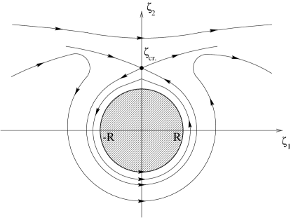
Figure 2: Hydrodynamical picture of the trapping.

Remark 5

In the representation of this hydrodynamical model of the trapping we are forced to choose an orientation of the vortex (see the counterclockwise orientation in fig. 2). However, note that this orientation is irrelevant since it corresponds to the determination of a phase factor that depends on $\phi$, which is not observable at quantum level, in the absence of an appropriate external perturbation.

We are thus naturally led to define the spin–width of the resonance through the uncertainty principle for the angular momentum. This is a very delicate question that has given rise to extensive literature [32]. In fact, no self–adjoint operator exists with all the desiderable properties for an acceptable quantum description of an angular coordinate. If we try to write, in the more conventional form, the standard dispersion inequalities we are led to the paradoxical situation of having an infinite spread in angles for states sharp in angular momentum, while the physical meaning of the angle restricts its values to a finite range. However, this difficulty can be overcome by introducing the exponentials of the angle variables. We proceed as follows: first of all, we fix the canonical variables which come into play. In our case they are: the angular momentum vector ${\bf L}$ and the canonical angle conjugate to $({\bf L}^{2})^{1/2}$, i.e., the angle swept out in the orbital plane.

Remark 6

The use of the $Z$–coordinates allows us to separate the external orbital angular momentum ${\bf L}_{e}$ from the internal orbital angular momentum ${\bf L}_{i}$. In the approximation of our model, we can assume that the internal part of the wavefunction of each cluster is an eigenfunction of ${\bf L}^{2}_{i}$ with null eigenvalue. This is a reasonable approximation in the assumption of spherical clusters, and if we suppose that the tensor forces are of no great relevance. Therefore, the ground state of each cluster can be viewed approximately as an eigenfunction of ${\bf L}^{2}_{i}$ with null eigenvalue. If such approximation holds true, then we only remain with the external orbital angular momentum which can be identified with the vector ${\bf L}$ conjugate to the orbital angle in the sense explained above.

Next, we consider the exponential of the angle $Q=\theta+\frac{\pi}{2}$, i.e., $e^{iQ}$, and the operator ${\bf P}=[({\bf L}^{2}+\frac{1}{4})^{1/2}-\frac{1}{2}]$. Then the minimum uncertainty in the dispersions $\Delta{\bf P}$ and $\Delta(\cos Q)$ is given by (see ref. [32]):

$$\Delta{\bf P}\Delta(\cos Q)=\frac{1}{2}<\sin Q>.$$ (94)

Now consider states that have a sharp value of the observable operator $\cos Q$. The dispersion $\Delta(\cos Q)$ vanishes, and the expectation value $<\sin Q>$ has a finite value. Hence, from the uncertainty relation (94) the dispersion in the angular momentum $\Delta{\bf P}$ becomes unlimitedly large. This behaviour is exactly as would be expected on physical grounds. A maximal sharp angle observable implies a maximally spread value of the angular momentum.

Coming back to our physical problem, we can say that the resonances have a finite lifetime which corresponds to the time of the trapping; after that, the unstable state decays. Then, we can speak of an angular lifetime of the resonance [26] which gives the dispersion in the angle; correspondingly, we shall have a dispersion in the angular momentum as prescribed by the uncertainty relation (94). We thus speak of a spin–width proper of the unstable states, which tends to zero as the angular lifetime tends to infinity. The bound states are, indeed, sharp in the angular momentum.

As explained in section 3, the poles of the resolvent $R_{\ell}(k,g)$ that correspond to the resonances lie in the half–plane ${\mbox{Im}\,}k<0$ (see fig. 1), and their imaginary part is related to the width of the resonance, which is inversely proportional to the time delay. Analogously, we can represent the spin–width of the unstable states by extending the angular momentum to complex values: the dispersion in the angular momentum, prescribed by the uncertainty relation (94), will be represented by the imaginary part of the angular momentum. The latter will be denoted by $\lambda=\alpha+i\beta$. Since the angular momentum is complex, the centrifugal energy is complex too. Neglecting the $\lambda$–dependence proper of the non–local interaction we can write the continuity equation in the following form:

$$\frac{\partial w}{\partial t}+\nabla\cdot{\bf j}=2w\,{\mbox{Im}\,}\left<\frac{\lambda(\lambda+1)}{2\mu R^{2}}\right>,~{}~{}~{}~{}~{}(\hbar=1),$$ (95)

where ${\bf j}$ is the current density (already introduced above), $w=\chi^{*}\chi$, $\mu$ is the reduced mass, and $R$ is the relative distance between the clusters. Then, we have:

$${\mbox{Im}\,}\left<\frac{\lambda(\lambda+1)}{2\mu R^{2}}\right>=\beta(2\alpha+1)\frac{1}{<2\mu R^{2}>}=\frac{\Gamma}{2},$$ (96)

where $\Gamma$ is the width of the resonance. From (96) we get:

$$\Gamma=\frac{\beta(2\alpha+1)}{I},$$ (97)

where $I=<\mu R^{2}>$ is the moment of inertia of the system of clusters, regarded as a rigid rotator. This formula indicates that the values of $\Gamma$ increase for increasing values of $\alpha={\mbox{Re}\,}\lambda$, in perfect agreement with the phenomenological data [3, 4]. This can easily be understood if we observe that, according to the result obtained at the end of section 3, the potentials $V_{\ell}$ become weaker for increasing values of $\ell$, and therefore they cannot sustain the trapping proper of the resonance for a long time. This agrees with the hydrodynamical model, whose condition for producing the trapping (i.e., $\left|\Gamma_{\infty}/4\pi{\bf v}_{\infty}\right|>R$) suggests that at high energies (i.e., high values of $|{\bf v}_{\infty}|$, $\Gamma_{\infty}$ fixed), the trapping is not allowed. In conclusion, $\beta$ can be regarded as the spin–width of the resonance, and its value increases for increasing energy.

This hydrodynamical model, and consequently the spin–width of the resonances, calls for the introduction of the complex angular momentum plane into the description of the rotational band. Describing the resonances by poles moving in the complex plane of the angular momentum (instead of using fixed poles) allows to recover the global character of the rotational bands: i.e., the grouping of resonances in families. This latter method has been successfully used by one of us [GAV] in the phenomenological fits of $\alpha$–$\alpha$, $\alpha$–⁴⁰Ca and $\pi^{+}$–p elastic scattering [33, 34, 35].

Finally, let us note that this approach, giving an increase rate of the resonance width at higher energy, explain the evolution of the rotational resonances into surface waves produced by diffraction, even though at these energies the scenario is quite different, the inelastic scattering and the reaction channels being dominant. At the present time diffraction phenomena and (nuclear and Coulomb) rainbow mainly attract the theoretical and phenomenological attention (see, e.g., refs. [36, 37, 38, 39]). However, it is one of the purposes of this paper to show that a deeper understanding of the evolution, and, accordingly, of the global character of the (low energy) rotational bands can shed light on these high energy phenomena.

Appendix

The results of the spectral analysis reported in section 3 have been completely proved for the case $\ell=0$ in ref. [24], and then partially extended to every integer value of $\ell$ in ref. [25]. This extension is complete if we observe that the proofs for the case $\ell=0$ are based on the following bounds:

$$|kRj_{0}(kR)| = |\sin kR|\leq\frac{2|k|R}{1+|k|R}e^{\alpha r},~{}~{}(|{\mbox{Im}\,}k|\leq\alpha),$$

$$|G_{0}(k;R,R^{\prime})| \leq \frac{2R}{1+|k|R}\,e^{\alpha(R+R^{\prime})},\>~{}~{}({\mbox{Im}\,}k\geq-\alpha),$$

which can easily be extended to any integer value of $\ell$. For the spherical Bessel and Hankel functions the following majorizations hold true [40]:

$$|kRj_{\ell}(kR)| \leq \,\mbox{Const.}\,\left[\frac{|k|R}{1+|k|R}\right]^{(\ell+1)}\,e^{R\,|{\mbox{\small Im}\,}k|},~{}~{}~{}~{}$$ (98)

$$|kRh_{\ell}^{(1)}(kR)| \leq \,\mbox{Const.}\,\left[\frac{1+|k|R}{|k|R}\right]^{\ell}\,e^{-R\,{\mbox{\small Im}\,}k},$$ (99)

the constants depending only on $\ell$. Finally, from (74), (98) and (99) one gets:

$$|kRj_{\ell}(kR)| \leq \,\mbox{Const.}\,\frac{|k|R}{1+|k|R}\,e^{\alpha R},~{}|{\mbox{Im}\,}k|\leq\alpha,~{}~{}~{}~{}~{}$$

$$|G_{\ell}(k;R,R^{\prime})| \leq \,\mbox{Const.}\,\frac{R}{1+|k|R}\,e^{\alpha(R+R^{\prime})},~{}{\mbox{Im}\,}k\geq-\alpha,~{}~{}~{}~{}$$

and these bounds are sufficient for a complete generalization of the spectral results to any integer $\ell$.

References

- [1] K.W. McVoy, in Classical and Quantum Mechanics Aspects of Heavy Ion Collisions, Lecture Notes in Physics 33 (Springer, Berlin, Heidelberg 1974)
- [2] K.W. McVoy, Ann. Phys. 43, 91 (1967)
- [3] S. Okai, S.C. Park, Phys. Rev. 145, 787 (1966)
- [4] K. Langanke, Nucl. Phys. A 377, 53 (1982)
- [5] K. Langanke, R. Stademann, D. Frekers, Phys. Rev. C 29, 40 (1984)
- [6] N. Cindro, D. Počanić, in Resonances Models and Phenomena, Lecture Notes in Physics 211 (Springer, Berlin, Heidelberg 1993), p. 158
- [7] K. Wildermuth, Y.C. Tang, A Unified Theory of the Nucleus, (Vieweg, Braunschweig 1977)
- [8] Y.C. Tang, M. LeMere, D.R. Thompson, Phys. Rep. C 47, 167 (1978)
- [9] M. LeMere, Y.C. Tang, D.R. Thompson, Phys. Rev. C 14, 23 (1976)
- [10] K. Wildermuth, W. McClure, in Springer Tracts in Modern Physics 41 (Springer, Berlin, Heidelberg 1966)
- [11] F. Riesz, B.Sz. Nagy, Leçons d’Analyse Fonctionelle, (Academiai Kiado, Budapest 1953)
- [12] A.J. Dragt, J. Math. Phys. 6, 533 (1965)
- [13] Y.A. Simonov, Sov. J. Nucl. Phys. 3, 461 (1966)
- [14] A.M. Badalayan, Y. A. Simonov, Sov. J. Nucl. Phys. 3, 755 (1966)
- [15] N.I. Vilenkin, Special Functions and the Theory of Group Representations, Transl. Math. Monographs 22, (Amer. Math. Soc., Providence 1968)
- [16] M. Hamermesh, Group Theory, (Addison–Wesley, Reading 1962)
- [17] H. Weyl, The Theory of Groups and Quantum Mechanics, (Dover, New York 1931)
- [18] V. Bargmann, M. Moshinsky, Nucl. Phys. 18, 697 (1960); 23, 177 (1961)
- [19] M. Moshinsky, Y.F. Smirnov, The Harmonic Oscillator in Modern Physics, Contemporary Concepts in Physics 9, (Harwood Academic Publ., Amsterdam 1996)
- [20] J.P. Elliott, Proc. Royal Soc. London A 245 128 (1958)
- [21] J. P. Elliott, The nuclear shell model and its relation with the nuclear models, in Selected Topics in Nuclear Theory, (I.A.E.A., Wien 1963)
- [22] J. Regnier, Nucl. Phys. 54, 225 (1964)
- [23] J. Regnier, Bull. Acad. Roy. Belg. Cl. Sci. 48, 179 (1962)
- [24] M. Bertero, G. Talenti, G.A. Viano, Comm. Math. Phys. 6, 128 (1967)
- [25] M. Bertero, G. Talenti, G. A. Viano, Nucl. Phys. A 115, 395 (1968)
- [26] V. De Alfaro, T. Regge, Potential Scattering, (North–Holland, Amsterdam 1965)
- [27] W. Zickendrath, Ann. Phys. 35, 18 (1965)
- [28] W. Zickendrath, J. Math. Phys. 10, 30 (1969)
- [29] W. Zickendrath, J. Math. Phys. 12, 1663 (1971)
- [30] V. Gallina, P. Nata, L. Bianchi, G.A. Viano, Nuovo Cimento 24, 835 (1962)
- [31] F.T. Smith, J. Math. Phys. 3, 735 (1962)
- [32] L.C. Biedenharn, J.D. Louck, in Encyclopedia of Mathematics and its Applications 9 (Addison–Wesley, Reading 1981), p. 307 (see also the references quoted therein)
- [33] G.A. Viano, Phys. Rev. C 36, 933 (1987)
- [34] G.A. Viano, Phys. Rev. C 37, 1660 (1988)
- [35] R. Fioravanti, G.A. Viano, Phys. Rev. C 55, 2593 (1997)
- [36] H. M. Nussenzveig, Diffraction Effects in Semiclassical Scattering, (Cambridge Univ. Press, Cambridge 1992)
- [37] D. T. Khoa, G. R. Satchler, W. von Oertzen, Phys. Rev. C 56, 954 (1997)
- [38] D. T. Khoa, G. R. Satchler, Nucl. Phys. A 668, 3 (2000)
- [39] W. von Oertzen, D. T. Khoa, H. G. Bohlen, Europhys. News 31/2, 5 (2000); Europhys. News 31/3, 21 (2000)
- [40] R. G. Newton, Phys. Rev. 100, 412 (1955)