Dynamical particle-phonon couplings in proton emission from spherical nuclei

1 Introduction

Although nuclei beyond the proton drip line are unstable against proton emission, their lifetime is sufficiently long to study the spectroscopic properties, because of the fact that the proton has to penetrate the Coulomb barrier. Thanks to the recent experimental developments of production and detection methods, a number of ground-state as well as isomeric proton emitters have recently been discovered. [1, 2] These experimental data have indeed shown that the proton radioactivity provides a powerful tool to study the structure of proton rich nuclei.

In the field of heavy-ion reactions, the coupled-channels formalism has been a standard framework to extract nuclear structure information from experimental data. [3] This formalism has been successfully applied also to deformed proton emitters. [4, 5, 6] For instance, the $\beta_{2}$ deformation parameter of deformed proton emitters has been extracted from the experimental decay widths a/o branching ratios.

In the previous analyses for the proton emitters in the region 68 $<Z<82$, where proton emissions from the 1$h_{11/2}$, 3$s_{1/2}$, and 2$d_{3/2}$ orbitals have been observed, the emitters have been treated as spherical nuclei without any structure. [7] It has been pointed out that such calculations systematically underestimate the measured decay half-lives for proton emissions from the 2$d_{3/2}$ state, while the same model works well for emissions from the 1$h_{11/2}$ and 3$s_{1/2}$ states in both odd-Z even-N and odd-Z odd-N nuclei. [8, 9] For the ¹⁵¹Lu nucleus, this discrepancy was attributed to the effects of oblate deformation of the core nucleus ¹⁵⁰Yb, which alter both the decay dynamics and the spectroscopic factor.  [9, 10, 11] This fact has motivated us to investigate the effects of vibrational excitations on the proton decay of spherical nuclei. [12, 13] Similar effects have been well recognized in the field of heavy-ion subbarrier fusion reactions. [14, 15]

In this contribution, we solve the coupled-channels equations for spherical proton emitters in order to study whether the effects of vibrational excitations of the daughter nucleus consistently account for the measured decay half-life from the 1$h_{11/2}$, 3$s_{1/2}$, and 2$d_{3/2}$ states. In Sect. 2, we briefly review the coupled-channels framework for proton emissions. We use the Green’s function approach to compute the decay rate of resonance states.  [4, 7, 16, 17, 18, 19] We discuss the method both for the one dimensional and for the coupled-channels problems. In Sect. 3.1., we compare our results with the experimental data. We particularly study proton emissions from the 1$h_{11/2}$ and 3$s_{1/2}$ states of ¹⁶¹Re [20] and from the 2$d_{3/2}$ state of ¹⁶⁰Re. [21] A clear vibrational structure in the spectrum of the core nucleus ¹⁶⁰W for the proton emitter ¹⁶¹Re has recently been identified up to the $6^{+}_{1}$ state. [22] We shall assume that the vibrational properties are identical between the core nuclei ¹⁶⁰W and ¹⁵⁹W, and study the sensitivity of the calculated decay rate to the dynamical deformation parameter for the vibration. We will also discuss the dependence on the multipolarity of the phonon state. In Sect. 3.2., we apply the formalism to the proton decay of the ¹⁴⁵Tm nucleus, where the fine structure was recently observed. [23] We then summarize the paper in Sect. 4.

2 Green’s function method for proton radioactivities

2.1 One dimensional case

In this section, we review the method which we use below to calculate the decay rate for proton emissions. Let us first consider the no coupling case. Extension to the coupled-channels problems will be given in the next subsection.

We consider the following Schrödinger equation for a resonance state:

$$\left[-\frac{\hbar^{2}}{2\mu}\frac{d^{2}}{dr^{2}}+\frac{l(l+1)\hbar^{2}}{2\mu r^{2}}+V(r)-\left(E+\frac{i}{2}\mathchar 28928\relax_{0}\right)\right]u(r)=0,$$ (2.1)

where $\mu$ is the reduced mass for the relative motion between the valence proton and the daughter nucleus, and $V(r)$ is a potential which consists of the nuclear, the spin-orbit, and the Coulomb parts. We describe the resonance state using the Gamow wave function. Accordingly, $u(r)$ satisfies the boundary condition that it is regular at the origin and is proportional to the outgoing wave asymptotically, namely

$$u(r) = r^{l+1}\hskip 113.81102pt~{}~{}~{}~{}~{}~{}(r\to 0),$$ (2.2)

$$\to {\cal N}(G_{l}(kr)+iF_{l}(kr))\hskip 42.67912pt~{}~{}~{}~{}(r\to\infty),$$ (2.3)

where $k$ is the wave number, and $F_{l}$ and $G_{l}$ is the regular and the irregular Coulomb wave functions, respectively. As is well known, these boundary conditions cannot be satisfied with a real energy $E$, and an imaginary part of the energy is included in Eq. (2.1). The latter is nothing but the decay width of the resonance state. This quantity is calculated also as a ratio between the asymptotic outgoing flux and the normalization inside the barrier, [6]

$$\mathchar 28928\relax_{0}=\frac{\hbar^{2}k}{\mu}{\cal N}^{2}\left/\int^{r_{t}}_{0}\,|u(r)|^{2}\,dr\right.,$$ (2.4)

where $r_{t}$ is the outermost turning point.

An alternative approach to calculate the decay width $\mathchar 28928\relax_{0}$ has been proposed, which is based on the Green’s function formalism. [4, 7, 16, 17, 18, 19] This method was first developed for $\alpha$ decays by Kadmensky and his collaborators [16] and was recently applied to the coupled-channels problem for deformed proton emitters by Esbensen and Davids.  [4]

In this method, one first sets $\mathchar 28928\relax_{0}$ to be 0 in Eq. (2.1) and looks for a standing wave solution which has an asymptotic form of

$$\phi(r)\to{\cal\widetilde{N}}G_{l}(kr)\hskip 56.9055pt~{}~{}~{}~{}(r\to\infty).$$ (2.5)

The coefficient ${\cal\widetilde{N}}$ is determined so that the wave function $\phi$ is normalized to one inside the barrier. Note that $\phi$ corresponds to the solution where the nuclear phase shift is equal to $\pi$/2. This procedure should be a good approximation since $\mathchar 28928\relax_{0}$ is extremely smaller than the real part of the energy $E$ (typically $\mathchar 28928\relax_{0}$ is between 10^-18 and 10^-22MeV while $E$ is order of MeV). [2] The next step is to apply the Gell-Mann-Goldberger transformation [24] to the total Schrödinger equation $[\hat{T}-(E+i\mathchar 28928\relax_{0}/2)]\mathchar 28937\relax=-V\mathchar 28937\relax$, where $\hat{T}$ is the kinetic energy operator. Adding the point Coulomb potential $V_{C}(r)=Z_{D}e^{2}/r$, $Z_{D}$ being the charge number of the daughter nucleus, to both the left and the right hand sides, this equation is transformed to

$$\left[\hat{T}+\frac{Z_{D}e^{2}}{r}-\left(E+\frac{i\mathchar 28928\relax_{0}}{2}\right)\right]\mathchar 28937\relax=\left(\frac{Z_{D}e^{2}}{r}-V(r)\right)\mathchar 28937\relax.$$ (2.6)

The formal solution of this equation reads

$$\mathchar 28937\relax=\frac{1}{\hat{T}+\frac{Z_{D}e^{2}}{r}-\left(E+\frac{i\mathchar 28928\relax_{0}}{2}\right)}\left(\frac{Z_{D}e^{2}}{r}-V(r)\right)\mathchar 28937\relax.$$ (2.7)

Next two approximations are made. Firstly one replaces $\mathchar 28937\relax$ on the right hand side of Eq. (2.7) with the standing wave solution $\mathchar 28936\relax$, whose radial part satisfies the boundary condition given by Eq. (2.5). Secondly, one regards $\mathchar 28928\relax_{0}/2$ as an infinitesimal number $\eta$ which provides the outgoing wave boundary condition for the single particle Green’s function $(\hat{T}+V_{C}-E-i\eta)^{-1}$. As long as $\mathchar 28928\relax_{0}$ is extremely small compared with $E$, its actual value is not important at this stage. As is well known, the single particle Green’s function is expressed in terms of the regular and the outgoing wave functions as [19]

$$\left\langle\mbox{\boldmath$r$}\left|\frac{1}{\hat{T}+V_{C}-E-i\eta}\right|\mbox{\boldmath$r$}^{\prime}\right\rangle=\sum_{l,m}\frac{2\mu}{k\hbar^{2}}\frac{O_{l}(kr_{>})}{r_{>}}\frac{F_{l}(kr_{<})}{r_{<}}{\cal Y}_{jlm}(\hat{\mbox{\boldmath$r$}}_{>}){\cal Y}_{jlm}^{*}(\hat{\mbox{\boldmath$r$}}_{<}),$$ (2.8)

where $O_{l}=G_{l}+iF_{l}$ is the outgoing Coulomb wave. One then obtains[19]

$$\mathchar 28937\relax(\mbox{\boldmath$r$}) = \int\,d\mbox{\boldmath$r$}^{\prime}\left\langle\mbox{\boldmath$r$}\left|\frac{1}{\hat{T}+V_{C}-E-i\eta}\right|\mbox{\boldmath$r$}^{\prime}\right\rangle\left\langle\mbox{\boldmath$r$}^{\prime}\left|\left(\frac{Z_{D}e^{2}}{r^{\prime}}-V(r^{\prime})\right)\right.\right.\mathchar 28936\relax,$$ (2.9)

$$= \frac{2\mu}{k\hbar^{2}}\frac{O_{l}(kr)}{r}{\cal Y}_{jlm}(\hat{r})\int^{\infty}_{0}dr^{\prime}\,F_{l}(kr^{\prime})\left(\frac{Z_{D}e^{2}}{r^{\prime}}-V(r^{\prime})\right)\phi(r^{\prime}),$$ (2.10)

as $r\to\infty$. From this equation, the normalization factor ${\cal N}$ in Eq. (2.3) is found to be

$${\cal N}=\frac{2\mu}{k\hbar^{2}}\int^{\infty}_{0}dr^{\prime}\,F_{l}(kr^{\prime})\left(\frac{Z_{D}e^{2}}{r^{\prime}}-V(r^{\prime})\right)\phi(r^{\prime}).$$ (2.11)

The decay rate is then obtained by Eq. (2.4), by replacing $u(r)$ with $\phi(r)$ in the denominator.

2.2 Coupled-channels problem

Let us now discuss the channel coupling effects on proton radioactivities of spherical nuclei. In order to take into account the vibrational core excitations, we consider the following Hamiltonian:

$$H=-\frac{\hbar^{2}}{2\mu}\nabla^{2}+V(r)+V_{\rm coup}(\mbox{\boldmath$r$},\alpha)+H_{\rm vib},$$ (2.12)

where $\alpha$ is the coordinate for the vibrational phonon of the daughter nucleus. It is related to the dynamical deformation parameter as $\alpha_{\lambda\mu}=\frac{\beta_{\lambda}}{\sqrt{2\lambda+1}}(a_{\lambda\mu}^{\dagger}+(-)^{\mu}a_{\lambda\mu})$, where $\lambda$ is the multipolarity of the vibrational mode and $a_{\lambda\mu}^{\dagger}(a_{\lambda\mu})$ is the creation (annihilation) operator of the phonon. $H_{\rm vib}=\hbar\omega\sum_{\mu}a_{\lambda\mu}^{\dagger}a_{\lambda\mu}$ is the Hamiltonian for the vibrational phonon. In this paper, for simplicity, we do not consider the possibility of multi-phonon excitations, but include only excitations to the single phonon state. The coupling Hamiltonian $V_{\rm coup}(\mbox{\boldmath$r$},\alpha)$ consists of three terms, i.e., $V_{\rm coup}(\mbox{\boldmath$r$},\alpha)=V_{\rm coup}^{(N)}(\mbox{\boldmath$r$},\alpha)+V_{\rm coup}^{(ls)}(\mbox{\boldmath$r$},\alpha)+V_{\rm coup}^{(C)}(\mbox{\boldmath$r$},\alpha)$. The nuclear term reads

$$V_{\rm coup}^{(N)}(\mbox{\boldmath$r$},\alpha)=-\frac{V_{0}}{1+\exp\left(\frac{r-R_{0}-R_{0}\,\alpha_{\lambda}\cdot Y_{\lambda}(\hat{\mbox{\boldmath$r$}})}{a}\right)}-V_{N}(r)\,,$$ (2.13)

where the dot denotes a scalar product. We have assumed that the nuclear potential is given by the Woods-Saxon form. $V_{N}(r)$ is the nuclear component of the bare potential $V(r)$. This term is subtracted in order to avoid the double counting. Notice that we do not expand the nuclear coupling potential but include the couplings to the all orders with respect to the phonon operator.  [3, 25] The matrix elements of this coupling Hamiltonian are evaluated using a matrix algebra, as in Ref. ?. As for the Coulomb $V_{\rm coup}^{(C)}$ as well as the spin-orbit $V_{\rm coup}^{(ls)}$ terms, the effects of higher order couplings are expected to be small, [25] and we retain only the linear term. The Coulomb term thus reads

$$V_{\rm coup}^{(C)}(\mbox{\boldmath$r$},\alpha) = \frac{3Z_{D}e^{2}}{r}\,\frac{1}{2\lambda+1}\left(\frac{R_{c}}{r}\right)^{\lambda}\alpha_{\lambda}\cdot Y_{\lambda}(\hat{\mbox{\boldmath$r$}})~{}~{}~{}~{}~{}~{}({\rm for}~{}r>R_{c})$$ (2.14)

$$= \frac{3Z_{D}e^{2}}{R_{c}}\,\frac{1}{2\lambda+1}\left(\frac{r}{R_{c}}\right)^{\lambda}\alpha_{\lambda}\cdot Y_{\lambda}(\hat{\mbox{\boldmath$r$}})~{}~{}~{}~{}~{}~{}({\rm for}~{}r\leq R_{c}),$$ (2.15)

where $R_{c}$ is the charge radius. For the spin-orbit interaction, we express it in the so called Thomas form, [4, 26]

$$V_{\rm coup}^{(ls)}(\mbox{\boldmath$r$},\alpha)=V_{\rm so}\frac{1}{r}\,\frac{df}{dr}\,\mbox{\boldmath$l$}\cdot\mbox{\boldmath$\sigma$}+i\,V_{\rm so}R_{\rm so}\sum_{\mu}\alpha_{\lambda\mu}^{*}\left\{\left(\nabla\frac{df}{dr}Y_{\lambda\mu}(\hat{\mbox{\boldmath$r$}})\right)\cdot\left(\nabla\times\mbox{\boldmath$\sigma$}\right)\right\}\,,$$ (2.16)

where $f(r)=1/[1+\exp((r-R_{\rm so})/a_{\rm so})]$. The last term in Eq. (2.16) can be decomposed to a sum of angular momentum tensors using a formula [27]

$$\left(\nabla g(r)Y_{\lambda\mu}(\hat{\mbox{\boldmath$r$}})\right)\cdot\mbox{\boldmath$C$} = -\sqrt{\frac{\lambda+1}{2\lambda+1}}\left(\frac{dg}{dr}-\frac{\lambda}{r}\,g(r)\right)[Y_{\lambda+1}\mbox{\boldmath$C$}]^{(\lambda\mu)}$$ (2.17)

$$+\sqrt{\frac{\lambda}{2\lambda+1}}\left(\frac{dg}{dr}+\frac{\lambda+1}{r}\,g(r)\right)[Y_{\lambda-1}\mbox{\boldmath$C$}]^{(\lambda\mu)}.$$

In order to solve the coupled-channels equations, we expand the total wave function as

$$\mathchar 28937\relax_{jm}(\mbox{\boldmath$r$},\alpha)=\sum_{l_{p}j_{p}}\sum_{nI}\frac{u^{(j)}_{l_{p}j_{p}nI}(r)}{r}\,|(l_{p}j_{p}nI)jm\rangle,$$ (2.18)

where

$$\langle\hat{\mbox{\boldmath$r$}},\alpha|(l_{p}j_{p}nI)jm\rangle=\sum_{m_{p}m_{I}}\langle j_{p}m_{p}Im_{I}|jm\rangle{\cal Y}_{j_{p}l_{p}m_{p}}(\hat{\mbox{\boldmath$r$}})\varphi_{nIm_{I}}(\alpha),$$ (2.19)

$\varphi$ being the vibrational wave function. The coupled-channels equations are obtained by projecting out the intrinsic state $|(l_{p}j_{p}nI)jm\rangle$ from the total Schrödinger equation, and read

$$\left[-\frac{\hbar^{2}}{2\mu}\frac{d^{2}}{dr^{2}}+\frac{l_{p}(l_{p}+1)\hbar^{2}}{2\mu r^{2}}+V(r)-\left(E+\frac{i}{2}\mathchar 28928\relax_{0}\right)+n\hbar\omega\right]u^{(j)}_{l_{p}j_{p}nI}(r)$$

$$\hskip 71.13188pt=-\sum_{l_{p}^{\prime}j_{p}^{\prime}}\sum_{n^{\prime}I^{\prime}}\langle(l_{p}j_{p}nI)jm|V_{\rm coup}|(l_{p}^{\prime}j_{p}^{\prime}n^{\prime}I^{\prime})jm\rangle u^{(j)}_{l_{p}^{\prime}j_{p}^{\prime}n^{\prime}I^{\prime}}(r)$$ (2.20)

To solve these equations, one needs to compute the coupling matrix elements of the operators $\alpha_{\lambda}\cdot T_{\lambda}$, where $T_{\lambda\mu}$ is either $Y_{\lambda\mu}$ or $[Y_{\lambda\pm 1}\,(-i\,\nabla\times\mbox{\boldmath$\sigma$})]^{(\lambda\mu)}$. These are expressed in terms of the Wigner’s 6-j symbol as [27]

$$\langle(l_{p}^{\prime}j_{p}^{\prime}n^{\prime}I^{\prime})jm|\alpha_{\lambda}\cdot T_{\lambda}|(l_{p}j_{p}nI)jm\rangle = (-)^{j_{p}+I^{\prime}+j}\left\{\matrix{j&I^{\prime}&j_{p}^{\prime}\cr\lambda&j_{p}&I\cr}\right\}$$ (2.21)

$$\times\langle{\cal Y}_{j_{p}^{\prime}l_{p}^{\prime}}||T_{\lambda}||{\cal Y}_{j_{p}l_{p}}\rangle\,\langle\phi_{n^{\prime}I^{\prime}}||\alpha_{\lambda}||\phi_{nI}\rangle.$$

For transitions between the ground and the one phonon states which we consider in this paper, the reduced matrix element $\langle\phi_{n^{\prime}I^{\prime}}||\alpha_{\lambda}||\phi_{nI}\rangle$ is given by $\beta_{\lambda}$. The reduced matrix elements for the operators $T_{\lambda}$ are found in Ref. ?.

The Green’s function method discussed in the previous subsection can provide a convenient way to calculate the decay width particularly for the coupled-channels problems. [4] The direct method seeks the Gamow wave functions where $u^{(j)}_{l_{p}j_{p}nI}(r)$ have the asymptotic form of ${\cal N}^{(j)}_{l_{p}j_{p}nI}(G_{l_{p}}(k_{nI}r)+i\,F_{l_{p}}(k_{nI}r))$ at $r\to\infty$ for all the channels, where $k_{nI}=\sqrt{2\mu(E-n\hbar\omega)/\hbar^{2}}$ is the channel wave number. This method, however, requires to solve the coupled-channels equations in the complex energy plane and out to large distances, which is quite time consuming and also may be difficult to obtain accurate solutions. In the Green’s function method, in contrast, the coupled-channels equations are solved in the real energy plane and the solutions are matched to the irregular Coulomb wave functions $G_{l_{p}}$ at a relatively small distance $r_{\rm match}$, which is outside the range of nuclear couplings. From the solution of the coupled-channels equations $\mathchar 28937\relax^{cc}_{jm}(\mbox{\boldmath$r$},\alpha)$ thus obtained, the outgoing wave function for the resonance Gamow state is generated using the Coulomb propagator as [4, 19]

$$\mathchar 28937\relax_{jm}(\mbox{\boldmath$r$},\alpha) = -\int d\mbox{\boldmath$r$}^{\prime}d\alpha^{\prime}\left\langle\mbox{\boldmath$r$}\alpha\left|\frac{1}{H_{\rm coul}+H_{\rm vib}-E-i\eta}\right|\mbox{\boldmath$r$}^{\prime}\alpha^{\prime}\right\rangle$$ (2.22)

$$\times \left(V(r^{\prime})+V_{\rm coup}(\mbox{\boldmath$r$}^{\prime},\alpha^{\prime})-\frac{Z_{D}e^{2}}{r^{\prime}}\right)\mathchar 28937\relax^{cc}_{jm}(\mbox{\boldmath$r$}^{\prime},\alpha^{\prime}),$$

where $H_{\rm coul}=-\hbar^{2}\nabla^{2}/2\mu+Z_{D}e^{2}/r$ is the Hamiltonian for the point Coulomb field. As in the previous subsection, the asymptotic normalization factors ${\cal N}^{(j)}_{l_{p}j_{p}nI}$ are found to be [4]

$${\cal N}^{(j)}_{l_{p}j_{p}nI} = -\frac{2\mu}{\hbar^{2}k_{nI}}\int^{\infty}_{0}dr\,rF_{l_{p}}(k_{nI}r)$$ (2.24)

$$\times\left\langle(l_{p}j_{p}nI)jm\left|V(r)+V_{coup}(\mbox{\boldmath$r$},\alpha)-\frac{Z_{D}e^{2}}{r}\right|\mathchar 28937\relax^{cc}_{jm}\right\rangle,$$

$$= -\frac{2\mu}{\hbar^{2}k_{nI}}\int^{\infty}_{0}dr\,F_{l_{p}}(k_{nI}r)\left\{\left(V(r)-\frac{Z_{D}e^{2}}{r}\right)u_{l_{p}j_{p}nI}(r)\right.$$

$$+\left.\sum_{l_{p}^{\prime}j_{p}^{\prime}}\sum_{n^{\prime}I^{\prime}}\langle(l_{p}j_{p}nI)jm|V_{\rm coup}|(l_{p}^{\prime}j_{p}^{\prime}n^{\prime}I^{\prime})jm\rangle u^{(j)}_{l_{p}^{\prime}j_{p}^{\prime}n^{\prime}I^{\prime}}(r)\right\}$$

In this way, the effects of the long range Coulomb couplings outside the matching radius $r_{\rm match}$ are treated perturbatively. The partial decay width is then calculated as $\mathchar 28928\relax_{l_{p}j_{p}nI}=\hbar^{2}k_{nI}|{\cal N}^{(j)}_{l_{p}j_{p}nI}|^{2}/\mu$, provided that the wave function $\mathchar 28937\relax^{cc}_{jm}$ is normalized inside the outer turning point.

3 Comparison with experimental data

We now solve the coupled-channels equations and compare the results with the experimental data. One of the most important experimental observables is the decay half-life. In the present framework, it is calculated as

$$T_{1/2}=\frac{\hbar}{S_{j}\mathchar 28928\relax_{j}}\ln 2,$$ (3.1)

where $S_{j}$ is the spectroscopic factor for the resonance state, which takes into account correlations beyond the single-particle picture. If one assumes that the ground state of an odd-Z nucleus is a one-quasiparticle state, the spectroscopic factor $S_{j}$ is identical to the unoccupation probability for this state and is given by $S_{j}=u_{j}^{2}$ in the BCS approximation. [7]

In all the calculations in this section, we use the real part of the Becchetti-Greenless optical model potential for the proton-daughter nucleus potential. [29] The potential depth was adjusted so as to reproduce the experimental proton decay $Q$ value for each value of the dynamical deformation parameter $\beta$ and the excitation energy $\hbar\omega$ of the vibrational phonon excitations in the daughter nucleus. Following Ref. ?, we assume that the depth of the spin-orbit potential is related to that of the central potential by $V_{\rm so}=-0.2V_{0}$. The charge radius $R_{c}$ is assumed to be the same as $R_{0}$ in the nuclear potential. The spectroscopic factor $S_{j}$ in Eq. (3.1) is taken from Ref. ?. This was evaluated in the BCS approximation to a monopole pairing Hamiltonian for single-particle levels obtained with a spherical Woods-Saxon potential.

3.1 ^160,161Re nuclei: reconciliation of the $d_{3/2}$ puzzle

In this subsection, we solve the coupled-channels equations for the resonant 1$h_{11/2}$ and 3$s_{1/2}$ states in ¹⁶¹Re as well as the 2$d_{3/2}$ state in ¹⁶⁰Re. The first 2⁺ state in the core nucleus ¹⁶⁰W for the ¹⁶¹Re nucleus was recently observed at $\hbar\omega_{2}=$610 keV. [22]Accordingly we first discuss the effects of the quadrupole vibrational excitations. Figure 1 shows the dependence of the decay half-life for proton emissions from the three resonance states on the dynamical deformation parameter $\beta_{2}$ of the quadrupole mode. The experimental values for the decay half-life are taken from Refs. ?, ?, and are denoted by the dashed lines. The arrows are the half-lives in the absence of the vibrational mode. For the decays from the 3$s_{1/2}$ and 1$h_{11/2}$ states, if one takes into account uncertainty in the experimental $Q$ value of the proton emission, these calculations for the decay half-life in the no coupling limit are within the experimental error bars. [7] In clear contrast, the calculation for the 2$d_{3/2}$ state is still off from the experimental data by about 30% even when uncertainty of the decay $Q$ value is taken into consideration. [7]

The results of the coupled-channels calculations are shown by the solid lines in the figure. We treat the extra neutron as a spectator for the odd-odd proton emitter ¹⁶⁰Re. One notices that the channel coupling effects significantly enhance the decay half-life for the 2$d_{3/2}$ state, while the effects are more marginal for the 3$s_{1/2}$ and

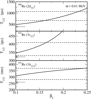
Fig. 1: The decay half-lives for proton emission from the 2$d_{3/2}$ state of ¹⁶⁰Re and the 3$s_{1/2}$ and 1$h_{11/2}$ states of ¹⁶¹Re as a function of the dynamical deformation parameter $\beta_{2}$ of the quadrupole vibrational excitation of the daughter nuclei. The vibrational excitation energy is $\hbar\omega_{2}$ = 0.61 MeV. The experimental data are taken from Refs. 20) and 21) and are denoted by the dashed lines. The arrows indicate the results in the no coupling limit.

 

1$h_{11/2}$ states (notice the difference of the scale of the vertical axis in the figure). Our results show that all of the three half-lives can be reproduced simultaneously if the dynamical deformation parameter is around $\beta_{2}\sim 0.16$.

Why is only the $d_{3/2}$ state affected considerably by the channel coupling effects while the others are not? A possible explanation is as follows. The quadrupole interaction mixes the $s$ and $d$ states. For the $s_{1/2}$ state, a small admixture of $d$ states does not affect much, since the decay from the $|s_{1/2}\otimes 0^{+}\rangle$ state dominates after all. On the other hand, for the $d_{3/2}$ state, a small admixture of $s$ state can influence the decay dynamics significantly depending on the excitation energy: there is no centrifugal barrier for the $|s_{1/2}\otimes 2^{+}\rangle$ state, and thus the decay from this component can compete with the decay from the dominant component $|d_{3/2}\otimes 0^{+}\rangle$ state even though the energy for the relative motion is smaller. For the $h_{11/2}$ state, the quadrupole interaction mixes it with the $|f_{7/2}\otimes 2^{+}\rangle$ component. The decay from the latter may compete with the decay from the main component due to the smaller centrifugal potential. Compared with the $d_{3/2}$ state, however, the effective proton energy in the incident channel defined as $E_{p}^{eff}=E_{p}-V_{\rm cent}(r)-V(r)$ is smaller, which makes the channel coupling effects weaker. Therefore, the core excitations do not influence significantly the proton decay from the $h_{11/2}$ state unless the coupling is very large a/o the excitation energy is very small.

Let us now discuss the dependence of the decay rate on the multipolarity of the phonon mode. Figure 2 shows the effects of octupole phonon excitations on the decay half-life from the 2$d_{3/2}$ state of ¹⁶⁰Re. As an illustrative example, we take $\hbar\omega_{3}$=0.2 MeV, but results are qualitatively the same for different values of $\hbar\omega_{3}$. For the octupole vibration, the enhancement of the half-life is too small to account for the observed discrepancy between the experimental decay half-life and the prediction of the potential model with no coupling. As was noted before, [2] the proton decay is very sensitive to the angular momentum of the proton state. The same seems to be true for the multipolarity of the collective excitation of the daughter nucleus.

3.2 ¹⁴⁵Tm nucleus: fine structure

We next discuss the fine structure in proton emission from the ¹⁴⁵Tm nucleus, which was recently observed at the Oak Ridge National Laboratory. [23] In the experiment, two clear peaks were seen in the energy spectrum of the emitted proton, one corresponding to the transition from the 1$h_{11/2}$ state in ¹⁴⁵Tm to the ground state of the daughter nucleus ¹⁴⁴Er and the other to the first excited state at 0.326 MeV. The measured ground state decay half-life was 3.1$\pm 0.3\mu$s, and the branching ratio

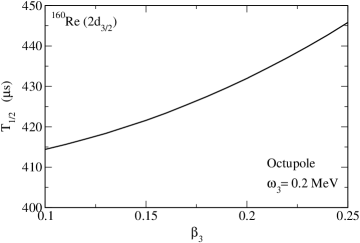
Fig. 2: The decay half-life for proton emission from the 2$d_{3/2}$ state of ¹⁶⁰Re as a function of the dynamical deformation parameter of the octupole phonon excitation of the core nucleus. The excitation energy is set to be 0.2 MeV.

 

was 9.6$\pm$1.5%. [23] Davids and Esbensen have made a detailed analysis for the fine structure of this decay mode using the particle-vibration coupling model. [13] They obtained good agreement with the data for both the half-life and the branching ratio. Figure 3 shows results with our model Hamiltonian, which is slightly different from the one used by Davids and Esbensen (e.g., we include the coupling Hamiltonian for the spin-orbit interaction as well). The experimental data are denoted by the dot-dashed lines. The three theoretical curves are for three different proton energies, taking its experimental uncertaintity into consideration. We find that the ground state half-life and the branching ratio are simultaneously reproduced if the dynamical deformation parameter $\beta_{2}$ is larger than 0.22, although more studies on the dependence of the observables on the strength of the spin-orbit interaction $V_{\rm so}$ would be needed in order to extract a more conclusive value of $\beta_{2}$. Our results indicate that the $|f_{7/2}\otimes 2^{+}\rangle$ state admixes 1.08% in probability with the main component $|h_{11/2}\otimes 0^{+}\rangle$ state at $\beta_{2}=0.18$. This is consistent with the experimental suggestion given in Ref.?.

4 Summary

We have solved the coupled-channels equations to take into account the effects of the vibrational excitations of the spherical daughter nucleus during the proton emission. Applying the formalism to the the resonant 1$h_{11/2}$ and 3$s_{1/2}$ states in ¹⁶¹Re and the 2$d_{3/2}$ state in ¹⁶⁰Re, we have found that the experimental data for the decay half-lives for these three states can be reproduced simultaneously if the quadrupole phonon excitation with $\beta_{2}\sim 0.16$ is considered. This removes the discrepancy observed before between the experimental data and the prediction of the optical potential model calculation for the decaying 2$d_{3/2}$ state in this mass region without destroying the agreement for the 1$h_{11/2}$ and 3$s_{1/2}$ states. A similar calculation with the octupole phonon was not satisfactory. We also discussed the fine structure in proton emission of ¹⁴⁵Tm nucleus. The experimental data for the half-life as well as the branching ratio were simultaneously reproduced within our model, with a reasonable admixture of the excited state components in the total wave function.

The previous coupled-channels analyses were restricted to deformed proton emitters. Our studies indicate that the channel coupling effects are significant also for spherical emitters. Combining with the previous results, our analyses show that all the observed proton emitters can now be described in a simple single particle picture provided that the collective motion of the daughter nucleus is taken into account.

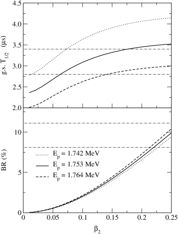
Fig. 3: Sensitivity of the decay half-life (the upper panel) and the branching ratio (the lower panel) for the proton emission of ¹⁴⁵Tm to the dynamical deformation parameter $\beta_{2}$ of the quadrupole phonon excitation of the daughter nucleus ¹⁴⁴Er.

References

- [1] Proceedings of the first international symposium on Proton-Emitting Nuclei PROCON ’99, edited by J.C. Batchelder, AIP Conference Proceedings vol. 518 (American Institute of Physics, New York, 2000), and references there in.
- [2] P.J. Woods and C.N. Davids, Annu. Rev. Nucl. Part. Sci. 47, 541 (1997).
- [3] K. Hagino, N. Rowley, and A.T. Kruppa, Comp. Phys. Comm. 123, 143 (1999).
- [4] H. Esbensen and C.N. Davids, Phys. Rev. C63, 014315 (2000).
- [5] A.T. Kruppa, B. Barmore, W. Nazarewicz, and T. Vertse, Phys. Rev. Lett. 84, 4549 (2000); B. Barmore, A.T. Kruppa, W. Nazarewicz, and T. Vertse, Phys. Rev. C62, 054315 (2000).
- [6] E. Maglione, L.S. Ferreira, and R.J. Liotta, Phys. Rev. Lett. 81, 538 (1998); Phys. Rev. C59, R589 (1999).
- [7] S. Åberg, P.B. Semmes, and W. Nazarewicz, Phys. Rev. C56, 1762 (1997); ibid C58, 3011 (1998).
- [8] C.N. Davids et al., Phys. Rev. C55, 2255 (1997).
- [9] C.R. Bingham et al., Phys. Rev. C59, R2984 (1999).
- [10] L.S. Ferreira and E. Maglione, Phys. Rev. C61, 021304(R) (2000).
- [11] P.B. Semmes, Nucl. Phys. A682, 239c (2001).
- [12] K. Hagino, Phys. Rev. C64, 041304(R) (2001).
- [13] C.N. Davids and H. Esbensen, Phys. Rev. C64, 034317 (2001).
- [14] M. Dasgupta, D.J. Hinde, N. Rowley, and A.M. Stefanini, Annu. Rev. Nucl. Part. Sci., 48, 401 (1998).
- [15] A.M. Stefanini et al., Phys. Rev. Lett. 74, 864 (1995).
- [16] S.G. Kadmensky, V.E. Kalechtis, and A.A. Martynov, Sov. J. Nucl. Phys. 14, 193 (1972); S.G. Kadmensky and V.G. Khlebostroev, Sov. J. Nucl. Phys. 18, 505 (1974).
- [17] V.P. Bugrov, S.G. Kadmensky, V.I. Furman, and V.G. Khlebostroev, Sov. J. Nucl. Phys. 41, 717 (1985).
- [18] V.P. Bugrov and S.G. Kadmensky, Sov. J. Nucl. Phys. 49, 967 (1989); S.G. Kadmensky and V.P. Bugrov, At. Nucl. 59, 399 (1996).
- [19] C.N. Davids and H. Esbensen, Phys. Rev. C61, 054302 (2000).
- [20] R.J. Irvine et al., Phys. Rev. C55, R1621 (1997).
- [21] R.D. Page et al., Phys. Rev. Lett. 68, 1287 (1992).
- [22] A. Keenan et al., Phys. Rev. C63, 064309 (2001).
- [23] K.P. Rykaczewski et al., Nucl. Phys. A682, 270c (2001); K.P. Rykaczewski (private communication).
- [24] N.K. Glendenning, Direct Nuclear Reactions (Academic, New York, 1983), p. 49.
- [25] K. Hagino, N. Takigawa, M. Dasgupta, D.J. Hinde, and J.R. Leigh, Phys. Rev. C55, 276 (1997).
- [26] G.R. Satchler, Direct Nuclear Reaction, (Oxford University Press, Oxford, 1983), p. 622.
- [27] A.R. Edmonds, Angular Momenta in Quantum Mechanics, (Princeton University Press, Princeton N.J., 1957), Eqs. (5.9.17) and (7.1.6).
- [28] P.-G. Reinhard and Y.K. Gambhir, Ann. der Physik (Leipzig) 1, 598 (1992).
- [29] F.D. Becchetti and G.W. Greenless, Phys. Rev. 182, 1190 (1969).