Echos of the liquid-gas phase transition in multifragmentation

Abstract

A general discussion is made concerning the ways in which one can get signatures about a possible liquid-gas phase transition in nuclear matter. Microcanonical temperature, heat capacity and second order derivative of the entropy versus energy formulas have been deduced in a general case. These formulas are exact, simply applicable and do not depend on any model assumption. Therefore, they are suitable to be applied on experimental data. The formulas are tested in various situations. It is evidenced that when the freeze-out constraint is of fluctuating volume type the deduced (heat capacity and second order derivative of the entropy versus energy) formulas will prompt the spinodal region through specific signals. Finally, the same microcanonical formulas are deduced for the case when an incomplete number of fragments per event are available. These formulas could overcome the freeze-out backtracking deficiencies.

,

1 Introduction

From a long time it is believed that, due to the van der Waals nature of the nucleon-nucleon interaction, nuclear matter is likely to exhibit a liquid-gas phase transition [1]. While such a phase transition was predicted within various models, from the experimental point of view so far things are rather inconclusive. The reasons are related to both the inherent difficulties of backtracking the freeze-out stage and the lack of any rigorous mathematical apparatus permitting the unambiguous determination of a liquid-gas phase transition when it exists in experimental data. Some years ago, the general conviction was that the experimental measurement of the nuclear caloric curve could give a definite answer to this problem. Neglecting the weaknesses of each of the “thermometers” tested with that occasion, there is one fundamental barrier preventing the inference of a first order phase transition from any experimentally obtained caloric curve even with back-bending shape: The experimentally obtained microcanonical systems follow an unknown path in the excitation energy ($E$)- freeze-out volume ($V$) plane [2]. Even if the experimental path intersects the coexistence region the phase transition may remain unrevealed in the caloric curve [2]. For overcoming that situation it was proposed that the heat capacity being a quantity independent on the experimental path but depending on the local freeze-out constrain could give precise information concerning the occurrence of the transition [3, 2]. More exactly, if the experimental path is intersecting the spinodal region of the system’s phase diagram, this would be signaled by a negative value of the heat capacity. An analytical heat capacity formula was proposed with that occasion and was subsequently employed in investigating the experimental data obtained by the MULTICS-MINIBALL collaboration occasion with which negative branches of the heat capacity curves were identified [4]. The formula was further applied on the INDRA data with the same success [5]. However, it is worth noticing that though formally correctly deduced, this formula is based on unevaluated terms (such as the microcanonical temperature ($T$) or the heat capacity ($C_{1}$) corresponding to a partial energy of the system ($E_{1}$)) which further imply a chain of assumptions and approximations resulting in (unpredicted) deviations from the exact results.

The above matters motivated us to draw the attention in the present paper on an alternate way to calculate the microcanonical heat capacity of nuclear systems proposed in Ref. [6]. As will be further shown this method is exact, model independent, simply applicable and does not depend on any unevaluated term. The present paper is structured as follows: Section 2 gives a brief review of the model used for illustrating the paper’s ideas. Section 3 investigates on the possible signals one can (experimentally) get about a possible liquid-gas phase transition. Microcanonical formulas for temperature, heat capacity and second-order derivative of the entropy versus energy are deduced for various conservation options in section 4. Examples for the functioning of the above-mentioned formulas are given in section 5. The same quantities are deduced in section 6 for the case in which only a percent of the total number of fragments are available per event. Conclusions are drawn in section 7.

2 Model review

For testing the paper’s argumentation we use the sharp microcanonical multifragmentation model proposed in Ref. [7]. The model concerns the disassembly of a statistically equilibrated nuclear source $(A,Z,E,V)$ (i.e. the source is defined by the parameters: mass number, atomic number, excitation energy, and freeze-out volume respectively); its basic hypothesis is equal probability between all configurations $C:\{A_{i},~{}Z_{i},~{}\epsilon_{i},~{}{\bf r}_{i},~{}{\bf p}_{i},~{}~{}i=1,\dots,N\}$ (the mass number, the atomic number, the excitation energy, the position and the momentum of each fragment $i$ of the configuration $C$, composed of $N$ fragments) which are subject to standard microcanonical constraints: $\sum_{i}A_{i}=A$, $\sum_{i}Z_{i}=Z$, $\sum_{i}{\bf p}_{i}=0$, $\sum_{i}{\bf r}_{i}\times{\bf p}_{i}=0$, $E$ - constant; integration over the fragments’ momenta can be analytically performed in the expression of the total number of states, then one works in the smaller configuration space: $C^{\prime}:\{A_{i},~{}Z_{i},~{}\epsilon_{i},~{}{\bf r}_{i},~{}~{}i=1,\dots,N\}$; a Metropolis-type simulation is employed for determining the average value of any system observable. Function of the desired conservation restriction (${\mathcal{R}}$) level ($n$) one can write:

$$W_{C^{\prime}}\propto I_{p}=\int\prod_{i=1}^{N}{\rm d}{\bf p}_{i}~{}{\mathcal{R}}(n)=\frac{2\pi\prod_{i}m_{i}^{3/2}}{\Gamma\left(\frac{3}{2}(N-n)\right)}f(n)\left(2\pi K\right)^{\frac{3}{2}(N-n)-1},$$ (1)

with $n=0,1,2$; ${\mathcal{R}}(0)=\delta\left(H-E\right)$, ${\mathcal{R}}(1)={\mathcal{R}}(0)~{}\delta\left(\sum_{i}{\bf p}_{i}\right)$, ${\mathcal{R}}(2)={\mathcal{R}}(1)~{}\delta\left(\sum_{i}{\bf r}_{i}\times{\bf p}_{i}\right)$; $f(0)=1,f(1)=1/(\sum_{i}m_{i})^{3/2}$ and $f(2)=f(1)/\sqrt{\det{\bf I}}$, where ${\bf I}$ is the inertial tensor of the system. Here $H$ denotes the system’s Hamiltonian: $H=\sum_{i}p_{i}^{2}/(2m_{i})+\sum_{i<j}V_{ij}+\sum_{i}\epsilon_{i}-\sum_{i}B_{i}$ and $K=E-\sum_{i<j}V_{ij}-\sum_{i}\epsilon_{i}+\sum_{i}B_{i}$ ($V_{ij}$ is the Coulomb interaction between fragments $i$ and $j$; $\epsilon_{i}$ and $B_{i}$ are respectively the internal excitation and the binding energy of fragment $i$). In the standard version of the model fragments are idealized as nonoverlapping hard spheres placed into a spherical recipient; intersection between fragments and the “recipient’s” wall is also forbidden. We call this freeze-out hypothesis (i). In a simplified version, (ii), one can further perform an approximate integration over the position variables as in [8] and get the extra factor: $V_{free}=\prod_{i=1}^{N}\left(V-i~{}V_{0}/N\right)$ in the expression of the statistical weight of a configuration $C^{\prime\prime}:\{A_{i},~{}Z_{i},~{}\epsilon_{i},~{}~{}i=1,\dots,N\}$ (i.e. $W_{C^{\prime\prime}}=W_{C^{\prime}}V_{free}$), where $V_{0}$ stands for the volume of the nuclear system at normal nuclear matter density. In this version of the model the Wigner Seitz approximation is used for the interfragment Coulomb interaction. When angular momentum conservation is also considered, $\det{\bf I}$ is approximated by the quantity corresponding of a sphere of volume $V$ uniformly filled with nuclear matter of density $(V_{0}/V)\rho_{0}$. The latter version is computationally faster and provides a different freeze-out perspective (i.e. spherical hard-core interaction is missing).

3 Echos of the liquid-gas phase transition

Which are the echos one can experimentally get from a liquid-gas phase transition? For answering this question one should first define the liquid-gas phase transition in finite extensive or nonextensive systems. This matter was recently addressed in [8]. There, it was shown that the techniques usually employed for very large systems work for the case of finite extensive or nonextensive systems as well. Namely, it was shown that curves like $Y(X)|_{Y^{\prime}}$ (here $X$ is an extensive variable, $Y$ is the $X$’s conjugate and $Y^{\prime}$ is another intensive variable) have the property of revealing the phase transition (even in small and nonextensive systems) by bending backwards. The microcanonical isobaric caloric curves or isothermal pressure versus volume curves are natural examples for the physical situation under study. The probability distributions of an isobaric canonical ensemble proved to be a precious tool for identifying the phase transition when it exists (by exhibiting a double peaked structure) and for constructing the corresponding $T(E)|_{P}$ and $P(V)|_{T}$ curves. Reasons lay in the simple expression of the probability of a state with excitation energy $E$ and volume $V$ in a constant pressure canonical ensemble characterized by the parameters $P$ (canonical pressure) and $\beta$ (inverse of the canonical temperature):

$${\mathcal{P}}(E,V)=\frac{W(E,V)~{}e^{-\beta E-\beta PV}}{Z_{can}(\beta,P)},$$ (2)

leading to the expression of the microcanonical entropy ($S=\ln W(E,V)$):

$$S(E,V)=\ln{\mathcal{P}}(E,V)+\beta E+\beta PV+\ln Z_{can}(\beta,P),$$ (3)

where $Z_{can}(\beta,P)$ represents the constant pressure canonical partition function. Starting from their definitions ($T_{\mu}=(\partial S(E,V)/\partial E)^{-1}$, $P_{\mu}=T_{\mu}\partial S(E,V)/\partial V$), one can easily obtain the microcanonical temperature and pressure:

$$T_{\mu} = \left(\beta+\frac{\partial\ln{\mathcal{P}}(E,V)}{\partial E}\right)^{-1},$$

$$P_{\mu} = T_{\mu}\left(\beta P+\frac{\partial\ln{\mathcal{P}}(E,V)}{\partial V}\right).$$ (4)

One can then follow the method proposed in [8] and follow a $P_{\mu}=P$ or a $T_{\mu}=1/\beta$ path in the $(E,V)$ plane by using the $(P_{\mu},T_{\mu})$ pairs evaluated (by means of eq. (4)) in each $(E,V)$ point with sufficiently collected events from the probability distribution of a canonical ensemble at constant pressure (one can simulate this ensemble within the present model by multiplying the statistical weight of a configuration by $e^{-\beta E-\beta PV}$ and letting both energy and freeze-out volume to fluctuate). The corresponding isobaric and isothermal paths are plotted in Fig. 1 (upper-right panel) for a system with $A=200$, $Z=82$ for which Coulomb interaction is switched to zero. The corresponding constant pressure canonical probability distribution is represented by a contour plot (in log scale) in the same picture. The double peaked structure points the presence of a first order phase transition. Both isothermal and isobaric paths are intersecting the two peaks of the distribution and also a third saddle-like point. The corresponding $T(E)|_{P}$ and $P(V)|_{T}$ curves are plotted in the lateral panels with thick lines. They both present a backbending region indicating the phase transition.

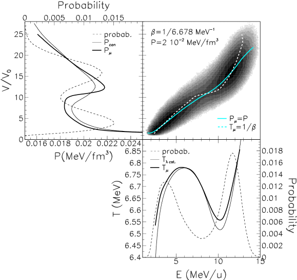
Figure 1: Right-upper panel: probability distribution (in log scale) of a canonical ensemble at constant pressure corresponding to the nucleus (200,82) where Coulomb interaction has been switched off. The canonical parameters $\beta$ and $P$ are labeled on the picture. The thick lines correspond to microcanonical isobaric and isothermal paths corresponding to $P_{\mu}=P$ and $T_{\mu}=1/\beta$. The lateral panels correspond to projections (dashed lines) of the probability distributions on $V/V_{0}$ (left) and $E$ (down) axes. Canonical pressure (left panel) and constant-$\lambda$ temperature are figured with thin lines. The corresponding microcanonical curves are plotted with thick lines. (Here and in the rest of the figures $E$ stands for excitation energy.)

While such constructions can be simply performed in theoretical models, experimentally one can usually only access microcanonical ensembles (due to the sorting of events in bins of $E$). Moreover, it is widely believed that the events corresponding to a microcanonical ensemble at a given $E$ have a fluctuating volume at freeze-out - somewhat similar to the case of a volume constraint $e^{-\lambda V}$ proposed in Ref. [2] (where $\lambda$ is the Lagrange multiplier corresponding to the volume observable). As clearly resulting from Fig. 1, the constant $\lambda$ microcanonical ensemble corresponds to the folding on the $V$ axis of the constant pressure canonical ensemble. Indeed, replacing in eq. (2) $\beta P$ with $\lambda$, and making the integration over $V$ one gets:

$${\mathcal{P}}^{\lambda}(E)=\frac{W^{\lambda}(E)~{}e^{-\beta E}}{Z_{can}(\beta,P)},$$ (5)

and then the expression of the microcanonical temperature:

$$T^{\lambda}_{\mu} = \left(\beta+\frac{\partial\ln{\mathcal{P}}^{\lambda}(E)}{\partial E}\right)^{-1}.$$ (6)

The dependence of the last two quantities on $E$ is represented in Fig. 1 (lower panel). Thus, ${\mathcal{P}}^{\lambda}(E)$ is a projection on the $E$ axis of the ${\mathcal{P}}(E,V)$ distribution. Therefore, a double peaked structure in ${\mathcal{P}}^{\lambda}(E)$ is necessarily related to a double peaked structure in ${\mathcal{P}}(E,V)$, and thus, is reflecting a first order liquid-gas phase transition as defined in Refs. [9, 8].

Of course, the same reasoning may be done for the projection on the $V$ axis. The corresponding curves are plotted in Fig. 1 (left panel). However, the relevance of this latter projection for the experimental data is conditioned by a good event by event resolution in freeze-out volume which was not achieved so far.

4 Microcanonical formulas

Let us further deduce the exact expressions for microcanonical temperature and heat capacity. The microcanonical density of states corresponding to a total energy of the system $E$ writes:

$$W(E)=\sum_{C^{\prime}}W_{C^{\prime}}$$ (7)

where

$$W_{C^{\prime}}=\frac{1}{N!}\left(\prod_{i=1}^{N}\frac{\rho_{i}(\epsilon_{i})}{h^{3}}\right)F({\mathcal{P}})f(n)\left[2\pi(E-{\mathcal{E}})\right]^{\frac{3}{2}(N-n)-1}$$ (8)

and

$$\sum_{C^{\prime}}()\equiv\sum_{N=1}^{A}\int\!\!\!\!\!\!\!\sum{\rm d}{\mathcal{E}}()\equiv\sum_{N=1}^{A}\prod_{i=1}^{N}\left(\sum_{A_{i},Z_{i}}\int{\rm d}{\bf r}_{i}\int{\rm d}\epsilon_{i}\right)()$$ (9)

Here $F({\mathcal{P}})$ is the factor in front of $f(n)$ from eq. (1) (${\mathcal{P}}$ is a generic notation for fragment partition) and ${\mathcal{E}}\equiv\sum_{i<j}V_{ij}+\sum_{i}\epsilon_{i}-\sum_{i}B_{i}$, the expression (9) being formal. Then, eq. (7) may be rewritten as:

$$W(E)=\sum_{N=1}^{A}\int\!\!\!\!\!\!\!\sum{\rm d}{\mathcal{E}}{\mathcal{F}}(C^{\prime})\left(E-{\mathcal{E}}\right)^{\frac{3}{2}(N-n)-1}.$$ (10)

The microcanonical temperature writes $T^{-1}=\partial S/\partial E$ with $S=\ln W(E)$. Which means:

$$T^{-1}=\frac{1}{W(E)}\frac{\partial W(E)}{\partial E}$$ (11)

If the limits of the (formal) integral over ${\mathcal{E}}$ are not depending on $E$, then one can simply make the derivative versus $E$ inside the integral from eq. (10):

$$T^{-1}=\frac{1}{W(E)}\sum_{C^{\prime}}W_{C^{\prime}}\left(\frac{\frac{3}{2}(N-n)-1}{E-{\mathcal{E}}}\right)=\left<\frac{\frac{3}{2}(N-n)-1}{K}\right>,$$ (12)

where we used the implication: $K=E-{\mathcal{E}}$ and the notation$\left<~{}\right>$ for the average over the ensemble’s states. The heat capacity of the system is by definition: $C^{-1}=-T^{2}\left(\partial^{2}S/\partial E^{2}\right)$. Using the same arguments as those from the deduction of $T$ one obtains:

$$C^{-1}=1-T^{2}\frac{1}{W(E)}\frac{\partial^{2}W(E)}{\partial E^{2}},$$ (13)

which implies:

$$C^{-1}=1-T^{2}\left<\frac{\left[\frac{3}{2}(N-n)-1\right]\left[\frac{3}{2}(N-n)-2\right]}{K^{2}}\right>.$$ (14)

Alternatively, one can (similarly) evaluate the second order derivative of the system’s entropy versus $E$:

$$\frac{\partial^{2}S}{\partial E^{2}}=\left<\frac{\left[\frac{3}{2}(N-n)-1\right]\left[\frac{3}{2}(N-n)-2\right]}{K^{2}}\right>-\left<\frac{\frac{3}{2}(N-n)-1}{K}\right>^{2}.$$ (15)

In these terms, the system’s spinodal region will be pointed by positive values of the above quantity. One can easily check that for $n=1$ (i.e. energy and total momentum are the conserved quantities), eq. (14) is similar with the one deduced in Ref. [6]. The microcanonical formulas given by eqs. (12), (14) and (15) are universally applicable to any system for which the “external” degrees of freedom can be treated classically irrespective to other specificities of the system. Indeed, the integral over the momenta variables (with the various possible conservation options) given in eq. (1), from which the microcanonical $T$, $C$ and $\partial^{2}S/\partial E^{2}$ formulas were further deduced is valid for any classical $N$ particle system. This is the case of nuclear multifragmentation as well: it is widely accepted that, since at freeze-out the system is rather dilute, a classical treatment of the fragments’ motion is appropriate. These features make eqs. (12), (14) and (15) suitable to be applied for experimental data: they are independent on specific model assumptions (i.e. freeze-out hypothesis, internal excitation treatment - level density, interfragment interactions, etc.), and moreover, they only depend on two parameters ($K$ and $N$) which have to be estimated for the freeze-out stage.

Figure 2: Comparison between the results of the microcanonical formulas (for temperature, heat capacity and second order derivative of the entropy) and the corresponding curves deduced from the probability distributions of a canonical ensemble with a given freeze-out constraint (i.e. constant volume or constant $\lambda$). Each column correspond to the case labeled on it.

5 Examples

While the deduction of the above formulas guarantees their accuracy, some examples of their functioning on concrete cases are further discussed. As an independent test, the results will be compared with the temperature/heat capacity computed using the method synthesized by eq. (6). More exactly, the caloric test curves are computed using eq. (6) from the probability distributions of a canonical ensemble with a given freeze-out constraint and the heat capacity and $\partial^{2}S/\partial E^{2}$ curves are farther evaluated from the obtained caloric curves ($C=\partial E/\partial T$, $\partial^{2}S/\partial E^{2}=(-1/T^{2})\partial T/\partial E$). Calculations are performed with both versions of the model ((i) and (ii)), for two different freeze-out constraints: constant $\lambda$ and constant volume, for the case in which the Coulomb interaction is present and the one in which it is switched off. (This variety of examples constitute a further test for the universality of the deduced formulas.) The considered conservation “level” is $n=2$, i.e. the total energy, the momentum and the angular momentum are conserved quantities. Results corresponding to the cases: (50,23) nucleus with constant $\lambda=5~{}10^{-4}$ fm^-3 with Coulomb interaction included, version (ii) of the model, (200,82), $\lambda=3~{}10^{-3}$ fm^-3, without Coulomb interaction, version (ii) of the model and the same nucleus with Coulomb interaction included, but a constant volume constraint: $V=10~{}V_{0}$, version (i) of the model are presented in Fig. 2 (first, middle and third column respectively). In the first two cases, backbendings of the caloric curves reflected in negative branches of the heat capacity curves and positive regions in the second order derivative of the entropy versus $E$ - all related with a first order phase transition can be observed. In the third case (constant volume constraint) the caloric curve has a monotonic increase with a “plateau-like” region (where the curve slope is smaller, but positive) which is reflected in a positive $C$ (with a peak in the plateau-like region) and a negative $\partial^{2}S/\partial E^{2}$. (As will be further seen, one cannot draw any conclusion from the third case concerning the intersection of the coexistence region since a constant volume path is not necessarily the order parameter of the system.) A very good agreement between the curves calculated using the probability distribution of a canonical ensemble and the points evaluated by means of the microcanonical formulas is to be noticed. The calculated microcanonical heat capacity and second derivative of the entropy versus excitation energy points are clearly revealing the spinodal region. While the calculated heat capacity points have large error bars near the border of the spinodal region due to the asymptotic behavior of the heat capacity, $\partial^{2}S/\partial E^{2}$ has small error bars even in the border region - thus being an even more robust quantity for identifying the spinodal region.

Figure 3: Kinetic energy distribution corresponding to the source nucleus (200,82) with the freeze-out volume $V=10~{}V_{0}$ with the Coulomb interaction included, for three excitation energies (0.5, 1 and 2 MeV/u).

Some details concerning the applicability of the microcanonical formulas have to mentioned. As mentioned earlier, the validity of these formulas is restricted by the condition that the integration domains in eq. (10) over the quantity ${\mathcal{E}}$ not to be restricted by the total energy of the system $E$. One should thus limit the cases on which this formula is applied to those obeying the above condition. But how to distinguish those “forbidden” points from the rest? A restriction by $E$ of the upper limit of the integral over ${\mathcal{E}}$ has to be clearly pointed by a “cut” in the right part of ${\mathcal{E}}$ distribution. Since $K=E-{\mathcal{E}}$, a similar “cut” (corresponding to $K=0$) has to be noticed in the left part of the $K$ probability distribution. In other words, when the probability that $K=0$ is significant (i.e. a cut clearly affects the $K$ distribution) then deviations from the microcanonical formulas should occur. These “cuts” (usually) occur at very low energies, so in a region unimportant for the system’s thermodynamics. All the points represented in Fig. 2 have been checked against the cut in the $K$ probability distribution. For illustrating this idea we take the case (200,82), with Coulomb, $V=10~{}V_{0}$. The probability distributions of $K$ corresponding to the $E=$0.5, 1 and 2 MeV/u cases are illustrated in Fig. 3. While the $K$ probability distributions corresponding to $E=$0.5 and 1 MeV/u are intersecting the $K=0$ axis, (giving thus a non-negligible probability for $K=0$), the probability distribution corresponding to the $E=2$ MeV/u case is not intersecting the $K=0$ vertical axis. This fixes the lowest excitation energy limit for which the microcanonical formula works to some value between 1 and 2 MeV/u.

Figure 4: Caloric curves, heat capacity curves and second order derivative of the entropy curves evaluated with the microcanonical formulas for the case of the nucleus (200,82), without Coulomb interaction and a freeze-out constrain corresponding to a path in $\lambda$ given by: $\lambda(E)=\lambda_{\mu}(E,10~{}V_{0})$.

The crossing of the spinodal region by a (experimental) path in the (E,V) plane may not be reflected as a backbending in a caloric curve. However, if the volume constraint is of the $e^{-\lambda V}$ type the spinodal region is likely to be revealed by a negative branch in the heat capacity. This point was nicely argued in Ref. [2] and can be evidenced by means of the present microcanonical formulas as a further test for their abilities. To this aim, we chose $\lambda$ as the microcanonical “$\lambda$” parameter ($\lambda_{\mu}$) corresponding to a constant volume path ($V=10~{}V_{0}$) in the (E,V) plane. I.e.:

$$\lambda(E)=\lambda_{\mu}(E,10~{}V_{0}).$$ (16)

The microcanonical $\lambda$ can be simply obtained from eq. (4):

$$\lambda_{\mu}=\lambda+\frac{\partial\ln{\mathcal{P}}(E,V)}{\partial V}.$$ (17)

As illustrated in Fig. 4 this path appears to intersect the system’s spinodal region without inducing any backbending in the caloric curve for the case of the system (200,82) without Coulomb interaction, (ii) version of the model. Indeed, while the caloric curve has a monotonical increase, the corresponding heat capacity presents a negative branch and the second order derivative of the entropy a positive region. The negative region in the heat capacity and the positive region in the second order derivative of the entropy versus energy are evidencing a “spinodal line” of the system corresponding to the volume $V=10~{}V_{0}$ in the system’s phase diagram in $(E,V)$ representation. The limits $E$ of this region are approximately those delimited by the above mentioned signals.

6 Fewer fragments

Let’s now assume that experimentally only a (small) number $N_{1}$ ($<N$) of fragments corresponding to a given event are detected. Can one still get the desired thermodynamical information about the system? This question is addressed in the present section. Let us turn back to eq. (1). For the highest conservation level ($n=2$) we can write:

$$I_{p} = \int\prod_{i=1}^{N}{\rm d}{\bf p}_{i}~{}\delta\left(\sum_{i}\frac{p_{i}^{2}}{2m_{i}}-K\right)\delta\left(\sum_{i}{\bf p}_{i}\right)\delta\left(\sum_{i}{\bf r}_{i}\times{\bf p}_{i}\right)$$ (18)

$$= \int\prod_{i=N_{1}+1}^{N}{\rm d}{\bf p}_{i}\int\prod_{i=1}^{N_{1}}{\rm d}{\bf p}_{i}~{}\delta\left(\sum_{i=1}^{N_{1}}\frac{p_{i}^{2}}{2m_{i}}-K_{1}\right)\delta\left(\sum_{i=1}^{N_{1}}{\bf p}_{i}-{\bf P}_{1}\right)\delta\left(\sum_{i=1}^{N_{1}}{\bf r}_{i}\times{\bf p}_{i}-{\bf L}_{1}\right),$$

where $K_{1}=E-{\mathcal{E}}-\sum_{i=N_{1}+1}^{N}p_{i}^{2}/(2m_{i})$, ${\bf P}_{1}=-\sum_{i=N_{1}+1}^{N}{\bf p}_{i}=\sum_{i=1}^{N_{1}}{\bf p}_{i}$ and ${\bf L}_{1}=-\sum_{i=N_{1}+1}^{N}{\bf r}_{i}\times{\bf p}_{i}=\sum_{i=1}^{N_{1}}{\bf r}_{i}\times{\bf p}_{i}$. The integration over the momenta of the first $N_{1}$ fragments can be further performed:

$$I_{p} \propto \int\prod_{i=N_{1}+1}^{N}{\rm d}{\bf p}_{i}\left(K_{1}-\frac{{\bf P}_{1}^{2}}{2M_{1}}-\frac{1}{2}{\bf L_{1}}^{T}{\bf I}_{1}^{-1}{\bf L_{1}}\right)^{\frac{3}{2}(N-2)-1}$$ (19)

$$\times \theta\left(K_{1}-\frac{{\bf P}_{1}^{2}}{2M_{1}}-\frac{1}{2}{\bf L_{1}}^{T}{\bf I}_{1}^{-1}{\bf L_{1}}\right)$$

where ${\bf I}_{1}$ is the inertial tensor corresponding to the first $N_{1}$ fragments at freeze-out, $M_{1}\equiv\sum_{i=1}^{N_{1}}m_{i}$ and $\theta$ stands for the step function. One can further deduce the thermodynamical quantities obtained before similarly, starting from their statistical definitions. In the general case (i.e a generic “level” of conservation $n$) one obtains:

$$T^{-1}=\left[\frac{3}{2}(N_{1}-n)-1\right]\left<\frac{1}{K_{2}}\right>,$$ (20)

$$C^{-1}=1-T^{2}\left[\frac{3}{2}(N_{1}-n)-1\right]\left[\frac{3}{2}(N_{1}-n)-2\right]\left<\frac{1}{K_{2}^{2}}\right>,$$ (21)

$$\frac{\partial^{2}S}{\partial E^{2}}=\left[\frac{3}{2}(N_{1}-n)-1\right]\left[\frac{3}{2}(N_{1}-n)-2\right]\left<\frac{1}{K_{2}^{2}}\right>-\left[\frac{3}{2}(N_{1}-n)-1\right]^{2}\left<\frac{1}{K_{2}}\right>^{2},$$ (22)

where $K_{2}=K_{1}-{\mathcal{K}}(n)$ with ${\mathcal{K}}(0)=0$, ${\mathcal{K}}(1)={\bf P}_{1}^{2}/(2M_{1})$ and ${\mathcal{K}}(2)={\mathcal{K}}(1)+{\bf L_{1}}^{T}{\bf I}_{1}^{-1}{\bf L_{1}}/2$. Following the same argumentation as in section 4 one can deduce the criterion of validity of the above formulas: the probability distribution of $K_{2}$ must not intersect the $K_{2}=0$ vertical axis at a non-negligible value. The advantages of the above formulas are obvious: they only depend on one parameter ($K_{2}$) and, more importantly, they can be used for inferring information about the liquid-gas phase transition even when one has incomplete information about the fragmentation events (i.e. only $N_{1}$ fragments from the $N$ fragments of one fragmentation event are detected). For a given microcanonical formula, depending on the desired conservation level ($n$), the minimum allowed value of $N_{1}$ is fixed by the condition that the factors containing $N_{1}$ be positive. Thus, for example, when only the total energy, $E$, is conserved ($n=0$) one only needs one freeze-out fragment per event in order to obtain the correct microcanonical temperature!

7 Summary

In summary, the possibilities of obtaining information about a possible liquid-gas phase transition from experimental heavy ion collision data have been investigated. The connection between negative heat capacity (or positive $\partial S^{2}/\partial E^{2}$) obtained in a fluctuating volume ensemble and the liquid gas phase transition has been discussed. It was shown that a negative value of the heat capacity in a fluctuating volume (constant $\lambda$) ensemble is in connection with a first order phase transition as defined in Ref. [8]. Microcanonical formulas for temperature, heat capacity and second order derivative of the entropy versus energy have been rigorously deduced for various conservation options (conserved energy; conserved energy and momentum; conserved energy, momentum and angular momentum). These formulas were tested with an independent method for obtaining the above mentioned quantities which extracts the microcanonical information from the probability distributions of a canonical ensemble with a given freeze-out volume constraint. An excellent agreement between the two methods have been obtained for all the considered curves ($T(E)$, $C(E)$, $\partial^{2}S/\partial E^{2}(E)$) for various cases ((50,23), $\lambda=5~{}10^{-4}$ fm^-3 with Coulomb, (200,82), $\lambda=3~{}10^{-3}$ fm^-3, without Coulomb, (200,82), $V=10~{}V_{0}$ with Coulomb). In the first two cases, backbendings in the caloric curves reflected in negative branches of the heat capacity curves and positive regions in the $\partial^{2}S/\partial E^{2}(E)$ curves have been obtained reflecting the occurrence of a first order phase transition. In the third case no backbending in the caloric curve or negative region in the heat capacity curve was observed which however does not imply any conclusion about the occurrence of a first order phase transition simply because a constant volume path in the $(E,V)$ plane is not necessarily the system’s order parameter. Indeed, choosing for the nucleus (200,82) without Coulomb a dependence of $\lambda$ on $E$ corresponding to the microcanonical lambda with $V=10~{}V_{0}$ ($\lambda(E)=\lambda_{\mu}(E,10~{}V_{0})$) in an ensemble with fluctuating volume one gets a well defined negative branch in the heat capacity curve and a positive region of the second order derivative of the entropy in spite of a monotonically increasing caloric curve. The case of incomplete (experimental) information concerning the fragmentation event is further discussed. Microcanonical formulas corresponding to all conservation levels depending only on a given number of fragments (smaller then the total number of fragments from the given event) are deduced. While demanding some more kinematical information about the detected fragments (only for the $n>0$ cases) their utility is obvious. Thus, for example in the $n=0$ case one only needs the kinetic energy of one freeze-out fragment per event in order to deduce the correct microcanonical temperature. The resulted microcanonical formulas are model independent thus being applicable on experimental data. Moreover they do not depend on any unevaluated term (such as heat capacity of a partial energy or the level density parameters as is the case in Ref.[4]). Of course, the success of these formulas depends on the accuracy of backtracking the information about the primary fragments. Here the microcanonical formulas based on partial break-up information may be very effective since some particles (such as freeze-out neutrons) carry at the asymptotic stage the untouched information about the freeze-out.

The authors thank the Alexander von Humboldt Foundation for supporting this work.

References

- [1] G. Bertsch and P. J. Siemens, Phys. Lett. B 126, 9 (1983).
- [2] Ph. Chomaz, V. Duflot, F. Gulminelli, Phys. Rev. Lett. 85, 3587 (2000).
- [3] Ph. Chomaz and F. Gulminelli, Nucl. Phys. A647, 153 (1999).
- [4] M. D’Agostino et al., Phys. Lett. B 473, 219 (2000).
- [5] M. D’Agostino et al., Nucl. Phys. A, in press.
- [6] Al. H. Raduta and Ad. R. Raduta, Nucl. Phys. A647, 12 (1999).
- [7] Al. H. Raduta and Ad. R. Raduta, Phys. Rev. C 55, 1344 (1997).
- [8] Al. H. Raduta and Ad. R. Raduta, Phys. Rev. Lett. 87, 202701 (2001).
- [9] Ph. Chomaz, F. Gulminelli, V. Duflot, Phys. Rev. E 64, 046114, (2001).