Gamow-Teller strength and the spin–isospin coupling constants
of the Skyrme energy functional

Abstract

We investigate the effects of the spin-isospin channel of the Skyrme energy functional on predictions for Gamow-Teller distributions and superdeformed rotational bands. We use the generalized Skyrme interaction SkO’ to describe even-even ground states and then analyze the effects of time-odd spin-isospin couplings, first term by term and then together via linear regression. Some terms affect the strength and energy of the Gamow-Teller resonance in finite nuclei without altering the Landau parameter $g_{0}^{\prime}$ that to leading order determines spin-isospin properties of nuclear matter. Though the existing data are not sufficient to uniquely determine all the spin-isospin couplings, we are able to fit them locally. Altering these coupling constants does not change the quality with which the Skyrme functional describes rotational bands.

]

I Introduction

Effective interactions for self-consistent nuclear structure calculations are usually adjusted to reproduce ground-state properties in even-even nuclei [1]. These properties depend only on terms in the corresponding energy functional that are bilinear in time-reversal-even (or “time-even”) densities and currents [2]. But the functional also contains an equal number of terms bilinear in time-odd densities and currents (see [2, 3] and refs. quoted therein), and these terms are seldom independently adjusted to experimental data. (For the sake simplicity we refer below to terms in the functional as time-even or time-odd, even though strictly speaking we mean the densities and currents on which they depend.) The time odd terms can be important as soon as time-reversal symmetry (and with it Kramers degeneracy) is broken in the intrinsic frame of the nucleus. Such breaking obviously occurs for rotating nuclei, in which the current and spin-orbit time-odd channels (linked to time-even channels by the gauge symmetry) play an important role. Time-odd terms also interfere with pairing correlations in the masses of odd-$A$ and odd-odd nuclei [4, 5, 6] and contribute to single-particle energies [7, 8, 9] and magnetic moments [10]. Finally, the spin-isospin channel of the effective interaction determines distributions of the Gamow-Teller (GT) strength.

The latter are the focus of this paper. We explore the effects of time-odd couplings on GT resonance energies and strengths, with an eye toward fixing the spin-isospin part of the Skyrme interaction. As discussed in our previous study [11], there are many good reasons for looking at this channel first. For instance, a better description of the GT response should enable more reliable predictions for $\beta$-decay half-lives of very neutron-rich nuclei. Those predictions in turn may help us identify the astrophysical site of r-process nucleosynthesis, which produces about half of the heavy nuclei with $A>70$.

Our goal is an improved description of GT excitations in a fully self-consistent mean-field model. To this end, we treat excited states in the Quasiparticle Random Phase Approximation (QRPA), with the residual interaction taken from the second derivative of the energy functional with respect to the density matrix. This approach is equivalent to the small-amplitude limit of time-dependent Hartree-Fock-Bogoliubov (HFB) theory. We proceed by taking the time-odd coupling constants in the Skyrme energy functional to be free parameters that we can fit to GT distributions. We then check that the coupling constants so deduced do not spoil the description of superdeformed (SD) rotational bands.

Our formulation is nonrelativisitic. In relativistic mean-field theory (RMF) [12, 13], the time-odd channels, referred to as “nuclear magnetism,” are not independent from the time-even ones because they arise from the small components of the Dirac wave functions. For rotational states, the time-odd effects have been extensively tested and shown to be important for reproducing experimental data (see, e.g., Ref. [14]). Only the current terms and spin-orbit terms play a role there, however, and the time-odd spin and spin-isospin channels of the RMF have never been tested against experimental data.

This paper is structured as follows: In Section II we review properties of the Skyrme energy functional. Section III reviews existing parameterizations of the functional, with particular emphasis on time-odd terms. Our main results are in Section IV, where we present calculations of GT strength and discuss the role played by the time-odd coupling constants. Section V describes calculations of moments of inertia for selected SD bands. Section VI contains our conclusions. We supplement our results with six Appendices that provide more detailed information on local densities and currents (Appendix A), early parameterizations of time-odd Skyrme functionals (Appendix B), the limit of the infinite nuclear matter (Appendix C), Landau parameters of Skyrme functionals (Appendix D) and of the Gogny force (Appendix E), and the residual interaction in finite nuclei from Skyrme functionals (Appendix F).

II A generalized Skyrme energy functional

A Basics of energy density theory

Many calculations performed with the Skyrme interaction can be viewed as energy-density theory in the spirit of the Hohenberg-Kohn-Sham approach [15], originally introduced for many-electron systems. Nowadays, energy density theory is a standard tool in atomic, molecular, cluster, and solid-state physics [16], as well as in nuclear physics [17]. The starting point is an energy functional ${\cal E}$ of all local densities and currents $\rho$, $\tau$, $\tensor{J}$, s, T, and j that can be constructed from the most general single-particle density matrix

$$\hat{\rho}\equiv\rho(\textbf{r},\sigma,\tau;\textbf{r}^{\prime},\sigma^{\prime},\tau^{\prime})=\sum_{k}v_{k}^{2}\;\psi_{k}^{*}(\textbf{r}^{\prime},\sigma^{\prime},\tau^{\prime})\;\psi_{k}(\textbf{r},\sigma,\tau)$$ (1)

(see Appendix A for more details), where r, $\sigma$, and $t$ are the spatial, spin, and isospin coordinates of the wave function. The Hohenberg-Kohn-Sham approach maps the nuclear many-body problem for the “real” highly correlated many-body wave function on a system of independent particles in so-called Kohn-Sham orbitals $\psi_{k}$. The equations of motion for $\psi_{k}$ are derived from the variational principle

$$\delta{\cal E}=0\quad\Rightarrow\quad\hat{h}\,\psi_{k}(\textbf{r},\sigma,\tau)=\epsilon_{k}\,\psi_{k}(\textbf{r},\sigma,\tau)~{},$$ (2)

where the single-particle Hamiltonian $\hat{h}$ is the sum of the kinetic term $\hat{t}$ and the self-consistent potential $\Gamma$ that is calculated from the density matrix

$$\hat{h}=\frac{\delta{\cal E}}{\delta\hat{\rho}}=\hat{t}+\hat{\Gamma}[\hat{\rho}]\quad.$$ (3)

The existence theorem for the effective energy functional makes no statement about its structure. The theoretical challenge is to find an energy functional that incorporates all relevant physics with as few free parameters as possible. The density functional approach as used here is equivalent to the local density approximation to the nuclear $G$ matrix [18].

The energy functional investigated here in detail describes the particle-hole channel of the effective interaction only. For the treatment of pairing correlations, the energy functional has to be complemented by an effective particle-particle interaction that is constructed in a similar way from the pairing density matrix; see [19] for details. We use here the simplest functional proportional to the square of the local pair density with the coupling constants given in [11].

B The Skyrme energy functional

Within the local-density approximation, the energy functional is given by the spatial integral of the local energy density ${\cal H}(\textbf{r})$

$${\cal E}=\int\!d^{3}\mathchoice{{\hbox{\boldmath$\displaystyle r$}}}{{\hbox{\boldmath$\textstyle r$}}}{{\hbox{\boldmath$\scriptstyle r$}}}{{\hbox{\boldmath$\scriptscriptstyle r$}}}\;{\cal H}(\textbf{r})~{}.$$ (4)

The energy density is composed of the kinetic term ${\cal H}_{\rm kin}$, the Skyrme energy density ${\cal H}_{\rm Skyrme}$ that describes the effective strong interaction between the nucleons, and a term arising from the electromagnetic interaction ${\cal H}_{\rm em}$:

$${\cal H}={\cal H}_{\rm kin}+{\cal H}_{\rm Skyrme}+{\cal H}_{\rm em}~{}.$$ (5)

For the electromagnetic interaction, we take the standard Coulomb expression, including the Slater approximation for the exchange term. The energy functional discussed here contains all possible terms bilinear in local densities and currents and up to second order in the derivatives that are invariant under reflection, time-reversal, rotation, translation, and isospin rotation [20].

Time-reversal invariance requires the energy density to be bilinear in either time-even densities or time-odd densities, so the Skyrme energy density can be separated into a “time-even” part ${\cal H}^{\rm even}$ and a “time-odd” part ${\cal H}^{\rm odd}$:

$${\cal H}_{\rm Skyrme} = \sum_{t=0,1}\sum_{t_{3}=-t}^{t}\Big{(}{\cal H}_{tt_{3}}^{\rm even}+{\cal H}_{tt_{3}}^{\rm odd}\Big{)}~{}.$$ (6)

The sum runs over the isospin $t$ and its third component $t_{3}$. Only the $t_{3}=0$ component of the isovector $t=1$ terms contribute to nuclear ground states and the rotational bands discussed later, while the $t_{3}=\pm 1$ components contribute only to charge-exchange (e.g. GT) excitations. In the notation of Refs.  [3, 20], the time-even and time-odd Skyrme energy densities read

$${\cal H}_{tt_{3}}^{\rm even}\! = \!C_{t}^{\rho}\,\rho_{tt_{3}}^{2}+C_{t}^{\Delta\rho}\,\rho_{tt_{3}}\Delta\rho_{tt_{3}}+C_{t}^{\tau}\,\rho_{tt_{3}}\tau_{tt_{3}}$$ (7)

$$+ \!C_{t}^{\nabla J}\rho_{tt_{3}}\,\nabla\cdot\textbf{J}_{tt_{3}}+C_{t}^{J}\tensor{J}^{2}_{tt_{3}},$$ (8)

$${\cal H}_{tt_{3}}^{\rm odd}\! = \!C_{t}^{s}\,\textbf{s}^{2}_{tt_{3}}+C_{t}^{\Delta s}\,\textbf{s}_{tt_{3}}\cdot\Delta\textbf{s}_{tt_{3}}+C_{t}^{T}\,\textbf{s}_{tt_{3}}\cdot\textbf{T}_{tt_{3}}$$ (9)

$$+ \!C_{t}^{\nabla s}\,(\nabla\cdot\textbf{s}_{tt_{3}})^{2}+C_{t}^{j}\,\textbf{j}^{2}_{tt_{3}}+C_{t}^{\nabla j}\,\textbf{s}_{tt_{3}}\cdot\nabla\times\textbf{j}_{tt_{3}}.\!\!$$ (10)

Isospin invariance of the Skyrme interaction makes the coupling constants independent of the isospin $z$-projection. All coupling constants might be density dependent. Following the standard ansatz for the Skyrme interaction, we neglect such a possibility except in $C_{t}^{\rho}$ and $C_{t}^{s}$, for which we restrict the density dependence to the following form

$$C_{t}^{\rho}[\rho_{0}] = C_{1}^{\rho}[0]+\Big{(}C_{1}^{\rho}[\rho_{\rm nm}]-C_{1}^{\rho}[0]\Big{)}\left(\frac{\rho_{0}}{\rho_{\rm nm}}\right)^{\alpha}~{},$$ (11)

$$C_{t}^{s}[\rho_{0}] = C_{1}^{s}[0]+\Big{(}C_{1}^{s}[\rho_{\rm nm}]-C_{1}^{s}[0]\Big{)}\left(\frac{\rho_{0}}{\rho_{\rm nm}}\right)^{\xi}.$$ (12)

Here $\rho_{0}$ is the isoscalar scalar density, and $\rho_{\rm nm}$ is its value in saturated infinite nuclear matter. The exponent $\alpha$ that specifies the density dependence of $C_{t}^{\rho}[\rho_{0}]$ must be about 0.25 for the incompressibility coefficient $K_{\infty}$ to be correct[21, 22, 23, 24]. Although this fact does not restrict the analogous power in $C_{t}^{s}[\rho_{0}]$, Eq. (12), we keep $\xi$ equal to $\alpha$ for simplicity here. Usually we will consider energy functionals that are invariant under local gauge transformations [3], which generalize the Galilean invariance of the Skyrme interaction discussed in [2]. Gauge invariance links three pairs of time-even and time-odd terms in the energy functional:

$$C_{t}^{j} = -C_{t}^{\tau}\quad,\quad C_{t}^{J}=-C_{t}^{T}\quad,\quad C_{t}^{\nabla j}=+C_{t}^{\nabla J}~{},$$ (13)

These relations fix all orbital time-odd terms, leaving only time-odd terms corresponding to the spin-spin interaction with free coupling constants. Relations (13) lead to a simplified form of Eqs. (6)–(9),

$${\cal H}_{\rm Skyrme} = \sum_{t=0,1}\sum_{t_{3}=-t}^{t}\Big{[}C_{t}^{\rho}\,\rho_{tt_{3}}^{2}+C_{t}^{s}\,\textbf{s}^{2}_{tt_{3}}$$ (14)

$$+ C_{t}^{\Delta\rho}\,\rho_{tt_{3}}\Delta\rho_{tt_{3}}+C_{t}^{\Delta s}\,\textbf{s}_{tt_{3}}\cdot\Delta\textbf{s}_{tt_{3}}$$ (15)

$$+ C_{t}^{\tau}\,(\rho_{tt_{3}}\tau_{tt_{3}}-\textbf{j}^{2}_{tt_{3}})+C_{t}^{T}\,(\textbf{s}_{tt_{3}}\cdot\textbf{T}_{tt_{3}}-\tensor{J}^{2}_{tt_{3}})$$ (16)

$$+ C_{t}^{\nabla J}\,(\rho_{tt_{3}}\,\nabla\cdot\textbf{J}_{tt_{3}}+\textbf{s}_{tt_{3}}\cdot\nabla\times\textbf{j}_{tt_{3}})$$ (17)

$$+ C_{t}^{\nabla s}\,(\nabla\cdot\textbf{s}_{tt_{3}})^{2}\Big{]}\quad.$$ (18)

The time-even terms of the energy functional can be directly related to nuclear bulk properties such as $E/A$, the saturation density $\rho_{\rm n.m.}$, incompressibility, symmetry energy, surface and surface symmetry energy, and spin-orbit splittings. The remaining time-odd terms cannot.

We will set the coupling constant $C_{t}^{\nabla s}$ to 0. The term it multiplies comes from a local two-body tensor force considered in Skyrme’s original papers [25] and discussed by Stancu et al. [26], but omitted in all modern Skyrme parameterizations except the force SL1 introduced by Liu et al. [27], which has not been used since.

III Existing parameterizations

The coupling constants of the time-odd Skyrme energy functional are usually taken from the (antisymmetrized) expectation value of a Skyrme force [2]. When so obtained, the 16 coupling constants of the energy functional (14) are uniquely linked to the 10 parameters $t_{i}$, $x_{i}$, $W_{0}$, and $\alpha$ of the standard Skyrme force (see Appendix B and Eq. (B7)). Only a few parameterizations rigidly enforce these relations, however. Among them are the forces of Ref. [21] (e.g. Z_σ), SkP [19], the Skyrme forces of Tondeur [28], the recent parameterizations SLy5 and SLy7 [24], and SkX [29]. Most other parameterizations neglect the $\tensor{J}^{2}$ term obtained from the two-body Skyrme force, setting $C_{t}^{T}=0$. Some authors do this for practical reasons; the $\tensor{J}^{2}$ term is time-consuming to calculate, and its contribution to the total binding energy is rather small. Other authors (see, e.g., [30]) find that including it with a coupling dictated from the HF expectation value of the Skyrme force can lead to unphysical solutions and/or unreasonable spin-orbit splittings. For spherical shapes, the $\tensor{J}^{2}$ term contributes to the time-even energy density in the same way as the neglected tensor force. One might therefore argue that by including the tensor force one could counterbalance the unwanted $\tensor{J}^{2}$ term exactly [30]. This argument, however, applies neither to deformed shapes nor to time-odd fields. Moreover, neglecting this term often violates self-consistency on the QRPA level (see below).

Although one might disagree with the rationale for neglecting the $\tensor{J}^{2}$ terms, it is not easy to adjust the coupling constants $C_{t}^{T}$ to spectral data. Large values for $C_{t}^{T}$ can be ruled out because they spoil the previously obtained agreement for single-particle spectra, but there are broad regions of values where they influence the usual time-even observables too weakly to be uniquely determined [31]. Only once in the published literature has there been an attempt to do so [32].

All first-generation Skyrme interactions, e.g., SI, SII [33], and SIII [30], used a three-body delta force instead of a density-dependent two-body delta-force to obtain reasonable nuclear-matter properties. The three-body interactions led to $\alpha=1$ for $C_{t}^{\rho}$ in Eq. (11), but a different density dependence of the $C_{t}^{s}$. $\alpha=1$ is too large to get the incompressibility $K_{\infty}$ right, and causes a spin instability in infinite nuclear matter [34] and finite nuclei [35] (again only within a microscopic potential framework). Both problems are cured with smaller values of $\alpha$ (between $1/6$ and $1/3$ [23]) but the second-generation interactions that did so still had problems in the time-odd channels, giving a poor description of spin and spin-isospin excitations and prompting several attempts to describe finite nuclei with extended Skyrme interactions. Krewald et al. [36], Waroquier et al. [37], and Liu et al. [27], for example, introduced additional three-body momentum-dependent forces. Waroquier et al. added an admixture of the density-dependent two-body delta force and a three-body delta force, while Liu et al. considered a tensor force. But none of these interactions has been used subsequently.

Van Giai and Sagawa [38] developed the more durable parameterization SGII, which gave a reasonable description of GT resonance data known at the time and is still used today. The fit to ground state properties was made without the $\tensor{J}^{2}$ terms, however, even though they were used in the QRPA. Consequently, in such an approach, the QRPA does not correspond to the small-amplitude limit of time-dependent HFB.

All these attempts to improve the description of the time-odd channels impose severe restrictions on the coupling by linking them to the HF expectation value of a Skyrme force, leading to one difficulty or another. The authors of Refs. [18, 39] proceed differently, treating the Skyrme energy functional as the result of a local-density approximation. The interpretation of the Skyrme interaction as an energy-density functional, besides relaxing the restrictions on the time-odd couplings, endows the spin-orbit interaction with a more flexible isospin structure [40, 41, 42] than can be obtained from the standard Skyrme force [43]. Some of the parameterizations used here will take advantage of that freedom. But the authors of Ref. [39] include only time-odd terms that are determined by gauge invariance; the other couplings are tentatively set to zero ($C_{t}^{s}=C_{t}^{\Delta s}=0$). Such a procedure is reasonable when describing natural parity excitations within the (Q)RPA, but the neglected spin-spin terms are crucial for the unnatural parity states that we discuss.

In this study, we use the energy-functional approach (14) with fully independent time-even and time-odd coupling constants. Our hope is that this more general formulation will improve the description of the GT properties while leaving the good description of ground-state properties in even nuclei untouched.

IV Giant Gamow–Teller resonances

The repulsive interaction between proton particles and neutron holes in the $J^{\pi}=1^{+}$ (spin-isospin) channel gives rise to a giant charge-exchange resonance in all nuclei with excess neutrons. The centroid of the resonance (which typically has a width of 5-10 MeV) can be roughly parameterized by the simple formula $E_{\rm GT}-E_{\rm F}=26A^{-1/3}-18.5(N-Z)A^{-1}$, where $E_{\rm F}$ is the centroid of the Fermi resonance [44]. This formula, however, captures only average behavior; individual cases depend on single-particle structure, and in particular the spin-orbit splitting.

The ability to model GT resonances is crucial for predictions of nuclear $\beta$ decay. Just as the low-lying $E1$ strength is depleted by the giant dipole resonance, so the low-lying GT strength, responsible for $\beta$ decay, is affected by the GT resonance. Since one of our future goals is an improved calculation of $\beta$-decay rates in nuclei along the $r$-process path, it is important to develop a reliable description of the GT giant resonance.

A Residual interaction in finite nuclei

Non-self-consistent calculations often use the residual Landau-Migdal interaction in the spin-isospin channel:

$$v_{\rm res}(\textbf{r},\textbf{r}^{\prime})$$ (19)

$$= N_{0}\Big{[}g_{0}^{\prime}\,\delta(\textbf{r}-\textbf{r}^{\prime})+g_{1}^{\prime}\,\textbf{k}^{\prime}\cdot\delta(\textbf{r}-\textbf{r}^{\prime})\,\textbf{k}\Big{]}(\mathchoice{{\hbox{\boldmath$\displaystyle\sigma$}}}{{\hbox{\boldmath$\textstyle\sigma$}}}{{\hbox{\boldmath$\scriptstyle\sigma$}}}{{\hbox{\boldmath$\scriptscriptstyle\sigma$}}}\cdot\mathchoice{{\hbox{\boldmath$\displaystyle\sigma$}}}{{\hbox{\boldmath$\textstyle\sigma$}}}{{\hbox{\boldmath$\scriptstyle\sigma$}}}{{\hbox{\boldmath$\scriptscriptstyle\sigma$}}}^{\prime})\,(\mathchoice{{\hbox{\boldmath$\displaystyle\tau$}}}{{\hbox{\boldmath$\textstyle\tau$}}}{{\hbox{\boldmath$\scriptstyle\tau$}}}{{\hbox{\boldmath$\scriptscriptstyle\tau$}}}\cdot\mathchoice{{\hbox{\boldmath$\displaystyle\tau$}}}{{\hbox{\boldmath$\textstyle\tau$}}}{{\hbox{\boldmath$\scriptstyle\tau$}}}{{\hbox{\boldmath$\scriptscriptstyle\tau$}}}^{\prime})$$ (20)

where $N_{0}$ is a normalization factor [see Eq. (D16)] and k and $\textbf{k}^{\prime}$ are defined in Appendix B. In most applications, only the $s$-wave interaction with strength $g_{0}^{\prime}$ is used, and the matrix elements of the force are not antisymmetrized. The underlying single-particle spectra are usually taken from a parameterized potential, e.g., the Woods-Saxon potential. Typical values for $g_{0}^{\prime}$, obtained from fits to GT-resonance systematics, are $1.4\leq g_{0}^{\prime}\leq 1.6$ [45, 46, 47]. (See Ref. [48] for an early compilation of data.) Sometimes this approach is formulated in terms of the residual interaction between antisymmetrized states. The results are similar, e.g., $g_{0}^{\prime}=1.54$ in the double-$\beta$-decay calculations by Engel et al. [49]. More complicated residual interactions, like boson-exchange potentials, have been used as well; see, e.g., Refs. [50, 51, 52]. Borzov et al. use a renormalized one-pion exchange potential in connection with a $\ell=0$ Landau-Migdal interaction of type (19) [53].

A much simpler residual interaction in the GT channel is a separable (or “schematic”) interaction, $v_{\rm res}=\kappa_{\rm GT}\;(\mathchoice{{\hbox{\boldmath$\displaystyle\sigma$}}}{{\hbox{\boldmath$\textstyle\sigma$}}}{{\hbox{\boldmath$\scriptstyle\sigma$}}}{{\hbox{\boldmath$\scriptscriptstyle\sigma$}}}\cdot\mathchoice{{\hbox{\boldmath$\displaystyle\sigma$}}}{{\hbox{\boldmath$\textstyle\sigma$}}}{{\hbox{\boldmath$\scriptstyle\sigma$}}}{{\hbox{\boldmath$\scriptscriptstyle\sigma$}}}^{\prime})\;(\mathchoice{{\hbox{\boldmath$\displaystyle\tau$}}}{{\hbox{\boldmath$\textstyle\tau$}}}{{\hbox{\boldmath$\scriptstyle\tau$}}}{{\hbox{\boldmath$\scriptscriptstyle\tau$}}}\cdot\mathchoice{{\hbox{\boldmath$\displaystyle\tau$}}}{{\hbox{\boldmath$\textstyle\tau$}}}{{\hbox{\boldmath$\scriptstyle\tau$}}}{{\hbox{\boldmath$\scriptscriptstyle\tau$}}}^{\prime})$, where the strength $\kappa_{\rm GT}$ has to be a function of $A$. This interaction is widely used in global calculations of nuclear $\beta$-decay [54, 55]. Sarriguren et al. [56] use it for a description of the GT resonances in deformed nuclei with quasiparticle energies obtained from self-consistent HF+BCS calculations. They estimate $\kappa_{\rm GT}$ from the Landau parameters of their Skyrme interaction. (The same prescription is used in their calculations of $M1$ resonances [57].) But however useful this approach may be from a technical point of view, it is not self-consistent. Nor is it equivalent to using the original residual Skyrme interaction; see, e.g., the discussion in [46].

A truly self-consistent calculation, by contrast, should interpret the QRPA as the small-amplitude limit of time-dependent HFB theory. The Skyrme energy functional used in the HFB should then determine the residual interaction between unsymmetrized states in the QRPA:

$$v_{\rm res}=\frac{\delta^{2}{\cal E}}{\delta\rho(\textbf{r}_{1},\sigma_{1},\tau_{1};\textbf{r}_{2},\sigma_{2},\tau_{2})\,\delta\rho(\textbf{r}_{1}^{\prime},\sigma_{1}^{\prime},\tau_{1}^{\prime};\textbf{r}_{2}^{\prime},\sigma_{2}^{\prime},\tau_{2}^{\prime})}~{}.$$ (21)

The actual form of the residual interaction that contributes to the QRPA matrix elements of $1^{+}$ states is outlined in Appendix F.

TABLE I.: Landau parameters for various Skyrme interactions from relations (B7) and the Gogny forces D1 and D1s. Missing entries are zero by construction.

Force	$g_{0}$	$g_{1}$	$g_{2}$	$g_{0}^{\prime}$	$g_{1}^{\prime}$	$g_{2}^{\prime}$
SkM*	$0.33$			$0.94$
SGII	$0.62$			$0.93$
SkP	$-0.23$	$-0.18$		$0.06$	$0.97$
SkI3	$1.89$			$0.85$
SkI4	$1.77$			$0.88$
SLy4	$1.39$			$0.90$
SLy5	$1.14$	$0.24$		$-0.15$	$1.05$
SLy6	$1.41$			$0.90$
SLy7	$0.94$	$0.47$		$0.02$	$0.88$
SkO	$0.48$			$0.98$
SkO’	$-1.61$	$2.16$		$0.79$	$0.19$
SkX	$-0.63$	$0.18$		$0.51$	$0.53$
D1	$0.47$	$0.06$	$0.12$	$0.60$	$0.34$	$0.08$
D1s	$0.48$	$-0.19$	$0.25$	$0.62$	$0.62$	$-0.04$

B GT strength distributions from existing Skyrme interactions

Before exploring the time-odd degrees of freedom of the generalized Skyrme energy functional, we analyze the performance of existing parameterizations when relations (B7) are used. We examine the forces SkP [19], SGII [38], SLy4, SLy5 [24], SkO, and SkO’[58], which all provide a good description of ground-state properties but differ in details. SkP uses an effective mass $m^{*}/m=1$ and is designed to describe both the mean-field and pairing effects. All other forces have smaller effective masses, so that $m^{*}/m\approx 0.9$ (SkO$x$) or even $m^{*}/m\approx 0.7$ (SGII, SLy$x$). SGII represents an early attempt to get good GT response properties from a standard Skyrme force. SLy4 and SLy5 are attempts to reproduce properties of pure neutron matter together with those of normal nuclear ground states. SkO and SkO’ are recent fits that include data from exotic nuclei, with particular emphasis on isovector trends in neutron-rich Pb isotopes; they complement the spin-orbit interaction with an explicit isovector degree-of-freedom [42]. All other parameterizations use the standard prescription $C_{0}^{\nabla J}=3C_{1}^{\nabla J}$.

Residual interactions are often summarized by the Landau parameters that appear in Eq. (19). The parameters can be derived as the corresponding coupling constants when Eq. (21) is evaluated for infinite spin-saturated symmetric nuclear matter (see Appendix D). In the literature, the infinite nuclear matter (INM) properties of the Skyrme interactions are usually calculated from Eqs. (B7). For the generalized energy functional (14) discussed here, the time-even INM properties such as the saturation density, energy per particle, effective mass, incompressibility, symmetry coefficient, and the time-even Landau parameters $f_{i}$, $f_{i}^{\prime}$ are unchanged, but properties of polarized INM and expressions for the time-odd Landau parameters $g_{i}$ and $g_{i}^{\prime}$ are different. We derive them in Appendix D. Here we are most concerned with the Landau parameters in the spin and spin-isospin channels,

$$g_{0} = N_{0}\big{(}2C_{0}^{s}+2C_{0}^{T}\,\beta\,\rho_{0}^{2/3}\big{)},$$ (23)

$$g_{0}^{\prime} = N_{0}\big{(}2C_{1}^{s}+2C_{1}^{T}\,\beta\,\rho_{0}^{2/3}\big{)},$$ (24)

$$g_{1} = -2N_{0}\;C_{0}^{T}\,\beta\,\rho_{0}^{2/3},$$ (25)

$$g_{1}^{\prime} = -2N_{0}\;C_{1}^{T}\,\beta\,\rho_{0}^{2/3},$$ (26)

FIG. 1.: Summed GT strength in ²⁰⁸Pb calculated with several Skyrme interactions, each corresponding to the Landau parameters $g_{0}^{\prime}$ and $g_{1}^{\prime}$ as indicated. The experimental resonance energy, taken from Ref. [46], is indicated by an arrow.

FIG. 2.: Same as in Fig. 2 except for ¹²⁴Sn.

where $N_{0}$ is given by (D16) and $\beta=(3\pi^{2}/2)^{2/3}$. Values for some typical Skyrme interactions appear in Table I. Higher-order Landau parameters are zero for the Skyrme functional (14). Some of these values differ from those given elsewhere because, unlike other authors, we insist on exactly the same effective interaction in the HFB and QRPA. The coupling constants $C^{T}_{0}$ and $C^{T}_{1}$ are fixed by the gauge invariance of the energy functional, which means that $C^{T}_{1}=0$ for SGII, SLy4 and SkO, because the $\tensor{J}^{2}$ term was omitted in the corresponding mean-field fits. For these interactions $g_{1}^{\prime}=0$ and $g_{0}^{\prime}\approx 0.9$. For SkP and SLy5, and SLy7, $C_{1}^{T}$ is relatively large (see Table IV), leading to a large $g_{1}^{\prime}\approx 1.0$, but a cancellation between two terms makes $g_{0}^{\prime}\approx 0.0$.

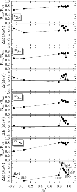
FIG. 3.: Deviation of the calculated GT resonance energy from experiment, $E_{\rm calc}-E_{\rm expt}$, and fraction of the GT strength in the resonance, $B_{\rm res}/B_{\rm tot}$, versus Landau parameter $g_{0}^{\prime}$, calculated for several Skyrme interactions (as indicated in the lower right panel) in ⁹⁰Zr, ¹¹²Sn, ¹²⁴Sn, and ²⁰⁸Pb. Experimental values are taken from Ref. [46].

Table I also gives values for the Landau parameters calculated for the Gogny forces D1 [59] and D1s [22] from the expressions provided in Appendix E. In the spirit of the Gogny force as a two-body potential, one has no freedom to choose the time-odd terms independently from the time-even ones. (Note that the Gogny force, however, employs the same local-density approximation for the density-dependence as the Skyrme energy functional that contributes to the $\ell=0$ Landau parameters.) The higher-order Landau parameters are uniquely fixed by the finite-range part of the Gogny force.

Figures 2 and 2 show the summed GT strength $B(GT)$ in ²⁰⁸Pb and ¹²⁴Sn, calculated with all the selected Skyrme forces. The ground-state energies are calculated as described in Ref. [11], and all strengths are divided by $1.26^{2}$, following common practice, to account for GT quenching. Although the GT resonance in ²⁰⁸Pb comes out at about the right energy for SGII, SLy4, SkO, and SkO’, it is too low for SkP and SLy5. These latter two interactions also leave too much GT strength at small excitation energies. It is tempting to interpret these findings in terms of the Landau parameters for these interactions. Schematic models suggest [1] that an increase of $g_{0}^{\prime}$ results in an increased resonance energy and more GT strength in the resonance. The nucleus ²⁰⁸Pb indeed behaves in this way, as can be seen in Fig. 2. The forces SkP and SLy5, with small values of $g_{0}^{\prime}$, yield more low-lying strength and a lower resonance energy than the remaining forces which correspond to $g_{0}^{\prime}\approx 0.9$.

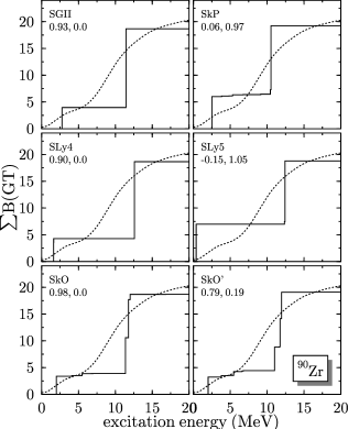
FIG. 4.: Same as in Fig. 2 except for ⁹⁰Zr. The very detailed experimental data are from a recent experiment by Wakasa et al. [60].

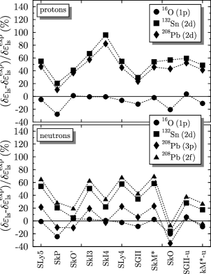
FIG. 5.: Relative errors in the spin-orbit splitting (calculated from the intrinsic single-particle energies) for the forces, nuclei, and states indicated. Only splittings between states which are both above or both below the Fermi surface are included. Other states are affected by core polarization and cannot be safely described by the mean field [7, 8]. The forces SLy5–SkO are ordered according to their values for $g_{0}^{\prime}$ (see Fig. 3). SGII–u and SkM^∗–u are two recent forces with modified spin-orbit interactions tailored for future use in GT resonance studies [62].

In ¹²⁴Sn, however, this simple picture does not hold, as Fig. 2 shows. The resonance energies are similar (and close to the experimental value) for SkP, SLy5, SkO, and SkO’ forces with very different values of $g_{0}^{\prime}$, while SGII and SLy4 push the resonance energy too high. Only the amount of the low-lying strength seems to scale with $g_{0}^{\prime}$. It is interesting, though, that the related forces SLy4 and SLy5 (which predict very similar single-particle spectra, but have quite different GT residual interactions) agree with the schematic model in that SLy4, with larger $g_{0}^{\prime}$, puts the GT resonance at a higher excitation energy.

It is clear that the scaling predicted by the schematic model is too simple, and Fig. 3 demonstrates this clearly. There we show the calculated strengths $B_{\rm res}$ in the GT resonances relative to the sum-rule value $B_{\rm tot}=3(N-Z)$, and the calculated GT resonance energies $E_{\rm calc}$ relative to the experimental values $E_{\rm expt}$. [For ⁹⁰Zr, ¹¹²Sn, ¹²⁴Sn, and ²⁰⁸Pb we used $E_{\rm expt}=9.4$ MeV, 8.9 MeV, 13.7 MeV, and 15.5 MeV, respectively [46]. Note that the calculated resonance energy depends on a prescription (see [11]) not strictly dictated by the QRPA.] The scatter near $g_{0}^{\prime}\approx 0.9$, in both the resonance energy and in the amount of low-lying strength, shows that other combinations of parameters in the residual interaction besides $g_{0}^{\prime}$ affect the GT distribution. This is not entirely surprising given the complexity of finite nuclei and of the interaction (21). In Sect. IV C we quantify these other important combinations and discuss their effects.

But another factor, this one determined by the time-even part of the Skyrme functional, affects the GT distribution: the underlying single-particle spectrum. Since GT transitions are especially sensitive to proton spin-orbit splittings, small changes in the time-even part of the force can, in principle, move the GT resonance considerably. Sensitivity to the spin-orbit splitting is particularly obvious in ⁹⁰Zr, where detailed information has been obtained from a recent experiment by Wakasa et al. [60]. Unlike in ¹²⁴Sn and ²⁰⁸Pb, which respond to a GT excitation in a collective way, the ⁹⁰Zr GT spectrum is dominated by two single-particle transitions, from the neutron $1g_{9/2}$ state to the proton $1g_{9/2}$ and $1g_{7/2}$ states. The difference between the locations of the two peaks in the GT spectrum is the sum of the proton $1g$ spin-orbit splitting and a contribution from the residual interaction (which can be expected to increase the difference). As Fig. 4 shows, all interactions, whatever their value for $g_{0}^{\prime}$, overestimate this difference; the resonance energy is always too large, even when the residual interaction is switched off completely.

Most Skyrme interactions give spin-orbit splittings in heavy nuclei that are too large [61]. We can therefore expect errors in their predicted GT strength distributions [45, 47]. Figure 5 shows errors in the predicted spin-orbit energies for the same forces as in Fig. 3. Interactions such as SkI3, SkI4, or SLy4 that overestimate the proton spin-orbit splittings give the largest resonance energies (and tend to overestimate them). The best interaction, in view of the combined information from Figs. 3 and 5, appears to be SkO’. Therefore, below, we use its time-even energy functional for further exploration of the time-odd terms.

We have included some new forces in Fig. 5; in a recent paper [62], Sagawa et al. attempt to improve the spin-orbit interaction for the standard Skyrme forces SIII, SkM^∗, and SGII, aiming at better GT-response predictions. They generalize the spin-orbit interaction through the condition $C_{0}^{\nabla J}=-C_{1}^{\nabla J}$ and include the $\tensor{J}^{2}$ term with a coupling given by Eq. (B7). Although the modified forces SkM^∗-u, and SGII-u give slightly better descriptions of GT resonances than the original interactions, they generate unacceptable errors in total binding energies and do not substantially improve the overall description of single-particle spectra in ²⁰⁸Pb.

A few remarks are in order before proceeding: (i) The spin-orbit splittings shown in Fig. 5 are calculated from intrinsic single-particle energies. Since experimental data are obtained from binding-energy differences between even-even and adjacent odd-mass nuclei, core polarization induced by the unpaired nucleon, which depends partly on time-odd channels of the interaction [7, 8], alters single-particle energies. The effect is largest in small nuclei (of the order of $20\%$ in ¹⁶O), decreasing rapidly with mass number [8]. (ii) GT distributions are also affected by the particle-particle channel of the effective interaction, but mainly at low energies. The GT resonance is not materially altered [11], so we can safely neglect the particle-particle interaction here.

C GT resonances from generalized Skyrme functionals

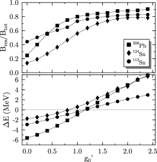
FIG. 6.: Deviation of calculated and experimental GT resonance energies (lower panel) and a fraction of the GT strength in the GT resonance (upper panel) for ¹¹²Sn, ¹²⁴Sn, and ²⁰⁸Pb, calculated with SkO’ and a modified residual spin-isospin interaction. $C_{1}^{T}$ is kept at the Skyrme-force value and $C_{1}^{\Delta s}$ is set to zero. $C_{1}^{s}$ is chosen to be density-independent and varied to get $0\leq g_{0}^{\prime}\leq 2.4$. $g_{1}^{\prime}=0.19$ in all cases.

We turn now to generalized energy functionals in which the time-odd coupling constants $C_{t}^{s}$, $C_{t}^{\Delta s}$, and $C_{t}^{T}$ are treated as free parameters; that is, we no longer insist that the interaction correspond to a two-body Hamiltonian with matrix elements that should be antisymmetrized. As we showed in Sect. IV B, values of the Landau parameter $g_{0}^{\prime}$ alone are insufficient to link the properties of the GT resonance to the coupling constants of the energy density functional. In this section, using the time-even functional of SkO’, we study the dependence of the GT resonance on several other combinations of the coupling constants as well. Because the isoscalar time-odd terms do not affect the GT transitions, we focus here on the isovector coupling constants $C_{1}^{s}$, $C_{1}^{\Delta s}$, and $C_{1}^{T}$.

1 Study of $C_{1}^{s}[\rho_{\rm nm}]$.

We begin with the simplest case, assuming that (i) the functional is gauge invariant, (ii) all time-odd coupling constants are density-independent, and (iii) the spin-surface term can be neglected, i.e., $C_{1}^{\Delta s}=0$. The only remaining free parameter in the spin-isospin channel is $C_{1}^{s}$, which is directly related to the Landau parameters via Eqs. (24) and (26):

$$C_{1}^{s}=\frac{1}{2N_{0}}\,(g_{0}^{\prime}+g_{1}^{\prime}),$$ (27)

where $g_{1}^{\prime}$ is fixed by $C_{1}^{T}$ [also in Eq. (26)]. Figure 6 shows results for the GT resonance energy when $g_{0}^{\prime}$ is systematically varied from its SkO’ value by altering $C_{1}^{s}$. We have chosen only nuclei that can be expected to exhibit a collective response to GT excitations. Non-collective contributions may show up, however, when the coupling constants are changed. In ¹²⁴Sn, for example, a state below the resonance collects a lot of strength for small values of $g_{0}^{\prime}$. Only by increasing $g_{0}^{\prime}$ does one push that strength into the resonance. Similarly, in ¹¹²Sn a state about 5 MeV above the resonance increasingly collects strength as $g_{0}^{\prime}$ grows.

As the underlying single-particle spectra are the same for all the cases in Fig. 6, the differences are due entirely to the value of $g_{0}^{\prime}$. With increasing $g_{0}^{\prime}$, the resonance energy increases and more strength is pushed into the resonance. The increase of $E_{\rm res}$ is nearly linear, but the lines for different nuclei have different slopes. It is gratifying that the curves for $E_{\rm calc}-E_{\rm expt}$ all have a zero around the same point, $g_{0}^{\prime}\approx 1.2$. This value is much smaller than the empirical value $g_{0}^{\prime}\approx 1.8$ derived earlier [63, 51, 52] for at least two reasons: (i) the influence of the single-particle spectrum, and (ii) the inclusion in the residual interaction of a $p$-wave force characterized by $g_{1}^{\prime}$. The latter means that $g_{0}^{\prime}=0$ does not correspond to a vanishing interaction in the spin-isospin channel.

FIG. 7.: Spatial dependence of $C_{1}^{s}[\rho]$ for various values of $x$$\equiv$$C_{1}^{s}[0]$/$C_{1}^{s}[\rho_{\rm nm}]$, cf. Eq. (12), and $g_{0}^{\prime}$ fixed at 1.2. The value $x=1$ corresponds to no density dependence. For larger values of $x$, the residual interaction becomes more repulsive outside the nucleus than inside. When $x=0$, $C_{1}^{s}[\rho]$ vanishes at large distances, and for negative values of $x$, the residual interaction becomes attractive outside the nucleus. The density profile $\rho(r)$ used in this plot corresponds to ²⁰⁸Pb.

2 Study of $C_{1}^{s}[0]$.

Thus far we have chosen not to let $C_{1}^{s}$ depend on the density. Little is known about the empirical density dependence of the time-odd energy functional, and time-odd Landau parameters calculated from a “realistic” one-boson exchange potential in DBHF show only a very weak density dependence [64]. Because the kinetic spin term $C_{1}^{T}\textbf{s}_{1t_{3}}\cdot\textbf{T}_{1t_{3}}$, when evaluated in INM, also contributes to the density dependence of the Landau parameters, the density-dependence of that term must either be small or nearly canceled by other time-odd terms. In any event, in the following, we investigate what happens when $C_{1}^{s}$ depends on the (isoscalar) density in the “standard” way (12). All nuclei we look at have finite neutron excess, which means that the central density should be slightly smaller than $\rho_{\rm nm}$.

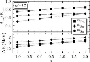
FIG. 8.: Variation of the GT resonance energy and the strength in the resonance when the ratio $x$$\equiv$$C_{1}^{s}[0]$/$C_{1}^{s}[\rho_{\rm nm}]$ of parameters defining the density dependence of $C_{1}^{s}[\rho]$ in Eq. (12) is varied. Symbols and scales are as in Fig. 6.

If $g_{0}^{\prime}$ and $g_{1}^{\prime}$ are fixed in saturated INM, there is one free parameter, $C_{1}^{s}[0]$, with which one can vary the density dependence (12). ($C_{1}^{s}[\rho_{\rm nm}]$ is fixed by the value $g_{0}^{\prime}[\rho_{\rm nm}]$=1.2, and we set the exponent $\xi$=0.25, as it is in the time-even energy functional SkO’.) We continue here to assume that gauge invariance holds, and that $C_{1}^{\Delta s}=0$.

We vary the parameter $C_{1}^{s}[0]$ between $-C_{1}^{s}[\rho_{\rm nm}]$ and $2C_{1}^{s}[\rho_{\rm nm}]$. Figure 7 shows the spatial dependence of $C_{1}^{s}[\rho]$ for several values of the ratio $x$$\equiv$$C_{1}^{s}[0]$/$C_{1}^{s}[\rho_{\rm nm}]$. By changing $C_{1}^{s}[0]$, one can change both the GT resonance energy and the amount of the low-lying strength, even with $g_{0}^{\prime}[\rho_{\rm nm}]$ kept constant. As Fig. 8 shows, an increase of $C_{1}^{s}[0]$ for a given $g_{0}^{\prime}$ has almost the same effect as an increase of $g_{0}^{\prime}$ for a given $C_{1}^{s}[0]$. Thus, the INM Landau parameters do not tell the whole story in a finite nucleus. Figures 7 and 8 show that the spin-spin coupling has the largest effect on the GT resonance when it is located at or even slightly outside the nuclear radius.

3 Study of $C_{1}^{\Delta s}$.

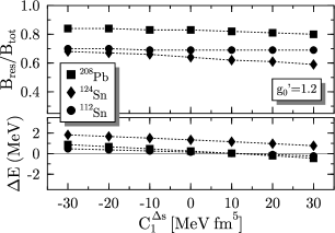
FIG. 9.: Variation of the GT resonance energy and the strength in the resonance when $C_{1}^{\Delta s}$ is varied. Symbols and scales are as in Fig. 6.

The term $C_{1}^{\Delta s}\textbf{s}_{1t_{3}}\cdot\Delta\textbf{s}_{1t_{3}}$ is sensitive to spatial variations of the isovector spin density. Unlike its (isoscalar) time-even counterpart $C_{0}^{\Delta\rho}\rho_{0}\Delta\rho_{0}$, it should not be called a “surface term” because the spatial distribution of $\textbf{s}_{1}$ is determined by a few single-particle states that do not necessarily vary the most at the nuclear surface. In discussing the effects of this term, we continue to fix $C_{1}^{T}$ at its Skyrme-force value via gauge invariance and choose $C_{1}^{s}$ to be density-independent and fixed from Eq. (27) with $g_{0}^{\prime}[\rho_{\rm nm}]=1.2$. We then vary $C_{1}^{\Delta s}$ over the range of $\pm 30\,{\rm MeV}\,{\rm fm}^{5}$, covering the values obtained from the original Skyrme forces. As seen in Fig. 9, an increase of $C_{1}^{\Delta s}$ by $30\,{\rm MeV}\,{\rm fm}^{5}$ has nearly the same effect on the GT resonance energies as a decrease of $g_{0}^{\prime}$ by 0.2, again demonstrating that the value of $g_{0}^{\prime}$ does not completely characterize the residual interaction in finite nuclei. A new feature of $C_{1}^{\Delta s}$, apparent from the curves for ¹¹²Sn and ²⁰⁸Pb in Fig. 9, is the ability to move the resonance around in energy without changing its strength.

4 Study of $C_{1}^{T}$.

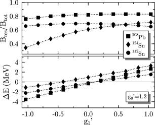
FIG. 10.: Variation of the GT resonance energy and the strength in the resonance when $C_{1}^{T}$ (and thus $g_{1}^{\prime}$) is varied. $C_{1}^{s}$ is readjusted for each value of $C_{1}^{T}$ so that $g_{0}^{\prime}=1.2$. Symbols and scales are as in Fig. 6.

Finally, we investigate the influence on the GT strength distribution of the term $C_{1}^{T}\textbf{s}_{1t_{3}}\cdot\textbf{T}_{1t_{3}}$, which determines $g_{1}^{\prime}$ [see Eq. (26)]. As this term is linked by gauge invariance (13) to the time-even $\tensor{J}^{2}_{1}$ term, a fully self-consistent variation of $C_{1}^{T}$ would require refitting the whole time-even sector of the Skyrme functional. (Note that our approach removes the constraints (B7) that link $C_{t}^{T}$ to the time-even coupling constants $C_{t}^{\tau}$ and $C_{t}^{\Delta\rho}$. The constraint was retained, however, when Sk0’ was constructed.) We leave that task for the future, using a gauge-invariance breaking-energy functional here with $C_{1}^{T}\neq C_{1}^{J}$ to obtain constraints on $C_{1}^{T}$ for future fits. Figure 10 shows the change in the GT resonance when $g_{1}^{\prime}$ is varied in the range $-1\leq g_{1}^{\prime}\leq 1$. Increasing $g_{1}^{\prime}$ increases the energy of the GT resonance for a given $g_{0}^{\prime}$. Changing $g_{1}^{\prime}$ by 0.2 has nearly the same effect on the GT resonance energy as changing $g_{0}^{\prime}$ by 0.2. (This means that $g_{0}^{\prime}=1.2$, $g_{1}^{\prime}=0.2$, as used here, is consistent with the lower end of the values $1.4\leq g_{0}^{\prime}\leq 1.6$, $g_{1}^{\prime}=0.0$ given in [45, 46, 47, 48].) As the curves for ²⁰⁸Pb and ¹¹²Sn demonstrate, however, the amount of strength in the resonance does not necessarily change when $g_{1}^{\prime}$ is varied.

D Regression analysis of the GT resonances

In the previous subsection we explored the dependence of the GT resonance energies and strengths on particular time-odd coupling constants of the Skyrme functional while keeping the other coupling constants fixed. These results show that the GT properties depend on all the coupling constants simultaneously, and the effect of varying one coupling constant may be either enhanced or cancelled by a variation of another one. In such a situation, linear-regression is needed to quantify the influence of the coupling constants.

We analyze the situation by supposing that the GT energies and strengths are linear functions of four coupling constants, i.e.,

$$E^{\rm GT}_{\rm reg}\! = e_{0}+e_{1}C_{1}^{s}[0]+e_{2}C_{1}^{s}[\rho_{\rm nm}]+e_{3}C_{1}^{\Delta s}+e_{4}C_{1}^{T},\!\!\!$$ (29)

$$B^{\rm GT}_{\rm reg}\! = b_{0}+b_{1}C_{1}^{s}[0]+b_{2}C_{1}^{s}[\rho_{\rm nm}]+b_{3}C_{1}^{\Delta s}+b_{4}C_{1}^{T}.\!\!\!$$ (30)

In our linear regression method, the coefficients $e_{i}$ and $b_{i}$ are determined by a least-square fit of expressions (29) and (30) to the given sample of $N$ calculated QRPA results, $E^{\rm GT}_{\rm calc}(n)$ and $B^{\rm GT}_{\rm calc}(n)$, $n=1,\ldots,N$. The calculated $B^{\rm GT}_{\rm calc}(n)$ values have been quenched by the usual factor of 1.26².

The sample of QRPA calculations covers the physically interesting range of values for the coupling constants. We present here results from a sample defined by the hypercube

$$g_{0}^{\prime}= 0.6(0.2)1.8, \quad\mbox{7 values},$$ (32)

$$C_{1}^{s}[0]/C_{1}^{s}[\rho_{\rm nm}]= -1(1)2, \quad\mbox{4 values},$$ (33)

$$C_{1}^{\Delta s}= -40(20)40, \quad\mbox{5 values},$$ (34)

$$C_{1}^{T}= -40(10)0, \quad\mbox{5 values},$$ (35)

i.e., for the sample of $N=700$. We use $g_{0}^{\prime}$ instead of $C_{1}^{s}[0]$ for the regression analysis to avoid combinations of the coupling constants that leave $g_{0}^{\prime}$ too far from 1.2, the value advocated in Sect. IV C.

The left panels in Figs. 11 and 12 contain histograms of deviations

$$\delta E^{\rm GT}(n) = E^{\rm GT}_{\rm calc}(n)-E^{\rm GT}_{\rm reg},$$ (37)

$$\delta B^{\rm GT}(n) = B^{\rm GT}_{\rm calc}(n)-B^{\rm GT}_{\rm reg}$$ (38)

between the calculated and fitted energies and strengths in ¹¹²Sn, ¹²⁴Sn, and ²⁰⁸Pb. The widths of these distributions illustrate the degree to which the linear regression expressions (IV D) are able to describe the results of the QRPA calculations. One can see that the fit GT resonance energies are generally within about $\pm 1$ MeV of the calculated ones, and the fit strengths within about $\pm$6.

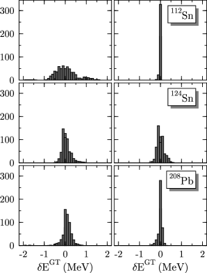
FIG. 11.: Distribution of differences between calculated GT resonance energies and those from the regression analysis, with all points from the sample (left panels) and with a reduced sample (right panels).

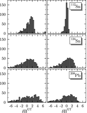
FIG. 12.: Same as in Fig. 11 except for the strength in the GT resonance.

As can be seen from Figs. 6, 8, 9, and 10, the dependence of both the resonance energy and the strength in the resonance on the coupling constants is not linear for the entire region of coupling constants. Although our sample is restricted to the area around the reasonable values, at times we leave the region where the regression can safely be performed. Furthermore, for certain combinations of the coupling constants (especially at a weak coupling), there are competing states that carry strength similar to that of the GT “resonance.” (These states often merge into the resonance at a larger coupling.) Finally, the resonance can be fragmented into many (sometimes up to 15) states. Therefore, we remove certain areas of parameter space where the determination of either the energy or the strength of the GT resonance is ambiguous. Such areas are almost always singled out by particularly large deviations from the fitted values.

	${}^{112}Sn$	${}^{124}Sn$	${}^{208}Pb$
$e_{0}$	$5.58100$	$10.16000$	$8.19600$
$e_{1}$	$0.00305$	$0.00488$	$0.00674$
$e_{2}$	$0.02696$	$0.03981$	$0.06099$
$e_{3}$	$0.01690$	$0.03474$	$0.05897$
$e_{4}$	$-0.01189$	$-0.01767$	$-0.02198$
$\sigma_{E}$	$0.0479$	$0.199$	$0.114$
$\sigma_{E}$(full)	$0.585$	$0.865$	$0.520$

TABLE II.: Coefficients $e_{i}$ obtained by the regression analysis, Eq. (29), of the QRPA GT resonance energies in the reduced sample (see text). The standard deviations $\sigma_{E}$ from this sample are compared to the $\sigma_{E}$(full) from the full sample of $N$=700 points.

	${}^{112}Sn$	${}^{124}Sn$	${}^{208}Pb$
$b_{0}$	$21.86000$	$11.75000$	$80.62000$
$b_{1}$	$0.00963$	$0.03107$	$0.03079$
$b_{2}$	$0.06143$	$0.25120$	$0.18620$
$b_{3}$	$0.09146$	$0.30510$	$0.33850$
$b_{4}$	$-0.01730$	$-0.10280$	$-0.09688$
$\sigma_{B}$	$0.608$	$2.10$	$2.74$
$\sigma_{B}$(full)	$5.20$	$3.44$	$3.82$

TABLE III.: Same as in Table II except for the strengths of the GT resonances.

After reducing the sample in this way, we obtain the histograms in the right panels of Figs. 11 and 12. These illustrate the quality of the regression fits obtained for samples of $N=542$, 664, and 618 in ¹¹²Sn, ¹²⁴Sn, and ²⁰⁸Pb, respectively. Tables II and III list the corresponding values of the regression coefficients, as well as the standard deviations for the GT energies and strengths within each of the samples.

Figures 11 and 12 and the standard deviations obtained in the reduced and full samples (Tables II and III) show that the description obtained by removing a small number of points beyond the region of linearity is quite good. The GT resonance energies are now reproduced within about $\pm$200 keV or less. The description of the resonant GT strengths is also improved, especially in ¹¹²Sn, although here the linear regression cannot work too well because the strengths saturate at strong coupling. Nevertheless, the coefficients listed in Tables II and III allow a fairly reliable estimate of the QRPA values for any combination of the coupling constants. The values of the coefficients in Tables II and III show that $C_{1}^{s}[\rho_{\rm nm}]$ and $C^{\Delta s}_{1}$ strongly influence properties of the GT resonance, and that both the energies and the resonant strengths increase when these coupling constants increase. $C^{T}_{1}$ has a weaker effect in the opposite direction, while $C^{s}_{1}[0]$ is less important still.

Without presenting detailed results, we report here on two other attempts at regression analysis. We tried to analyze the results for all the three nuclei, ¹¹²Sn, ¹²⁴Sn, and ²⁰⁸Pb, simultaneously by adding terms $e_{5}(N-Z)$ and $b_{5}(N-Z)$ to the regression formulas (IV D). Linear scaling might be obtained by analyzing the QRPA results for very many nuclei, where the effects due to shell structure could average out. In our small sample, shell structure is obviously important. We also tried the regression analysis with $C^{T}_{1}=-9.172$ MeV fm⁵ fixed at its SkO’ value (see Table IV), and without the terms $e_{4}$ and $b_{4}$ in the regression formulae (IV D), so that the functional’s gauge invariance was preserved. The results were not significantly different from those when $C^{T}_{1}$ was allowed to vary freely. Consequently, our analysis does not allow us any constraints on $C^{T}_{1}$ that might be used in future fits of the time-even part of the energy functional.

For the SkO’ coupling constants (see Table IV), we obtain $E^{\rm GT}_{\rm reg}=8.3$ MeV, 14.2 MeV, and 14.2 MeV in ¹¹²Sn, ¹²⁴Sn, and ²⁰⁸Pb, and $B^{\rm GT}_{\rm reg}=100$ in ²⁰⁸Pb. These values are close to the corresponding experimental data: 8.9 MeV, 13.7 MeV, 15.5 MeV, from Ref.[46], and $\sim 3(N-Z)/1.26^{2}$. It is not possible, however, to find values of the four coupling constants that reproduce these four experimental data points exactly. The reason is that the matrix of corresponding regression coefficients is almost singular, resulting in absurdly large values of the coupling constants. Clearly a determination of the coupling constants from experiment would require more data. Although charge-exchange measurements have been made on many nuclei, we require spherical even-even nuclei that are not soft against vibrations. To fit the relevant coupling constants to data, we would need, at the minimum, the ability to treat deformed nuclei. Meanwhile, we can make a simple choice of time-odd coupling constants from the analysis in Fig. 6. The values

$$C_{1}^{s}[0] =C_{1}^{s}[\rho_{\rm nm}]= 120\,{\rm MeV}\,{\rm fm}^{3}$$ (39)

$$C_{1}^{\Delta s} \phantom{C_{1}^{s}[\rho_{\rm nm}]=}= 0$$ (40)

$$C_{1}^{T} \phantom{C_{1}^{s}[\rho_{\rm nm}]=}= -9.172\,{\rm MeV}\,{\rm fm}^{5}$$ (41)

(see Table IV) give $g_{0}^{\prime}=1.2$ and $g_{1}^{\prime}$ = 0.19, which are in accord with the data we discuss. But these values by no means constitute a fit and are not unique.

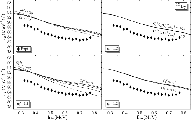
FIG. 13.: Dynamical moment of inertia ${\cal J}^{(2)}$ in the superdeformed band of ¹⁵²Dy calculated with the SkO’ energy density functional and modified time-odd coupling constants. In the upper left panel (corresponding to Fig. 6) all coupling constants are chosen to be density independent, $C_{1}^{\tau}$ is kept at the Skyrme-force value and $C_{1}^{\Delta s}=0$. In the upper right panel (corresponding to Fig. 8) the density dependence of $C_{1}^{s}$ is varied keeping $g_{0}^{\prime}=1.2$. In the lower left panel (corresponding to Fig. 9) $C_{1}^{\Delta s}$ is varied, while in the lower right panel (corresponding to Fig. 10) $C_{t}^{T}$ is varied. See text for the choice of isoscalar time-odd couplings.

V A consistency check: Superdeformed rotational bands

Another phenomenon in which the time-odd part of the Skyrme energy density functional plays a role is the high-spin rotation of very elongated nuclei. In this section we demonstrate that reasonable values for the spin-isospin coupling constants found when analyzing the GT strength are consistent with the description of superdeformed rotational bands.

When a nucleus rotates rapidly, there appear strong current and spin one-body densities along with the usual particle densities that characterize stationary (time-even) states. The time-odd densities are at the origin of strong time-odd mean fields. There are already many self-consistent studies of high-spin states available; see, e.g., reviews in Refs. [12, 65, 66, 67]. The role and significance of the time-odd mean-field terms, however, has not been carefully studied. Basic features of high-spin states can often be well described by models that use phenomenological mean fields of the Woods-Saxon or Nilsson type, where no time-odd terms are explicitly present in the one-body potential. (The time-odd densities are, however, present there through the time-odd cranking term.) For the Gogny interaction [59], or within the standard RMF models [12], they cannot be independently modified; the Gogny interaction is defined as a two-body force (where the time-odd terms show up as exchange terms), while all time-odd terms appearing in standard RMF models are fixed by Lorentz invariance. Within the Skyrme framework, the time-odd terms in superdeformed rotational states were analyzed in an exploratory way in Refs. [3, 20].

Unlike the GT response, rotational bands are influenced by both isoscalar and isovector time-odd channels of the effective interaction. In fact, the large effects of time-odd coupling constants found in [3] are mainly due to the isoscalar channel; the isovector channel induces corrections that are smaller, though non-negligible. The SkO’ Skyrme parameterization, which we use for GT calculations, is unstable when the original parameters from Eq. (B7) are used in the isoscalar spin channel because $g_{0}<-1$ (a fact that is related to the unusually high value of $g_{1}$ in Table I). This leads to unphysical ferromagnetic solutions where all spins align when the nucleus is cranked. Of course, the value of $g_{0}$ does not influence the GT calculations for even-even nuclei presented in our study which focuses on the isovector time-odd coupling constants. Consequently, in the following we employ a simple spin energy functional using the Skyrme force value for $C_{0}^{T}$, setting $C_{0}^{\Delta s}=0$ and neglecting density dependence. We adopt the value $g_{0}=0.4$ given in [52] (note that a different definition of the normalization factor is used there) to fix $C_{0}^{s}$.

We perform the calculations in exactly the same way as in Ref. [3] by using the code HFODD (v1.75r) described in Ref.[68]. We examine ¹⁵²Dy, which is a doubly magic superdeformed system. Pairing has a minor influence and we neglect it. We focus on the dynamic moment of inertia ${\cal J}_{2}$:

$${\cal J}^{(2)}(I)=\left[\frac{d^{2}E}{dI^{2}}\right]^{-1}\simeq\frac{4\hbar^{2}}{\Delta E_{\gamma}}$$ (42)

(from experimental data) or

$${\cal J}^{(2)}(\omega_{1})=\frac{dI}{d\omega}\simeq\frac{I(\omega_{1})-I(\omega_{2})}{\omega_{1}-\omega_{2}}$$ (43)

(in calculations). Figure 13 shows results of calculations when one of the four time-odd isovector coupling constants is varied, while the other ones are kept at the values mentioned above. Variations of the coupling constants $C_{1}^{s}[0]$, $C_{1}^{s}[\rho_{\rm nm}]$, and $C_{1}^{T}$ have little effect on the dynamic moments of inertia in ¹⁵²Dy. When $C_{1}^{\Delta s}$ is varied, the moments change noticeably, but the general trend with frequency is still the same. Thus, altering the isovector time-odd couplings does not appear to change the quality with which we describe superdeformed rotational bands. Of course, a consistent description of both the high-spin data and the GT resonance properties over a wide range of nuclei will require a much more detailed analysis.

VI Summary, conclusions, and outlook

By exploiting the freedom in the Skyrme energy functional, we have taken significant steps towards a fully self-consistent description of nuclear ground states and the GT response. Along the way, we debunked the notion that the strength and location of the GT resonance in finite nuclei is determined entirely by the Landau parameter $g_{0}^{\prime}$. Our analysis also shows this parameter to be smaller than previous work indicates.

There are not enough experimental data for spherical even-even nuclei to fix the time-odd isovector coupling constants; the ability to do calculations in deformed nuclei should help there. We could, however, choose values that reproduce the data we do analyze, without spoiling our description of high-spin superdeformation. Doing a lot better may require improving our time-even energy functionals. GT resonance energies and strengths depend significantly on spin-orbit splitting as well as the residual spin-isospin interaction. Until we are better able to reproduce single-particle energies, therefore, a fit of the time-odd interaction will be tentative.

We have not considered isoscalar time-odd interactions. The couplings there will be harder to fix because there are fewer data on the response, which is not as collective as in the charge-exchange channel. In addition, the isovector time-odd terms will play a role in calculations of isoscalar observables. Though a lot clearly remains to be done, our work can already be put to good use. We will, for example, employ the new values for the isovector time-odd coupling constants in future calculations of beta decay and in the observables that tell us about the extent of real time-reversal violation in nuclei.

A Local Densities and Currents

The complete density matrix $\rho(\textbf{r}\sigma t,\textbf{r}^{\prime}\sigma^{\prime}t^{\prime})$ in spin–isospin space as defined in (1) can be decomposed into the sum of scalar $\rho_{tt_{3}}(\textbf{r},\textbf{r}^{\prime})$ and vector densities $\textbf{s}_{tt_{3}}(\textbf{r},\textbf{r}^{\prime})$, where the subscripts denote the isospin quantum numbers:

$$\rho(\textbf{r}\sigma\tau,\textbf{r}^{\prime}\sigma^{\prime}\tau^{\prime})$$ (A1)

$$= {\textstyle\frac{{1}}{{4}}}\Big{[}\rho_{00}(\textbf{r},\textbf{r}^{\prime})\,\delta_{\sigma\sigma^{\prime}}\,\delta_{\tau\tau^{\prime}}+\textbf{s}_{00}(\textbf{r},\textbf{r}^{\prime})\cdot\mathchoice{{\hbox{\boldmath$\displaystyle\sigma$}}}{{\hbox{\boldmath$\textstyle\sigma$}}}{{\hbox{\boldmath$\scriptstyle\sigma$}}}{{\hbox{\boldmath$\scriptscriptstyle\sigma$}}}_{\sigma\sigma^{\prime}}\,\delta_{\tau\tau^{\prime}}$$ (A3)

$$+\delta_{\sigma\sigma^{\prime}}\!\sum_{t_{3}=-1}^{+1}\rho_{1t_{3}}(\textbf{r},\textbf{r}^{\prime})\tau^{t_{3}}_{\tau\tau^{\prime}}+\sum_{t_{3}=-1}^{+1}\textbf{s}_{1t_{3}}(\textbf{r},\textbf{r}^{\prime})\cdot\mathchoice{{\hbox{\boldmath$\displaystyle\sigma$}}}{{\hbox{\boldmath$\textstyle\sigma$}}}{{\hbox{\boldmath$\scriptstyle\sigma$}}}{{\hbox{\boldmath$\scriptscriptstyle\sigma$}}}_{\sigma\sigma^{\prime}}\tau^{t_{3}}_{\tau\tau^{\prime}}\Big{]}$$

The quantities $\mathchoice{{\hbox{\boldmath$\displaystyle\sigma$}}}{{\hbox{\boldmath$\textstyle\sigma$}}}{{\hbox{\boldmath$\scriptstyle\sigma$}}}{{\hbox{\boldmath$\scriptscriptstyle\sigma$}}}_{\sigma\sigma^{\prime}}$ and $\tau^{t_{3}}_{\tau\tau^{\prime}}$ are matrix elements of the Pauli matrices in spin and isospin space. In terms of these, the local density $\rho$, spin density s, kinetic density $\tau$, kinetic spin density T, current j, and spin-orbit tensor $\tensor{J}$ are

$$\rho_{tt_{3}}(\textbf{r}) = \rho_{tt_{3}}(\textbf{r},\textbf{r})\phantom{\Big{|}_{\textbf{r}=\textbf{r}^{\prime}}}$$ (A5)

$$\textbf{s}_{tt_{3}}(\textbf{r}) = \textbf{s}_{tt_{3}}(\textbf{r},\textbf{r})\phantom{\Big{|}_{\textbf{r}=\textbf{r}^{\prime}}}$$ (A6)

$$\tau_{tt_{3}}(\textbf{r}) = \nabla\cdot\nabla^{\prime}\rho_{tt_{3}}(\textbf{r},\textbf{r}^{\prime})\Big{|}_{\textbf{r}=\textbf{r}^{\prime}}$$ (A7)

$$\textbf{T}_{tt_{3}}(\textbf{r}) = \nabla\cdot\nabla^{\prime}\textbf{s}_{tt_{3}}(\textbf{r},\textbf{r}^{\prime})\Big{|}_{\textbf{r}=\textbf{r}^{\prime}}$$ (A8)

$$\textbf{j}_{tt_{3}}(\textbf{r}) = -{\textstyle\frac{{\text{i}}}{{2}}}(\nabla-\nabla^{\prime})\rho_{tt_{3}}(\textbf{r},\textbf{r}^{\prime})\Big{|}_{\textbf{r}=\textbf{r}^{\prime}}$$ (A9)

$$J_{tt_{3},ij}(\textbf{r}) = -{\textstyle\frac{{\text{i}}}{{2}}}(\nabla-\nabla^{\prime})_{i}\;s_{tt_{3},j}(\textbf{r},\textbf{r}^{\prime})\Big{|}_{\textbf{r}=\textbf{r}^{\prime}}\quad.$$ (A10)

The densities $\rho$, $\tau$, and $\tensor{J}$ are time-even, while s, T, and j are time-odd. See [20] for a more detailed discussion.

B Energy density functional from the two-body Skyrme force

TABLE IV.: Time-odd coupling constants calculated from Eq. (B7) for the Skyrme interactions as indicated.

Force	$C_{0}^{s}[0]$	$C_{1}^{s}[0]$	$C_{0}^{s}[\rho_{\rm nm}]$	$C_{1}^{s}[\rho_{\rm nm}]$	$C_{0}^{T}$	$C_{1}^{T}$	$C_{0}^{\Delta s}$	$C_{1}^{\Delta s}$	$\alpha$
	$({\rm MeV}\,{\rm fm}^{3})$	$({\rm MeV}\,{\rm fm}^{3})$	$({\rm MeV}\,{\rm fm}^{3})$	$({\rm MeV}\,{\rm fm}^{3})$	$({\rm MeV}\,{\rm fm}^{5})$	$({\rm MeV}\,{\rm fm}^{5})$	$({\rm MeV}\,{\rm fm}^{5})$	$({\rm MeV}\,{\rm fm}^{5})$
SkI1	$695.860$	$239.200$	$120.190$	$99.573$	$0.0$	$0.0$	$192.660$	$62.766$	$1/4$
SkI3	$84.486$	$220.360$	$253.180$	$113.940$	$0.0$	$0.0$	$92.235$	$22.777$	$1/4$
SkI4	$44.038$	$231.980$	$209.030$	$104.120$	$0.0$	$0.0$	$124.590$	$37.943$	$1/4$
SkO	$373.770$	$262.960$	$41.421$	$84.253$	$0.0$	$0.0$	$70.365$	$26.590$	$1/4$
SkO’	$277.910$	$262.430$	$47.082$	$84.154$	$-104.090$	$-9.172$	$42.791$	$16.553$	$1/4$
SkX	$57.812$	$180.660$	$-35.639$	$81.246$	$-7.861$	$-23.669$	$-4.434$	$9.514$	$1/2$
SGII	$271.110$	$330.620$	$61.048$	$91.676$	$0.0$	$0.0$	$15.291$	$15.283$	$1/6$
SkP	$152.340$	$366.460$	$-31.328$	$78.562$	$7.713$	$-41.127$	$-4.211$	$9.757$	$1/6$
SkM*	$271.110$	$330.620$	$31.674$	$91.187$	$0.0$	$0.0$	$17.109$	$17.109$	$1/6$
SLy4	$-207.820$	$311.110$	$153.210$	$99.737$	$0.0$	$0.0$	$47.048$	$14.282$	$1/6$
SLy5	$-171.360$	$310.430$	$151.080$	$99.133$	$-14.659$	$-65.058$	$45.787$	$14.000$	$1/6$
SLy6	$-201.460$	$309.940$	$157.050$	$100.280$	$0.0$	$0.0$	$48.822$	$14.655$	$1/6$
SLy7	$-215.830$	$310.100$	$158.260$	$100.640$	$-30.079$	$-55.951$	$49.680$	$14.843$	$1/6$

The standard two-body Skyrme force is given by [2, 33]

$$v_{\rm Skyrme}(\textbf{r}_{1},\textbf{r}_{2})$$ (B1)

$$= t_{0}\,(1+x_{0}\hat{P}_{\sigma})\;\delta(\textbf{r}_{1}-\textbf{r}_{2})$$ (B6)

$$+{\textstyle\frac{{1}}{{2}}}\;t_{1}\;(1+x_{1}\hat{P}_{\sigma})\Big{[}\hat{\textbf{k}}{}^{\prime 2}\;\delta(\textbf{r}^{\prime}_{1}-\textbf{r}^{\prime}_{2})+\delta(\textbf{r}_{1}-\textbf{r}_{2})\;\hat{\textbf{k}}{}^{2}\Big{]}$$

$$+t_{2}\,(1+x_{2}\hat{P}_{\sigma})\;\hat{\textbf{k}}{}^{\prime}\cdot\delta(\textbf{r}_{1}-\textbf{r}_{2})\;\hat{\textbf{k}}$$

$$+{\textstyle\frac{{1}}{{6}}}\,t_{3}\;(1+x_{3}\hat{P}_{\sigma})\;\delta(\textbf{r}_{1}-\textbf{r}_{2})\;\rho^{\alpha}\left({\textstyle\frac{{\textbf{r}_{1}+\textbf{r}_{2}}}{{2}}}\right)$$

$$+\text{i}W_{0}\,(\hat{\mathchoice{{\hbox{\boldmath$\displaystyle\sigma$}}}{{\hbox{\boldmath$\textstyle\sigma$}}}{{\hbox{\boldmath$\scriptstyle\sigma$}}}{{\hbox{\boldmath$\scriptscriptstyle\sigma$}}}}_{1}+\hat{\mathchoice{{\hbox{\boldmath$\displaystyle\sigma$}}}{{\hbox{\boldmath$\textstyle\sigma$}}}{{\hbox{\boldmath$\scriptstyle\sigma$}}}{{\hbox{\boldmath$\scriptscriptstyle\sigma$}}}}_{2})\cdot\hat{\textbf{k}}{}^{\prime}\times\delta(\textbf{r}_{1}-\textbf{r}_{2})\;\hat{\textbf{k}}\quad,$$

where $\hat{P}_{\sigma}={\textstyle\frac{{1}}{{2}}}(1+\hat{\mathchoice{{\hbox{\boldmath$\displaystyle\sigma$}}}{{\hbox{\boldmath$\textstyle\sigma$}}}{{\hbox{\boldmath$\scriptstyle\sigma$}}}{{\hbox{\boldmath$\scriptscriptstyle\sigma$}}}}_{1}\cdot\hat{\mathchoice{{\hbox{\boldmath$\displaystyle\sigma$}}}{{\hbox{\boldmath$\textstyle\sigma$}}}{{\hbox{\boldmath$\scriptstyle\sigma$}}}{{\hbox{\boldmath$\scriptscriptstyle\sigma$}}}}_{2}$) is the spin-exchange operator, $\hat{\textbf{k}}=-{\textstyle\frac{{\text{i}}}{{2}}}(\nabla_{1}-\nabla_{2})$ acts to the right, and $\hat{\textbf{k}}{}^{\prime}={\textstyle\frac{{\text{i}}}{{2}}}(\nabla_{1}^{\prime}-\nabla_{2}^{\prime})$ acts to the left. Calculating the Hartree-Fock expectation value from this force yields the energy functional given in Eq. (14) with the coupling constants:

$$C_{0}^{\rho} = {\textstyle\frac{{3}}{{8}}}t_{0}+{\textstyle\frac{{3}}{{48}}}t_{3}\,\rho_{0}^{\alpha}$$ (B7)

$$C_{1}^{\rho} = -{\textstyle\frac{{1}}{{4}}}t_{0}\Big{(}{\textstyle\frac{{1}}{{2}}}+x_{0}\Big{)}-{\textstyle\frac{{1}}{{24}}}t_{3}\Big{(}{\textstyle\frac{{1}}{{2}}}+x_{3}\Big{)}\,\rho_{0}^{\alpha}$$ (B8)

$$C_{0}^{s} = -{\textstyle\frac{{1}}{{4}}}t_{0}\Big{(}{\textstyle\frac{{1}}{{2}}}-x_{0}\Big{)}-{\textstyle\frac{{1}}{{24}}}t_{3}\Big{(}{\textstyle\frac{{1}}{{2}}}-x_{3}\Big{)}\,\rho_{0}^{\alpha}$$ (B9)

$$C_{1}^{s} = -{\textstyle\frac{{1}}{{8}}}t_{0}-{\textstyle\frac{{1}}{{48}}}t_{3}\,\rho_{0}^{\alpha}$$ (B10)

$$C_{0}^{\tau} = {\textstyle\frac{{3}}{{16}}}\,t_{1}+{\textstyle\frac{{1}}{{4}}}t_{2}\;\Big{(}{\textstyle\frac{{5}}{{4}}}+x_{2}\Big{)}$$ (B11)

$$C_{1}^{\tau} = -{\textstyle\frac{{1}}{{8}}}t_{1}\Big{(}{\textstyle\frac{{1}}{{2}}}+x_{1}\Big{)}+{\textstyle\frac{{1}}{{8}}}t_{2}\Big{(}{\textstyle\frac{{1}}{{2}}}+x_{2}\Big{)}$$ (B12)

$$C_{0}^{T} = \eta_{J}\,\Big{[}-{\textstyle\frac{{1}}{{8}}}t_{1}\Big{(}{\textstyle\frac{{1}}{{2}}}-x_{1}\Big{)}\,+{\textstyle\frac{{1}}{{8}}}t_{2}\Big{(}{\textstyle\frac{{1}}{{2}}}+x_{2}\Big{)}\Big{]}$$ (B13)

$$C_{1}^{T} = \eta_{J}\,\Big{[}-{\textstyle\frac{{1}}{{16}}}t_{1}+{\textstyle\frac{{1}}{{16}}}t_{2}\Big{]}$$ (B14)

$$C_{0}^{\Delta\rho} = -{\textstyle\frac{{9}}{{64}}}t_{1}+{\textstyle\frac{{1}}{{16}}}t_{2}\Big{(}{\textstyle\frac{{5}}{{4}}}+x_{2}\Big{)}$$ (B15)

$$C_{1}^{\Delta\rho} = {\textstyle\frac{{3}}{{32}}}t_{1}\Big{(}{\textstyle\frac{{1}}{{2}}}+x_{1}\Big{)}+{\textstyle\frac{{1}}{{32}}}t_{2}\Big{(}{\textstyle\frac{{1}}{{2}}}+x_{2}\Big{)}$$ (B16)

$$C_{0}^{\Delta s} = {\textstyle\frac{{3}}{{32}}}t_{1}\Big{(}{\textstyle\frac{{1}}{{2}}}-x_{1}\Big{)}+{\textstyle\frac{{1}}{{32}}}t_{2}\Big{(}{\textstyle\frac{{1}}{{2}}}+x_{2}\Big{)}$$ (B17)

$$C_{1}^{\Delta s} = {\textstyle\frac{{3}}{{64}}}t_{1}+{\textstyle\frac{{1}}{{64}}}t_{2}$$ (B18)

$$C_{0}^{\nabla J} = -{\textstyle\frac{{3}}{{4}}}W_{0}$$ (B19)

$$C_{1}^{\nabla J} = -{\textstyle\frac{{1}}{{4}}}W_{0}$$ (B20)

$$C_{0}^{\nabla s} = 0$$ (B21)

$$C_{1}^{\nabla s} = 0~{},$$ (B22)

nine of which are independent. Although in this approach $\eta_{J}=1$, many parameterizations of the Skyrme interaction set $\eta_{J}=0$. That violates the interpretation of the Skyrme functional as an expectation value of a real two-body interaction and removes the rationale for calculating the time-odd coupling constants from (B7). For Skyrme interactions with a generalized spin-orbit interaction [42], e.g. for SkI3, SkI4, SkO, or SkO’, the spin-orbit coupling constants are given by

$$C_{0}^{\nabla J}=-b_{4}-{\textstyle\frac{{1}}{{2}}}b_{4}^{\prime}\qquad,\qquad C_{1}^{\nabla J}=-{\textstyle\frac{{1}}{{2}}}b_{4}^{\prime}\quad.$$ (B23)

The resulting terms in the energy functional again cannot be represented as the HF expectation value of a two-body spin-orbit potential (see, e.g., [41]), again violating the assumptions behind the calculation of the time-odd coupling constants in (B7).

As Eqs. (B7) represent the standard approach to the time-odd coupling constants, it is worthwhile to take a look at the actual values. Table IV compares them for several Skyrme forces. None of these parameterizations was obtained from observables sensitive to the time-odd terms in the energy functional. Differences among the forces merely reflect various strategies for adjusting the time-even coupling constants. Values of the density-dependent isoscalar coupling constants $C_{0}^{s}$, either at $\rho_{0}=0$ or at $\rho_{0}=\rho_{\rm nm}$, are scattered in a wide range. This is probably one of the main sources of differences in the predictions of the forces for time-odd corrections to rotational bands. For the SLy$x$ forces, $C_{0}^{s}[0]$ is negative, which is unusual; most often this part of the isoscalar spin-spin interaction is repulsive at all densities. The difference will probably cause visible differences in rotational properties whenever the spin density is large at the surface. All the forces agree on the isovector coupling constant $C_{1}^{s}$, especially at the saturation density, i.e., $C_{1}^{s}[\rho_{\rm nm}]\approx 100\;$MeV fm³. This simply follows from the fact that, assuming Eq. (B7), $C_{1}^{s}$ is proportional to the time-even $C_{0}^{\rho}$ that is fixed from binding energies and radii.

C Infinite Nuclear Matter

1 Introduction

Homogeneous infinite nuclear matter (INM) is widely used to study and characterize nuclear interactions. Some INM properties, such as the saturation density, energy per particle, and asymmetry coefficient, are coherent, and others, such as the incompressibility $K_{\infty}$ and the sum-rule enhancement factor, are related to excitations and can be used as pseudo-observables to compare with predictions of nuclear forces. INM properties are also often used to adjust the parameters of effective interactions for self-consistent calculations. These properties at large asymmetry are key ingredients for the description of neutron stars. (See, e.g., Refs. [23, 69] for a discussion on the mean-field level.)

Most papers deal with spin-saturated INM, in which the time-odd channels of the interaction discussed here do not contribute. Nothing is known about spin-polarized INM, which actually may play some role in neutron stars. A stability criterion for this exotic system, derived in Ref. [70], was even used to adjust the parameters of the SLy$x$ forces in Ref.[23, 24]. We do not consider tensor forces in this work. Their contribution to the properties of polarized INM were explored, e.g., in Ref. [71].

2 Degrees of freedom

The four basic degrees of freedom of homogeneous INM are the isoscalar scalar density $\rho_{0}$, the isovector scalar density $\rho_{1}$, the isoscalar vector density $s_{0}$, and the isovector vector density $s_{1}$. They can be expressed through the usual neutron and proton, spin-up, and spin-down densities in the following way.

$$\rho_{0} = \rho_{{\rm n}\uparrow}+\rho_{{\rm n}\downarrow}+\rho_{{\rm p}\uparrow}+\rho_{{\rm p}\downarrow},$$ (C1)

$$\rho_{1} = \rho_{{\rm n}\uparrow}+\rho_{{\rm n}\downarrow}-\rho_{{\rm p}\uparrow}-\rho_{{\rm p}\downarrow},$$ (C2)

$$s_{0} = \rho_{{\rm n}\uparrow}-\rho_{{\rm n}\downarrow}+\rho_{{\rm p}\uparrow}-\rho_{{\rm p}\downarrow},$$ (C3)

$$s_{1} = \rho_{{\rm n}\uparrow}-\rho_{{\rm n}\downarrow}-\rho_{{\rm p}\uparrow}+\rho_{{\rm p}\downarrow}.$$ (C4)

Similarly, densities of protons and neutrons with spin up and down can be expressed as:

$$\rho_{{\rm n}\uparrow} = {\textstyle\frac{{1}}{{4}}}(\rho_{0}+\rho_{1}+s_{0}+s_{1})={\textstyle\frac{{1}}{{4}}}(1+I_{\tau}+I_{\sigma}+I_{\tau\sigma})\;\rho_{0},$$ (C5)

$$\rho_{{\rm n}\downarrow} = {\textstyle\frac{{1}}{{4}}}(\rho_{0}+\rho_{1}-s_{0}-s_{1})={\textstyle\frac{{1}}{{4}}}(1+I_{\tau}-I_{\sigma}-I_{\tau\sigma})\;\rho_{0},$$ (C6)

$$\rho_{{\rm p}\uparrow} = {\textstyle\frac{{1}}{{4}}}(\rho_{0}-\rho_{1}+s_{0}-s_{1})={\textstyle\frac{{1}}{{4}}}(1-I_{\tau}+I_{\sigma}-I_{\tau\sigma})\;\rho_{0},$$ (C7)

$$\rho_{{\rm p}\downarrow} = {\textstyle\frac{{1}}{{4}}}(\rho_{0}-\rho_{1}-s_{0}+s_{1})={\textstyle\frac{{1}}{{4}}}(1-I_{\tau}-I_{\sigma}+I_{\tau\sigma})\;\rho_{0},$$ (C8)

where $I_{\tau}=\rho_{1}/\rho_{0}$ is the relative isospin excess, $I_{\sigma}=s_{0}/\rho_{0}$ is the relative spin excess, and $I_{\sigma\tau}=s_{1}/\rho_{0}$ is the relative spin-isospin excess, with $-1\leq I_{i}\leq+1$.

In symmetric unpolarized INM $I_{i}=0$, while in asymmetric INM $\rho_{1}\neq 0$. Polarized INM has $s_{0}\neq 0$, and spin-isospin polarized nuclear matter has $s_{1}\neq 0$.

3 Fermi surfaces and kinetic densities

For INM arbitrary asymmetry, the Fermi energy of each particle species is different. Finite spin densities $s_{i}$ break the isotropy of INM, creating the possibility that the Fermi surface will deform[72]. We are mainly interested in INM with small polarization, so we use the approximation that all Fermi surfaces are spherical.

In the mean-field approximation, $\tilde{\rho}_{q\sigma}(\textbf{k})$, the density of particles in momentum space with the isospin projection $q$ and spin projection $\sigma$, is

$$\tilde{\rho}_{q\sigma}(\textbf{k})=\left\{\begin{array}[]{l}1\quad\mbox{for $k\leq k_{{\rm F},q\sigma}$},\\ 0\quad\mbox{for $k>k_{{\rm F},q\sigma}$}.\end{array}\right.$$ (C10)

In asymmetric polarized INM, the relation between the Fermi momenta and the isoscalar scalar density reads

$$\rho_{0}=\frac{2}{3\pi^{2}}\;k_{\rm F}^{3}=\frac{1}{6\pi^{2}}\sum_{q=p,n}\sum_{\sigma=\uparrow,\downarrow}k_{{\rm F},q\sigma}^{3}\quad,$$ (C11)

with $k_{{\rm F},q\sigma}=(6\pi^{2})^{1/3}\rho_{q\sigma}^{1/3}$. Here, $k_{\rm F}$ is the “average” Fermi momentum of the whole system. The kinetic density in momentum space for each particle species is given by

$$\tilde{\tau}_{q\sigma}(k)=k^{2}\,\tilde{\rho}_{q\sigma}(k),$$ (C12)

and the kinetic density in coordinate space is

$$\tau_{q\sigma}={\textstyle\frac{{V}}{{10\pi}}}k_{\rm F,q\sigma}^{5}={\textstyle\frac{{3}}{{20}}}\,\beta\,\rho_{q\sigma}^{5/3}\quad,$$ (C13)

where $\beta=(3\pi^{2}/2)^{2/3}$. Various kinetic densities in the spin-isospin space are given by

$$\tau_{0} = \tau_{{\rm n}\uparrow}+\tau_{{\rm n}\downarrow}+\tau_{{\rm p}\uparrow}+\tau_{{\rm p}\downarrow}={\textstyle\frac{{3}}{{5}}}\,\beta\,\rho_{0}^{5/3}F_{5/3}^{(0)}$$ (C14)

$$\tau_{1} = \tau_{{\rm n}\uparrow}+\tau_{{\rm n}\downarrow}-\tau_{{\rm p}\uparrow}-\tau_{{\rm p}\downarrow}={\textstyle\frac{{3}}{{5}}}\,\beta\,\rho_{0}^{5/3}F_{5/3}^{(\tau)}$$ (C15)

$$T_{0} = \tau_{{\rm n}\uparrow}-\tau_{{\rm n}\downarrow}+\tau_{{\rm p}\uparrow}-\tau_{{\rm p}\downarrow}={\textstyle\frac{{3}}{{5}}}\,\beta\,\rho_{0}^{5/3}F_{5/3}^{(\sigma)}$$ (C16)

$$T_{1} = \tau_{{\rm n}\uparrow}-\tau_{{\rm n}\downarrow}-\tau_{{\rm p}\uparrow}+\tau_{{\rm p}\downarrow}={\textstyle\frac{{3}}{{5}}}\,\beta\,\rho_{0}^{5/3}F_{5/3}^{(\sigma\tau)}~{},$$ (C17)

where $F_{m}^{(0)}$, $F_{m}^{(\tau)}$, $F_{m}^{(\sigma)}$, and $F_{m}^{(\sigma\tau)}$ are functions of the relative excesses:

$$F_{m}^{(0)} = {\textstyle\frac{{1}}{{4}}}\big{[}\big{(}1+I_{\tau}+I_{\sigma}+I_{\sigma\tau}\big{)}^{m}+\big{(}1+I_{\tau}-I_{\sigma}-I_{\sigma\tau}\big{)}^{m}$$ (C19)

$$+\big{(}1-I_{\tau}+I_{\sigma}-I_{\sigma\tau}\big{)}^{m}+\big{(}1-I_{\tau}-I_{\sigma}+I_{\sigma\tau}\big{)}^{m}\big{]}$$

This is a straightforward generalization of the corresponding definition for asymmetric unpolarized nuclear matter given in [23]. Similarly one defines

$$F_{m}^{(\tau)} = {\textstyle\frac{{1}}{{4}}}\big{[}\big{(}1+I_{\tau}+I_{\sigma}+I_{\sigma\tau}\big{)}^{m}+\big{(}1+I_{\tau}-I_{\sigma}-I_{\sigma\tau}\big{)}^{m}$$ (C22)

$$-\big{(}1-I_{\tau}+I_{\sigma}-I_{\sigma\tau}\big{)}^{m}-\big{(}1-I_{\tau}-I_{\sigma}+I_{\sigma\tau}\big{)}^{m}\big{]},$$

$$F_{m}^{(\sigma)} = {\textstyle\frac{{1}}{{4}}}\big{[}\big{(}1+I_{\tau}+I_{\sigma}+I_{\sigma\tau}\big{)}^{m}-\big{(}1+I_{\tau}-I_{\sigma}-I_{\sigma\tau}\big{)}^{m}$$ (C24)

$$+\big{(}1-I_{\tau}+I_{\sigma}-I_{\sigma\tau}\big{)}^{m}-\big{(}1-I_{\tau}-I_{\sigma}+I_{\sigma\tau}\big{)}^{m}\big{]},$$

$$F_{m}^{(\sigma\tau)} = {\textstyle\frac{{1}}{{4}}}\big{[}\big{(}1+I_{\tau}+I_{\sigma}+I_{\sigma\tau}\big{)}^{m}-\big{(}1+I_{\tau}-I_{\sigma}-I_{\sigma\tau}\big{)}^{m}$$ (C26)

$$-\big{(}1-I_{\tau}+I_{\sigma}-I_{\sigma\tau}\big{)}^{m}+\big{(}1-I_{\tau}-I_{\sigma}+I_{\sigma\tau}\big{)}^{m}\big{]}.$$

For calculations of INM properties, we also need derivatives of these functions. The first derivatives are given by

$$\frac{\partial F_{m}^{(\tau)}}{\partial I_{\tau}} = \frac{\partial F_{m}^{(\sigma)}}{\partial I_{\sigma}}=\frac{\partial F_{m}^{(\sigma\tau)}}{\partial I_{\sigma\tau}}=m\,F_{m-1}^{(0)},$$ (C28)

$$\frac{\partial F_{m}^{(0)}}{\partial I_{\tau}} = \frac{\partial F_{m}^{(\sigma)}}{\partial I_{\sigma\tau}}=\frac{\partial F_{m}^{(\sigma\tau)}}{\partial I_{\sigma}}=m\,F_{m-1}^{(\tau)},$$ (C29)

$$\frac{\partial F_{m}^{(0)}}{\partial I_{\sigma}} = \frac{\partial F_{m}^{(\tau)}}{\partial I_{\sigma\tau}}=\frac{\partial F_{m}^{(\sigma\tau)}}{\partial I_{\tau}}=m\,F_{m-1}^{(\sigma)},$$ (C30)

$$\frac{\partial F_{m}^{(0)}}{\partial I_{\sigma\tau}} = \frac{\partial F_{m}^{(\tau)}}{\partial I_{\sigma}}=\frac{\partial F_{m}^{(\sigma)}}{\partial I_{\tau}}=m\,F_{m-1}^{(\sigma\tau)},$$ (C31)

while the second derivatives are

$$\frac{\partial^{2}F_{m}^{(0)}}{\partial I_{i}^{2}} = m(m-1)\,F_{m-2}^{(0)},$$ (C32)

$$\frac{\partial^{2}F_{m}^{(j)}}{\partial I_{i}^{2}} = m(m-1)\,F_{m-2}^{(j)},$$ (C33)

for any $i,j=\tau,\sigma,\sigma\tau$. Functions of the order $m=0$ and $m=1$ are rather simple:

$$F_{0}^{(0)} = 1\quad,\quad F_{0}^{(i)}=0\quad,$$ (C34)

$$F_{1}^{(0)} = 1\quad,\quad F_{1}^{(i)}=I_{i}\quad,$$ (C35)

for any $i=\tau,\sigma,\sigma\tau$. Some special values $F_{m}^{(i)}(I_{\tau},I_{\sigma},I_{\sigma\tau})$ appearing in limiting cases of INM are

$$F_{m}^{(0)}(0,0,0) = 1\quad,\quad F_{m}^{(i)}(0,0,0)=0$$ (C36)

$$F_{m}^{(0)}(1,0,0) = F_{m}^{(0)}(0,1,0)=F_{m}^{(0)}(0,0,1)=2^{m-1}$$ (C37)

$$F_{m}^{(\tau)}(1,0,0) = F_{m}^{(\sigma)}(0,1,0)=F_{m}^{(\sigma\tau)}(0,0,1)=2^{m-1}$$ (C38)

$$F_{m}^{(0)}(1,1,1) = F_{m}^{(1)}(1,1,1)=4^{m-1}\quad.$$ (C39)

while $F_{m}^{(i)}=0$ if $I_{i}=0$ and one of the other $I_{j}$’s is equal to 1, with the last equal to zero. These functions are useful when writing down the equation of state and its derivatives.

4 “Equation of state” of asymmetric polarized nuclear matter

In INM $\Delta\rho_{tt_{3}}(\textbf{r})=\Delta\textbf{s}_{tt_{3}}(\textbf{r})(\textbf{r})=\textbf{j}_{tt_{3}}(\textbf{r})=\tensor{J}_{tt_{3}}(\textbf{r})=0$. We choose pure neutron and proton states, which leads to $\rho_{1,\pm 1}=0$, $\rho_{1}:=\rho_{1,0}$, and similarly for all other densities. We take the $z$ axis as the quantization axis for the spin, i.e., $s_{t,x}=s_{t,y}=0$, $s_{t}:=s_{t,z}$, and for the kinetic spin density T. As discussed in Refs. [72], this breaks the isotropy of INM, leading to an axially deformed Fermi surface, an effect which we neglect. Adding the kinetic term, the total energy per nucleon (i.e. the “equation of state”) for the energy functional (7) and (9) is given by

$$\frac{{\cal H}}{\rho_{0}} = {\textstyle\frac{{3}}{{5}}}{\textstyle\frac{{\hbar^{2}}}{{2m}}}\,\beta\,\rho_{0}^{2/3}\,F_{5/3}^{(0)}$$ (C43)

$$+\big{(}C_{0}^{\rho}+C_{1}^{\rho}\,I_{\tau}^{2}+C_{0}^{s}\,I_{\sigma}^{2}+C_{1}^{s}\,I_{\sigma\tau}^{2}\big{)}\,\rho_{0}$$

$$+{\textstyle\frac{{3}}{{5}}}\big{(}C_{0}^{\tau}F^{(0)}_{5/3}+C_{1}^{\tau}I_{\tau}F^{(\tau)}_{5/3}$$

$$+C_{0}^{T}I_{\sigma}F^{(\sigma)}_{5/3}+C_{1}^{T}I_{\sigma\tau}F^{(\sigma\tau)}_{5/3}\big{)}\,\beta\,\rho_{0}^{5/3}\,.$$

For unpolarized INM one has $I_{\sigma}=I_{\sigma\tau}=0$ which recovers the expression given in Ref.[23].

An interesting special case is polarized neutron matter, which is discussed in [70] for the Skyrme interactions. A stability criterion derived there from the two-body force point of view as outlined in Appendix B was used to constrain the parameters of the SLy$x$ forces [23, 24]. In this limiting case, one has $\rho_{{\rm n}\uparrow}=\rho_{0}$, $\rho_{{\rm n}\downarrow}=\rho_{{\rm p}\uparrow}=\rho_{{\rm p}\downarrow}=0$, which is equivalent to $I_{\tau}=I_{\sigma}=I_{\sigma\tau}=1$ and leads to

$$\frac{{\cal H}}{\rho_{0}} = 2^{4/3}\beta{\textstyle\frac{{3}}{{5}}}\left[{\textstyle\frac{{\hbar^{2}}}{{2m}}}+\big{(}C_{0}^{\tau}+C_{1}^{\tau}+C_{0}^{T}+C_{1}^{T}\big{)}\rho_{0}\right]\rho_{0}^{2/3}$$ (C45)

$$\quad+\big{(}C_{0}^{\rho}+C_{1}^{\rho}+C_{0}^{s}+C_{1}^{s}\big{)}\,\rho_{0}\quad.$$

Expressions (B7) for an antisymmetrized Skyrme force imply that $C_{0}^{\rho}+C_{1}^{\rho}+C_{0}^{s}+C_{1}^{s}=0$, and

$$\frac{{\cal H}}{\rho_{0}}=2^{4/3}\beta{\textstyle\frac{{3}}{{5}}}\left[{\textstyle\frac{{\hbar^{2}}}{{2m}}}+{\textstyle\frac{{1}}{{2}}}\,t_{2}\,(1+x_{2})\,\rho_{0}\right]\rho_{0}^{2/3}\quad.$$ (C46)

The stability of polarized neutron matter for all densities requires $x_{2}\approx-1$ [70], so the SLy$x$ interactions take $x_{2}\equiv-1$ [23, 24]. However, from the energy-density-functional point of view, the coupling constants are independent, and the second term in Eq. (C45) also contributes to the stability condition.

5 Pressure, Incompressibility and Asymmetry Coefficients

At the saturation point, all first derivatives of the energy per nucleon have to vanish and all second derivatives have to be positive. The first derivative with respect to $\rho_{0}$ is related to the pressure, the second derivative with respect to $\rho_{0}$ is related to the incompressibility, and the second derivatives with respect to the $I_{i}$ is related to the asymmetry coefficients. For symmetric matter, the first derivatives with respect to the $I_{i}$ vanish because the energy per nucleon is an even function of all $I_{i}$s. The pressure is given by

$$P=-\frac{\partial E}{\partial V}\bigg{|}_{A}=\rho_{0}^{2}\frac{\partial{\cal H}/\rho_{0}}{\partial\rho_{0}}\quad,$$ (C47)

which gives

$$P = {\textstyle\frac{{2}}{{5}}}{\textstyle\frac{{\hbar^{2}}}{{2m}}}\,\beta\,\rho_{0}^{5/3}F_{5/3}^{(0)}$$ (C52)

$$\quad+\big{(}C_{0}^{\rho}+C_{1}^{\rho}I_{\tau}^{2}+C_{0}^{s}I_{\sigma}^{2}+C_{1}^{s}I_{\sigma\tau}^{2}\big{)}\,\rho_{0}^{2}$$

$$\quad+3\rho_{0}^{2}\;\frac{\partial}{\partial\rho_{0}}\,\big{(}C_{0}^{\rho}+C_{1}^{\rho}I_{\tau}^{2}+C_{0}^{s}I_{\sigma}^{2}+C_{1}^{s}I_{\sigma\tau}^{2}\big{)}$$

$$\quad+\beta\Big{(}C_{0}^{\tau}\,F^{(0)}_{5/3}+C_{1}^{\tau}\,F^{(\tau)}_{5/3}\,I_{\tau}$$

$$\qquad+C_{0}^{T}\,F^{(\sigma)}_{5/3}\,I_{\sigma}+C_{1}^{T}\,F^{(\sigma\tau)}_{5/3}\,I_{\sigma\tau}\Big{)}\;\rho^{8/3}\quad.$$

The incompressibility is defined as

$$K=\frac{18P}{\rho_{0}}+9\rho_{0}^{2}\frac{\partial^{2}{\cal H}/\rho_{0}}{\partial\rho_{0}^{2}},$$ (C53)

which, for the Skyrme energy functional (C43) at the saturation point ($\rho_{0}=\rho_{\rm n.m.}$, $I_{\tau}=I_{\sigma}=I_{\sigma\tau}=0$) gives

$$K_{\infty} = -{\textstyle\frac{{6}}{{5}}}\left({\textstyle\frac{{\hbar^{2}}}{{2m}}}-5C_{0}^{\tau}\,\rho_{0}\right)\beta\,\rho_{0}^{2/3}F_{5/3}^{(0)}$$ (C55)

$$+2\rho_{0}^{2}\frac{\partial C_{0}^{\rho}}{\partial\rho_{0}}+\rho_{0}^{3}\frac{\partial^{2}C_{0}^{\rho}}{\partial^{2}\rho_{0}}.$$

The asymmetry coefficients are:

$$a_{\tau} = \frac{1}{2}\frac{\partial^{2}{\cal H}/\rho_{0}}{\partial I_{\tau}^{2}}\bigg{|}_{I_{\tau}=I_{\sigma}=I_{\sigma\tau}=0}$$ (C56)

$$= {\textstyle\frac{{1}}{{3}}}\left[{\textstyle\frac{{\hbar^{2}}}{{2m}}}+(C_{0}^{\tau}+3C_{1}^{\tau})\,\rho_{0}\right]\beta\,\rho_{0}^{2/3}+C_{1}^{\rho}\,\rho_{0},$$ (C57)

$$a_{\sigma} = \frac{1}{2}\frac{\partial^{2}{\cal H}/\rho_{0}}{\partial I_{\sigma}^{2}}\bigg{|}_{I_{\tau}=I_{\sigma}=I_{\sigma\tau}=0}$$ (C58)

$$= {\textstyle\frac{{1}}{{3}}}\left[{\textstyle\frac{{\hbar^{2}}}{{2m}}}+(C_{0}^{\tau}+3C_{0}^{T})\,\rho_{0}\right]\beta\,\rho_{0}^{2/3}+C_{0}^{s}\,\rho_{0},$$ (C59)

$$a_{\sigma\tau} = \frac{1}{2}\frac{\partial^{2}{\cal H}/\rho_{0}}{\partial I_{\sigma\tau}^{2}}\bigg{|}_{I_{\tau}=I_{\sigma}=I_{\sigma\tau}=0}$$ (C60)

$$= {\textstyle\frac{{1}}{{3}}}\left[{\textstyle\frac{{\hbar^{2}}}{{2m}}}+(C_{0}^{\tau}+3C_{1}^{T})\,\rho_{0}\right]\beta\,\rho_{0}^{2/3}+C_{1}^{s}\,\rho_{0}.$$ (C61)

Here, $a_{\tau}$ is the well-known volume asymmetry coefficient of the liquid-drop model, and $a_{\sigma}$ and $a_{\sigma\tau}$ are its generalizations to the spin and spin-isospin channels of the interaction. At the saturation point, all asymmetry coefficients have to be positive.

D Landau Parameters from the Skyrme energy functional

A simple and instructive description of the residual interaction in homogeneous INM is given by the Landau interaction developed in the context of Fermi-liquid theory [50]. Landau parameters corresponding to the Skyrme forces are discussed in Refs. [21, 27, 36, 37, 38, 73]. Starting from the full density matrix in (relative) momentum space $\tilde{\rho}(\textbf{k}\sigma\tau\sigma^{\prime}\tau^{\prime})$, the various densities are defined as

$$\tilde{\rho}_{00}(\textbf{k}) = \sum_{\sigma}\sum_{\tau}\tilde{\rho}(\textbf{k}\sigma\tau\sigma\tau),$$ (D2)

$$\tilde{\rho}_{1t_{3}}(\textbf{k}) = \sum_{\sigma}\sum_{\tau,\tau^{\prime}}\tilde{\rho}(\textbf{k}\sigma\tau\sigma\tau^{\prime})\;\tau^{t_{3}}_{\tau\tau^{\prime}},$$ (D3)

$$\tilde{\textbf{s}}_{00}(\textbf{k}) = \sum_{\sigma,\sigma^{\prime}}\sum_{\tau}\tilde{\rho}(\textbf{k}\sigma\tau\sigma^{\prime}\tau)\;\mathchoice{{\hbox{\boldmath$\displaystyle\sigma$}}}{{\hbox{\boldmath$\textstyle\sigma$}}}{{\hbox{\boldmath$\scriptstyle\sigma$}}}{{\hbox{\boldmath$\scriptscriptstyle\sigma$}}}_{\sigma\sigma^{\prime}},$$ (D4)

$$\tilde{\textbf{s}}_{1t_{3}}(\textbf{k}) = \sum_{\sigma,\sigma^{\prime}}\sum_{\tau,\tau^{\prime}}\tilde{\rho}(\textbf{k}\sigma\tau\sigma^{\prime}\tau^{\prime})\>\mathchoice{{\hbox{\boldmath$\displaystyle\sigma$}}}{{\hbox{\boldmath$\textstyle\sigma$}}}{{\hbox{\boldmath$\scriptstyle\sigma$}}}{{\hbox{\boldmath$\scriptscriptstyle\sigma$}}}_{\sigma\sigma^{\prime}}\;\tau^{t_{3}}_{\tau\tau^{\prime}},$$ (D5)

The kinetic densities are given by $\tau_{tt_{3}}=\rho_{tt_{3}}\,k^{2}$, $\textbf{T}_{tt_{3}}=\textbf{s}_{tt_{3}}\,k^{2}$. The Landau-Migdal interaction is defined as

$$\tilde{F}(\textbf{k}_{1}\sigma_{1}\tau_{1}\sigma^{\prime}_{1}\tau^{\prime}_{1};\textbf{k}_{2}\sigma_{2}\tau_{2}\sigma^{\prime}_{2}\tau^{\prime}_{2})$$ (D6)

$$= \frac{\delta^{2}{\cal E}}{\delta\tilde{\rho}(\textbf{k}_{1}\sigma_{1}\tau_{1}\sigma^{\prime}_{1}\tau^{\prime}_{1})\delta\tilde{\rho}(\textbf{k}_{2}\sigma_{2}\tau_{2}\sigma^{\prime}_{2}\tau^{\prime}_{2})}$$ (D7)

$$= \tilde{f}(\textbf{k}_{1},\textbf{k}_{2})+\tilde{f}{}^{\prime}(\textbf{k}_{1},\textbf{k}_{2})\;\mathchoice{{\hbox{\boldmath$\displaystyle\tau$}}}{{\hbox{\boldmath$\textstyle\tau$}}}{{\hbox{\boldmath$\scriptstyle\tau$}}}{{\hbox{\boldmath$\scriptscriptstyle\tau$}}}_{1}\cdot\mathchoice{{\hbox{\boldmath$\displaystyle\tau$}}}{{\hbox{\boldmath$\textstyle\tau$}}}{{\hbox{\boldmath$\scriptstyle\tau$}}}{{\hbox{\boldmath$\scriptscriptstyle\tau$}}}_{2}\phantom{\frac{\delta^{2}}{\tilde{\rho}}}$$ (D9)

$$+\tilde{g}(\textbf{k}_{1},\textbf{k}_{2})\;\mathchoice{{\hbox{\boldmath$\displaystyle\sigma$}}}{{\hbox{\boldmath$\textstyle\sigma$}}}{{\hbox{\boldmath$\scriptstyle\sigma$}}}{{\hbox{\boldmath$\scriptscriptstyle\sigma$}}}_{1}\cdot\mathchoice{{\hbox{\boldmath$\displaystyle\sigma$}}}{{\hbox{\boldmath$\textstyle\sigma$}}}{{\hbox{\boldmath$\scriptstyle\sigma$}}}{{\hbox{\boldmath$\scriptscriptstyle\sigma$}}}_{2}+\tilde{g}{}^{\prime}(\textbf{k}_{1},\textbf{k}_{2})\,(\mathchoice{{\hbox{\boldmath$\displaystyle\sigma$}}}{{\hbox{\boldmath$\textstyle\sigma$}}}{{\hbox{\boldmath$\scriptstyle\sigma$}}}{{\hbox{\boldmath$\scriptscriptstyle\sigma$}}}_{1}\cdot\mathchoice{{\hbox{\boldmath$\displaystyle\sigma$}}}{{\hbox{\boldmath$\textstyle\sigma$}}}{{\hbox{\boldmath$\scriptstyle\sigma$}}}{{\hbox{\boldmath$\scriptscriptstyle\sigma$}}}_{2})(\mathchoice{{\hbox{\boldmath$\displaystyle\tau$}}}{{\hbox{\boldmath$\textstyle\tau$}}}{{\hbox{\boldmath$\scriptstyle\tau$}}}{{\hbox{\boldmath$\scriptscriptstyle\tau$}}}_{1}\cdot\mathchoice{{\hbox{\boldmath$\displaystyle\tau$}}}{{\hbox{\boldmath$\textstyle\tau$}}}{{\hbox{\boldmath$\scriptstyle\tau$}}}{{\hbox{\boldmath$\scriptscriptstyle\tau$}}}_{2}).\phantom{\bigg{|}}$$

The isoscalar-scalar, isovector-scalar, isoscalar-vector, and isovector-vector channels of the residual interaction are given by

$$\tilde{f}(\textbf{k}_{1},\textbf{k}_{2}) = \frac{\delta^{2}{\cal E}}{\delta\tilde{\rho}_{00}(\textbf{k}_{1})\delta\tilde{\rho}_{00}(\textbf{k}_{2})}$$ (D11)

$$\tilde{f}{}^{\prime}(\textbf{k}_{1},\textbf{k}_{2}) = \frac{\delta^{2}{\cal E}}{\delta\tilde{\rho}_{1t_{3}}(\textbf{k}_{1})\delta\tilde{\rho}_{1t_{3}}(\textbf{k}_{2})}$$ (D12)

$$\tilde{g}(\textbf{k}_{1},\textbf{k}_{2}) = \frac{\delta^{2}{\cal E}}{\delta\tilde{\textbf{s}}_{00}(\textbf{k}_{1})\delta\tilde{\textbf{s}}_{00}(\textbf{k}_{2})}$$ (D13)

$$\tilde{g}{}^{\prime}(\textbf{k}_{1},\textbf{k}_{2}) = \frac{\delta^{2}{\cal E}}{\delta\tilde{\textbf{s}}_{1t_{3}}(\textbf{k}_{1})\delta\tilde{\textbf{s}}_{1t_{3}}(\textbf{k}_{2})}$$ (D14)

Assuming that only states at the Fermi surface contribute, i.e., $|\textbf{k}_{1}|=|\textbf{k}_{2}|=k_{\rm F}$, $\tilde{f}$, $\tilde{f}{}^{\prime}$, $\tilde{g}$, and $\tilde{g}{}^{\prime}$ depend on the angle $\theta$ between $\textbf{k}_{1}$ and $\textbf{k}_{2}$ only, and can be expanded into Legendre polynomials, e.g.

$$\tilde{f}(\textbf{k}_{1},\textbf{k}_{2})=\frac{1}{N_{0}}\sum_{\ell=0}^{\infty}f_{\ell}\;P_{\ell}(\theta).$$ (D15)

The normalization factor $N_{0}$ is the level density at the Fermi surface

$$\frac{1}{N_{0}}=\frac{\pi^{2}\hbar^{2}}{2m^{*}k_{\rm F}}\approx 150\,\frac{m}{m^{*}}\;\text{MeV}\;\text{fm}^{3}\quad.$$ (D16)

A variety of definitions of the normalization factor $N_{0}$ are used in the literature and great care has to be taken when comparing values from different groups; see, e.g., Ref.[50] for a detailed discussion. We use the convention defined in [38]. The Landau parameters corresponding to the general energy functional (6) are

$$f_{0} = N_{0}\left(2C_{0}^{\rho}+4\frac{\partial C_{0}^{\rho}}{\partial\rho_{00}}\rho_{0}+\frac{\partial^{2}C_{0}^{\rho}}{\partial\rho_{00}^{2}}\rho_{0}^{2}+2C_{0}^{\tau}\,\beta\,\rho_{00}^{2/3}\right),$$ (D17)

$$f_{0}^{\prime} = N_{0}\big{(}2C_{1}^{\rho}+2C_{1}^{\tau}\,\beta\,\rho_{00}^{2/3}\big{)},$$ (D18)

$$g_{0} = N_{0}\big{(}2C_{0}^{s}+2C_{0}^{T}\,\beta\,\rho_{00}^{2/3}\big{)},$$ (D19)

$$g_{0} = N_{0}\big{(}2C_{1}^{s}+2C_{1}^{T}\,\beta\,\rho_{00}^{2/3}\big{)},$$ (D20)

$$f_{1} = -2N_{0}\;C_{0}^{\tau}\,\beta\,\rho_{00}^{2/3},$$ (D21)

$$f_{1}^{\prime} = -2N_{0}\;C_{1}^{\tau}\,\beta\,\rho_{0}^{2/3},$$ (D22)

$$g_{1} = -2N_{0}\;C_{0}^{T}\,\beta\,\rho_{00}^{2/3},$$ (D23)

$$g_{1}^{\prime} = -2N_{0}\;C_{1}^{T}\,\beta\,\rho_{00}^{2/3}.$$ (D24)

Higher-order Landau parameters vanish for the second-order energy functional (14), but not for finite-range interactions as the Gogny force discussed in the next Appendix. The Landau parameters provide a stability criterion for symmetric unpolarized INM: It becomes unstable for a given interaction when either $f_{\ell}$, $f_{\ell}^{\prime}$, $g_{\ell}$, or $g_{\ell}^{\prime}$ is less than $-(2\ell+1)$.

E Landau Parameters from the Gogny force

The residual interaction in INM from the Gogny force [59]

$$V_{\rm Gogny}(\textbf{r}_{1},\textbf{r}_{2})$$ (E1)

$$= \sum_{i=1,2}\big{(}W_{i}+B_{i}\hat{P}_{\sigma}+H_{i}\hat{P}_{\tau}-M_{i}\hat{P}_{\sigma}\hat{P}_{\tau}\big{)}{\rm e}^{-(\textbf{r}_{1}-\textbf{r}_{2})^{2}/\mu_{i}^{2}}$$ (E4)

$$+t_{0}(1+x_{0}\hat{P}_{\sigma})\;\rho_{0}^{\alpha}\left({\textstyle\frac{{\textbf{r}_{1}+\textbf{r}_{2}}}{{2}}}\right)\,\delta(\textbf{r}_{1}-\textbf{r}_{2})\phantom{\sum_{i=1,2}}$$

$$+\text{i}W_{0}\,(\hat{\mathchoice{{\hbox{\boldmath$\displaystyle\sigma$}}}{{\hbox{\boldmath$\textstyle\sigma$}}}{{\hbox{\boldmath$\scriptstyle\sigma$}}}{{\hbox{\boldmath$\scriptscriptstyle\sigma$}}}}_{1}+\hat{\mathchoice{{\hbox{\boldmath$\displaystyle\sigma$}}}{{\hbox{\boldmath$\textstyle\sigma$}}}{{\hbox{\boldmath$\scriptstyle\sigma$}}}{{\hbox{\boldmath$\scriptscriptstyle\sigma$}}}}_{2})\cdot\hat{\textbf{k}}{}^{\prime}\times\delta(\textbf{r}_{1}-\textbf{r}_{2})\,\hat{\textbf{k}}$$

(see Appendix B for the definition of $\hat{\textbf{k}}$, $\hat{\textbf{k}}{}^{\prime}$, $\hat{P}_{\sigma}$, and $\hat{P}_{\tau}$) has been discussed in [74, 75]. Evaluating the expressions given in [75] for $(k,k^{\prime},q)=(k_{\rm F},k_{\rm F},0)$, one obtains the usual Landau parameters

$$f_{\ell} = \sum_{i=1,2}\big{[}(4W_{i}+2B_{i}-2H_{i}-M_{i})\Psi^{(i)}_{\ell}$$ (E7)

$$\phantom{\sum}+(-W_{i}-2B_{i}+2H_{i}+4M_{i})\Phi^{(i)}_{\ell}\big{]}$$

$$\phantom{\sum}+\delta_{\ell 0}\,{\textstyle\frac{{3}}{{8}}}t_{0}\,(\alpha+1)(\alpha+2)\,\rho_{0}^{\alpha}$$

$$f_{\ell}^{\prime} = \sum_{i=1,2}\big{[}-(2H_{i}+M_{i})\Phi^{(i)}_{\ell}-(W_{i}-2B_{i})\Psi^{(i)}_{\ell}\big{]}$$ (E9)

$$+\delta_{\ell 0}\,{\textstyle\frac{{1}}{{4}}}t_{0}\,(1+2x_{0})\rho_{0}^{\alpha}$$

$$g_{\ell} = \sum_{i=1,2}\big{[}(2B_{i}-M_{i})\Psi^{(i)}_{\ell}+(-W_{i}+2H_{i})\Phi^{(i)}_{\ell}\big{]}$$ (E11)

$$+\delta_{\ell 0}\,{\textstyle\frac{{1}}{{4}}}t_{0}\,(1-2x_{0})\rho_{0}^{\alpha}$$

$$g_{\ell}^{\prime} = -\sum_{i=1,2}\big{(}M_{i}\Psi^{(i)}_{\ell}+W_{i}\Phi^{(i)}_{\ell}\big{)}+\delta_{\ell 0}\,{\textstyle\frac{{1}}{{4}}}t_{0}\,\rho_{0}^{\alpha}$$ (E12)

where

$$\Psi^{(i)}_{\ell} = {\textstyle\frac{{1}}{{4}}}\pi^{3/2}\mu_{i}^{3}\,N_{0}\;\delta_{\ell 0}$$ (E13)

$$\Phi^{(i)}_{0} = {\textstyle\frac{{1}}{{4}}}\pi^{3/2}\mu_{i}^{3}\,N_{0}\;{\rm e}^{-z}\;\frac{\sinh(z)}{z}$$ (E14)

$$\Phi^{(i)}_{1} = {\textstyle\frac{{3}}{{4}}}\pi^{3/2}\mu_{i}^{3}\,N_{0}\;{\rm e}^{-z}\left(\frac{\cosh(z)}{z}-\frac{\sinh(z)}{z^{2}}\right)$$ (E15)

$$\Phi^{(i)}_{2} = {\textstyle\frac{{5}}{{4}}}\pi^{3/2}\mu_{i}^{3}\,N_{0}\;{\rm e}^{-z}\left[\sinh(z)\left(\frac{1}{z}+\frac{3}{z^{3}}\right)-\frac{3\cosh(z)}{z^{2}}\right]$$ (E16)

with $z=\mu_{i}^{2}k_{\rm F}^{2}/2$. The normalization factor $N_{0}$ is again given by (D16).

F Residual Interaction in Finite Nuclei

Equation (21) gives the most general form of the residual interaction in finite nuclei. Only a few terms contribute to the $1^{+}$ isovector excitations of the even-even nuclei we are interested in. First of all, only the isovector densities contribute. Next, the conditions $\Delta J=1$ and $\Delta\pi=0$ between ground state and excited states imply that the only terms in the energy functional that can contribute are quadratic in local tensor or vector parity-even densities/currents. As can be seen from Table 2 in [20], all possible contributions are time-odd. One finally obtains

$$v_{\rm res}(\textbf{r}_{1},\textbf{r}_{2})$$ (F1)

$$= \frac{\delta^{2}{\cal E}}{\delta\textbf{s}_{1t}(\textbf{r}_{1})\,\delta\textbf{s}_{1t}(\textbf{r}_{2})}\,(\mathchoice{{\hbox{\boldmath$\displaystyle\sigma$}}}{{\hbox{\boldmath$\textstyle\sigma$}}}{{\hbox{\boldmath$\scriptstyle\sigma$}}}{{\hbox{\boldmath$\scriptscriptstyle\sigma$}}}_{1}\cdot\mathchoice{{\hbox{\boldmath$\displaystyle\sigma$}}}{{\hbox{\boldmath$\textstyle\sigma$}}}{{\hbox{\boldmath$\scriptstyle\sigma$}}}{{\hbox{\boldmath$\scriptscriptstyle\sigma$}}}_{2})\,(\mathchoice{{\hbox{\boldmath$\displaystyle\tau$}}}{{\hbox{\boldmath$\textstyle\tau$}}}{{\hbox{\boldmath$\scriptstyle\tau$}}}{{\hbox{\boldmath$\scriptscriptstyle\tau$}}}_{1}\cdot\mathchoice{{\hbox{\boldmath$\displaystyle\tau$}}}{{\hbox{\boldmath$\textstyle\tau$}}}{{\hbox{\boldmath$\scriptstyle\tau$}}}{{\hbox{\boldmath$\scriptscriptstyle\tau$}}}_{2})$$ (F2)

$$= \Big{[}2C_{1}^{s}[\rho_{00}]\;\delta(\textbf{r}_{1}-\textbf{r}_{2})$$ (F6)

$$+{\textstyle\frac{{1}}{{2}}}(C_{1}^{T}-4C_{1}^{\Delta s})\;(\hat{\textbf{k}}{}^{\prime 2}\delta(\textbf{r}_{1}-\textbf{r}_{2})+\delta(\textbf{r}_{1}-\textbf{r}_{2})\hat{\textbf{k}}{}^{2})$$

$$+(3C_{1}^{T}+4C_{1}^{\Delta s})\;\hat{\textbf{k}}{}^{\prime}\cdot\delta(\textbf{r}_{1}-\textbf{r}_{2})\,\hat{\textbf{k}}\Big{]}\;\hat{\mathchoice{{\hbox{\boldmath$\displaystyle\sigma$}}}{{\hbox{\boldmath$\textstyle\sigma$}}}{{\hbox{\boldmath$\scriptstyle\sigma$}}}{{\hbox{\boldmath$\scriptscriptstyle\sigma$}}}}_{1}\cdot\hat{\mathchoice{{\hbox{\boldmath$\displaystyle\sigma$}}}{{\hbox{\boldmath$\textstyle\sigma$}}}{{\hbox{\boldmath$\scriptstyle\sigma$}}}{{\hbox{\boldmath$\scriptscriptstyle\sigma$}}}}_{2}\;\hat{\mathchoice{{\hbox{\boldmath$\displaystyle\tau$}}}{{\hbox{\boldmath$\textstyle\tau$}}}{{\hbox{\boldmath$\scriptstyle\tau$}}}{{\hbox{\boldmath$\scriptscriptstyle\tau$}}}}_{1}\cdot\hat{\mathchoice{{\hbox{\boldmath$\displaystyle\tau$}}}{{\hbox{\boldmath$\textstyle\tau$}}}{{\hbox{\boldmath$\scriptstyle\tau$}}}{{\hbox{\boldmath$\scriptscriptstyle\tau$}}}}_{2}$$

$$-2\text{i}C_{1}^{\nabla J}\;\hat{\mathchoice{{\hbox{\boldmath$\displaystyle\tau$}}}{{\hbox{\boldmath$\textstyle\tau$}}}{{\hbox{\boldmath$\scriptstyle\tau$}}}{{\hbox{\boldmath$\scriptscriptstyle\tau$}}}}_{1}\cdot\hat{\mathchoice{{\hbox{\boldmath$\displaystyle\tau$}}}{{\hbox{\boldmath$\textstyle\tau$}}}{{\hbox{\boldmath$\scriptstyle\tau$}}}{{\hbox{\boldmath$\scriptscriptstyle\tau$}}}}_{2}\;(\hat{\mathchoice{{\hbox{\boldmath$\displaystyle\sigma$}}}{{\hbox{\boldmath$\textstyle\sigma$}}}{{\hbox{\boldmath$\scriptstyle\sigma$}}}{{\hbox{\boldmath$\scriptscriptstyle\sigma$}}}}_{1}+\hat{\mathchoice{{\hbox{\boldmath$\displaystyle\sigma$}}}{{\hbox{\boldmath$\textstyle\sigma$}}}{{\hbox{\boldmath$\scriptstyle\sigma$}}}{{\hbox{\boldmath$\scriptscriptstyle\sigma$}}}}_{2})\cdot\hat{\textbf{k}}{}^{\prime}\times\delta(\textbf{r}_{1}-\textbf{r}_{2})\,\hat{\textbf{k}}$$

where $\hat{\textbf{k}}$ and $\hat{\textbf{k}}{}^{\prime}$ are defined in Appendix B. Since the coupling constants depend only on the scalar isoscalar density $\rho_{00}$, there are no rearrangement terms in the spin-isospin channel of the residual interaction. Unsymmetrized proton-neutron matrix elements of this interaction are to be inserted into the QRPA equations as outlined in Ref. [11].

REFERENCES

- [1] P. Ring and P. Schuck, The Nuclear Many-Body Problem (Springer-Verlag, Berlin, 1980).
- [2] Y. M. Engel, D. M. Brink, K. Goeke, S. J. Krieger, and D. Vautherin, Nucl. Phys. A249, 215 (1975).
- [3] J. Dobaczewski and J. Dudek, Phys. Rev. C 52, 1827 (1995), Phys. Rev. C 55, 3177(E) (1997).
- [4] W. Satuła, Proc. Nuclear Structure ’98, Gatlinburg, Tennessee, August 1998, C. Baktash [ed.], AIP Conference Proceedings 481, 141 (1999).
- [5] R. R. Xu, R. Wyss, and P. M. Walker, Phys. Rev. C 60, 051301 (1999).
- [6] K. Rutz, M. Bender, P.–G. Reinhard, and J. A. Maruhn, Phys. Lett. B468, 1 (1999).
- [7] V. Bernard and Nguyen Van Giai Nucl. Phys. A348, 75 (1980).
- [8] K. Rutz, M. Bender, P.–G. Reinhard, J. A. Maruhn, and W. Greiner, Nucl. Phys. A634, 67 (1998).
- [9] H. Molique, J. Dobaczewski, and J. Dudek, Phys. Rev. C 61, 044304 (2000).
- [10] E. Lipparini, S. Stringari, and M. Traini, Nucl. Phys. A293, 29 (1977).
- [11] J. Engel, M. Bender, J. Dobaczewski, W. Nazarewicz, and R. Surman, Phys. Rev. C 60, 014302 (1999).
- [12] P. Ring, Prog. Part. Nucl. Phys. 37, 193 (1996).
- [13] P.–G. Reinhard, Rep. Prog. Phys. 52, 439 (1989).
- [14] A. V. Afanasjev and P. Ring, Phys. Rev. C 62, 031302 (2000).
-
[15]
P. Hohenberg, W. Kohn,
Phys. Rev. B136, 864 (1964);
W. Kohn, L. J. Sham, Phys. Rev. A140, 1133 (1965); W. Kohn, Rev. Mod. Phys. 71, 1253 (1998). -
[16]
R. M. Dreizler, E. K. U. Gross,
Density functional theory,
Springer, Berlin 1990;
Á. Nagy, Phys. Rep. 311, 47 (1999);
Ranbir Singh, B. M. Deb, Phys. Rep. 298, 1 (1998). - [17] I. Z. Petkov and M. V. Stoitsov, Nuclear Density Functional Theory (Clarendon Press, Oxford, 1991).
- [18] J. W. Negele and D. Vautherin, Phys. Rev. C 5, 1472 (1972); Phys. Rev. C 11, 1031 (1975).
- [19] J. Dobaczewski, H. Flocard, and J. Treiner, Nucl. Phys. A422, 103 (1984).
- [20] J. Dobaczewski and J. Dudek, in High Angular Momentum Phenomena, Workshop in honour of Zdzisław Szymański, Piaski, Poland, August 23–26, 1995, Acta Phys. Pol. B27, 45 (1996).
- [21] J. Friedrich and P.–G. Reinhard, Phys. Rev. C 33, 335 (1986).
- [22] J. P. Blaizot, J. F. Berger, J. Dechargé, and M. Girod, Nucl. Phys. A591, 435 (1995).
- [23] E. Chabanat, P. Bonche, P. Haensel, J. Meyer, and R. Schaeffer, Nucl. Phys. A627, 710 (1997).
- [24] E. Chabanat, P. Bonche, P. Haensel, J. Meyer, and R. Schaeffer, Nucl. Phys. A635, 231 (1998), Nucl. Phys. A643, 441(E) (1998).
- [25] T. H. R. Skyrme, Philos. Mag. 1, 1043 (1956); Nucl. Phys. 9, 615 (1959).
- [26] Fl. Stancu, D.M. Brink, and H. Flocard, Phys. Lett. 68B, 108 (1977).
-
[27]
K. Liu, H. Luo, Z. Ma, Q. Shen, and S. A. Moszkowski,
Nucl. Phys. A534, 1 (1991);
K. Liu, H. Luo, Z. Ma, and Q. Shen, ibid, 25;
K. Liu, H. Luo, Z. Ma, M. Feng, and Q. Shen, ibid, 48;
K. Liu, Z. Ma, and H. Luo, ibid, 58. - [28] F. Tondeur, M. Brack, M. Farine, and J. M. Pearson, Nucl. Phys. A420, 297 (1984).
- [29] B. A. Brown, Phys. Rev. C 58, 220 (1998).
- [30] M. Beiner, H. Flocard, Nguyen Van Giai, and P. Quentin, Nucl. Phys. A238, 29 (1975).
- [31] P.–G. Reinhard, private communication.
- [32] F. Tondeur, Phys. Lett. 123B, 139 (1983).
- [33] D. Vautherin and D. M. Brink, Phys. Rev. C 5, 626 (1972).
- [34] B. D. Chang, Phys. Lett. 56B, 205 (1975).
- [35] S. Stringari, R. Leonardi, and D. M. Brink, Nucl. Phys. A269, 87 (1976).
- [36] S. Krewald, V. Klemt, J. Speth, and A. Faessler, Nucl. Phys. A281, 166 (1977).
- [37] M. Waroquier, K. Heyde, and G. Wenes, Nucl. Phys. A404, 269 (1983); M. Waroquier, G. Wenes, and K. Heyde, Nucl. Phys. A404, 298 (1983).
- [38] Nguyen Van Giai and H. Sagawa, Phys. Lett. 106B, 379 (1981).
- [39] P.–G. Reinhard and J. Friedrich, Z. Phys. A321, 619 (1985); P.–G. Reinhard, M. Brack, and O. Genzgen, Phys. Rev. A41, 5568 (1990); P.–G. Reinhard, Ann. Phys. (Leipzig) 1, 632 (1992).
- [40] G. A. Lalazissis, M. M. Sharma, J. König, and P. Ring, Proc. of the Int. Conf. on “Nuclear Shapes and Nuclear Structure at Low Excitation Energies”, Antibes (France) June 20–25, 1994, M. Vergnes, D. Goutte, P.–H. Heenen, and J. Sauvage [eds.] (Editions Frontieres, Gif-sur-Yvette Cedex, France, 1994), p. 161.
- [41] M. M. Sharma, G. A. Lalazissis, J. König, and P. Ring, Phys. Rev. Lett. 74, 3744 (1995).
- [42] P.–G. Reinhard and H. Flocard, Nucl. Phys. A584, 467 (1995).
- [43] J. S. Bell and T. H. R. Skyrme, Philos. Mag. 1, 1055 (1956).
- [44] K. Nakayama , A. Pio Galeão, and F. Krmpotić, Phys. Lett. 114B, 217 (1982).
- [45] G. Bertsch, D. Cha, and H. Toki, Phys. Rev. C 24, 533 (1981).
- [46] C. Gaarde, J. Rapaport, T. N. Taddeucci, C. D. Goodman, C. C. Foster, D. E. Bainum, C. A. Goulding, M. B. Greenfield, D. J. Horen, and E. Sugarbaker, Nucl. Phys. A369, 258 (1981).
- [47] T. Suzuki, Nucl. Phys. A379, 110 (1982).
- [48] G. F. Bertsch, Nucl. Phys. A354, 157c (1981).
- [49] J. Engel, P. Vogel, M. R. Zirnbauer, Phys. Rev. C 37, 731 (1988).
- [50] I. S. Towner, Phys. Rep. 155, 263 (1987).
- [51] F. Osterfeld, Giant Gamow-Teller resonances in “Electric and magnetic giant resonances in nuclei”. J. Speth [ed.], International Review of Nuclear Physics Vol. 7, World Scientific (1991), page 536.
- [52] F. Osterfeld, Rev. Mod. Phys. 64, 491 (1992).
- [53] I. N. Borzov, S. A. Fayans, E. L. Trykov, Nucl. Phys. A584, 335 (1995); I. N. Borzov, S. A. Fayans, E. Kromer, D. Zawisha, Z. Phys. A335, 127 (1996); I. N. Borzov, S. Goriely, J. M. Pearson, Nucl. Phys. A621, 307c (1997); I. N. Borzov, S. Goriely, Phys. Rev. C 62, 035501 (2001).
- [54] P. Möller and J. Randrup, Nucl. Phys. A514, 1 (1990).
-
[55]
H. Homma, E. Bender, M. Hirsch, K. Muto, H. V. Klapdor–Kleingrothaus,
and T. Oda,
Phys. Rev. C 54, 2972 (1996);
M. Hirsch, A. Staudt, and H. V. Klapdor–Kleingrothaus, At. Data Nucl. Data Tables 44, 79 (1992);
M. Hirsch, A. Staudt, K. Muto, and H. V. Klapdor–Kleingrothaus, At. Data Nucl. Data Tables 53, 165 (1993). - [56] P. Sarriguren, E. M. de Guerra, A. Escuderos, and A. C. Carrizo, Nucl. Phys. A635, 55 (1998); P. Sarriguren, E. M. de Guerra, and A. Escuderos, Nucl. Phys. A658, 13 (1999); Nucl. Phys. A691, 631 (2001).
- [57] P. Sarriguren, E. M. de Guerra, and R. Nojarov, Phys. Rev. C 54, 690 (1996); Z. Phys. A357, 143 (1997).
- [58] P.–G. Reinhard, D. J. Dean, W. Nazarewicz, J. Dobaczewski, J. A. Maruhn, and M. R. Strayer, Phys. Rev. C 60, 014316 (1999).
- [59] J. Dechargé and D. Gogny, Phys. Rev. C 21, 1568 (1980).
- [60] T. Wakasa, H. Sakai, H. Okamura, H. Otsu, S. Fujita, S. Ishida, N. Sakamoto, T. Uesaka, Y. Satou, M. B. Greenfield, and K. Hatanaka, Phys. Rev. C 55, 2909 (1997).
- [61] M. Bender, K. Rutz, P.–G. Reinhard, J. A. Maruhn, and W. Greiner, Phys. Rev. C 60, 034304 (1999).
- [62] H. Sagawa and S. Yoshida, Nucl. Phys. A688, 755 (2001).
- [63] J. Speth, E. Werner, and W. Wild, Phys. Rep. 33, 127 (1977).
- [64] R. Brockmann and R. Machleidt, Phys. Rev. C 42, 1965 (1990).
- [65] S. Åberg, H. Flocard, and W. Nazarewicz, Ann. Rev. Nucl. Part. Sci. 40, 439 (1990).
- [66] R. V. F. Janssens and T. L. Khoo, Ann. Rev. Nucl. Part. Sci. 41, 321 (1991).
- [67] C. Baktash, B. Haas, and W. Nazarewicz, Ann. Rev. Nucl. Part. Sci. 45, 485 (1995).
- [68] J. Dobaczewski and J. Dudek, Comput. Phys. Commun. 102, 166 (1997); 102, 183 (1997); 131, 164 (2000).
- [69] P. Haensel, J. L. Zdunik, and J. Dobaczewski, Astron. Astrophys. 222, 353 (1989).
- [70] M. Kutschera and W. Wójcik, Phys. Lett. B325, 172 (1994).
- [71] P. Haensel and A. J. Jerzak, Phys. Lett. 112B, 285 (1982).
- [72] J. Da̧browski and P. Haensel, Phys. Lett. 42B, 163 (1972); Ann. Phys. (NY) 97, 452 (1976); P. Haensel and J. Da̧browski, Z. Phys. A274, 377 (1975); Nucl. Phys. A254, 211 (1975).
- [73] S. O. Bäckman, A. D. Jackson, and J. Speth, Phys. Lett. 56B, 209 (1975).
-
[74]
D. Gogny and R. Padjen,
Nucl. Phys. A293 (1977) 365.
Note that the D1 values for , , and in Table 8 are interchanged and that the values for and in Table 1 contain typos. - [75] J. Ventura, A. Polls, X. Viñas, E. S. Hernandez, Nucl. Phys. A578 (1994) 147.