Lattice Study of the High Density State of SU(2)-QCD

Abstract

We investigate high density state of SU(2) QCD by using Lattice QCD simulation with Wilson fermions. The ratio of fermion determinants is evaluated at each step of the Metropolis link update by Woodbury formula. At $\beta=0.7$, and $\kappa=0.150$, we calculate the baryon number density, the Polyakov lines, and the energy density of gluon sector with chemical potential $\mu$=0 to 0.8 on the $4^{3}\times 12$ lattice. Behavior of the meson propagators and diquark propagators with finite chemical potential are also investigated.

1 INTRODUCTION

High density state of the strongly interacting matter is attracting much attention [1] and one of the main targets of this workshop. Numerical simulation based on the Lattice QCD is the established method to investigate the high temperature state of the strongly interacting matter; However, because of the well known problem that chemical potential makes action complex, the progress of the lattice QCD in the finite density has been rather slow. Indeed, after the first dynamical quark simulation with the chemical potential was done for SU(2)[2], to our knowledge, only few full SU(3) QCD calculations had been tried. Recently, Fodor and Katz[3] proposed the nobel method to draw the critical line on the $T-\mu$ plane and to find the point where first order phase transition turns to the crossover. Their method is based on the Lee-Yang Zero, therefore, it seems to work well only on the critical line and it seems still out of scope to investigate physics across the phase transition.

Quark in the real world is SU(3) fundamental representation; SU(2)-QCD and quark in the adjoint representation are simple toys for the theorist. However, due to the recent progress in analytical investigations, we can hopefully obtain some information on real SU(3)-QCD through the investigation of the finite density region of the ”QCD-like” theories [4]. The QCD-like theories, such as SU(2)-QCD, quark model in the adjoint representation and QCD at finite isospin density, are expected to have less difficulties in numerical analyses. In these years, there are indeed high activities in Monte Carlo calculations with dynamical quark of such kinds of models [5]. Furthermore, recent analyses on the color superconductivity suggest the possible realization of SU(2) part of the color SU(3) as a residual interaction in the color superconducting state [7]. In this paper, we report our recent work on the SU(2)-QCD finite density states with Wilson fermions.

2 Chemical Potential on the Lattice

The chemical potential, $\mu$, is introduced in the fermion action, $\bar{\psi}W\psi$, as [8],

$$W(x,x^{\prime}) = \delta_{x,x^{\prime}}-\kappa\sum_{i=1}^{3}\left\{(1-\gamma_{i})U_{i}(x)\delta_{x^{\prime},x+\hat{i}}+(1+\gamma_{i})U_{i}^{\dagger}(x^{\prime})\delta_{x^{\prime},x-\hat{i}}\right\}$$ (1)

$$-\kappa\left\{e^{+\mu a}(1-\gamma_{4})U_{4}(x)\delta_{x^{\prime},x+\hat{4}}+e^{-\mu a}(1+\gamma_{4})U_{4}^{\dagger}(x^{\prime})\delta_{x^{\prime},x-\hat{4}}\right\}.$$

Little is known about the behavior of dynamical fermion simulations when the chemical potential is introduced. For $\mu\neq 0$, the relation $W^{\dagger}=\gamma_{5}W\gamma_{5}$ does not hold, and hence $\mbox{det}W$ is in general not real.

Since $U_{\mu}^{*}=\sigma_{2}U_{\mu}\sigma_{2}$, the fermion matrix for SU(2) has the following propertiy:

$$W(x,x^{\prime};\gamma_{\mu})^{*} = \sigma_{2}(\delta_{x,x^{\prime}}-\kappa\sum_{i=1}^{3}\left\{(1-\gamma_{i}^{*})U_{i}(x)\delta_{x^{\prime},x+\hat{i}}+(1+\gamma_{i}^{*})U_{i}^{\dagger}(x^{\prime})\delta_{x^{\prime},x-\hat{i}}\right\}$$ (2)

$$-\kappa\left\{e^{+\mu a}(1-\gamma_{4}^{*})U_{4}(x)\delta_{x^{\prime},x+\hat{4}}+e^{-\mu a}(1+\gamma_{4}^{*})U_{4}^{\dagger}(x^{\prime})\delta_{x^{\prime},x-\hat{4}}\right\})\sigma_{2},$$

$$= \sigma_{2}W(x,x^{\prime};\gamma_{\mu}^{*})\sigma_{2}.$$

Then $\{\mbox{det}W(x,x^{\prime};\gamma_{\mu})\}^{*}=\mbox{det}W(x,x^{\prime};\gamma_{\mu}^{*})$. $\gamma_{\mu}^{*}$ belong a representation which also satisfies the anti-commutation relations same as $\gamma_{\mu}$ and $\mbox{det}W$ should not depend on the representation of $\gamma$-matrix. Therefore, differing essentially from the SU(3) case, the action of the SU(2)-QCD is real with chemical potential.

However, numerical simulation is not straightforward and instability occurs with large chemical potential, which makes lattice simulation difficult [9]. Therefore, we need careful treatment for the updation of the configulation. We here adopt locally updating exact algorithm based on the Woodbery formula [2]. The algorithm is summarized in the appendix.

3 Thermodynamical Quantities

First, we calculate thermodynamical quantities, such as Polyakov line, gluon energy density and baryon number density with $4^{3}\times 12$ lattice. We used Wilson fermion and Iwasaki improved action.

The expectation value of the baryon number density is given by,

$$<n>=\frac{1}{\beta V_{s}}\frac{\partial}{\partial\mu}\log Z$$ (3)

where $V_{s}$ is the spatial volume $N_{x}\times N_{y}\times N_{z}$. Energy density, $\varepsilon$, is given as,

$$\varepsilon=\frac{1}{V_{s}}\left(-\frac{\partial}{\partial\beta}+\frac{\mu}{\beta}\frac{\partial}{\partial\mu}\right)\log Z$$ (4)

The derivative of the partition function is composed of two parts,

$$(\log Z)^{\prime}=\frac{1}{Z}\int{\cal D}U{\cal D}{\bar{\psi}}{\cal D}{\psi}(-S^{\prime}_{G}-S^{\prime}_{F})e^{(-S_{G}-S_{F})},$$ (5)

where $S_{G}$ and $S_{F}$ are gluon action and fermion action, respectively. We denote the contribution of the gluon action part (first term in the r.h.s. of eq.(3)) by gluon energy density. Figure 1 displays Polyakov line, gluon energy density and baryon number density of $\mu$ where $\beta=0.7$ and $\kappa=0.15$, respectively. All quantities start to have non-zero value at about $\mu=0.4$ and rise up with chemical potential in the region $0.4<\mu<0.8$. None of them is order parameter of the phase transition in the exact sense, and since the lattice size is small, no sharp change is seen. However, growing up of the these quantities indicates that quarks and gluons become free from the confinement force at finite chemical potential about $0.4<\mu<0.8$.

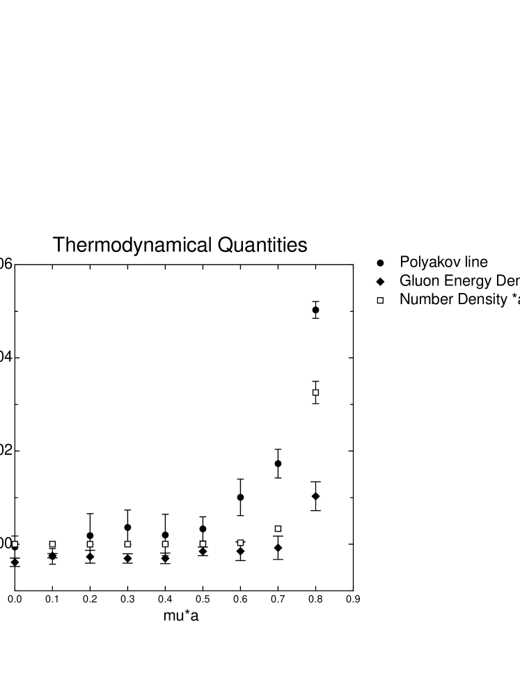
Figure 1: Polyakov line, gluon energy density, and baryon number density as a function of chemical Potential $\mu$.

4 Meson and Baryon

Because fundamental representation of the SU(2) is 2, baryon in the SU(2)-QCD is diquark state. Scalar diquark state and pseudo-scalar diquark state are given as $(C^{-1}\psi)^{T}\gamma_{5}\psi$ and $(C^{-1}\psi)^{T}{\bf 1}\psi$, respectively, with $C$ being charge conjugation matrix. Charge conjugation makes transform property of the diquark state look opposite to the ordinary combination of the scalar $\bar{\psi}{\bf 1}\psi$ and pseudo scalar $\bar{\psi}\gamma_{5}\psi$. We denote scalar diquark state and pseudo-scalar diquark state as b5b and b1b, respectively, for the abbreviation.

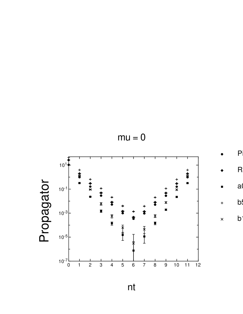
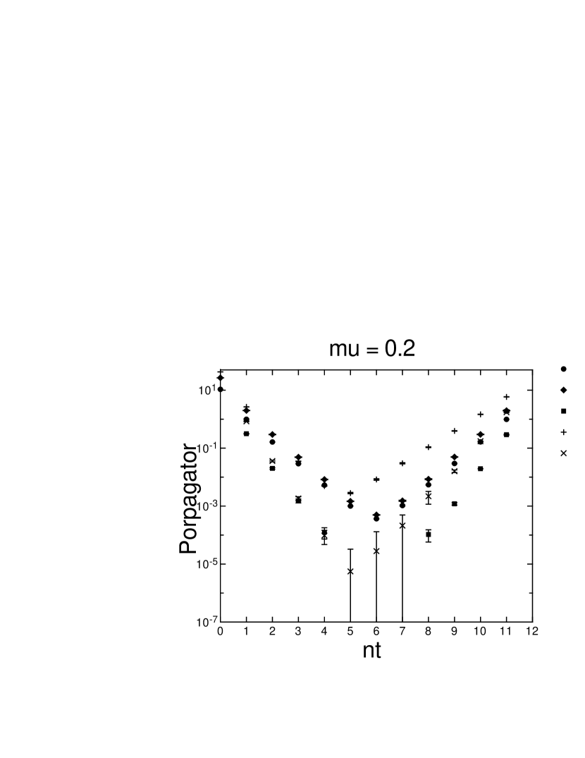
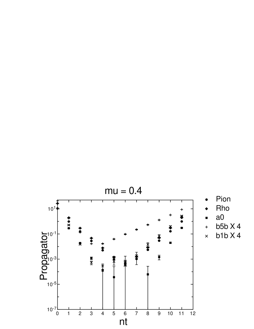
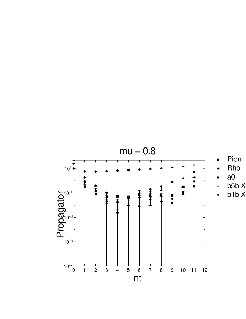
Figure 2: Propagators of mesons and diquarks of $4^{3}\times 12$ lattice at $\beta=0.70$ and $\kappa=0.150$. In order to avoid overplot of the data, diquark propagators are shifted 4 times.

We evaluate propagators of the pseudo scalar iso vector meson, $\pi$, the scalar iso vector meson, $a_{0}$, vector meson, $\rho$, pseudo scalar diquark (b1b) and scalar diquark (b5b). With vanishing chemical potential, the correlator of the $\pi$ and scalar diquark degenerate and so do $a_{0}$ and pseudo scalar diquark. Because meson has no net baryon number, effect of the chemical potential is expected to appear in the meson propagator only through the mass. On the other hands, baryon (diquark) has definite baryon number; Hence, in addition to the change of the mass, the affect of the finite chemical potential on the particle and antiparticle is in opposite sign, which causes the asymmetry of the propagator in time direction. With a finite chemical potential $\mu$, propagator of diquark, $G_{b1b}(x,x^{\prime})$ and $G_{b5b}(x,x^{\prime})$, should behave as,

$$G_{b*b}(t,\mu)=G_{b*b}(T-t,-\mu),$$

in contrast to the meson propagator,

$$G_{m}(t,\mu)=G_{m}(T-t,\mu)$$

with $T$ being lattice size in the time direction.

Figure 2 shows propagators of mesons and diquarks. At $\mu=0$, as expected, pseudo scalar $\pi$ and scalar diquark (b5b) and scalar $a_{0}$ and pseudo scalar diquark coincide, respectively (in Fig.2, to avoid the overplot, diquark propagators are shifted by factor 4). With finite chemical potential, asymmetry of the diquark propagators in time direction and anti-time direction become stronger with $\mu$. On the other hand, meson propagators keeps symmetric in $n_{t}$. Hence, in our calculation, effect of the finite chemical potential works appropriately on the hadron propagators. Hands [6], reported that with finite chemical potential, propagator of the scalar diquark (b5b) and pseudo scalar diquark (b1b) become parallel and they proposed the interpretation that both diquark states give the same spectra and the difference corresponds to the diquark condensation. However, at least the present statistics, our results do not give the the diquark propagators in parallel.

5 CONCLUDING REMARKS

We present numerical study of SU(2)-QCD with the chemical potential on lattice with Wilson fermions. Although the lattice is not large, behaviors of the thermodynamical quantities suggest that we are at around the confinement/deconfinement phase transition. Though the change of the propagator as a function of the chemical potential $\mu$ is almost consistent with the results of [6], however, the spectrum of the diquarks seem to be different. But we need more statistics to conclude definite results. Estimation of the mass as a function of the chemical potential in the chiral limit is now in progress.

In our calculation, numerical convergence becomes worse and worse with larger chemical potential and at $\mu=1.0$ vanishing determinant makes simulation break-down. We are adopting the algorithm based on the exact calculation of the ratio of fermion determinant. Therefore, we can analyze the change of the distribution of eigenvalues of the fermion matrix with finite chemical potential [9]. Investigation of the physical meaning of the numerical instability and distribution of the eigenvalue are also our next task.

6 Acknowledgment

This work is supported by Grant-in-Aide for Scientific Research by Monbu-Kagaku-sho, Japan (No.11440080 and No. 12554008). Simulations were performed on SR8000 at IMC, Hiroshima University, SX5 at RCNP, Osaka university, SR8000 at KEK and VPP5000 at Science Information Processing Center, Tsukuba university.

7 Appendix

We adopt an algorithm where the ratio of the determinant,

$$\frac{\mbox{det}W(U+\Delta U)}{\mbox{det}W(U)}=\mbox{det}(I+W(U)^{-1}\Delta W)$$ (6)

is evaluated explicitly at each Metropolis update process, $U\rightarrow U+\Delta U$, where $\Delta W\equiv W(U+\Delta U)-W(U)$ [10]. An essential ingredient of the algorithm is Woodbury formula,

$$(W+\Delta W)^{-1}=W^{-1}-W^{-1}\Delta W(I+W^{-1}\Delta W)^{-1}W^{-1}.$$ (7)

Suppose we update link variables $U_{\mu}(x)$s only on a subset $H$ of whole lattice. Though $\Delta W\neq 0$ only on $H$, Woodbury formula (7) still holds on $H$, and in this case, we can get the ratio of the fermion determinant as far as $U_{\mu}(x)$s are locally updated only inside $H$. We take a $2^{4}$ hypercube as $H$. When we move to the next hypercube, $(W^{-1})_{H}$’s are initialized by CG method.

We employ an algorithm which takes into account the ratio of fermion determinant exactly, and has large Markov step, but we suffer from numerical instability at about $\mu=1.0$

References

- [1] H. Satz, hep-ph/0009099.
- [2] A. Nakamura, Phys. Lett., 149B (1984) 391.
- [3] Z. Fodor and S. D. Katz,hep-lat/0106002.
- [4] J. B. Kogut et al., Nucl. Phys. B582 (2000) 477; D. T. Son and M. A. Stephanov, hep-ph/0005225, J. B. Kogut, M. A. Stephanov and D. Toublan, Phys. Lett. B464 (1999) 183.
- [5] M.-P. Lombardo, hep-lat/9907025; hep-lat/9906006.
- [6] S. Hands, J. B. Kogut, M-P. Lombardo and S. E. Morrison, Nucl. Phys. B558 (1999) 327; S. Morrison and S. Hands, hep-lat/9902012; S. Hands et al., hep-lat/0006018; S. J. Hands, J. B. Kogut, S. E. Morrison, D. K. Sinclair, hep-lat/0010028.
- [7] K. Rajagopal and F. Wilczek, hep-ph/0011333.
- [8] A. Nakamura, Acta. Phys. Pol. B16 (1985) 635; P. Hasenfratz and F. Karsch, Phys. Lett, 125B (1983) 308.
- [9] S. Muroya, A. Nakamura and C. Nonaka, Nucl. Phys., Nucl. Phys. B Proc. Suppl. 94(2001)469.
- [10] I. Barbour et al., J. Comput. Phys. 68 (1987) 227; A. Nakamura et al., Comm. Phys. Comm. 51 (1988) 301; Ph. de Forcrand et al., Phys. Rev. Lett., 58 (1987) 2011.