TWO-POTENTIAL APPROACH TO MULTI-DIMENSIONAL TUNNELING

Abstract

We consider tunneling to the continuum in a multi-dimensional potential. It is demonstrate that this problem can be treated as two separate problems: a) a bound state and b) a non-resonance scattering problem, by a proper splitting of the potential into two components. Finally we obtain the resonance energy and the partial tunneling widths in terms of the bound and the scattering state wave functions. This result can be used in a variety of tunneling problems. As an application we consider the ionization of atomic states by an external field. We obtain very simple analytical expressions for the tunneling width and for the angular distribution of tunneling electrons. It is shown that the angular spread of electrons in the final state is determined by the semi-classical traversal tunneling time.

1 Introduction

This paper is devoted to the memory of Michael Marinov, my friend and collaborator. Within the scope of his broad scientific activity Michael paid special attention to different aspects of quantum mechanical tunneling, as for instance to the coherent and quantum oscillation effects in tunneling processes,[1, 2] and to the traversal tunneling time.[3, 4] In particular Michael was interested in a semi-classical description of multi-dimensional tunneling. Our frequent discussions of this subject were very illuminating and helpful to me, especially in relation with the two-potential approach to multi-dimensional tunneling, which I shall present below.

It is well known that propagation through classically forbidden domains has been extensively studied since the early days of quantum mechanics. Yet, its exact treatment still remains very complicated and often not practical, in particular for the multi-dimensional case. The treatment of the tunneling problem can be essentially simplified by reducing it to two separate problems: a bound state plus a non-resonance scattering state. This can be done consistently in the two-potential approach (TPA).[5]^-[7] This approach provides better physical insight than other existing approximation methods, and it is simple and very accurate. It was originally derived by us for the one-dimensional case. Here we present an extension of TPA to many degrees of freedom and its application to ionization of atomic states.

2 General formalism

Consider a quantum system in a multi-dimensional space, described by the Schrödinger equation (we have adapted units where $\hbar=1$)

$$i{\partial\over\partial t}|\Psi(t)\rangle=[K+V({\mbox{\boldmath$x$}})]|\Psi(t)\rangle,$$ (1)

where ${\mbox{\boldmath$x$}}=\{x_{1},x_{2},\ldots,x_{n}\}$, $K={\mbox{\boldmath$\nabla$}}^{2}/2m$ is the kinetic energy term and $V({\mbox{\boldmath$x$}})$ is a multi-dimensional potential. The latter contains a barrier that divides the entire space into two domains (the “inner” and the “outer” one), such that the classical motion of the system in the inner domain is confined. Yet this does not hold for the quantum mechanical motion of this system. It is well known that any quantum state with a positive energy, localized initially inside the inner domain, tunnels to continuum (the outer domain) through the barrier. If the time-dependence of this process is dominated by its exponential component, we have a quasi-stationary (resonance) state. Below we describe a simple and consistent procedure for treatment of such multi-dimensional quasi-stationary states, which represents a generalization of the TPA, developed in Refs.  [5]– [7] for one-dimensional case.

Let us first introduce a hyper-surface $\Sigma$ inside the potential barrier, which separates the whole space into the inner and the outer regions, as shown schematically in Fig. 1.

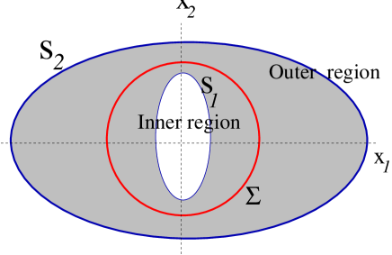
Figure 1: An example of the separation between the inner and the outer regions for a two-dimensional potential. $S_{1}$ and $S_{2}$ denote the equipotential lines for the energy $E_{0}$, Eq. (2). The shaded space correspond to the classically forbidden region. The separation line $\Sigma$ is taken as a circle.

Respectively, the potential $V({\mbox{\boldmath$x$}})$ can be represented as a sum of two components, $V({\mbox{\boldmath$x$}})=U({\mbox{\boldmath$x$}})+W({\mbox{\boldmath$x$}})$. The first component $U({\mbox{\boldmath$x$}})$ is defined in such a way that $U({\mbox{\boldmath$x$}})=V({\mbox{\boldmath$x$}})$ in the inner region, and $U({\mbox{\boldmath$x$}})=U_{0}$ in the outer region, where $U_{0}$ is the minimal value of $V({\mbox{\boldmath$x$}})$ on the hyper-surface, $U_{0}=$min $V({\mbox{\boldmath$x$}}\in\Sigma$). Respectively, the potential $W({\mbox{\boldmath$x$}})=0$ in the inner region, and $W({\mbox{\boldmath$x$}})=V({\mbox{\boldmath$x$}})-U_{0}$ in the outer region.

We start with the bound state $\Phi_{0}({\mbox{\boldmath$x$}})$ of the “inner” potential,

$$(K+U)|\Phi_{0}\rangle=E_{0}|\Phi_{0}\rangle\,,$$ (2)

where $E_{0}<U_{0}$. The potential $W({\mbox{\boldmath$x$}})$ is switched on at $t=0$. Then the state $|\Phi_{0}\rangle$ becomes the wave packet

$$\Psi({\mbox{\boldmath$x$}},t)=b_{0}(t)\Phi_{0}({\mbox{\boldmath$x$}})e^{-iE_{0}t}+\int b_{{\mbox{\boldmath$\scriptstyle k$}}}(t)\Phi_{{\mbox{\boldmath$\scriptstyle k$}}}({\mbox{\boldmath$x$}})e^{-iE_{{\mbox{\boldmath$\scriptstyle k$}}}t}\frac{d{\mbox{\boldmath$k$}}}{(2\pi)^{n}}$$ (3)

where $b_{0}(t),b_{{\mbox{\boldmath$\scriptstyle k$}}}(t)$ are the probability amplitudes of finding the system in the corresponding eigenstates $|\Phi_{0,{\mbox{\boldmath$\scriptstyle k$}}}\rangle$ of the Hamiltonian $H_{0}=K+U$. For simplicity we assume that the potential $U({\mbox{\boldmath$x$}})$ contains only one bound state $|\Phi_{0}\rangle$ corresponding to the energy $E_{0}$, Eq. (2). The amplitudes $b_{0}(t),\,b_{{\mbox{\boldmath$\scriptstyle k$}}}(t)$ can be found from the Schrödinger equation $i\partial_{t}|\Psi\rangle=(H_{0}+W)|\Psi\rangle$, supplemented with the initial conditions: $b_{0}(t)=1$, $b_{{\mbox{\boldmath$\scriptstyle k$}}}(0)=0$.

If the state $|\Psi(t)\rangle$ is a metastable one, the probability of finding the system inside the inner region drops down exponentially: $|b_{0}(t)|^{2}\sim e^{-\Gamma t}$, where $\Gamma$ is the width of this state. This implies that $\Gamma$ is determined by the exponential component of the amplitude $b_{0}(t)$. The latter corresponds to a pole in the complex $E$-plane of the Laplace transformed amplitude $\tilde{b}_{0}(E)$:

$$\tilde{b}_{0}(E)=\int_{0}^{\infty}e^{iEt}\,b_{0}(t)\,dt$$ (4)

The amplitude $\tilde{b}_{0}(E)$ can be found from the Schrödinger equation by using the Green’s function technique. We obtain: [6]

$$\tilde{b}_{0}(E)=\frac{i}{E-E_{0}-\langle\Phi_{0}|W|\Phi_{0}\rangle-\langle\Phi_{0}|W\tilde{G}(E)W|\Phi_{0}\rangle}$$ (5)

where the Green’s function $\tilde{G}$ is given by

$$\tilde{G}(E)=G_{0}(E)(1+\tilde{W}\tilde{G}(E)),$$ (6)

and

$$G_{0}(E)=\frac{1-\Lambda}{E+U_{0}-K-U},\qquad\Lambda=|\Phi_{0}\rangle\langle\Phi_{0}|\;.$$ (7)

Here $\tilde{W}({\mbox{\boldmath$x$}})=W({\mbox{\boldmath$x$}})+U_{0}$ is the outer component of the potential $V({\mbox{\boldmath$x$}})$. Note that Eqs. (5)- (7) represent the standard perturbation theory, except for the “renormalized” distortion potential, i.e. $W({\mbox{\boldmath$x$}})$ is replaced by $\tilde{W}({\mbox{\boldmath$x$}})$ in the Green’s function $\tilde{G}$, Eq. (6). [6]

It follows from Eq. (5) that a pole of $\tilde{b}_{0}(E)$ (at $E=E_{r}-i\Gamma/2$), that determines the energy $E_{r}$ and the width $\Gamma$ of a quasi-stationary state, is given by the equation

$$E=E_{0}+\langle\Phi_{0}|W|\Phi_{0}\rangle+\langle\Phi_{0}|W\tilde{G}(E)W|\Phi_{0}\rangle\,.$$ (8)

One can easily show [6] that Eq. (8) determines in fact, the poles in the total Green’s function $G(E)=(E-K-V)^{-1}$ at complex $E$. Since their position depends only on the potential $V({\mbox{\boldmath$x$}})$, the resonance energy $E_{r}$ and the width $\Gamma$, given by Eq. (8) are independent of the choice of the separation hyper-surface, $\Sigma$.

One can solve Eq. (8) perturbatively by using the standard Born series for the Green’s function

$$\tilde{G}=G_{0}+G_{0}\tilde{W}G_{0}+G_{0}\tilde{W}G_{0}\tilde{W}G_{0}+\cdots\ .$$ (9)

Substituting Eq. (9) into Eq. (8) we obtain the corresponding series for $E_{r}-i\Gamma/2$. Yet, such a series converges very slowly.

For this reason we proposed in Ref.  [6] a different expansion for $\tilde{G}$, which converges much faster than the Born series. This is achieved by expanding $\tilde{G}$ in powers of the Greens function $G_{\tilde{W}}$,

$$G_{\tilde{W}}(E)=\frac{1}{E-K-\tilde{W}}\,,$$ (10)

corresponding to the outer potential $\tilde{W}$, instead of $G_{0}$, Eqs. (7), (9), which corresponds to the inner potential $U$. One then obtains from Eqs. (6), (10)

$$\tilde{G}=G_{\tilde{W}}+G_{\tilde{W}}(U-U_{0})\tilde{G}-\tilde{G}_{\tilde{W}}\Lambda(1+\tilde{W}\tilde{G})$$ (11)

Iterating Eq. (11) in powers of $G_{\tilde{W}}$ and then substituting the result into Eq. (8) we obtain the desirable perturbative expansion for the resonant energy and the width. Using simple physical reasonings and direct evaluation of higher order terms for one dimensional case, we demonstrated in Refs.  [6],  [7] that this expansion converges very fast, so that $\tilde{G}$ is well approximated by the first term $G_{\tilde{W}}$. In this case Eq. (8) becomes:

$$E=E_{0}+\langle\Phi_{0}|W|\Phi_{0}\rangle+\langle\Phi_{0}|WG_{\tilde{W}}(E)W|\Phi_{0}\rangle,$$ (12)

Solving Eq. (12) for complex $E=E_{r}-i\Gamma/2$ we find the resonance energy $E_{r}$ and the width $\Gamma$ with a high accuracy (of order $\Gamma/U_{0}$).

Let us assume that that $|\Delta|,\,\Gamma\ll E_{0}$, where $\Delta=E_{r}-E_{0}$ is the energy shift. In this case we can solve Eq. (12) iteratively by replacing the argument $E$ in the Green’s function by $E_{0}$:

$$E=E_{0}+\langle\Phi_{0}|W|\Phi_{0}\rangle+\langle\Phi_{0}|WG_{\tilde{W}}(E_{0})W|\Phi_{0}\rangle\,.$$ (13)

Equation (13) can be significantly simplified. Indeed, the Green’s function $G_{\tilde{W}}$ satisfies the Schrödinger equation

$$\left[E_{0}-K-\tilde{W}({\mbox{\boldmath$x$}})\right]G_{\tilde{W}}(E;{\mbox{\boldmath$x$}},{\mbox{\boldmath$x$}}^{\prime})=\delta({\mbox{\boldmath$x$}}-{\mbox{\boldmath$x$}}^{\prime})\,,$$ (14)

which can be rewritten as

$$W({\mbox{\boldmath$x$}})G_{\tilde{W}}(E_{0};{\mbox{\boldmath$x$}},{\mbox{\boldmath$x$}}^{\prime})=\left(E_{0}-U_{0}-{{\mbox{\boldmath$\nabla$}}^{2}\over 2m}\right)G_{\tilde{W}}(E_{0};{\mbox{\boldmath$x$}},{\mbox{\boldmath$x$}}^{\prime})-\delta({\mbox{\boldmath$x$}}-{\mbox{\boldmath$x$}}^{\prime})\ .$$ (15)

Substituting Eq. (15) into Eq. (13) we find that the corresponding contribution from the kinetic energy term (${\mbox{\boldmath$\nabla$}}^{2}/2m$) can be transformed as

$$\Phi_{0}({\mbox{\boldmath$x$}}){\mbox{\boldmath$\nabla$}}^{2}G_{\tilde{W}}(E_{0};{\mbox{\boldmath$x$}},{\mbox{\boldmath$x$}}^{\prime})={\mbox{\boldmath$\nabla$}}(\Phi_{0}{\mbox{\boldmath$\nabla$}}G_{\tilde{W}})-{\mbox{\boldmath$\nabla$}}(G_{\tilde{W}}{\mbox{\boldmath$\nabla$}}\Phi_{0})+G_{\tilde{W}}{\mbox{\boldmath$\nabla$}}^{2}\Phi_{0}$$ (16)

In addition, the potential $W({\mbox{\boldmath$x$}})$ is zero in the inner region, so that the integration over ${\mbox{\boldmath$x$}},{\mbox{\boldmath$x$}}^{\prime}$ in the matrix elements (13) takes place only in the outer region, ${\cal R}_{out}$. Then using Eq. (16) and the Gauss theorem we find

$$\int_{{\cal R}_{out}}\Phi_{0}(x){\mbox{\boldmath$\nabla$}}^{2}G_{\tilde{W}}(E_{0};x,x^{\prime})d{\mbox{\boldmath$x$}} = \int_{\Sigma}\left[\,G_{\tilde{W}}{\mbox{\boldmath$\nabla$}}_{{\mbox{\boldmath$\scriptstyle n$}}}\Phi_{0}-\Phi_{0}{\mbox{\boldmath$\nabla$}}_{{\mbox{\boldmath$\scriptstyle n$}}}G_{\tilde{W}}\right]d\sigma$$ (17)

$$+ \int_{{\cal R}_{out}}G_{\tilde{W}}{\mbox{\boldmath$\nabla$}}^{2}\Phi_{0}d{\mbox{\boldmath$x$}}$$

Since the wave function of the (inner) bound state in the outer region satisfies the Schrödinger equation with the potential $U_{0}$, the last term in Eq. (17) can be rewritten as

$$\int_{{\cal R}_{out}}G_{\tilde{W}}{\mbox{\boldmath$\nabla$}}^{2}\Phi_{0}d{\mbox{\boldmath$x$}}=2m(U_{0}-E_{0})\int_{{\cal R}_{out}}G_{\tilde{W}}\Phi_{0}d{\mbox{\boldmath$x$}}\ ,$$ (18)

Using Eqs. (15), (17), (18) we then obtain

$$\int\Phi_{0}(x)W({\mbox{\boldmath$x$}})G_{\tilde{W}}(E_{0};x,x^{\prime})d{\mbox{\boldmath$x$}}={1\over 2m}\int\limits_{\Sigma}\left[\,G_{\tilde{W}}{\mbox{\boldmath$\nabla$}}_{{\mbox{\boldmath$\scriptstyle n$}}}\Phi_{0}-\Phi_{0}{\mbox{\boldmath$\nabla$}}_{{\mbox{\boldmath$\scriptstyle n$}}}G_{\tilde{W}}\right]d\sigma-\Phi_{0}({\mbox{\boldmath$x$}}^{\prime})$$ (19)

Substituting Eq. (19) into Eq. (13) we find that the latter can be rewritten as

$$E=E_{0}-{1\over 2m}\int_{{\mbox{\boldmath$\scriptstyle x$}}\in\Sigma}\Phi_{0}({\mbox{\boldmath$x$}})\stackrel{{\scriptstyle\leftrightarrow}}{{{\mbox{\boldmath$\nabla$}}}}_{{\mbox{\boldmath$\scriptstyle n$}}}G_{\tilde{W}}(E_{0};{\mbox{\boldmath$x$}},{\mbox{\boldmath$x$}}^{\prime})W({\mbox{\boldmath$x$}}^{\prime})\Phi_{0}({\mbox{\boldmath$x$}}^{\prime})d\sigma d\sigma^{\prime}\ ,$$ (20)

where $\stackrel{{\scriptstyle\leftrightarrow}}{{{\mbox{\boldmath$\nabla$}}}}$ means the gradient on the right minus the gradient on the left.

The ${\mbox{\boldmath$x$}}^{\prime}$ integration can be carried out in the same way by using Eqs. (15)-(18). Again, the ${\mbox{\boldmath$\nabla$}}^{2}\Phi_{0}({\mbox{\boldmath$x$}}^{\prime})$ term cancels as well as the $\delta$-function contribution. Finally we obtain that the resonance energy and the width are expressed through a double integral over the hyper-surface $\Sigma$

$$E=E_{0}-{1\over(2m)^{2}}\int_{{\mbox{\boldmath$\scriptstyle x$}},{\mbox{\boldmath$\scriptstyle x$}}^{\prime}\in\Sigma}\Phi_{0}({\mbox{\boldmath$x$}})\stackrel{{\scriptstyle\leftrightarrow}}{{{\mbox{\boldmath$\nabla$}}}}_{{\mbox{\boldmath$\scriptstyle n$}}}G_{\tilde{W}}(E_{0};{\mbox{\boldmath$x$}},{\mbox{\boldmath$x$}}^{\prime})\stackrel{{\scriptstyle\leftrightarrow}}{{{\mbox{\boldmath$\nabla$}}}}_{{\mbox{\boldmath$\scriptstyle n$}}^{\prime}}\Phi_{0}({\mbox{\boldmath$x$}}^{\prime})d\sigma d\sigma^{\prime}\,.$$ (21)

The resonance width $\Gamma$ can be easily obtained from Eq. (21) by taking the spectral representation for the Green’s function,

$$G_{\tilde{W}}=\int{|\varphi_{{\mbox{\boldmath$\scriptstyle k$}}}\rangle\langle\varphi_{{\mbox{\boldmath$\scriptstyle k$}}}|\over E_{0}-E_{{\mbox{\boldmath$\scriptstyle k$}}}-i\eta}\,{d{\mbox{\boldmath$k$}}\over(2\pi)^{n}}\ ,$$ (22)

where $E_{{\mbox{\boldmath$\scriptstyle k$}}}={\mbox{\boldmath$k$}}^{2}/2m$ and $\varphi_{{\mbox{\boldmath$\scriptstyle k$}}}$ are the eigenstates of the “outer” Hamiltonian corresponding to non-resonance scattering states.

$$[K+\tilde{W}({\mbox{\boldmath$x$}})]\varphi_{{\mbox{\boldmath$\scriptstyle k$}}}({\mbox{\boldmath$x$}})=E_{{\mbox{\boldmath$\scriptstyle k$}}}\varphi_{{\mbox{\boldmath$\scriptstyle k$}}}({\mbox{\boldmath$x$}})\,,$$ (23)

Using Eqs. (21), (22) one obtains the total width as an integral over the partial width $\Gamma_{{\mbox{\boldmath$\scriptstyle k$}}}$

$$\Gamma=\left.\int\Gamma_{{\mbox{\boldmath$\scriptstyle k$}}}{dk_{1}\cdots dk_{n-1}\over(2\pi)^{n-1}}\right|_{|{\mbox{\boldmath$\scriptstyle k$}}|=k_{0}}$$ (24)

where $k_{0}=\sqrt{2mE_{0}}$ and

$$\Gamma_{{\mbox{\boldmath$\scriptstyle k$}}}={1\over 4mk_{n}}\left|\int_{{\mbox{\boldmath$\scriptstyle x$}}\in\Sigma}\Phi_{0}({\mbox{\boldmath$x$}})\stackrel{{\scriptstyle\leftrightarrow}}{{{\mbox{\boldmath$\nabla$}}}}_{{\mbox{\boldmath$\scriptstyle n$}}}\varphi_{{\mbox{\boldmath$\scriptstyle k$}}}({\mbox{\boldmath$x$}})d\sigma\right|^{2}_{|{\mbox{\boldmath$\scriptstyle k$}}|=k_{0}}\ .$$ (25)

Equations. (24) and (25) represent our final result for the total and partial tunneling widths of the resonance state with energy $E_{r}=E_{0}$, Eq. (2) .  The latter is the energy of a pure bound state $\Phi_{0}$ in the inner potential $U({\mbox{\boldmath$x$}})$. Both $\Gamma_{\mbox{\boldmath$\scriptstyle k$}}$ and $E_{0}$ are independent of the hyper-surface $\Sigma$ (up to the terms of the order of $\Gamma/U_{0}$), providing that $\Sigma$ is taken far away from the equipotential surfaces $V({\mbox{\boldmath$x$}})=E_{0}$ . [7]

Equations. (2), (24), (25) considerably simplify the multi-dimensional tunneling problem, by reducing it to the bound state problem. The latter can be treated with standard techniques. Some examples of applications of our method are given below.

3 Ionization of bound state in semi-classical approximation

Consider a three-dimensional potential $u({\mbox{\boldmath$r$}})$, which contains a bound state $\phi_{0}({\mbox{\boldmath$r$}})$ with the energy $\epsilon_{0}<0$. Let us superimpose an additional potential $v(x)$, depending on the coordinate $x$. We assume that $v(x)$ ionizes the bound state $\phi_{0}$, i.e. $u({\mbox{\boldmath$r$}})+v(x)<\epsilon_{0}$ for $x\to\infty$. We also assume that $u({\mbox{\boldmath$r$}})$ and $v(x)$ do not overlap, such that $u({\mbox{\boldmath$r$}})\approx 0$ for $x>x_{1}$ and $v(x)\approx 0$ for $x<x_{2}$, where $x_{1}<x_{2}$. Now taking the separation hyper-surface $\Sigma$ as a plane, $x=x_{0}$ where $x_{1}<x_{0}<x_{2}$, we can identify $u({\mbox{\boldmath$r$}})$ and $v(x)$ with the inner and the outer potentials, $U$ and $\tilde{W}$, Eqs. (2), (23). Then the bound state wave function $\phi_{0}({\mbox{\boldmath$r$}})$ coincides with the inner wave function $\Phi_{0}$; Eq. (2).

Providing that $v(x)$ is a function of $x$ only, the outer wave function, Eq. (23) can be written as a product $\varphi_{{\mbox{\boldmath$\scriptstyle k$}}}({\mbox{\boldmath$r$}})=\exp(i{\mbox{\boldmath$q$}}{\mbox{\boldmath$b$}})\chi_{k}(x)$, with ${\mbox{\boldmath$r$}}=(x,{\mbox{\boldmath$b$}})$, ${\mbox{\boldmath$k$}}=(k,{\mbox{\boldmath$q$}})$ and ${\mbox{\boldmath$k$}}^{2}=2m(u_{0}+\epsilon_{0})$, where $u_{0}=-v(x\to\infty)$. As a result, Eq. (25) for the partial width $\Gamma_{q}$ reads

$$\Gamma_{q}=\frac{1}{4m\bar{k}}\left|\int e^{i{\mbox{\boldmath$\scriptstyle q$}}{\mbox{\boldmath$\scriptstyle b$}}}\left[\phi_{0}(x,{\mbox{\boldmath$b$}})\frac{\partial}{\partial x}\chi_{\bar{k}}(x)-\chi_{\bar{k}}(x)\frac{\partial}{\partial x}\phi_{0}(x,{\mbox{\boldmath$b$}})\right]d\,^{2}b\right|_{x=x_{0}}^{2}\ ,$$ (26)

where $\bar{k}=\sqrt{2m(u_{0}+\epsilon_{0})-{\mbox{\boldmath$q$}}^{2}}$. Respectively, the total width, Eq. (24), is given by

$$\Gamma=\int\Gamma_{q}\,\frac{d\,^{2}q}{(2\pi)^{2}}$$ (27)

Since $\chi_{\bar{k}}(x)$ is a non-resonant wave function, it falls down exponentially inside the barrier and can be evaluated by using the standard semi-classical approximation.[9] One can write

$$\chi_{\bar{k}}(x)=\sqrt{\frac{\bar{k}}{|\tilde{p}_{q}(x)|}}\,e^{-\!\int_{x}^{x_{f}}|\tilde{p}_{q}(x^{\prime})|dx^{\prime}}\ .$$ (28)

Here $\tilde{p}_{q}(x)=\sqrt{2m[\epsilon_{0}-v(x)]-q^{2}}$, and $x_{f}$ is the outer classical turning point, $\tilde{p}_{q}(x_{f})=0$.

The inner wave-function describes the bound state and therefore it decreases exponentially under the barrier, as well

$$\phi_{0}(x,{\mbox{\boldmath$b$}})\sim e^{-\!\int_{x_{i}}^{(x^{2}+{\mbox{\boldmath$\scriptstyle b$}}^{2})^{1/2}}|\tilde{p}(x^{\prime},{\mbox{\boldmath$\scriptstyle b$}})|dx^{\prime}}\,.$$ (29)

Here $|\tilde{p}(x,{\mbox{\boldmath$b$}})|=\sqrt{2m[\epsilon_{0}-u(x,{\mbox{\boldmath$b$}})]}$, and $x_{i}$ is the inner classical turning point. It follows from Eq. (29) that $\phi_{0}(x,{\mbox{\boldmath$b$}})$ decreases very quickly with $b$ so that only small $b$ contribute in the integral (26). Thus, we can approximate the inner wave function and its derivative as

$$\phi_{0}(x,{\mbox{\boldmath$b$}})\simeq\frac{x_{i}}{x}\,\phi_{0}(x_{i},0)\,e^{-\!\int_{x_{i}}^{x}|\tilde{p}(x^{\prime},0)|dx^{\prime}-|\tilde{p}(x,0)|{\mbox{\boldmath$\scriptstyle b$}}^{2}/2x}\;,$$ (30)

$$\frac{\partial\phi_{0}(x,{\mbox{\boldmath$b$}})}{\partial x}\simeq-|\tilde{p}(x,0)|\,\phi_{0}(x,{\mbox{\boldmath$b$}})\;.$$ (31)

Substituting Eqs. (28), (30), (31) into Eq. (26) we can perform the $b$-integration by using

$$\int e^{i{\mbox{\boldmath$\scriptstyle q$}}{\mbox{\boldmath$\scriptstyle b$}}}\,\phi_{0}(x_{0},{\mbox{\boldmath$b$}})d\,^{2}b=\frac{2\pi x_{i}}{|\tilde{p}(x_{0},0)|}\,\phi_{0}(x_{0},0)\,e^{-\!\int_{x_{i}}^{x_{0}}|\tilde{p}(x^{\prime},0)|dx^{\prime}-x_{0}{\mbox{\boldmath$\scriptstyle q$}}^{2}/2|\tilde{p}(x_{0},0)|}\,.$$ (32)

Since $x_{0}\gg x_{i}$ the exponent in Eq. (32) can be approximated as

$$\int_{x_{i}}^{x_{0}}|\tilde{p}(x^{\prime},0)|dx^{\prime}+\frac{x_{0}q^{2}}{2|\tilde{p}(x_{0},0)|}\approx\int_{x_{i}}^{x_{0}}[\tilde{p}^{2}(x^{\prime},0)+{\mbox{\boldmath$q$}}^{2}]^{1/2}dx^{\prime}$$ (33)

Now using Eqs. (32), (33), and $\partial\chi_{\bar{k}}/\partial x\simeq|\tilde{p}_{q}(x)|\chi_{\bar{k}}$, we obtain the following formula for the partial width,

$$\Gamma_{q}=\frac{4\pi^{2}x_{i}^{2}\phi_{0}^{2}(x_{i},0)}{m(2m|\epsilon_{0}|)^{1/2}}e^{-2\int_{x_{i}}^{x_{f}}p_{q}(x)dx}\,,$$ (34)

where

$$p_{q}(x)=\sqrt{2m[u(x,0)+v(x)-\epsilon_{0}]+{\mbox{\boldmath$q$}}^{2}}\,,$$ (35)

is the absolute value of the imaginary momentum in the direction of the external field.

4 Partial width and the tunneling time

In contrast with the one-dimensional tunneling, the final state in a multi-dimensional tunneling is highly degenerate. Hence, a tunneling particle can be found in different final states with the same total energy. In our case these are all the states with different lateral momenta $q$, leading to the angular distribution of a tunneling particle. Using our result for the partial width, Eq. (34), one easily finds that this distribution is of a Gaussian shape. Indeed, by expanding the exponent of Eq. (34) in powers of ${\mbox{\boldmath$q$}}^{2}$ we obtain

$$\int_{x_{i}}^{x_{f}}p_{q}(x)dx\simeq S(E_{0},x_{i},x_{f})+\frac{q^{2}}{2m}\int_{x_{i}}^{x_{f}}\frac{mdx}{p(x)}\,,$$ (36)

where $p(x)=p_{q=0}(x)$ and

$$S(\epsilon_{0},x_{i},x_{f})=\int_{x_{i}}^{x_{f}}p(x)dx$$ (37)

is the action in the classically forbidden region. Then Eq. (34) reads

$$\Gamma_{q}=\frac{4\pi^{2}x_{i}^{2}\phi_{0}^{2}(x_{i},0)}{m(2m|\epsilon_{0}|)^{1/2}}e^{-2S(\epsilon_{0},x_{i},x_{f})-\tau q^{2}/m}\,,$$ (38)

where

$$\tau=\int_{x_{i}}^{x_{f}}\frac{mdx}{|p(x)|}\,,$$ (39)

is the Büttiker-Landauer tunneling time.[10] The latter is assumed to be an amount of time, which a particle spends traversing a tunnel barrier. It appears, however, that such a quantity is not uniquely defined in one-dimensional tunneling.[11, 3] Yet, the situation is different for the multi-dimensional case. Our result, Eq. (38), shows that the Büttiker-Landauer traversal tunneling time $\tau$ is related to a well defined quantity, namely to the lateral spread of a tunneling particle ($r_{0}$). [4] Indeed, the latter corresponds to the inverse average lateral momentum, $r_{0}=1/<q>$, where $<q>=\sqrt{m/\tau}$ as obtained from Eq. (38).

The Gaussian shape of angular distribution of tunneling particles is a general phenomenon, which can be understood in the following way.[4] It is well known that the most probable tunneling path corresponds to the minimal action. In our case this path is along the direction of the external field. Therefore any momentum $q$, normal to this direction raises the action by a term proportional to the corresponding energy ${\mbox{\boldmath$q$}}^{2}/2m$. This leads to the Gaussian fall-off of the related probability distribution.

5 Total width and angular distribution of ionized particles

Substituting Eq. (38) into Eq. (27) and performing the $q$-integration, we obtain the following expression for the total width

$$\Gamma=\frac{\pi\,x_{i}^{2}\,\phi_{0}^{2}(x_{i},0)}{\tau\,(2m|\epsilon_{0}|)^{1/2}}\,e^{-2S(E_{0},x_{i},x_{f})}\;.$$ (40)

Using this result, Eq. (38) can be rewritten in a more compact form as

$$\Gamma_{{\mbox{\boldmath$\scriptstyle q$}}}={4\pi\over m}\,\Gamma\,\tau\,e^{-\tau{\mbox{\boldmath$\scriptstyle q$}}^{2}/m}$$ (41)

Let us consider two exemplifying applications of Eqs. (40), (41).

(a) Hydrogen atom

Consider the Hydrogen atom in the ground state under the electric field ${\cal E}$. We use the atomic units in which $m=1$, the ground state energy $\epsilon_{0}=-1/2$ and the ground state wave function $\phi_{0}(r)=\exp(-r)/\sqrt{\pi}$. In these units the inner and the outer potentials are: $u(r)=-1/r$ and $v(x)=-{\cal E}x$. Then the action $S$, Eq. (37) reads

$$S=\int_{x_{i}}^{x_{f}}\sqrt{1-\frac{2}{x}-2{\cal E}x}dx\simeq\int_{x_{i}}^{x_{f}}\sqrt{1-2{\cal E}x}dx-\int_{x_{i}}^{x_{f}}\frac{dx}{x\sqrt{1-2{\cal E}x}}\,.$$ (42)

Although the main contribution to the action is coming from large $x$, we have keep in (42) also the next term of expansion (see Ref.  [12]). Performing the integration in Eq. (42) we obtain for the action

$$S\simeq\frac{1}{3{\cal E}}+\ln\left(\frac{{\cal E}x_{i}}{2}\right)-\frac{x_{i}}{2}\ ,$$ (43)

where we assumed that ${\cal E}x_{i}\ll 1$. Respectively for the “tunneling” one obtains $\tau=1/{\cal E}$. Using these results we easily find from Eq. (40) the well-known result for the ionization width of the Hydrogen atom [12]

$$\Gamma={4\over{\cal E}}\,e^{-2/3{\cal E}}\,.$$ (44)

Respectively, the angular distribution of ionized electrons, Eq. (41), is

$$\Gamma_{\mbox{\boldmath$\scriptstyle q$}}={4\pi\over{\cal E}}\,\Gamma e^{-{\mbox{\boldmath$\scriptstyle q$}}^{2}/{\cal E}}\,.$$ (45)

(b) Potential well with short range forces

The bound $s$-state wave function of a short range potential at distances larger then the radius of the well $a$ has the following form

$$\phi_{0}(r)={A\sqrt{\kappa}\over r}\,e^{-\kappa r}\,,$$ (46)

where $\kappa=(2|\epsilon_{0}|)^{1/2}$ and $A$ is a dimensionless constant depending on the specific form of the well [12]. For instance, if $a\ll 1/\kappa$, then $A=(2\pi)^{-1/2}$.

Similar to the previous case we use the same units but now with $\kappa=1$. The action and the tunneling time are evaluated straightforwardly from Eqs. (37), (39) taking into account that the initial turning points are $x_{i}=a\to 0$. One finds

$$S = \int_{0}^{1/2{\cal E}}\sqrt{1-2{\cal E}x}dx={1\over 3{\cal E}}$$ (47)

$$\tau = \int_{0}^{1/2{\cal E}}{dx\over\sqrt{1-2{\cal E}x}}={1\over\ {\cal E}}$$ (48)

Using $x_{i}^{2}\phi_{0}^{2}(x_{i},0)=A^{2}$ one obtains from Eq. (40)

$$\Gamma=\pi A^{2}\,{\cal E}\,e^{-2/3{\cal E}}\,.$$ (49)

This coincides with the result obtained by Demkov and Drukarev,[12, 13] using a more complicated technique.

The angular distribution of ionized particles, Eq. (41), is

$$\Gamma_{\mbox{\boldmath$\scriptstyle q$}}=4\pi^{2}A^{2}e^{-2/3{\cal E}}e^{-{\mbox{\boldmath$\scriptstyle q$}}^{2}/{\cal E}}\,.$$ (50)

The same result was obtained earlier in Ref.  [4].

6 Summary

In this paper we extended the two-potential approach to quantum tunneling to a multi-dimensional case. We found simple expressions for the energy and the partial widths of a quasi-stationary state, initially localized inside a multi-dimensional potential. The partial width, which determines the distribution of tunneling particles in the final state, is given by an integral of the bound and non-resonant scattering wave functions over the hyper-surface taken inside the potential barrier.

We applied our results for the ionization of atomic states by an external field depending only on one of the coordinates. In this case we obtained very simple semi-classical expressions for the total ionization width and the angular distribution of tunneling electrons, valid for any initial state. We demonstrated that in the case of the Hydrogen atom and also for a short range potential our general expression for the total width produces the results, existing in the literature, but obtained with a more complicated calculations.

We also demonstrated that angular distribution of tunneling electrons in the final state falls off as a Gaussian function of the lateral momentum. The exponential is determined by the traversal semi-classical tunneling time.

References

References

• [1] S.A. Gurvitz and M.S. Marinov, Phys. Rev. A 40, 2166 (1989).
• [2] S.A. Gurvitz and M.S. Marinov, Phys. Lett. A 149, 173 (1990).
• [3] M.S. Marinov and B. Segev, Phys. Rev. A 55, 3585 (1997).
• [4] C. Bracher, W. Becker, S.A. Gurvitz, M. Kleber and M.S. Marinov, Am. J. Phys. 66, 38 (1998).
• [5] S.A. Gurvitz and G. Kalbermann, Phys. Rev. Lett. 59, 262 (1987).
• [6] S.A. Gurvitz, Phys. Rev. A 38, 1747 (1988).
• [7] S.A. Gurvitz, P.B. Semmes, W. Nazarewicz, and T. Vertse, to be submitted to Phys. Rev. C.
• [8] J. Bardeen, Phys. Rev. Lett. 6, 57 (1961).
• [9] L.I. Shiff, Quantum Mechanics (McGraw-Hill, New York, 1955).
• [10] M. Büttiker and R. Landauer, Phys. Rev. Lett. 49, 1739 (1982).
• [11] E.H. Hauge and J.A. Støvneng, Rev. Mod. Phys. 61, 917 (1989).
• [12] L.D. Landau and E.M. Lifshitz, Quantum Mechanics (Butterworth–Heinemann, Oxford, 1991), pp. 295-297.
• [13] Yu.N. Demkov and G.F. Drukarev, Sov. Phys. JETP 20, 614 (1965).