Time dependence of critical behavior in multifragmentation

Abstract

We study signatures of critical behavior in microscopic simulations of small, highly excited Lennard-Jones drops. We focus our attention on the behavior of the system at the time of fragment formation (which takes place in phase space) and compare the results with the corresponding ones obtained at asymptotic times (experimentally accessible). The four critical exponents ($\tau$,$\beta$, $\sigma$ and $\gamma$) found at fragmentation time have shown to be stable against time evolution, indicating that the asymptotic stage reflects accurately the physics at fragmentation time. Even though evidence of critical behavior arises from the calculations, we can not affirm that the system is performing a second order like phase transition.

The process of rapid expansion and fragmentation of highly excited drops attracts the attention of physicists in different areas, in particular in the field of nuclear physics. The possibility of facing a phase transition was initially triggered by the work of the Purdue Group [1] when the resulting fragment mass spectra of proton-nucleus colission was fitted by a power law like dependence. This has initiated a series of works focusing on the extraction of signals of critical behavior from both, experimental measurements as well as data resulting from numerical simulations [2, 3, 4, 5, 6, 7, 8]. In the experimental case the only information available corresponds to the asymptotic regime and the primordial fragments have to be reconstructed from this data by the application of different approximations [9]. In a series of works (see for example [10], [11]) critical exponents have been calculated from the analysis of the experimental fragment mass distributions. On the other hand, in the case of numerical simulations all the microscopic information is available at all times, and if appropriate fragment recognition algorithms are used, one can unveil the complex fragmentation mechanism. In this work we use the already presented Early Cluster Recognition Algorithm (ECRA) to recognize fragments [12]. The advantage of this methodology is that it is able to find, very early in the evolution, the partitions of the system that give rise to the asymptotic fragments. These partitions (ECRA clusters) are the most bound density fluctuations in phase space and has been proved to be the seeds of the asymptotic fragments [13, 14]. As all order correlations are available, it is possible to follow the evolution in time of the ECRA clusters and determine the time of fragment formation ($\tau_{ff})$ as the time at which these clusters attain microscopic stability. Once the distribution of ECRA clusters at $\tau_{ff}$ is known, we can look for signals of critical behavior and extract the values of the critical exponents $\tau$, $\beta$, $\sigma$ and $\gamma$ (for a definition of these critical exponents see section III) . We then test the stability of the values of these exponents as a function of time, checking if the values extracted at asymptotic times are similar to the ones obtained at $\tau_{ff}$. In this way, we try to determine if the asymptotic stage information properly characterize the state of the system at fragmentation time.

This work is organized as follows: In Section I we describe the model used to simulate the fragmentation process as well as the algorithms adopted to recognize the fragments. In Section II we will give a brief description of the scaling model applied to analyze the data extracted from simulations, as well as the behavior of the system near the critical point. In Section III we analyze the behavior of some signals of critical behavior at $\tau_{ff}$ and at asymptotic time. The selected signals of critical behavior are: the second moment of the fragment distribution ($M_{2}$), the normalized variance of the mass of the maximum fragment ($NVM$), the best power law fit to the fragment spectra according to the assumed scaling model (minimum $\chi^{2}$) and the critical exponents $\tau$, $\gamma$, $\beta$ and $\sigma$. Finally, in Section IV, conclusions are drawn.

I Computer Experiments

In previous works [13, 14, 15] we have already analyzed the dynamics of fragment formation and the caloric curve for excited drops made up of 147 particles interacting via a 6-12 Lennard Jones potential. The interaction potential reads:

$$V(r)=\left\{\begin{array}[]{ll}4\epsilon\left[\left(\frac{\sigma}{r}\right)^{12}-\left(\frac{\sigma}{r}\right)^{6}-\left(\frac{\sigma}{r_{c}}\right)^{12}+\left(\frac{\sigma}{r_{c}}\right)^{6}\right]&r<r_{c}\\ 0&r\geq r_{c}.\end{array}\right.$$ (1)

We took the cut-off radius as $r_{c}=3\sigma$. Energy and distance are measured in units of the potential well ($\epsilon$) and the distance at which the potential changes sign ($\sigma$), respectively. The unit of time used is: $t_{0}=\sqrt{\sigma^{2}m/48\epsilon}$. In our numerical experiments initial conditions where constructed using the already presented [13, 14] method of cutting spherical drops composed of 147 particles out of equilibrated, periodic, 512 particles per cell L.J. system. One of the key ingredients in the analysis of fragmentation is the determination of the time at which fragments are formed. This can be accomplished if a proper fragment recognition method is employed. In this paper, clusters are defined according to the ECRA algorithm [12] in which the fragments are related to the most bound density fluctuations in phase space, as was mentioned above. These fragments are referred as ECRA clusters. In this case fragments are given by the set of clusters $\{C_{i}\}$ for which the sum of the fragment internal energies attains its minimum value:

$${\{C_{i}\}} {=} {\hbox{min}}_{{\scriptstyle\{C_{i}\}}}{\textstyle{[E_{\{C_{i}\}}=\sum_{i}E_{int}^{C_{i}}]}}$$ (2)

$$E_{int}^{C_{i}} = [\sum_{j\in C_{i}}K_{j}^{c.m.}+\sum_{{j,k\in C_{i}}{j\leq k}}V_{j,k}]$$ (3)

where the sum in the first equation of (3) is over the clusters of the partition, $K_{j}^{c.m.}$ is the kinetic energy of particle $j$ measured in the center of mass frame of the cluster which contains particle $j$, and $V_{ij}$ stands for the inter-particle potential.

Another way of recognizing fragments is provided by the Minimum Spanning Tree (MST) algorithm[13, 14]. In this case, given two particles $i,j,$ they belong to a cluster $C$ if the following relation is satisfied:

$$i\in C\Longleftrightarrow\exists j\in C\text{ }/\text{ }r_{ij}\text{ }\leq r_{cl}$$ (4)

with $r_{ij}$ the interparticle distance and $r_{cl}$ the clusterization radius ( $r_{cl}\leq r_{c}=3\sigma)$. In our case, we took $r_{cl}=r_{c}$. It should be noticed that in this definition the correlations in momentum space between particles are completely disregarded.

The asymptotic fragments detected by MST algorithm are observables. On the other hand, the ECRA clusters, being defined in phase space, are observables only when they coincide with MST clusters. For earlier times they are usually embedded into the MST clusters. It has been shown [12, 13, 14, 16] that different properties of the ECRA fragments (for instance the average size of the maximum fragment, or the average multiplicity of fragments in given bins, etc.) become stable very early in the evolution, much earlier than the times of stabilization of the same quantities calculated from MST clusters. As already mentioned in the introduction, the time of fragment formation is associated to the time at which the ECRA clusters attain microscopic stability. This occurs when the system switches from a regime dominated by fragmentation to one in which the dominant decay mode is evaporation. In order to estimate this time ($\tau_{ff}$) we use the so called, Short Time Persistence (STP), in which we calculate the stability of the ECRA clusters against evaporation-fragmentation and coalescence. It is defined in the following way: at a given time $t$ we analyze each fragment $C_{i}^{t}$ of size $N_{i}^{t}$ by searching on all the fragments $C_{j}^{t+dt}$ present at time $t+dt$ for the biggest subset $N_{\max}]_{i}^{t+dt}$ of particles that belonged to $C_{i}^{t}.$ Then we assign to this fragment a value $STP_{d}=\frac{N_{\max}]_{i}^{t+dt}}{N_{i}^{t}}$. This term account for the ”evaporation-fragmentation process”, but on the other hand one has to take care of the cases in which the $N_{\max}]_{i}^{t+dt}$ does not constitute a free cluster but is embedded in a bigger fragment of mass $N_{i}^{t+dt}$. We include this effect by defining $STP_{i}=\frac{N_{\max}]_{i}^{t+dt}}{N_{i}^{t+dt}}$. Finally the Short Time Persistence reads :

$$STP(t,dt)=\left\langle\left\langle\frac{STP_{d}(t,dt)+STP_{i}(t,dt)}{2}\right\rangle_{m}\right\rangle_{e}$$ (5)

where $\left\langle...\right\rangle_{m}$ is the mass weighted average over all the fragments with size $N>3$. And $\left\langle...\right\rangle_{e}$ is the average over an ensemble of fragmentation events at a given energy $E$ or multiplicity $m$. From this definition it is clear that $STP\sim 1$ if the analyzed partition remains unaltered during $dt$ and, on the other hand, $STP\sim 0$ if its microscopic composition presents large changes during that lapse of time.

In Fig. 1 we show one typical calculation of this magnitude. This is for a very energetic case $E=2.65\epsilon$ for which a fast exponentially decaying spectrum is obtained. In this figure we show $STP(t,dt)$ as a function of $t$ and for different values of $dt$, namely $dt=0.5t_{0},1t_{0}.,1.5t_{0},2t_{0}$. The almost horizontal line denotes the reference value of $STP$ and corresponds to fragments undergoing only a simple evaporation process. In this way we say that when $STP$ crosses this line the behavior of the system goes, on the average, from fragmentation to evaporation, and we call this time $\tau_{ff}$. Using the above mentioned criteria we have obtained time-scales ranging from $\tau_{ff}\sim 75t_{0}$ for $E=-0.5\epsilon$ up to $\tau_{ff}\sim 10t_{0}$ for $E=3.7\epsilon$.

FIG. 1.: Short time persistence (STP) as function of time for four different values of dt (empty squares:$dt=0.5t_{0}$, full circles $1t_{0}$, empty triangles $1.5t_{0}$ and stars $2t_{0}$) and the reference value (solid line)

.

In the same way, but working with the fragments given by the MST algorithm we get the times of fragment emission $\tau_{fe}$. ,i.e. the times at which the clusters defined in q-space become stable. These times are much larger than the corresponding time of fragment formation ($\tau_{ff}$). For example, for $E=-0.5\epsilon$, $\tau_{fe}=100t_{0}$. We took as asymptotic time, ($\tau_{a}$), a value much larger that all the $\tau_{fe}$ calculated, i.e., $\tau_{a}=600t_{0}$.

Once we determine the time of fragment formation ($\tau_{ff}$) and the asymptotic time ($\tau_{a}$), it is possible to calculate the corresponding ECRA fragment mass distribution at $\tau_{ff}$ and compare it with the corresponding MST fragment mass spectra at $\tau_{a}$. The result of such a calculation are displayed in Fig. 2. Three typical mass spectra are shown: U-shaped in panel (a), power law like in (b) and exponential decaying one in (c). Filled circles denote the ECRA distributions at time of fragment formation and empty triangles the MST ones at asymptotic times. It can be notice that the resulting distributions are esentially the same.

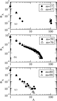
FIG. 2.: Three typical fragment distributions ($n_{A}$: number of clusters per particle of size $A$) corresponding to three different excitation energies and classified by their multiplicity values. Black circles correspond to ECRA fragment distributions at $\tau_{ff}$ and empty triangles to MST ones at asymptotic times. The values of $m$ indicate the multiplicity of the correspondig mass spectra . In panel (a) we show the U-shaped distributions (low excitation energies), in (b) the power law and in (c) the exponential decaying ones (high excitation energies)

.

II The Scaling Model: critical exponents and other signatures of criticality

The behavior of the system near its critical point can be described in terms of scaling laws. A widely used scaling model for the fragment mass distribution [10, 11, 19], based in renormalization group arguments [18], can be applied to this kind of problem. In this approach, the cluster distribution can be written as:

$$n_{A}(\epsilon)=q_{0}A^{-\tau}f(z),$$ (6)

where $n_{A}$ is the probability per particle of having a cluster of size $A$, $\tau$ is a critical exponent, $q_{0}$ a normalization constant and $f(z)$ a scaling function. This function depends on the distance to the critical point, $\epsilon$, and the mass number, $A$, via the combination [19]:

$$z=A^{\sigma}\epsilon,$$ (7)

with $\sigma$ a critical exponent. The distance to the critical point can be defined as $\epsilon=(T_{c}-T)/T_{c}$ for usual thermodynamic systems, and $\epsilon=(m_{c}-m)/m_{c}$ [10] for multifragmentation experiments.

At the critical point, $\epsilon=0$ (with $f(0)=1$ [19]), and the cluster mass distribution becames a power law:

$$n_{A}=q_{0}A^{-\tau},$$ (8)

where the normalization $q_{0}$ depends on $\tau$ via a Riemann $\zeta$ function [20]:

$$q_{0}=\frac{1}{\sum_{A}A^{1-\tau}}.$$ (9)

This dependence, coming from the normalization condition $M_{1}(\epsilon=0)=1$, should be taken into account to properly extract the critical exponent $\tau$ when fitting the cluster mass distribution to a power law.

A relevant quantity in the analysis of critical behavior is the second moment of the mass distribution:

$$M_{2}=\sum n_{A}A^{2}.$$ (10)

It has been shown (see for example [19]) that $M_{2}$ diverges at the critical point if the fragment distribution satisfies equation (6). This divergence can be described in terms of the critical exponent $\gamma$:

$$M_{2}(\epsilon)\propto\Gamma_{\pm}|\epsilon|^{-\gamma}.$$ (11)

Another relevant magnitude in the search of critical behavior is the normalized variance of the size of the biggest cluster $(NVM)$ [21], defined by:

$$NVM=\frac{<A_{max}-<A_{max}>>^{2}}{<A_{max}>}$$ (12)

where $A_{max}$ is the size of the biggest fragment and $<...>$ is the average over an ensemble of fragmentation events with a given multiplicity $m$. In [21] it was shown that it is a robust signature of critical fluctuations.

It is worth noting that for finite systems it is expected that scaling assumptions would be valid in a range of masses where finite size effects can be avoid and where the behavior of the system resembles the behavior of the infinite one.

We will see in the next section that for exploding LJ drops, the fragment distributions at $\tau_{ff}$ and $\tau_{a}$ follows the scaling model within a rather broad range of mass.

III Criticality Analysis

In what follows we search for critical behavior in our numerical simulations via the analysis of the fragment mass disttributions at both, fragmentation time $(\tau_{ff})$ and asymptotic times $(\tau_{a}).$

A Signals of critical behavior

We first calculate the normalized variance of the mass of the biggest fragment, $NVM$, and the second moment of the cluster mass distributions, $M_{2}$ as a function of the multiplicity, being the multiplicity a relevant observable in multifragmentation. The biggest fragment of each event should be removed for the liquid phase ($m<m_{c}$) in the calculation of $M_{2}$ [19]. Because we don’t know a priory the value of the critical multiplicity, the biggest fragment was excluded for all events [10].

The dependence of these magnitudes with the multiplicity is shown in Fig. 3 for the two times analyzed, $\tau_{ff}$ and $\tau_{a}$. It can be seen that both observables peak at, essentially, the same multiplicity value for each of the analized times. At $\tau_{ff}$, the NVM peaks for $m=60\pm 1$ [Fig. 3(a)] and the $M_{2}$ for $m=65\pm 4$ [Fig. 3(b)] (black triangles in both cases), whereas at asymptotic times, the magnitudes peak for $m=73\pm 1$ [Fig. 3(a)] and $m=77\pm 3$ [Fig. 3(b)] respectively (empty symbols). The higher multiplicity values at asymptotic times are due to evaporation processes undergone by the fragments, which increase the number of monomers and dimers. If we consider only fragments larger than $A=2$, both magnitudes ($M_{2}$ and $NVM$) peaks at the same value of multiplicity at both times. These results are compatible with the presence of critical behavior.

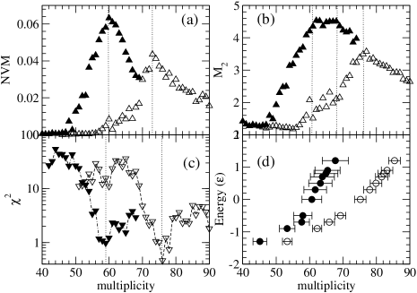
FIG. 3.: Normalized variance of the size of the maximum fragment (NVM) (a), second moment of the cluster distribution ($M_{2}$) (b), and best fit to a power law (with $q_{0}=q_{0}(\tau)$ via eq.(9)) (c) as function of the multiplicity for fragmentation time ($\tau_{ff}$), full triangles, and for asymptotic time ($\tau_{a}$), empty triangles. In (d) we can see average multiplicity and its standard desviation for each energy for $\tau_{ff}$ (full circles) and for $\tau_{a}$ (empty circles)

.

We will now search for a power law mass spectra according to the scaling model depicted in equation (6). As we have seen, the normalization $M_{1}(\epsilon=0)=1$ imposes a condition on $q_{0}$ such that $q_{0}=q_{0}(\tau)$ via a Riemann $\zeta$ function (eq.9). Therefore, if we want to find a power law behavior in the mass spectra obtained from the numerical simulations, we must fit them with equation (8) taking into account that the normalization, $q_{0}$, is given by equation (9). This method was successfully used in [10] both, for percolation and $Au+C$ multifragmentation. In our case, the best fitted mass spectra by $f(A,\tau)=q_{0}(\tau)A^{-\tau}$ determines the critical multiplicity whereas the corresponding slope in a log-log plot, the critical exponent $\tau$. The quality of the fitting procedure was measured via the standard $\chi^{2}$ coefficient (i.e., a minimum in $\chi^{2}$ corresponds to the best fit).

The fitting was performed in the mass range $0.02A_{tot}<A<0.15A_{tot}$ in order to avoid finite size effects. In Fig. 3(c) we can see the behavior of the coefficient $\chi^{2}$ as a function of the multiplicity as calculated at $\tau_{ff}$ (full triangles) and $\tau_{a}$ (open triangles). The minimum in $\chi^{2}$ signals the critical multiplicity: $m_{c}=59\pm 2$ for $\tau_{ff}$ and $m_{c}=76\pm 2$ for $\tau_{a}$. (The obtained values of $\tau$ from these fitting procedures will be reported in next sub-section). These results agree very well with those obtained above via $NVM$ and $M_{2}$.

The relation between the multiplicity and the energy of the system is plotted in Fig. 3(d). We can see that the critical multiplicities correspond mainly to energies around $E=0.3\epsilon$, energy for which the collective motion begins to be noticeable [17]. It can be seen that there is a one to one correspondence between the energy and the multiplicity and, moreover, starting right bellow $m_{c}$ the relation between energy and multiplicity becomes almost linear. This feature supports the use of multiplicity as a control parameter. A similar behavior was also observed in percolation for the relation between the multiplicity and the bond probability $p$.

All these signals show evidences of critical behavior not only at asymptotic times, when fragments are experimentally accessible, but also at fragmentation time, when the particles of the system are still interacting and they are recognized by the ECRA algorithm.

B Critical exponents

We now calculate four critical exponents: $\tau$, $\gamma$, $\sigma$, and $\beta$ at time of fragment formation ($\tau_{ff}$) and at asypmtotic time ($\tau_{a}$).

The calculation of $\tau$ is performed according to the procedure described in the previous section, i.e., finding the fragment mass spectra that is best fitted by a power law according to the scaling model in a given range of masses. From this calculations we got $\tau=2.18\pm 0.03$ for both times, $\tau_{ff}$ and $\tau_{a}$. The biggest fragment of each event was excluded when generating the average cluster distribution of a given multiplicity [10]. We can see that the resulting value of $\tau$ does not depend on the fit range as long as we stay in the range $0.02A_{tot}<A<0.15A_{tot}$, where finite size effects are not important. The cluster mass distributions at the critical multiplicity and their corresponding fits are shown in Fig. 4(a) for $\tau_{ff}$ and Fig. 5(a) for $\tau_{a}$.

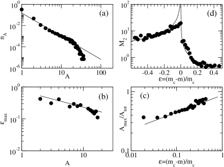
FIG. 4.: The critical exponents at $\tau_{ff}$: $\tau$ (a), $\sigma$ (b) , $\beta$ (c) and $\gamma$ (d). In (a) we plot the number of clusters per particle, $n(A)$, as a function of the mass number $A$ and its best fit (full line). In (b), the value of $\epsilon_{max}$ (defined in the text), is plotted against the mass number $A$ and its best fit (full line). The slope gives the value of $\sigma$. In (c) we plot the mass of the biggest fragment normalized to the size of the system ($A_{max}/A_{tot}$) as a function of $\epsilon=\frac{m_{c}-m}{m_{c}}$ and its fit giving the value of $\beta$. In (d) we plot the $M_{2}$ as a function of $\epsilon$ and the curve with the value of $\gamma$ obtained in the fitting procedure (full line).

We have seen in the previous section that the argument of the scaling function, $z$, can be expressed in terms of $\sigma$ via equation (7). Taking into account that $f(z)$ has a single maximum, we can calculate $\sigma$ in terms of the multiplicity by looking for the value of $\epsilon$ ($\epsilon_{max}$) that maximizes the production of clusters of a given size $A$:

$$n_{A}^{max}(\epsilon_{max})=q_{0}A^{-\tau}f(z_{max}),$$ (13)

where the argument of $f$ is $z_{max}=A^{\sigma}\epsilon_{max}$. This can be rewritten as:

$$\epsilon_{max}=z_{max}A^{-\sigma}$$ (14)

Therefore, by plotting $\epsilon_{max}$, as a function of $A$ we get $\sigma$ and $z_{max}$ [10, 20]. The results obtained are $\sigma=0.51\pm 0.15$ for $\tau_{ff}$ and $\sigma=0.64\pm 0.18$ for $\tau_{a}$, and they are plotted in figures 4(b) and 5(b) respectively. Although the values of $\sigma$ at time of fragment formation and at fragmentation time do not agree as well as $\tau$, they do agree when error bars are considered.

We calculate then the $\beta$ exponent related to behavior of the order parameter, which in our case is the biggest fragment mass ($A_{max}$). The behavior in the limit $\epsilon\rightarrow 0$ in an infinite system is given by:

$$(A_{\max}/A_{tot})\propto\epsilon^{\beta},\;\epsilon<0,$$ (15)

where $A_{max}$ is the average mass of the biggest fragment at a given multiplicity, $A_{tot}$ is the mass of the system and $\epsilon$ the distance to the critical point as defined above. In finite systems, 15 is valid in an intermediate region of $\epsilon$ where finite size effects are negligible. The relations $(A_{max}/A_{tot})\hskip 5.69046ptvs\hskip 5.69046pt\epsilon$ are displayed in figures 4(c) for $\tau_{ff}$ and 5(c) for $\tau_{a}$. The obtained values of $\beta$ are $0.29\pm 0.08$ and $0.28\pm 0.13$ respectively. These values are very close to $0.31$, which is the one corresponding to liquid-gas transition (3D-Ising Universality class ), and far from the percolation one (0.45). However, we believe that the smallness of the system is responsible of the large errors in $\beta$ and of a possible sub-valuation of the exponent, as was noticed in [22].

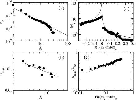
FIG. 5.: The same plot that in figure (4) but for asymptotic time $\tau_{a}$

.

As we have shown in equation (11), the behavior of $M_{2}$ near the critical point can be described in terms of the critical exponent $\gamma$. However the divergence predicted in this equation for the limit $\epsilon\rightarrow 0$, is valid for an infinite system. For a finite system, we have to find an intermediate region of $\epsilon$ where $M_{2}\propto\epsilon^{\gamma}$ (In this calculation, the biggest fragment of each event is removed when the multiplicity is below $m_{c}$). The procedure used to determine $\gamma$ is the following [10]: first, we take a value of $m_{c}$ from the range given by $NVM$, $M_{2}$ and the best fitted mass spectrum. Then we determine two ranges of fitting boundaries, one for the gas region ($\epsilon<0$, [$\epsilon_{g}^{min}:\epsilon_{g}^{max}]$) and the other for the liquid region $(\epsilon>0,[\epsilon_{l}^{min}:\epsilon_{l}^{max}])$. In each one of these regions, we fit the $M_{2}(m)$ to a power law, saving the exponents $\gamma_{g}$ and $\gamma_{l}$, and their corresponding $\chi_{g}^{2}$ and $\chi_{l}^{2}$ for the gas and the liquid regions respectively. For each value of $m_{c}$ we make several fitting procedures in a wide range of $\epsilon$, choosing those exponents ($\gamma_{g}$ and $\gamma_{l}$) that fulfil two conditions: first, the values should match each other within the error bars given by the fitting routine, and second, the $\chi^{2}$ of the fits should lie in the lowest twenty percent of the distribution. The values that satisfy these criteria were histogrammed and the average value ($<\gamma>$) and the variance ($\sigma_{\gamma}$) were obtained from the corresponding distribution . At $\tau_{ff}$ we got $\gamma=0.77\pm 0.25$ and at $\tau_{a},$ $\gamma=0.72\pm 0.33$. The results obtained are displayed in figures 4(d) and 5(d) for $\tau_{ff}$ and $\tau_{a}$ respectively. We can see that the value of $\gamma$ is smaller than the one expected for a liquid-gas phase transition, although far away from the percolation value (see table I).

In Table 1 we can see the values of the critical exponents calculated at time of fragment formation ($\tau_{ff}$) and at asymptotic times ($\tau_{a}$). Moreover, the values of these exponents for two different universality classes, 3D-Ising and Percolation, are also presented. It is clear from this table that:

1 - The time evolution after fragmentation time does not alter significatively the values of the critical exponents, i.e. the exponents obtained from asymptotic fragments distributions properly characterize the fragmentation process.

2 - The exponents are closer to the liquid-gas universality class than to the percolation one. However, despite the strong evidence arisen in the previous subsection (see Fig. 3), we can not be conclusive about the critical behavior of the drop: the error bars in $\sigma$ avoid us to discern if the transition could be cast in some of the universality clasess presented; the value of $\beta$ is closer to 3D-Ising but it could be sub-valuated due to the smallness of the system, and finally $\gamma$ shows a value close to 3D-Ising, but a little bit lower than the expected value for this universality class.

We think that two main features of the studied system should be taken into account in order to analyze the obtained results. First its finite size, that smoothes any signal of the possible phase transition and, consequently, induce quite large error bars for the calculated exponents. Second, even a certain degree of equilibration can be achieved at $\tau_{ff}$, non-equilibrium effects could still be noticeable (see [cherison]) and be responsible of the disagreement between the obtained $\gamma$ exponent and the expected value from the 3D-Ising Universality class.

TABLE I.: Critical exponents calculated at fragmentation and asymptotic time, and the corresponding to the 3DIsing (liquid-gas) and Percolation universality class [20,21]

. Exponents $\tau_{ff}$ $\tau_{a}$ 3D-Ising Percolation $\tau$ $2.18\pm 0.03$ $2.18\pm 0.03$ 2.21 2.18 $\sigma$ $0.51\pm 0.15$ $0.64\pm 0.18$ 0.64 0.45 $\beta$ $0.29\pm 0.08$ $0.28\pm 0.13$ 0.33 0.41 $\gamma$ $0.77\pm 0.25$ $0.72\pm 0.33$ 1.23 1.82

IV Conclusions

In conclusion, we have calculated different signals of critical behavior at fragmentation time as well as at asymptotic time. We have found that the dynamical evolution that follows the fragmentation process does not change the system criticallity features, i.e., the critical exponents values calculated at time of fragment formation. In this way, this work shows that it is possible to get the critical exponents that describes the physics involved in the fragmentation process from the mass distribution obtained experimentally. On the other hand, we can not assure than the process under study can be cast into the 3D-Ising universality class nor into the percolation one. In particular, the $\gamma$ exponent is far too low from the corresponding value for 3D-Ising class. This might suggest that non-equilibrium effects play a crucial role at time of fragment formation. Actually, at this time the system is in expansion and the collective motion is noticeable for excitation energies near the critical point, as was observed in the caloric curve of Ref.[17].

We acknowledge partial financial support from UBA grant EX139. P.B and A.C are fellows of the CONICET. C.O.D. is a member of the Carrera del Investigador (CONICET)

REFERENCES

- [1] A.S.Hirsch, A.Bujak, J.E.Finn, L.J.Gutay, R.W.Minich, N.T.Porile, R.P.Scharenberg, B.C. Stringfellow and F.Turkot, Phys.Rev.C 29, 508 (1984).
- [2] M. L. Gilkes et al., Phis. Rev.Lett. 73, 271 (1994).
- [3] M. Belkacem, V. Latora and A. Bonasera, Phys. Rev. C 52, 271 (1995).
- [4] A. Bonasera, M. Bruno, C. O. Dorso and P. F. Mastinu, La Rivista del Nuovo Cimento 23, 2 (2000)
- [5] J. A. Lopez and C. O. Dorso, ”Phase Transformation in Nuclear Matter”, World Scientific, (2000).
- [6] F. Gulminelli and P. Chomaz, Phys. Rev. Lett. 82, 1402 (1999); J.M. Carmona, N. Michel, J. Richert, and P.Wagner, Phys. Rev. C,61 037304 (2000).
- [7] J.B. Elliott, M.L.Gilkes, J.A.Hauger, A.S.Hirsch, E.Hjort, N.T.Porile, R.P.Scharenberg, B.K.Srivastava, M.L.Tincknell and P.G.Warren , Phys. Rev. C 55,1319 (1997).
- [8] J. B. Natowitz et al., Phys. Rev. C 65 (2002) 034618.
- [9] M. D’Agostino et.al. Nucl. Phys. A 650, 329 (1999).
- [10] J. B. Elliott et al., Phys. Rev. C 62 (2000) 064603.
- [11] M. Kleine Berkenbusch, W. Bauer et al., Phys.Rev.Lett. 88 (2002) 022701.
- [12] C. O. Dorso and J. Randrup, Phys. Lett. B 301, 328 (1993).
- [13] A. Strachan and C. O. Dorso, Phys. Rev. C 56,995 (1997).
- [14] A. Strachan and C. O. Dorso, Phys. Rev. C 59,285 (1999).
- [15] A. Chernomoretz, C. O. Dorso and J. A. Lopez, Phys. Rev. C 64,044605 (2001).
- [16] C. O. Dorso and J. Aichelin, Phys. Lett. B 345, 197 (1995).
- [17] A. Chernomoretz, M. Ison, S. Ortiz and C. O. Dorso, Phys. Rev. C 64,024606 (2001).
- [18] F. Gulminelli, Ph. Chomaz, M. Bruno and M. D’Agostino, Phys.Rev. C 65 (2002) 051601.
- [19] D. Stauffer and A. Aharoni, “Introduction to Percolation Theory”, 2nd edition, (Taylor and Francis, London, 1992).
- [20] H. Nakanishi and H. E. Stanley, Phys. Rev. B 22, 2466 (1980).
- [21] C. O. Dorso, V. C. Latora and A. Bonasera , Phys. Rev. C, 60, 034606 (1999).
- [22] J.B. Elliott, M.L.Gilkes, J.A.Hauger, A.S.Hirsch, E.Hjort, N.T.Porile, R.P.Scharenberg, B.K.Srivastava, M.L.Tincknell and P.G.Warren , PRC 49,3185 (1994).
- [23] A. Chernomoretz, P.Balenzuela and C.O.Dorso, preprint arXiv:nucl-th/0203050.