Renormalization Group Equation for Low Momentum Effective Nuclear Interactions

Abstract

We consider two nonperturbative methods originally used to derive shell model effective interactions in nuclei. These methods have been applied to the two nucleon sector to obtain an energy independent effective interaction $V_{\text{low k}}$, which preserves the low momentum half-on-shell $T$ matrix and the deuteron pole, with a sharp cutoff imposed on all intermediate state momenta. We show that $V_{\text{low k}}$ scales with the cutoff precisely as one expects from renormalization group arguments. This result is a step towards reformulating traditional model space many-body calculations in the language of effective field theories and the renormalization group. The numerical scaling properties of $V_{\text{low k}}$ are observed to be in excellent agreement with our exact renormalization group equation.

PACS: 21.30.Fe; 13.75.Cs; 11.10.Hi; 03.65.Nk
Keywords: Nucleon-Nucleon Interactions; Effective Interactions; Renormalization Group; Scattering Theory

1 Introduction

There has been much work over the past decade applying the techniques of effective field theory (EFT) and the renormalization group (RG) to low energy nuclear systems such as the nucleon-nucleon force, finite nuclei, and nuclear matter [1]. Conventional nuclear force models such as the Paris, Bonn, and Argonne potentials incorporate the same asymptotic tail generated by one pion exchange, as the long wavelength structure of the interaction is unambiguously resolved from fits to low energy phase shifts and deuteron properties. The short wavelength part of the interaction is then generated by assuming a specific dynamical model based on heavy meson exchanges, combined with phenomenological treatments at very small distances. Such approaches are necessarily model dependent, as the low energy two-nucleon properties are insufficient to resolve the short distance structure. Such model dependence often appears in many-body calculations, e.g. the Coester band in nuclear matter, when highly virtual nucleons probe the short distance structure of the interaction. The EFT approach eliminates the unsatisfactory model dependence of conventional force models and provides an effective description that is consistent with the low energy symmetries of the underlying strong interactions (QCD). This is accomplished by keeping only nucleons and pions as explicit degrees of freedom, as dictated by the spontaneously broken chiral symmetry of QCD. All other heavy mesons and nucleon resonances are considered to be integrated out of the theory, their effects contained inside the renormalized pion exchange and scale dependent coupling constants that multiply model independent delta functions and their derivatives [2]. No underlying dynamics are assumed for the heavy mesons and nucleon resonances, as they simply cannot be resolved from low energy data. Since RG decimations generate all possible interactions consistent with the symmetries of the underlying theory, it is sufficient to consider all interactions mandated by chiral symmetry and then tune the couplings to the low energy data. Power counting arguments are then used to truncate the number of couplings that need to be fit to experiment, thus endowing the EFT with predictive power and the ability to estimate errors resulting from the truncation. Moreover, the breakdown of the EFT at a given scale signals the presence of new relevant degrees of freedom that must be considered explicitly to properly describe phenomena at that scale.

Similar concepts of integrating out the high energy modes have long been used to derive effective interactions in nuclei within a truncated model space, e.g. the sd-shell for the two valence nucleons in ¹⁸O. Starting from the vacuum two-body force in the full many-body Hilbert space, one can construct an effective theory for the low-lying excitations provided the effective interaction encodes the effects of the integrated high energy modes. Although the traditional model space methods apparently share similarities to the modern RG-EFT approaches, these have not been exploited until recently [3, 4, 5, 6] and not sufficiently in any realistic nuclear many-body calculation. In the traditional approaches, there has been little success in predicting how the effective interaction changes with the model space size. In RG language, no beta functions have been derived that would allow one to calculate an effective interaction in one convenient choice of model space, and then evolve the effective theory to any other scale by following the flow of the beta function. Moreover, one could push the analogy with EFT further by projecting the effective interaction onto a few leading operators, with the ability to reliably estimate the errors on calculated nuclear spectra resulting from this truncation. Therefore, it is of greatest interest to address the issue of calculating beta functions within the framework of model space effective interaction methods and to exploit these powerful similarities with the RG-EFT approach.

Two well known methods for deriving energy independent model space interactions are the Kuo-Lee-Ratcliff (KLR) folded diagram theory [7] and the related similarity transformation method of Lee and Suzuki (LS) [8]. The authors have applied these methods to the nucleon-nucleon problem in vacuum where the model space was taken to be plane wave states with relative momenta $k<\Lambda$. The resulting unique low momentum potential $V_{\text{low k}}$ preserves the deuteron binding energy and the low energy half-on-shell $T$ matrix, but with all intermediate state summations cut off at $\Lambda$ [3]. In this paper, we restrict our analysis to the two-body problem in free space. We show that the model space interaction $V_{\text{low k}}$ scales with $\Lambda$ in the same way one would expect from a exact RG treatment of the scattering problem. In this way, we show that the methods originally used to derive model space interactions in nuclei can be interpreted in modern language as renormalization group decimations, at least for two-body correlations in the nucleus. This work is a step towards reformulating traditional nuclear many-body methods in a manner consistent with the more systematic and controlled RG-EFT approaches. To the best of our knowledge, this is a genuinely new result as previous RG studies have dealt with energy dependent effective potentials [9]. It is also the first RG flow study of realistic nucleon-nucleon interactions. From a practical perspective, it is simpler to use energy independent effective interactions in many-body calculations, as one does not have to recalculate the interaction vertex depending on the energy variable of the propagator it is linked to in a particular diagram.

2 RG from half-on-shell $T$ Matrix Equivalence

Let us begin with a RG treatment of the scattering problem. Working in a given partial wave we denote the bare (Bonn, Paris, Argonne, etc.) two-body potential as $V_{\text{NN}}$, although the following developments are general and apply to any nonrelativistic scattering problem. Employing principle value propagators we have the half-on-shell (HOS) $T$ matrix equation [10]

$$T(k^{\prime},k;k^{2})=V_{\text{NN}}(k^{\prime},k)+\frac{2}{\pi}\,\mathcal{P}\int_{0}^{\infty}\frac{V_{\text{NN}}(k^{\prime},p)\,T(p,k;k^{2})}{k^{2}-p^{2}}\,p^{2}dp.$$ (1)

In a RG treatment of two-body scattering, we impose a cutoff $\Lambda$ on all the loop integrals in the $T$ matrix equation and replace the bare $V_{\text{NN}}$ with an effective potential $V_{\text{low k}}$. The effective potential is independent of the scattering energy and is allowed to depend on $\Lambda$ so that $T(k^{\prime},k;k^{2})$ for $k,k^{\prime}<\Lambda$ is preserved. Clearly this is sufficient to ensure that low energy observables, which are fully on-shell quantities are independent of $\Lambda$. Explicitly, we have

$$T(k^{\prime},k;k^{2})=V_{\text{low k}}(k^{\prime},k)+\frac{2}{\pi}\,\mathcal{P}\int_{0}^{\Lambda}\frac{V_{\text{low k}}(k^{\prime},p)\,T(p,k;k^{2})}{k^{2}-p^{2}}\,p^{2}dp.$$ (2)

By construction, the low momentum HOS $T$ matrices calculated from Eq. (1) and Eq. (2) are identical. Consequently, the low momentum components of the low energy scattering states are preserved. We denote the standing wave scattering states of the effective theory by $|\chi_{k}\rangle$, which can be written in the standard fashion as

$$|\chi_{k}\rangle=|k\rangle+\frac{2}{\pi}\,\mathcal{P}\int_{0}^{\Lambda}\,p^{2}dp\,\frac{1}{k^{2}-p^{2}}\,T(p,k;k^{2})\,|p\rangle.$$ (3)

We therefore take $dT(k^{\prime},k;k^{2})/d\Lambda=0$ in Eq. (2) to obtain a flow equation for $V_{\text{low k}}$

$$\int_{0}^{\Lambda}\frac{dV_{\text{low k}}(k^{\prime},p)}{d\Lambda}\>\chi_{k}(p)\>p^{2}dp=\frac{2}{\pi}\frac{V_{\text{low k}}(k^{\prime},\Lambda)\,T(\Lambda,k;k^{2})}{1-(k/\Lambda)^{2}}.$$ (4)

By writing $T(\Lambda,k;k^{2})=\langle\Lambda|V_{\text{low k}}|\chi_{k}\rangle$ and using the completeness of the scattering states in the model space , we obtain

$$\frac{d}{d\Lambda}V_{\text{low k}}(k^{\prime},p^{\prime}) =\frac{2}{\pi}\,V_{\text{low k}}(k^{\prime},\Lambda)\int_{0}^{\Lambda}\frac{\langle\Lambda|V_{\text{low k}}|\chi_{k}\rangle\>\langle\widetilde{\chi}_{k}|p^{\prime}\rangle}{1-(k/\Lambda)^{2}}\>k^{2}dk$$

$$=\frac{2}{\pi}\,\Lambda^{2}\,V_{\text{low k}}(k^{\prime},\Lambda)\int_{0}^{\Lambda}V_{\text{low k}}(\Lambda,p)\>\mathcal{G}(p,p^{\prime};\Lambda^{2})\>p^{2}dp.$$ (5)

where $\mathcal{G}$ denotes the interacting Green’s function in the effective theory. Writing the interacting Green’s function in terms of the $T$ matrix in the low momentum sector we obtain the exact RG equation

$$\frac{d}{d\Lambda}V_{\text{low k}}(k^{\prime},k)=\frac{2}{\pi}\frac{V_{\text{low k}}(k^{\prime},\Lambda)\>T(\Lambda,k;\Lambda^{2})}{1-(k/\Lambda)^{2}}.$$ (6)

The derivation of Eqs. (5,6) is similar to the work of Birse et al. [9], although they consider the fully off-shell $T$ matrix and an energy dependent effective potential $V_{\text{eff}}$. The RG equation of Birse et al. is exact to second order in $V_{\text{eff}}$. It reads

$$\frac{d}{d\Lambda}V_{\text{eff}}(k^{\prime},k;p^{2})=\frac{2}{\pi}\frac{V_{\text{eff}}(k^{\prime},\Lambda;p^{2})\>V_{\text{eff}}(\Lambda,k;p^{2})}{1-(p/\Lambda)^{2}},$$ (7)

where $p^{2}$ denotes the scattering energy.

Our RG treatment is based on HOS $T$ matrix preservation, as this is the minimally off-shell quantity needed to preserve the low energy phase shifts as well as the low momentum components of the wave functions, while allowing one to consider an energy independent effective interaction. Our exact RG equation for energy independent effective interactions, Eq. (6), agrees with the result of Birse et al. [9] at the one-loop level. As we shall see below, the starting point of energy independent effective interaction methods is the above off-shell effective potential, and the energy dependence is subsequently traded for momentum dependence. This procedure is similar to using the equations of motion in many-body physics to trade the energy dependence in favor of a more complicated quasiparticle dispersion relation.

3 RG from the KLR Folded Diagram Corrections

In the previous section, we obtained the RG equation for $V_{\text{low k}}$, Eq. (5), from $T$ matrix equivalence alone. We now derive the same equation using the Kuo-Lee-Ratcliff (KLR) folded diagram technique, originally designed for constructing energy independent model space interactions in shell model applications [7]. First, we define an energy dependent vertex function called the $\widehat{Q}$ box, that is irreducible with respect to cutting intermediate low momentum propagators. The $\widehat{Q}$ box resums the effects of the high momentum modes we wish to integrate out of the theory,

$$\widehat{Q}(k^{\prime},k;\omega)=V_{\text{NN}}(k^{\prime},k)+\frac{2}{\pi}\,\mathcal{P}\int_{\Lambda}^{\infty}\frac{V_{\text{NN}}(k^{\prime},p)\,\widehat{Q}(p,k;\omega)}{\omega-p^{2}}\,p^{2}dp.$$ (8)

It is the same energy dependent effective potential studied by Weinberg in the context of chiral lagrangians [11] and by Birse et al. for the purpose of an RG treatment of two-body scattering [9]. In terms of the $\widehat{Q}$ box the HOS $T$ matrix reads

$$T(k^{\prime},k;k^{2})=\widehat{Q}(k^{\prime},k;k^{2})+\frac{2}{\pi}\,\mathcal{P}\int_{0}^{\Lambda}\frac{\widehat{Q}(k^{\prime},p;k^{2})\,T(p,k;k^{2})}{k^{2}-p^{2}}\,p^{2}dp.$$ (9)

The original literature develops KLR folded diagrams using time-ordered perturbation theory for systems with degenerate unperturbed model space spectra. In this framework, the folded diagrams can be viewed as correction terms one must add, if one factorizes the nested time-integrals one finds in time-ordered perturbation theory for Dyson equations. For the present work, it is much easier to understand the meaning of folded diagrams in the time-independent framework. Iterating Eq. (9), it is clear that all $\widehat{Q}$ box vertices are fully off-shell with the exception of the final $\widehat{Q}$ box in each term. The folded diagrams are correction terms one must add, if all $\widehat{Q}$ boxes are evaluated right-side on-shell in the Dyson equation. In order to see how this works, the second order $\widehat{Q}$ box contribution in Eq. (9) can be written as

$$\int_{p}\frac{\widehat{Q}(k^{\prime},p;k^{2})\,\widehat{Q}(p,k;k^{2})}{k^{2}-p^{2}}=\int_{p}\frac{\widehat{Q}(k^{\prime},p;p^{2})\,\widehat{Q}(p,k;k^{2})}{k^{2}-p^{2}}\>+\>\mathcal{V}^{1-\text{fold}}(k^{\prime},k),$$ (10)

where $\mathcal{V}^{\text{1-fold}}$ denotes the “one-fold correction” and $\int_{p}\equiv 2/\pi\int_{0}^{\Lambda}p^{2}dp$ is shorthand for the model space principle value measure. With the expression for $\mathcal{V}^{\text{1-fold}}$, we write the KLR folded diagram series for $V_{\text{low k}}$ to one-fold, or equivalently to second order in the $\widehat{Q}$ box as

$$V_{\text{low k}}(k^{\prime},k)=\widehat{Q}(k^{\prime},k;k^{2})\\ +\int_{p}\frac{\widehat{Q}(k^{\prime},p;k^{2})-\widehat{Q}(k^{\prime},p;p^{2})}{k^{2}-p^{2}}\,\widehat{Q}(p,k;k^{2})\>+\mathcal{O}(\widehat{Q}^{3}).$$ (11)

Analogously, the two-fold correction to the KLR $V_{\text{low k}}$ is obtained by considering the $\mathcal{O}(\widehat{Q}^{3})$ contribution of Eq. (9) and correcting for putting all $\widehat{Q}$ boxes right-side on-shell. The resulting two-fold correction is given by

$$\mathcal{V}^{2-\text{fold}}(k^{\prime},k)=\iint\limits_{p,p^{\prime}}\frac{\widehat{Q}(k^{\prime},p^{\prime};k^{2})-\widehat{Q}(k^{\prime},p^{\prime};p^{\prime 2})}{(k^{2}-p^{\prime 2})(k^{2}-p^{2})}\,\widehat{Q}(p^{\prime},p;k^{2})\,\widehat{Q}(p,k;k^{2})\\[2.84526pt] -\iint\limits_{p,p^{\prime}}\frac{\widehat{Q}(k^{\prime},p^{\prime};p^{2})-\widehat{Q}(k^{\prime},p^{\prime};p^{\prime 2})}{(p^{2}-p^{\prime 2})(k^{2}-p^{2})}\,\widehat{Q}(p^{\prime},p;p^{2})\,\widehat{Q}(p,k;k^{2}).$$ (12)

Proceeding in a similar manner for the higher order terms in the Dyson equation, one can write the KLR expression for $V_{\text{low k}}$ as

$$V_{\text{low k}}\equiv\widehat{Q}+\mathcal{V}^{1-\text{fold}}+\mathcal{V}^{2-\text{fold}}+\mathcal{V}^{3-\text{fold}}+\ldots\>.$$ (13)

Having motivated the KLR folded diagram series, we now derive a flow equation that tells us how the KLR $V_{\text{low k}}$ changes as one changes the scale $\Lambda$. The first step is to notice that the $\widehat{Q}$ box, and hence the KLR series, obeys the semi-group composition law. We can therefore perform the decimation to $\Lambda$ in one step using the bare $V_{\text{NN}}$ as input, or equivalently we can integrate out recursively in small steps; each subsequent step in the decimation uses the $V_{\text{low k}}$ of the previous step as input. Let us therefore start with the KLR $V_{\text{low k}}$ at a cutoff $\Lambda$, and ask how $V_{\text{low k}}$ changes as we integrate out the states lying in the momentum shell $\Lambda-\delta\Lambda<k<\Lambda$. Referring to the definition of the $\widehat{Q}$ box, Eq. (8), it is clear that each intermediate loop integration is $\mathcal{O}(\delta\Lambda)$. Therefore, we have for $\widehat{Q}^{\Lambda-\delta\Lambda}$

$$\widehat{Q}^{\Lambda-\delta\Lambda}(k^{\prime},k;p^{2})=V^{\Lambda}_{\text{low k}}(k^{\prime},k)\\ -\delta\Lambda\,\frac{2}{\pi}\,\frac{V^{\Lambda}_{\text{low k}}(k^{\prime},\Lambda)\,V^{\Lambda}_{\text{low k}}(\Lambda,k)}{1-(p/\Lambda)^{2}}\,+\mathcal{O}(\delta\Lambda^{2}),$$ (14)

where the superscript denotes at which step the low momentum potential and the $\widehat{Q}$ box are evaluated. Although we have given explicit formulas only up to two folds, this will be sufficient to derive the flow equation. The generalization to all orders in $V_{\text{low k}}$ can be found in the appendix, where energy independent effective interactions are related to the spectral representation of the HOS $T$ matrix. We insert the expression for the $\widehat{Q}^{\Lambda-\delta\Lambda}$ box, Eq. (14), into the KLR folded diagram series, Eq. (13), and find

$$\delta V_{\text{low k}}(k^{\prime},k)=\delta\Lambda\,\frac{2}{\pi}\,\frac{V^{\Lambda}_{\text{low k}}(k^{\prime},\Lambda)}{1-(k/\Lambda)^{2}}\,\biggl{\{}\,V^{\Lambda}_{\text{low k}}(\Lambda,k)+\int_{p}\frac{V^{\Lambda}_{\text{low k}}(\Lambda,p)\,V^{\Lambda}_{\text{low k}}(p,k)}{\Lambda^{2}-p^{2}}\\[2.84526pt] +\iint\limits_{p,p^{\prime}}\frac{V^{\Lambda}_{\text{low k}}(\Lambda,p)\,V^{\Lambda}_{\text{low k}}(p,p^{\prime})\,V^{\Lambda}_{\text{low k}}(p^{\prime},\Lambda)}{(\Lambda^{2}-p^{2})\,(\Lambda^{2}-p^{\prime 2})}+\mathcal{O}\bigl{(}(V^{\Lambda}_{\text{low k}})^{4}\bigr{)}\,\biggr{\}}\,+\mathcal{O}(\delta\Lambda^{2}).$$ (15)

Passing to the limit $\delta\Lambda\to 0$, we sum the flow equation and obtain

$$\frac{d}{d\Lambda}V_{\text{low k}}(k^{\prime},k)=\frac{2}{\pi}\,\frac{V_{\text{low k}}(k^{\prime},\Lambda)\,T(\Lambda,k;\Lambda^{2})}{1-(k/\Lambda)^{2}}.$$ (16)

This proves that the KLR $V_{\text{low k}}$ obeys the same scaling equation one obtains using RG arguments based on $T$ matrix preservation alone. It does not come as a surprise, as it has been shown diagrammatically that the KLR effective theory preserves the low momentum HOS $T$ matrix of the input bare potential [12]. Nevertheless, we have here derived the same flow equation in a manner that makes no reference to $T$ matrix preservation. It may be regarded as an algebraic proof that the folded diagram series preserves the HOS $T$ matrix. This firmly establishes that the KLR folded diagram theory is equivalent to a RG decimation, at least for the two-nucleon sector.

4 RG from the LS Similarity Transformation

It is easy to see how the folded diagram series is constructed. The n-folded diagram is the correction terms one must add, if one evaluates all soft-mode irreducible vertex functions right-side on-shell in the term of $\mathcal{O}(\widehat{Q}^{n+1})$ of any Dyson equation. As we have seen above, the expression for the two-fold contribution is already rather cumbersome. The Lee-Suzuki scheme is an iterative method that is often used in the calculation of shell model effective interactions [8]. It has been shown to converge to the folded diagram series [7]. While the LS method does not lend itself to a simple diagrammatic interpretation, we show how the same flow equation evolves from the iteration scheme, as this provides a check to our RG equation. The details of the LS method may be found in [8]. The defining equations of the LS iteration are given by

$$H_{\text{low k}}^{(1)} =PH_{0}P+\widehat{Q}(\omega)\arrowvert_{\omega=0}$$ (17)

$$H_{\text{low k}}^{(2)} =\frac{1}{1-\widehat{Q}^{(1)}}\,H_{\text{low k}}^{(1)}$$ (18)

$$H_{\text{low k}}^{(3)} =\frac{1}{1-\widehat{Q}^{(1)}-\widehat{Q}^{(2)}\,H_{\text{low k}}^{(2)}}\,H_{\text{low k}}^{(1)}$$ (19)

$$\hskip 5.69046pt\vdots$$

$$H_{\text{low k}}^{(n)} =\frac{1}{1-\widehat{Q}^{(1)}-\widehat{Q}^{(2)}\,H_{\text{low k}}^{(n-1)}-\ldots-\widehat{Q}^{(n-1)}\,H_{\text{low k}}^{(2)}\,\cdots\,H_{\text{low k}}^{(n-1)}}\,H_{\text{low k}}^{(1)}$$ (20)

$$\widehat{Q}^{(n)} \equiv\frac{1}{n!}\,\frac{d^{n}}{d\omega^{n}}\widehat{Q}(\omega)\arrowvert_{\omega=0}.$$ (21)

As for the KLR folded diagram theory, we derive the flow equation for $V_{\text{low k}}$ directly from the LS equations by invoking the semi-group composition law and considering an infinitesimal decimation from $\Lambda$ to $\Lambda-\delta\Lambda$. Suppose we have solved the LS equations for $V^{\Lambda}_{\text{low k}}=H^{\Lambda}_{\text{low k}}-PH_{0}P$ at some value of $\Lambda$, where $P$ denotes the projection operator on the model space. Keeping terms to first order in $\delta\Lambda$, we find

$$\widehat{Q}^{\Lambda-\delta\Lambda}(p^{\prime},p;0) =V^{\Lambda}_{\text{low k}}(p^{\prime},p)-\delta\Lambda\,\frac{2}{\pi}\,V^{\Lambda}_{\text{low k}}(p^{\prime},\Lambda)\,V^{\Lambda}_{\text{low k}}(\Lambda,p)$$ (22)

$$\widehat{Q}^{(n)\Lambda-\delta\Lambda}(p^{\prime},p) =-\delta\Lambda\,\frac{2}{\pi}\,\frac{V^{\Lambda}_{\text{low k}}(p^{\prime},\Lambda)\,V^{\Lambda}_{\text{low k}}(\Lambda,p)}{\Lambda^{2n}}.$$ (23)

Substituting the above expressions into the defining LS equations and keeping terms only to $\mathcal{O}(\delta\Lambda)$, one obtains

$$H^{\Lambda-\delta\Lambda}_{\text{low k}}\,(p^{\prime},p)=H^{\Lambda}_{\text{low k}}(p^{\prime},p)-\delta\Lambda\>V^{\Lambda}_{\text{low k}}(p^{\prime},\Lambda)\int_{k}V^{\Lambda}_{\text{low k}}(\Lambda,k)\>\mathcal{S}(k,p),$$ (24)

where

$$\mathcal{S}(k,p)=\frac{1}{k^{2}}\>\delta(k-p)+\int_{q}\frac{H^{\Lambda}_{\text{low k}}(k,q)}{\Lambda^{2}}\>\mathcal{S}(q,p).$$ (25)

The expression for $\mathcal{S}$ can be summed to give the interacting Green’s function $\mathcal{S}(k,p)=\Lambda^{2}\,\mathcal{G}(k,p;\Lambda^{2})$ of the effective theory. In the limit $\delta\Lambda\to 0$, we thus obtain the following RG equation directly from the Lee-Suzuki equations

$$\frac{d}{d\Lambda}V_{\text{low k}}(p^{\prime},p) =\frac{2}{\pi}\,\Lambda^{2}\>V_{\text{low k}}(p^{\prime},\Lambda)\int_{0}^{\Lambda}V_{\text{low k}}(\Lambda,k)\>\mathcal{G}(k,p;\Lambda^{2})\>k^{2}\,dk$$ (26)

$$=\frac{2}{\pi}\frac{V_{\text{low k}}(p^{\prime},\Lambda)\>T(\Lambda,p;\Lambda^{2})}{1-(p/\Lambda)^{2}}.$$ (27)

Thus, we obtain the same scaling equation from the LS and KLR effective interaction methods as we obtain from RG arguments based on $T$ matrix equivalence. Hence, it is clear that the traditional model space methods of nuclear structure can be employed to perform RG decimations in the two nucleon sector.

5 Numerical Comparison of the Beta Function

We have provided four different derivations of the same RG equation, which describes the scaling of the effective potential $V_{\text{low k}}$ with $\Lambda$ so that the low energy observables are preserved by the effective theory. For completeness, we provide numerical confirmation of the RG equation in this section. Starting from a model of the nuclear force such as the Paris, Bonn-A, Argonne V-18, or Idaho-A potential, we have integrated out the model dependent high momentum modes of the theory using the KLR/LS methods to obtain an effective potential $V_{\text{low k}}$ [3]. The results of Bogner et al. are striking [3]: the high momentum modes of all studied potential models renormalize the low momentum interaction to a unique $V_{\text{low k}}$ for cutoffs $\Lambda\lesssim 2\;\text{fm}^{-1}$. The differences resulting from a chiral treatment of the 2$\pi$ exchange can be seen in the offdiagonal matrix elements of $V_{\text{low k}}$, and flow studies of the crucial s-wave matrix elements $V_{\text{low k}}(0,0)$ exhibit the relevant scales (pions, deuteron, and higher order tensor interactions) and for small model spaces are in excellent agreement with the power divergence subtraction scheme of Kaplan, Savage, and Wise [13]. For a discussion of all results see [3].

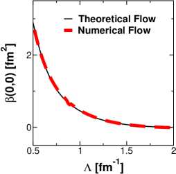
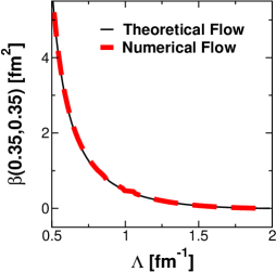
Figure 1: Comparison of numerical and theoretical “beta” functions in the ${}^{1}S_{0}$ partial wave calculated for the Paris potential.

Performing the calculation for a range of $\Lambda$ values, we calculate the numerical derivative $dV_{\text{low k}}/d\Lambda$ and compare it with the theoretical expression, Eq. (6). As in [3], the RG decimation is carried out with the iterative implementation of the LS method of Andreozzi [14]. Referring to Fig. (1), it is evident that the numerical derivative (numerical flow) is in excellent agreement with the exact “beta” function (theoretical flow) , $\beta\equiv\frac{d}{d\Lambda}V_{\text{low k}}$. Similar results are found for offdiagonal elements as well as other partial waves.

6 Conclusions

We have shown that model space effective interaction methods, such as the Kuo-Lee-Ratcliff folded diagram series and the Lee-Suzuki similarity transformation, scale with the model space boundary exactly as one would expect from RG arguments. We have derived the exact beta function for the energy independent, low momentum effective theory of two-body scattering. Our theoretical beta function is in perfect agreement with the numerical scaling behaviour of $V_{\text{low k}}$. This is a genuinely new result, as previous RG studies of two-body scattering consider energy dependent effective interactions [9].

In the RG formulation for effective theories, one can evolve the effective interaction according to the beta function given suitable initial conditions; in our case, the bare interaction for very large model spaces. Bogner et al. have performed such an RG decimation in the two-nucleon sector starting from realistic nucleon-nucleon potentials such as the Paris, Bonn-A, Argonne V-18, and Idaho-A interaction [3]. They found that the initially very different bare potentials renormalize to a unique $V_{\text{low k}}$ starting at a scale of $\Lambda\approx 2\;\text{fm}^{-1}$. Moreover, the authors have used the unique $V_{\text{low k}}$ directly in shell model calculations without first calculating the Brueckner $G$ matrix. They found very promising results using the same input $V_{\text{low k}}$ for two valence nuclei in different mass regions, and the results were nearly independent of the cutoff in the neighborhood of $2\;\text{fm}^{-1}$ [15]. Referring to Fig. (1), these results are consistent with the observation that the beta function is nearly zero in this region.

For energy dependent effective interactions, Birse et al. have studied the power counting imposed by means of a Wilson-Kadanoff rescaling. Their results have been very powerful in predicting only two well defined power-counting schemes for s-wave scattering [9] with short ranged forces. Their arguments can be extended to include long-range forces in a distorted wave basis [16], with qualitatively similar conclusions. We hope to generalize and apply the methods of Birse et al. to obtain a well defined power counting scheme for the energy independent $V_{\text{low k}}$. This is complicated since the “beta” function includes $V_{\text{low k}}$ to all orders.

In conclusion, the equivalence of model space effective interaction and RG methods in the two-body sector is a first step towards reformulating traditional effective interaction methods in a manner that fully exploits their similarities to RG-EFT methods, particularily their power to reliably estimate errors. The ultimate goal is to extend the RG arguments for $V_{\text{low k}}$ to the shell model effective interaction. At this point, it is restricted to two-particle correlations in the nucleus.

Appendix A Appendix

In this appendix, we provide the fourth and final derivation of the RG equation, Eq. (6), based on the spectral representation of the HOS $T$ matrix. Moreover, we show that HOS $T$ matrix preservation necessarily implies a non-hermitian energy independent $V_{\text{low k}}$. Without loss of generality, we employ a notation which suggests there are no bound states in the channel under consideration; bound states are easily handled by extending the completeness relation to include the relevant bound states in the summation.

We first prove that the energy independent $V_{\text{low k}}$ is necessarily non-hermitian, if it preserves the HOS $T$ matrix. We begin by assuming the contrary, i.e. we assume the energy independent $V_{\text{low k}}$ is hermitian and preserves the HOS $T$ matrix. We have

$$V_{\text{low k}}|\chi_{p}\rangle=\widehat{Q}(p^{2})|\chi_{p}\rangle.$$ (28)

Multiplying from the right with $\langle\chi_{p}|$ and integrating over $p$, the completeness of the model space eigenfunctions yields

$$V_{\text{low k}}(k^{\prime},k)=\int_{p}\>\langle k^{\prime}|\widehat{Q}(p^{2})|\chi_{p}\rangle\>\chi_{p}^{*}(k).$$ (29)

Expanding the $p^{2}$ dependence of the $\widehat{Q}$ box, one can use the equations of motion $(H_{0}+\widehat{Q}(p^{2}))|\chi_{p}\rangle=p^{2}|\chi_{p}\rangle$ to convert the $p^{2}$ dependence to $k^{\prime 2}$ dependence. For example, the $\mathcal{O}(p^{2})$ dependence is eliminated by letting $H_{0}$ act on $\langle k^{\prime}|$ and using Eq. (28) to trade the extra $\widehat{Q}$ for $V_{\text{low k}}$. It is clear from this simple example that the energy dependence is asymmetrically converted to $k^{\prime}$ dependence. Therefore, we conclude that the requirement of HOS $T$ matrix preservation necessarily implies a non hermitian $V_{\text{low k}}$. Technically speaking, this means that the completeness relation for the model space scattering states should be modified by replacing $\langle\chi_{p}|$ with the bi-orthogonal complement, $\langle\widetilde{\chi}_{p}|$.

Having shown that $V_{\text{low k}}$ is non-hermitian, we now derive the RG equation from the spectral representation of the HOS $T$ matrix. Inserting a complete set of low momentum plane waves between the $\widehat{Q}$ box and the low energy scattering wave function in Eq. (29), we obtain

$$V_{\text{lowk}}(k^{\prime},k)=\iint\limits_{p,p^{\prime}}\>\widehat{Q}(k^{\prime},p^{\prime};p^{2})\>\chi_{p}(p^{\prime})\>\widetilde{\chi}_{p}^{*}(k).$$ (30)

In terms of $T$ matrices, this can be written as

$$V_{\text{low k}}(k^{\prime},k)=T(k^{\prime},k;k^{2})+\int_{p}\>T(k^{\prime},p;p^{2})\>\frac{1}{p^{2}-k^{2}}\>T(p,k;p^{2}).$$ (31)

This is just a rearrangement of the spectral representation for the $T$ matrix. Differentiating Eq. (31) with respect to the cutoff we obtain the RG flow equation

$$\frac{dV_{\text{low k}}}{d\Lambda}(k^{\prime},k)= \,\frac{2}{\pi}\>V_{\text{low k}}(k^{\prime},\Lambda)\>\frac{\Lambda^{2}}{\Lambda^{2}-k^{2}}\>T(\Lambda,k;\Lambda^{2})$$

$$+\frac{2}{\pi}\>\int_{p}\>V_{\text{low k}}(k^{\prime},p)\>\frac{1}{\Lambda^{2}-p^{2}}\>T(p,\Lambda;\Lambda^{2})\>\frac{\Lambda^{2}}{\Lambda^{2}-k^{2}}\>T(\Lambda,k;\Lambda^{2})$$

$$+\int_{p}\>T(k^{\prime},p;p^{2})\>\frac{1}{p^{2}-k^{2}}\>\frac{dT(p,k;p^{2})}{d\Lambda}.$$ (32)

Now we show that the latter two terms in Eq. (32) cancel against each other. To this end, we write the left-side on-shell $T$ matrix in terms of the right-side on-shell one:

$$T(p,k;p^{2})=T(p,k;k^{2})+\int_{q}\>T(p,q;q^{2})\>\biggl{\{}\frac{1}{p^{2}-q^{2}}-\frac{1}{k^{2}-q^{2}}\biggr{\}}\>T(q,k;q^{2}).$$ (33)

By differentiating with respect to the cutoff, Eq. (33) yields

$$\frac{dT(p,k;p^{2})}{d\Lambda}=\frac{2}{\pi}\>T(p,\Lambda;\Lambda^{2})\>\biggl{\{}\frac{\Lambda^{2}}{p^{2}-\Lambda^{2}}-\frac{\Lambda^{2}}{k^{2}-\Lambda^{2}}\biggr{\}}\>T(\Lambda,k;\Lambda^{2})\\ +\int_{q}\>T(p,q;q^{2})\>\biggl{\{}\frac{1}{p^{2}-q^{2}}-\frac{1}{k^{2}-q^{2}}\biggr{\}}\>\frac{dT(q,k;q^{2})}{d\Lambda}.$$ (34)

We insert the integral equation for the right-side on-shell $T$ matrix, Eq. (2), into the last term of flow equation, Eq. (32). It results in the two terms

$$\int_{p}\>T(k^{\prime},p;p^{2})\>\frac{1}{p^{2}-k^{2}}\>\frac{dT(p,k;p^{2})}{d\Lambda}=\int_{p}\>V_{\text{low k}}(k^{\prime},p)\>\frac{1}{p^{2}-k^{2}}\>\frac{dT(p,k;p^{2})}{d\Lambda}$$

$$\hskip 28.45274pt+\iint\limits_{p,q}\>V_{\text{low k}}(k^{\prime},q)\>\frac{1}{p^{2}-q^{2}}\>T(q,p;p^{2})\>\frac{1}{p^{2}-k^{2}}\>\frac{dT(p,k;p^{2})}{d\Lambda}.$$ (35)

Finally, we combine Eq. (35) with the integral equation for $dT/d\Lambda$, Eq. (34), inserted into the $V_{\text{low k}}\,dT/d\Lambda$ term. Now the last two terms of the flow equation, Eq. (32), read

$$\frac{2}{\pi}\,\int_{p}\>V_{\text{low k}}(k^{\prime},p)\>\frac{1}{\Lambda^{2}-p^{2}}\>T(p,\Lambda;\Lambda^{2})\>\frac{\Lambda^{2}}{\Lambda^{2}-k^{2}}\>T(\Lambda,k;\Lambda^{2})$$

$$\;+\,\frac{2}{\pi}\,\int_{p}\>V_{\text{low k}}(k^{\prime},p)\>\frac{1}{p^{2}-k^{2}}\>T(p,\Lambda;\Lambda^{2})\>\biggl{\{}\frac{\Lambda^{2}}{p^{2}-\Lambda^{2}}-\frac{\Lambda^{2}}{k^{2}-\Lambda^{2}}\biggr{\}}\>T(\Lambda,k;\Lambda^{2})$$

$$\;\;\;+\iint\limits_{p,q}\>V_{\text{low k}}(k^{\prime},p)\>\frac{1}{p^{2}-k^{2}}\>T(p,q;q^{2})\>\biggl{\{}\frac{1}{p^{2}-q^{2}}-\frac{1}{k^{2}-q^{2}}\biggr{\}}\>\frac{dT(q,k;q^{2})}{d\Lambda}$$

$$\;\;\;\;+\iint\limits_{p,q}\>V_{\text{low k}}(k^{\prime},p)\>\frac{1}{q^{2}-p^{2}}\>T(p,q;q^{2})\>\frac{1}{q^{2}-k^{2}}\>\frac{dT(q,k;q^{2})}{d\Lambda},$$ (36)

and we find the result that these terms cancel pairwise upon combining the energy denominators, resulting in the familiar RG equation. Therefore, we have provided the final derivation of the “beta” function for the two-body scattering RG, Eq. (6), based on the spectral representation of the $T$ matrix. Moreover, we have shown that $V_{\text{low k}}$ is necessarily non-hermitian.

References

- [1] S.R. Beane, P.F. Bedaque, W.C. Haxton, D.R. Phillips, and M.J. Savage, nucl-th/0008064.
- [2] G.P. Lepage, How to Renormalize the Schrödinger Equation, nucl-th/9706029.
- [3] S.K. Bogner, T.T.S. Kuo, A. Schwenk, D.R. Entem, and R. Machleidt, nucl-th/0108041.
- [4] S. K. Bogner and T.T.S. Kuo, Phys. Lett. B500 (2001) 279.
- [5] W.C. Haxton and C.L. Song, Phys. Rev. Lett. 84 (2000) 5454.
- [6] W.C. Haxton and T. Luu, Nucl. Phys. A690 (2001) 15.
- [7] T.T.S. Kuo and E. Osnes, Springer Lecture Notes of Physics, Vol. 364 (1990) 1.
- [8] K. Suzuki and S.Y. Lee, Prog. Theor. Phys. 64 (1980) 2091.
- [9] M.C. Birse, J.A. McGovern, and K.G. Richardson, Phys. Lett. B464 (1999) 169.
- [10] G.E. Brown and A.D. Jackson, The Nucleon-Nucleon Interaction, North-Holland Amsterdam, 1976.
- [11] S. Weinberg, Nucl. Phys. B363 (1991) 3.
- [12] S.K. Bogner, T.T.S. Kuo, and L. Coraggio, nucl-th/9912056.
- [13] D.B. Kaplan, M.J. Savage, and M.B. Wise, Nucl. Phys. B534 (1998) 329.
- [14] F. Andreozzi, Phys. Rev C54 (1996) 684.
- [15] S.K. Bogner, T.T.S. Kuo, L. Corragio, A. Covello, and N. Itaco, nucl-th/0108040.
- [16] T. Barford and M.C. Birse, talk presented at Mesons and Light Nuclei, Prague, 2001, nucl-th/0108024.