Preface

Contents

toc

Contributions on

Quantum Chromodynamics

The Kugo–Ojima Confinement Criterion from Dyson–Schwinger Equations

Reinhard Alkofer^a, Lorenz von Smekal^b and Peter Watson^a

^aUniversität Tübingen, Institut für Theoretische Physik,
Auf der Morgenstelle 14, 72076 Tübingen, Germany
E-mail: Reinhard.Alkofer@uni-tuebingen.de
watson@pion01.tphys.physik.uni-tuebingen.de
 
^bUniversität Erlangen-Nürnberg, Institut für Theoretische Physik III,
Staudtstr. 7, 91058 Erlangen, Germany
E-mail: smekal@theorie3.physik.uni-erlangen.de

Abstract

Prerequisites of confinement in the covariant and local description of QCD are reviewed. In particular, the Kugo–Ojima confinement criterion, the positivity violations of transverse gluon and quark states, and the conditions necessary to avoid the decomposition property for colored clusters are discussed. In Landau gauge QCD, the Kugo–Ojima confinement criterion follows from the ghost Dyson–Schwinger equation if the corresponding Green’s functions can be expanded in an asymptotic series. Furthermore, the infrared behaviour of the propagators in Landau gauge QCD as extracted from solutions to truncated Dyson–Schwinger equations and lattice simulations is discussed in the light of these issues.

Abstract

High accuracy numerical results for the SU(2) gluonic form factor are previewed for the case of Landau gauge. I focus on the information of quark confinement encoded in the gluon propagator.

Abstract

”Equivalent unconstrained systems” for QCD obtained by resolving the Gauss law are discussed. We show that the effects of hadronization, confinement, spontaneous chiral symmetry breaking and $\eta_{0}$-meson mass can be hidden in solutions of the non-Abelian Gauss constraint in the class of functions of topological gauge transformations, in the form of a monopole, a zero mode of the Gauss law, and a rising potential.

Abstract

The order parameter of confinement together with the haaron model of the QCD vacuum is reviewed and it is pointed out that the confining forces are generated by the non-renormalizable, invariant Haar-measure vertices of the path integral. A hybrid model is proposed for the description of the crossover leading to the confining vacuum. This scenario suggests that the differences between the low and the high temperature phases of QCD should be looked for in the quark channels instead of the hadronic sector.

Abstract

One way of avoiding the complex action problem in lattice QCD at non-zero density is to simulate QCD-like theories with a real action, such as two-colour QCD. The symmetries of two-colour QCD with quarks in the fundamental and in the adjoint representation are described, and the status of lattice simulations is reviewed, with particular emphasis on comparison with predictions from chiral perturbation theory. Finally, we discuss how the lessons from two-colour QCD may be carried over to physical QCD.

Abstract

A covariant density matrix approach to kinetic theory of QED plasmas in strong external fields is discussed. Applying Fleming’s hyperplane formalism, Schrödinger picture correlation functions are expressed on spacelike hyperplanes in Minkowski space and their corresponding equations of motion are derived. Additionally the nonequilibrium evolution of the statistical operator must be treated, leading to the problem of including initial correlations. A spinor decomposition of the Wigner matrix in spinor space is performed and the classical limit of these equations discussed. Finally it is shown how to write the kinetic equation in a coavariant form.

Abstract

We investigate the production of gluon pairs from a space-time dependent classical chromofield via vacuum polarization within the framework of the background field method of QCD. The investigation of the production of gluon pairs is important in the study of the evolution of the quark-gluon plasma in ultra-relativistic heavy-ion collisions at RHIC and LHC.

Abstract

We describe aspects of particle creation in strong fields using a quantum kinetic equation with a relaxation-time approximation to the collision term. The strong electric background field is determined by solving Maxwell’s equation in tandem with the Vlasov equation. Plasma oscillations appear as a result of feedback between the background field and the field generated by the particles produced. The plasma frequency depends on the strength of the initial background field and the collision frequency, and is sensitive to the necessary momentum-dependence of dressed-parton masses.

Abstract

We study the kinetic equilibration of gluons produced in the very early stages of a high energy heavy ion collision. We include only $gg\rightarrow gg$ elastic processes, which we treat in a “self-consistent” relaxation time approximation. We compare two scenarios describing the initial state of the gluon system, namely the saturation and the minijet scenarios, both at RHIC and LHC energies. We find that elastic collisions alone are not sufficient to rapidly achieve kinetic equilibrium in the longitudinally expanding fireball. This contradicts a widely used assumption.

Abstract

Elastic virtual photoproduction cross sections $\gamma^{*}p\to J\!/\!\psi(\psi^{\prime})\,p$ and total charmonium-nucleon cross sections for $J\!/\!\psi,\ \psi^{\prime}$ and $\chi$ states are calculated in a parameter free way with the light-cone dipole formalism and the same input: factorization in impact parameters, light-cone wave functions for the $\gamma^{*}$ and the charmonia, and the universal phenomenological dipole cross section which is fitted to other data. Very good agreement with data for the cross section of charmonium photoproduction is found in a wide range of $s$ and $Q^{2}$. We also calculate the charmonium-proton cross sections whose absolute values and energy dependences are found to correlate strongly with the sizes of the states.

Abstract

We summarize the results of the $SU(4)$ chiral meson Lagrangian approach to the cross section for J/$\psi$ breakup by pion impact. The major weakness of this approach is the arbitrariness in the choice of hadronic form factors. We suggest to fix this problem by making contact with the results of a nonrelativistic quark model for the breakup cross section. A model calculation for Gaussian wave functions is presented and the relative importance of quark exchange and meson exchange processes is discussed. We evaluate the dependence of the cross section on the masses of the final D-meson states and compare the result to a parametrization that has been employed for the study of in-medium effects on this quantity.

Abstract

We investigate the in-medium modification of the charmonium break-up process due to the Mott effect for light ($\pi$) and open-charm ($D$, $D^{*}$) quark-antiquark bound states at the chiral/deconfinement phase transition. A model calculation for the process $J/\psi+\pi\to D+\bar{D}^{*}+h.c.$ is presented which demonstrates that the Mott effect for the D-mesons leads to a threshold effect in the thermal averaged break-up cross section. This effect is suggested as an explanation of the phenomenon of anomalous $J/\psi$ suppression in the CERN NA50 experiment.

Abstract

An exact analytical solution of the statistical multifragmentation model is found in thermodynamic limit. Excluded volume effects are taken into account in the thermodynamically self-consistent way. The model exhibits a 1-st order phase transition of the liquid-gas type. An extension of the model including the Fisher’s term is also studied. The possibility of the second order phase transition at or above the critical point is discussed. The mixed phase region of the phase diagram, where the gas of nuclear fragments coexists with the infinite liquid condensate, is unambiguously identified. The peculiar thermodynamic properties of the model near the boundary between the mixed phase and the pure gaseous phase are studied. The results for the caloric curve and specific heat are presented and a physical picture of the nuclear liquid-gas phase transition is clarified.

Abstract

The bound-state Schwinger-Dyson and Bethe-Salpeter (SD–BS) approach is chirally well-behaved and provides a reliable treatment of the $\eta$–$\eta^{\prime}$ complex although a ladder approximation is employed. Allowing for the effects of the SU(3) flavor symmetry breaking in the quark–antiquark annihilation, leads to the improved $\eta$–$\eta^{\prime}$ mass matrix.

Abstract

The behavior of kaons and pions in hot non strange quark matter, simulating neutron matter, is investigated within the SU(3) Nambu-Jona-Lasinio [NJL] and in the Enlarged Nambu-Jona-Lasinio [ENJL ] (including vector pseudo-vector interaction) models. At zero temperature, it is found that in the NJL model, where the phase transition is first order, low energy modes with $K^{-},\pi^{+}$ quantum numbers, which are particle-hole excitations of the Fermi sea, appear. Such modes are not found in the ENJL model and in NJL at finite temperatures. The increasing temperature has also the effect of reducing the splitting between the charge multiplets.

Abstract

The properties of the chiral phase transition at finite temperature and chemical potential are investigated within an nonlocal covariant extension of the Nambu-Jona-Lasinio model based on a separable quark-quark interaction. We consider two types of non-local regulator functions: a gaussian regulator and the instanton liquid model regulator. In the first case we study both the situation in which the Minkowski quark propagator has poles at real energies and the case where only complex poles appear. We find that for both regulators the behaviour of the physical quantities as functions of $T$ and $\mu$ is quite similar. In particular, for small values of $T$ the chiral phase transition is always of first order and, for finite quark masses, at certain “end point” the transition turns into a smooth crossover. Predictions for the position of this point are presented.

Abstract

We present the thermodynamics of a nonlocal chiral quark model with separable 4-fermion interaction for the case of $U(3)$ flavor symmetry within a functional integral approach. The four free parameters of the model are fixed by the chiral condensate, and by the pseudoscalar meson properties (pion mass, kaon mass, pion decay constant). We discuss the $T=0$ equation of state (EoS) which describes quark confinement (zero quark matter pressure) below the critical chemical potential $\mu_{c}=333$ MeV. The new result of the present approach is that the strange quark deconfinement is separated from the light quark one and occurs only at a higher chemical potential of $\mu_{c,s}=492$ MeV. We compare the resulting EoS to bag model ones for two and three quark flavors, which have the phase transition to the vacuum with zero pressure also at $\mu_{c}$.

We study quark matter stars in general relativity theory assuming $\beta$-equilibrium with electrons and show that for configurations with masses close to the maximum of stability at $M=1.62\div 1.64~{}M_{\odot}$ strange quark matter can occur.

Abstract

In this contribution we consider two aspects of the evolution of a neutron star: cooling and rotational evolution. We present recent results of investigations of possible signals for a deconfinement phase transition in the stars interior from observations of the surface temperatures of young (less than $10^{3}$ yr) pulsars and of the spin evolution of old (larger than $10^{6}$ yr) stars. We have obtained the temperature profiles of young pulsars taking into account heat transport and color superconductivity on the evolution of the surface temperature in comparison with the observational data. For old pulsars we suggest a phase diagram spanned by baryon number $N$ and angular velocity $\Omega$ of the configurations and show that there are characteristic changes in the rotational evolution of star configurations when they cross the critical line which separates the region of quark core stars from that of hadronic ones. For accreting compact stars in low-mass X-ray binaries a clustering of their population along this critical line is suggested to be a detectable signal for the occurence of quark matter.

Abstract

We define the cosmological parameters $H_{c,0}$, $\Omega_{m,c}$ and $\Omega_{\Lambda,c}$ in the Conformal Cosmology as obtained by the homogeneous approximation in a conformal-invariant unified theory which is mathematically equivalent to Einstein’s gravity but given in space with the geometry of similarity. We show how the age of the universe depends on them, followed by the evolution of the scale parameter of the universe and of the density parameters. Possible explanations of the recent supernova data of type 1a are discussed.

Prerequisites of a Covariant Description of Confinement

The confinement phenomenon in QCD cannot be accommodated within the standard framework of quantum field theory. Thereby it is known that covariant quantum theories of gauge fields require indefinite metric spaces. Maintaining the much stronger principle of locality, great emphasis has been put on the idea of relating confinement to the violation of positivity in QCD. Just as in QED, where the Gupta-Bleuler prescription is to enforce the Lorentz condition on physical states, a semi-definite physical subspace can be defined as the kernel of an operator. The physical states then correspond to equivalence classes of states in this subspace differing by zero norm components. Besides transverse photons covariance implies the existence of longitudinal and scalar photons in QED. The latter two form metric partners in the indefinite space. The Lorentz condition eliminates half of these leaving unpaired states of zero norm which do not contribute to observables. Since the Lorentz condition commutes with the $S$-Matrix, physical states scatter into physical ones exclusively.

Due to the gluon self-interactions the corresponding mechanism is more complicated in QCD. Here, the Becchi–Rouet–Stora (BRS) symmetry of the gauge fixed action proves to be helpful. Within the framework of BRS algebra, in the simplest version for the BRS-charge $Q_{B}$ and the ghost number $Q_{c}$ given by,

$$Q_{B}^{2}=0\;,\quad\left[iQ_{c},Q_{B}\right]=Q_{B}\;,$$ (1)

completeness of the nilpotent BRS-charge $Q_{B}$ in a state space $\mathcal{V}$ of indefinite metric is assumed. This charge generates the BRS transformations by ghost number graded commutators $\{\,,\}$, i.e., by commutators or anticommutators for fields with even or odd ghost number, respectively. The semi-definite subspace ${\mathcal{V}}_{\mbox{p}}=\mbox{Ker}\,Q_{B}$ is defined on the basis of this algebra by those states which are annihilated by the BRS charge $Q_{B}$. Since $Q_{B}^{2}=0$, this subspace contains the space $\mbox{Im}\,Q_{B}$ of so-called daughter states which are images of others, their parent states in $\mathcal{V}$. A physical Hilbert space is then obtained as the covariant space of equivalence classes, the BRS-cohomology of states in the kernel modulo those in the image of $Q_{B}$,

$${\mathcal{H}}(Q_{B},{\mathcal{V}})={\mbox{Ker}\,Q_{B}}/{\mbox{Im}\,Q_{B}}\simeq{\mathcal{V}}_{s}\;,$$ (2)

which is isomorphic to the space ${\mathcal{V}}_{s}$ of BRS singlets. Completeness is thereby important in the proof of positivity for physical states [1, 2] because it assures the absence of metric partners of BRS-singlets.

With completeness, all states in $\mathcal{V}$ are either BRS singlets in ${\mathcal{V}}_{s}$ or belong to quartets which are metric-partner pairs of BRS-doublets (of parent with daughter states). This exhausts all possibilities. The generalization of the Gupta–Bleuler condition on physical states, $Q_{B}|\psi\rangle=0$ in $\mathcal{V}_{\mbox{p}}$, eliminates half of these metric partners leaving unpaired states of zero norm which do not contribute to any observable. This essentially is the quartet mechanism:

• Just as in QED, one such quartet, the elementary quartet, is formed by the massless asymptotic states of longitudinal and timelike gluons together with ghosts and antighosts which are thus all unobservable.

• In contrast to QED, however, one expects the quartet mechanism also to apply to transverse gluon and quark states, as far as they exist asymptotically. A violation of positivity for such states then entails that they have to be unobservable also.

Asymptotic transverse gluon and quark states may or may not exist in the indefinite metric space $\mathcal{V}$. If either of them do exist and the Kugo–Ojima criterion (see below) is realized, they belong to unobservable quartets. In that case, the BRS-transformations of their asymptotic fields entail that they form these quartets together with ghost-gluon and/or ghost-quark bound states, respectively [2]. It is furthermore crucial for confinement, however, to have a mass gap in transverse gluon correlations, i.e., the massless transverse gluon states of perturbation theory have to dissappear even though they should belong to quartets due to color antiscreening [3, 4, 5].

The interpretation in terms of transition probabilities holds between physical states. For a local operator $A$ to be observable it is necessary to be BRS-closed, $\{iQ_{B},A\}\,=0$, which coincides with the requirement of its local gauge invariance. It then follows that all states generated from the vacuum $|\Omega\rangle$ by any such observable fulfill positivity: On the other hand, unobservable, i.e., confined, states violate positivity.

The remaining dynamical aspect of confinement in this formulation resides in the cluster decomposition property [6]. Including the indefinite metric spaces of covariant gauge theories it can be summarized as follows: For the vacuum expectation values of two local operators $A$ and $B$, translated to a large spacelike separaration $R$ of each other one obtains the following bounds depending on the existence of a finite gap $M$ in the spectrum of the mass operator in $\mathcal{V}$ [2]

$$\Big{|}\langle\Omega|A(x)B(0)|\Omega\rangle - \langle\Omega|A(x)|\Omega\rangle\,\langle\Omega|B(0)|\Omega\rangle\Big{|}$$ (6)

$$\hskip-5.69046pt\leq\;\bigg{\{}\begin{array}[]{ll}\mbox{Const.}\,\times\,R^{-3/2+2N}\,e^{-MR}\!\!,&\mbox{mass gap }M\;,\\ \mbox{Const.}\,\times\,R^{-2+2N}\,,&\mbox{no mass gap}\;,\end{array}$$

for $R^{2}=-x^{2}\to\infty$. Herein, positivity entails that $N=0$, but a positive integer $N$ is possible for the indefinite inner product structure in $\mathcal{V}$. Therefore, in order to avoid the decomposition property for products of unobservable operators $A$ and $B$ which together with the Kugo-Ojima criterion (see below) is equivalent to avoiding the decomposition property for colored clusters, there should be no mass gap in the indefinite space $\mathcal{V}$. Of course, this implies nothing on the physical spectrum of the mass operator in $\mathcal{H}$ which certainly should have a mass gap. In fact, if the cluster decomposition property holds for a product $A(x)B(0)$ forming an observable, it can be shown that both $A$ and $B$ are observables themselves. This then eliminates the possibility of scattering a physical state into color singlet states consisting of widely separated colored clusters (the “behind-the-moon” problem) [2].

Confinement depends on the realization of the unfixed global gauge symmetries in this formulation. The identification of the BRS-singlets in the physical Hilbert space $\mathcal{H}$ with color singlets is possible only if the charge of global gauge transformations is BRS-exact and unbroken. The sufficent conditions for this are provided by the Kugo-Ojima criterion: Considering the globally conserved current

$$J^{a}_{\mu}=\partial_{\nu}F_{\mu\nu}^{a}+\{Q_{B},D_{\mu}^{ab}\bar{c}^{b}\}\qquad(\mbox{with}\;\partial_{\mu}J^{a}_{\mu}=0\,)\;,$$ (7)

one realizes that the first of its two terms corresponds to a coboundary with respect to the space-time exterior derivative while the second term is a BRS-coboundary with charges denoted by $G^{a}$ and $N^{a}$, respectively,

$$Q^{a}=\int d^{3}x\,\partial_{i}F_{0i}^{a}\,+\,\int d^{3}x\,\{Q_{B},D_{0}^{ab}\bar{c}^{b}\}\,=\,G^{a}\,+\,N^{a}\;.$$ (8)

For the first term herein there are only two options, it is either ill-defined due to massless states in the spectrum of $\partial_{\nu}F_{\mu\nu}^{a}$, or else it vanishes.

In QED massless photon states contribute to the analogues of both currents in (7), and both charges on the r.h.s. in (8) are separately ill-defined. One can employ an arbitrariness in the definition of the generator of the global gauge transformations (8), however, to multiply the first term by a suitable constant so chosen that these massless contributions cancel. This way one obtains a well-defined and unbroken global gauge charge which replaces the naive definition in (8) above [7]. Roughly speaking, there are two independent structures in the globally conserved gauge currents in QED which both contain massless photon contributions. These can be combined to yield one well-defined charge as the generator of global gauge transformations leaving the other independent combination (the displacement symmetry) spontaneously broken which lead to the identification of photons with massless Goldstone bosons [2, 8].

If $\partial_{\nu}F_{\mu\nu}^{a}$ contains no massless discrete spectrum on the other hand, i.e., if there is no massless particle pole in the Fourier transform of transverse gluon correlations, then $G^{a}\equiv 0$. In particular, this is the case for channels containing massive vector fields in theories with Higgs mechanism, and it is expected to be also the case in any color channel for QCD with confinement for which it actually represents one of the two conditions formulated by Kugo and Ojima. In both these situations one has

$$Q^{a}\,=\,N^{a}\,=\,\Big{\{}Q_{B}\,,\int d^{3}x\,D_{0}^{ab}\bar{c}^{b}\Big{\}}\;,$$ (9)

which is BRS-exact. The second of the two conditions for confinement is that this charge be well-defined in the whole of the indefinite metric space $\mathcal{V}$. Together these conditions are sufficient to establish that all BRS-singlet physical states in $\mathcal{H}$ are also color singlets, and that all colored states are thus subject to the quartet mechanism. The second condition thereby provides the essential difference between Higgs mechanism and confinement. The operator $D_{\mu}^{ab}\bar{c}^{b}$ determining the charge $N^{a}$ will in general contain a massless contribution from the elementary quartet due to the asymptotic field $\bar{\gamma}^{a}(x)$ in the antighost field, $\bar{c}^{a}\,\stackrel{{\scriptstyle x_{0}\to\pm\infty}}{{\longrightarrow}}\,\bar{\gamma}^{a}+\cdots$ (in the weak asymptotic limit),

$$D_{\mu}^{ab}\bar{c}^{b}\;\stackrel{{\scriptstyle x_{0}\to\pm\infty}}{{\longrightarrow}}\;(\delta^{ab}+u^{ab})\,\partial_{\mu}\bar{\gamma}^{b}(x)+\cdots\;.$$ (10)

Here, the dynamical parameters $u^{ab}$ determine the contribution of the massless asymptotic state to the composite field $gf^{abc}A^{c}_{\mu}\bar{c}^{b}\,\stackrel{{\scriptstyle x_{0}\to\pm\infty}}{{\longrightarrow}}\,u^{ab}\partial_{\mu}\bar{\gamma}^{b}+\cdots$. These parameters can be obtained in the limit $p^{2}\to 0$ from the Euclidean correlation functions of this composite field, e.g.,

$$\int d^{4}x\;e^{ip(x-y)}\,\langle\;D^{ae}_{\mu}c^{e}(x)\;gf^{bcd}A_{\nu}^{d}(y)\bar{c}^{c}(y)\;\rangle\;=:\;\Big{(}\delta_{\mu\nu}-{p_{\mu}p_{\nu}\over p^{2}}\Big{)}\,u^{ab}(p^{2})\;.$$ (11)

The theorem by Kugo and Ojima asserts that all $Q^{a}=N^{a}$ do not suffer from spontaneous breakdown (and are thus well-defined), if and only if

$$u^{ab}\equiv u^{ab}(0)\stackrel{{\scriptstyle!}}{{=}}-\delta^{ab}\;.$$ (12)

Then the massless states from the elementary quartet do not contribute to the spectrum of the current in $N^{a}$, and the equivalence between physical BRS-singlet states and color singlets is established.[1, 2, 7]

In contrast, if $\mbox{det}(\mbox{{\sf 1}\mbox{}\rule{0.39993pt}{6.6736pt}\mbox{\hskip 1.00006pt}}+u)\not=0$, the global gauge symmetry generated by the charges $Q^{a}$ in eq. (8) is spontaneuosly broken in each channel in which the gauge potential contains an asymptotic massive vector field [1, 2]. While this massive vector state results to be a BRS-singlet, the massless Goldstone boson states which usually occur in some components of the Higgs field, replace the third component of the vector field in the elementary quartet and are thus unphysical. Since the broken charges are BRS-exact, this symmetry breaking is not directly observable in the Hilbert space of physical states $\mathcal{H}$.

The condition $u=-\mbox{{\sf 1}\mbox{}\rule{0.39993pt}{6.6736pt}\mbox{\hskip 1.00006pt}}$ Landau gauge be shown by standard arguments employing Dyson–Schwinger equations and Slavnov–Taylor identities to be equivalent to an infrared enhanced ghost propagator [7]. In momentum space the non-perturbative ghost propagator of Landau gauge QCD is related to the form factor occuring in the correlations of eq. (11),

$$D_{G}(p)=\frac{-1}{p^{2}}\,\frac{1}{1+u(p^{2})}\,,\;\;\mbox{with}\;\;u^{ab}(p^{2})=\delta^{ab}u(p^{2})\,.$$ (13)

The Kugo–Ojima confinement criterion, $u(0)=-1$, thus entails that the Landau gauge ghost propagator should be more singular than a massless particle pole in the infrared. Indeed, we will present evidence for this exact infrared enhancement of ghosts in Landau gauge.

The necessity for the absence of the massless particle pole in $\partial_{\nu}F^{a}_{\mu\nu}$ in the Kugo-Ojima criterion shows that the (unphysical) massless correlations to avoid the cluster decomposition property are not the transverse gluon correlations. An infrared suppressed propagator for the transverse gluons in Landau gauge confirms this condition. This holds equally well for the infrared vanishing propagator obtained from Dyson–Schwinger Equations [9, 10] and conjectured in the studies of the implications of the Gribov horizon [11, 12], as for the infrared suppressed but possibly finite ones extraced from improved lattice actions for quite large volumes [13]. The infrared enhanced correlations responsible for the failure of the cluster decomposition can be identified with the ghost correlations which at the same time provide for the realization of the Kugo–Ojima criterion in Landau gauge.

Verifying the Kugo–Ojima Confinement Criterion from the Dyson–Schwinger Equation for the Ghost Propagator

In Landau gauge the gluon and ghost propagators are parametrized by the two invariant functions $Z(k^{2})$ and $G(k^{2})$, respectively (with $G(k^{2})=1/(1+u(k^{2}))$, c.f., eq. (13)). In Euclidean momentum space one has

$$D_{\mu\nu}(k)=\frac{Z(k^{2})}{k^{2}}\,\left(\delta_{\mu\nu}-\frac{k_{\mu}k_{\nu}}{k^{2}}\right)\;,\quad D_{G}(k) = -\frac{G(k^{2})}{k^{2}}\;.$$ (14)

The non-perturbative infrared behaviour of these functions can be studied with employing their Dyson–Schwinger equations [5, 14].

The equation for the ghost propagator is the simplest of all QCD Dyson–Schwinger equations. Besides the ghost and gluon propagators it contains the ghost-gluon vertex function. In Landau gauge this 3-point function needs not to be renormalized. Furthermore, it becomes bare whenever the out-ghost momentum vanishes. This has the important consequence that it cannot be singular for vanishing ghost momenta.

Furthermore assuming that the QCD Green’s functions can be expanded in asymptotic series, e.g.,

$$G(p^{2};\mu^{2})=\sum_{n}d_{n}\left(\frac{p^{2}}{\mu^{2}}\right)^{\delta_{n}},$$ (15)

the integral in the ghost Dyson–Schwinger equation can be split up in three pieces. The infrared integral is complicated, and we have not treated it analytically yet (see, however, ref. [15]). The ultraviolet integral, on the other hand, does not contribute to the infrared behaviour. As a matter of fact, it is the resulting equation for the ghost wave function renormalization constant $\widetilde{Z}_{3}$ which allows one to extract definite information [16] without using any truncation or specific ansatz beyond the underlying assumption for the existence of asymptotic infrared series for QCD Green’s functions.

The results are that the infrared behaviour of the gluon and ghost propagators are uniquely related: The gluon propagator is infrared suppressed as compared to the one for a free particle, the ghost propagator is infrared enhanced. This implies that the Kugo–Ojima confinement criterion is satisfied.

A Truncation Scheme for Gluon and Ghost Propagators

The known structures in the 3-point vertex functions, most importantly from their Slavnov-Taylor identities and exchange symmtries, have been employed to establish closed systems of non-linear integral equations that are complete on the level of the gluon, ghost and quark propagators in Landau gauge QCD. This is possible with systematically neglecting contributions from explicit 4-point vertices to the propagator Dyson–Schwinger Equations (DSEs) as well as non-trivial 4-point scattering kernels in the constructions of the 3-point vertices [10, 5]. For the pure gauge theory this leads to the propagators DSEs diagrammatically represented in Fig. 1 with the 3-gluon and ghost-gluon vertices (the open circles) expressed in terms of the two functions $Z$ and $G$. Employing a one-dimensional approximation one obtains the numerical solutions sketched in Fig. 1 [10, 17].

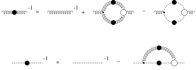
FIG. 1.: Diagrammatic representation of the truncated system of gluon and ghost DSEs.

Asymptotic expansions of the solutions in the infrared yield the leading infrared behaviour analytically. It is thereby uniquely determined by one exponent $\kappa=(61-\sqrt{1897})/19\approx 0.92$,

$$Z(k^{2})\,\stackrel{{\scriptstyle k^{2}\to 0}}{{\sim}}\,\left(\frac{k^{2}}{\sigma^{2}}\right)^{2\kappa}\quad\mbox{and}\quad G(k^{2})\,\stackrel{{\scriptstyle k^{2}\to 0}}{{\sim}}\,\left(\frac{\sigma^{2}}{k^{2}}\right)^{\kappa}\;,$$ (16)

for which the bounds $0<\kappa<1$ can be established requiring consistency with Slavnov–Taylor identities [10]. The renormalization group invariant momentum scale $\sigma$ represents a free parameter at this point which is later on fixed by choosing a definite value for the strong coupling constant at some scale. The qualitative infrared behavior in eqs. (16) has been also found by studies of further truncated DSEs [18]. Neither does it thus seem to depend on the particular 3-point vertices nor on employed approximations for angular integrals. All these solutions agree qualitatively and confirm the Kugo–Ojima confinement criterion.

There are also recent lattice simulations which test this criterion directly[19]. Instead of $u^{ab}=-\delta^{ab}$ they obtain numerical values of around $u=-0.7$ for the unrenormalized diagonal parts and zero (within statistical errors) for the off-diagonal parts. Taking into account the finite size effects on the lattices employed in the simulations, these preliminary results might still comply with the Kugo-Ojima confinement criterion.

Fig. 2: DSE solutions for $Z(x)$ and $G(x)$[10].

Fig. 3: $D(t,\hbox{\bf p}^{2})$ from DSEs for the gluon renormalization function $Z$ in Fig. 1.

Positivity violations of transverse gluon states are manifest in the spectral representation of the gluon propagator,

$$D(p^{2}):=\frac{Z(p^{2})}{p^{2}}=\int_{0}^{\infty}dm^{2}\,\frac{\rho(m^{2})}{p^{2}+m^{2}}\;.$$ (17)

From color antiscreening and unbroken global gauge symmetry in QCD it follows that the spectral density asymptotically is negative and superconvergent [3, 4, 5]

$$\rho(k^{2})\stackrel{{\scriptstyle k^{2}\to\infty}}{{\sim}}-\frac{\gamma g^{2}}{k^{2}}\Big{(}g^{2}\ln\frac{k^{2}}{\Lambda^{2}}\Big{)}^{-\gamma-1}\hskip-8.5359pt,\quad\mbox{and}\;\int_{0}^{\infty}\!\!dm^{2}\rho(m^{2})=\left(\frac{g_{0}^{2}}{g^{2}}\right)^{\gamma}\to 0\;,$$ (18)

since $\gamma>0$ for $N_{f}\leq 9$ in Landau gauge. This implies that it contains contributions from quartet states (and does therefore not need to be gauge invariant unlike in QED). Here, we consider the one-dimensional Fourier transform

$$D(t,\hbox{\bf p}^{2})=\int\frac{dp_{0}}{2\pi}\frac{Z(p_{0}^{2}+\hbox{\bf p}^{2})}{p_{0}^{2}+\hbox{\bf p}^{2}}\;e^{ip_{0}t}\,=\,\int_{\sqrt{\mbox{\bf p}^{2}}}^{\infty}d\omega\,\rho(\omega^{2}\!-\!\mbox{\bf p}^{2})\,e^{-\omega t}\;,$$ (19)

which for $\rho\geq 0$ had to be positive definite (and one had $\frac{d^{2}}{dt^{2}}\ln D(t,\hbox{\bf p})\geq 0$). This is clearly not the case for the DSE solution shown in Fig. 1 which violates reflection positivity [5, 10]. Even though no negative $D(t,\hbox{\bf p}^{2})$ have been reported in lattice calculations yet, the available results [20] agree in indicating that ln $D(t,\hbox{\bf p}^{2})$ is not the convex function of the Euclidean time it should be for positive $\rho$ [21, 22]. These are non-perturbative verifications of the positivity violation for transverse gluon states which already occur in perturbation theory. More significant for confinement is the fact that no massless single transverse gluon contribution to $\rho$ exists for $Z(0)=0$.

Fig. 4: The gluon renormalization function from the DSE solutions of Ref. [10] (solid line) and from the lattice data of Ref. [23].

Fig. 5: The ghost propagator from DSEs in Ref. [10] (solid line) compared to data and fit (dashed with $ca^{2}=0.744,\;da^{4}=0.256$ for $x\geq 2$) from Ref. [26].

Confirmation of the important result that the gluon renormalization function vanishes in the infrared and no massless asymptotic transverse gluon states occur, i.e., $Z(0)=0$, is seen in Fig. 1, where the DSE solution of Fig. 1 is compared to lattice data [23] and it was further verified recently with improved lattice actions for large volumes [13]. This infrared suppression as seen in lattice calculations thereby seems to be weaker than the DSE result, apparently giving rise to an infrared finite gluon propagator $D(k)\sim Z(k^{2})/k^{2}$ (corresponding to an exponent $\kappa=1/2$ in (16)), but a vanishing one does not seem to be ruled out for the infinite volume limit [24]. Similar results with finite $D(0)$ are also reported from the Laplacian gauge which practically avoids Gribov copies [25].

The infrared enhanced DSE solution for ghost propagator is compared to lattice data in Fig. 1. One observes quite compelling agreement, the numerical DSE solution fits the lattice data at low momenta ($x\leq 1$) significantly better than the fit to an infrared singular form with integer exponents, $D_{G}(k^{2})=c/k^{2}+d/k^{4}$. Though low momenta ($x<2$) were excluded in this fit, the authors concluded that no reasonable fit of such a form was otherwise possible [26]. Therefore, apart from the question about a possible maximum at the very lowest momenta, the lattice calculation seems to confirm the infrared enhanced ghost propagator with a non-integer exponent $0<\kappa<1$. The same qualitative conclusion has in fact been obtained in a more recent lattice calculation of the ghost propagator in $SU(2)$ [24], where its infrared dominant part was fitted best by $D_{G}\sim 1/(k^{2})^{1+\kappa}$ for an exponent $\kappa$ of roughly $0.3$ (for $\beta=2.7$).

To summarize, the qualitative infrared behavior in eqs. (16), an infrared suppression of the gluon propagator together with an infrared enhanced ghost propagator as predicted by the Kugo-Ojima criterion for the Landau gauge, is confirmed by the presently availabe lattice calculations. The exponents obtained therein ($0.3<\kappa\leq 0.5$) both seem to be consistently smaller than the one obtained in solving their DSEs. Whether also the lattice data is thereby determined by one unique exponent $0<\kappa<1$ for the infrared behavior of both propagators, has not yet been investigated to our knowledge. An independent confirmation of this combined infrared behavior which is indicative of an infrared fixed point would support the existence of the unphysical massless states that are necessary to circumvent the decomposition property for colored clusters.

Acknowledgements

R. A.  thanks Sebastian Schmidt and David Blaschke for organizing this stimulating workshop.

This work has been supported in part by the DFG under contract Al 279/3-3 and under contract We 1254/4-2.

SU(2) gluon propagators from the lattice –
a preview

Kurt Langfeld

Institut für Theoretische Physik, Universität Tübingen,
Auf der Morgenstelle 14, D–72076 Tübingen, Germany

PACS: 11.15.Ha 12.38.Aw

keywords: Landau gauge, Gribov problem, gluon propagator, confinement, lattice gauge theory.

Introduction. Two prominent methods to treat non-perturbative Yang-Mills theory will be addressed in this talk: the numerical simulation of lattice gauge theory (LGT) and the approach by means of the Dyson-Schwinger equations (DSE). While LGT covers all non-perturbative effects and, in particular, bears witness of quark confinement (see e.g. [1]), simulations including dynamical quarks are cumbersome despite the recent successes by improved algorithms [2] and the increase of computational power. At the present stage, systems at finite baryon densities are hardly accessible in the realistic case of an SU(3) gauge group [3] (for recent successes see [4]). By contrast, the DSE approach can be easily extended for an investigation of quark physics [5, 6] even at finite baryon densities [7]. Unfortunately, the DSE approach requires a truncation of the infinite tower of equations, and this approximation is difficult to improve systematically. In addition, the DSE approach needs gauge fixing which is obscured by Gribov copies. Whether the standard Faddeev-Popov method of gauge fixing is appropriate in non-perturbative studies, is still under debate [8].

In order to merge the advantages of both approaches to low energy Yang-Mills theory, I will firstly address the gluon propagator of pure SU(2) lattice gauge theory in Landau gauge. The result can then be compared with the one provided by the solution of the coupled ghost-gluon Dyson equation [9, 11, 12]. This will allow us to estimate the soundness of the truncations introduced to solve the equations (e.g. vertex ansatz, angular approximation). Secondly, the gluon propagator is an one essential ingredient of the quark DSE. Two options are obvious: a parameterization of the lattice result for the gluon propagator enters the quark DSE. The corresponding solution of this equation provides informations on hadronic observables in quenched approximation i.e. the backreaction of the quarks on the gluonic Greenfunctions is neglected. Once the reliability of the DSE approach to the ghost gluon system has been tested, the second option is to solve a truncated set of coupled ghost-gluon-quark DSEs, thereby, challenging the quenched approximation.

In my talk, I will focus on the gluon propagator as inferred from the lattice calculation, and I will concentrate on the information on quark confinement which might be encoded in the gluon propagator. High accuracy data for the latter are obtained by a numerical method superior to existing techniques. Further informations and details of the numerical method will be presented in a forthcoming publication.

Lattice definition of the gluon field. Before identifying the gluonic degrees of freedom in the lattice formulation, I briefly recall the definition of the gluon field in continuum Yang-Mills theory.

The starting point for constructing Yang-Mills theories is the transformation property of the matter fields. In the case of an SU(2) gauge theory, we demand invariance under local SU(2) (say color) transformations of the quark fields

$$q^{\prime}(x)\;=\;\Omega\,(x)\;q(x)\;,\hbox to28.45274pt{\hfill}\Omega(x)\in{\mathrm{S}U(2)}\;.$$ (1)

In order to construct a gauge invariant kinetic term for the quark fields, one defines the gauge covariant derivative $D_{\mu}:=\partial_{\mu}+iA_{\mu}^{a}t^{a}$, where $t^{a}$ are the generators of the SU(2) gauge group. Per definitionem, this covariant derivative homogeneously transforms under gauge transformations,

$$D^{\prime}_{\mu}q^{\prime}(x)\;=\;\Omega(x)\,D_{\mu}(x)\,q(x)$$ (2)

if the gluon fields transforms as

$$A^{a\,\prime}_{\mu}(x) = O^{ab}(x)\,A^{b}_{\mu}(x)\;+\;f^{aef}\,O^{ec}(x)\,\partial_{\mu}O^{fc}\;,$$ (3)

$$O^{ab}(x) := 2\,\mbox{Tr}\,\bigl{\{}\Omega(x)\,t^{a}\,\Omega^{\dagger}(x)\,t^{b}\bigr{\}}\;,\hbox to28.45274pt{\hfill}O^{ab}(x)\,\in\,{\mathrm{S}O(3)}\;.$$ (4)

The crucial observation is that the gluon fields transform according to the adjoint representation while the matter fields are defined in the fundamental representation.

Let us compare these definitions of fields with the ones in LGT. In LGT, a discretization of space-time with a lattice spacing $a$ is instrumental. The ’actors’ of the theory are SU(2) matrices $U_{\mu}(x)$ which are associated with the links of the lattice. These links transform under gauge transformations as

$$U^{\prime}_{\mu}(x)\;=\;\Omega(x)\,U_{\mu}(x)\,\Omega^{\dagger}(x+\mu)\;\hbox to28.45274pt{\hfill}\Omega(x)\in{\mathrm{S}U(2)}\;.$$ (5)

For comparison with the ab initio continuum formulation, I also introduce the adjoint links

$$\widetilde{U}_{\mu}^{ab}(x) := 2\,\mbox{Tr}\,\bigl{\{}U_{\mu}(x)\,t^{a}\,U^{\dagger}_{\mu}(x)\,t^{b}\bigr{\}}\;,$$ (6)

$$\widetilde{U}_{\mu}^{\prime}(x) := O(x)\,\widetilde{U}_{\mu}(x)\,O^{T}(x)\;,\hbox to28.45274pt{\hfill}O(x)\in{\mathrm{S}O(3)}\;,$$ (7)

where $O(x)$ was defined in (4).

In order to define the gluonic fields from lattice configurations, I exploit the behavior of the (continuum) gluon fields under gauge transformations (see (3)), and identify the lattice gluon fields $\hat{A}_{\mu}^{a}(x)$ as algebra fields of the adjoint representation, i.e.

$$\widetilde{U}_{\mu}^{ab}(x)\;=:\;\biggl{[}\exp\bigl{\{}\epsilon^{f}\,\hat{A}^{f}_{\mu}(x)\,a\bigr{\}}\,\biggr{]}^{ab}\;,\hbox to28.45274pt{\hfill}\big{(}\epsilon^{f}\bigr{)}^{ac}:=\epsilon^{afc}\;,$$ (8)

where the total anti-symmetric tensor $\epsilon^{abc}$ acts as generator for the SU(2) adjoint representation, and where $a$ denotes the lattice spacing.

For later use, it is convenient to have an explicit formula for the (lattice) gluon fields $\hat{A}_{\mu}^{a}(x)$ in terms of the SU(2) link variables $U_{\mu}(x)$. Usually, these links are given in terms of four vectors of unit length

$$U_{\mu}(x)\;=\;u_{\mu}^{0}(x)\,+\,i\,\vec{u}_{\mu}(x)\,\vec{\tau}\;,\hbox to28.45274pt{\hfill}\bigl{[}u^{0}_{\mu}(x)\bigr{]}^{2}\,+\,\bigl{[}\vec{u}_{\mu}(x)\bigr{]}^{2}\;=\;1\;,$$ (9)

where $\tau^{b}$ are the Pauli matrices. Using these variables, a straightforward calculation yields

$$\hat{A}^{b}_{\mu}(x)\,a\;+\;{\cal O}(a^{2})\;=\;2\,u^{0}_{\mu}(x)\,u^{b}_{\mu}(x)\;,\hbox to113.81102pt{ without summation over }\,\mu\;.$$ (10)

I point out that (14) is a novel definition of the lattice gluon field.

Finally, I illustrate the definition (14). Let us assume that we have exploited the gauge degrees of freedom (see (1)) to bring the SU(2) link elements $U_{\mu}(x)$ as close as possible to the unit matrix,

$$\Omega(x):\;\sum_{\{x\},\mu}\mbox{Tr}\,\,U^{\prime}_{\mu}(x)\rightarrow\,\mathrm{max}\;.$$ (11)

In this gauge, I decompose the link variables by

$$U^{\prime}_{\mu}(x)\;=\;Z_{\mu}(x)\,\exp\biggl{\{}i\hat{A}^{b}_{\mu}(x)\,t^{b}\,a\biggr{\}}\;,$$ (12)

where $\hat{A}^{b}_{\mu}(x)$ is implicitly defined by (11) and $Z_{\mu}(x)\in\{-1,+1\}$. Indeed, the lattice gluon fields (14) do not change when $U_{\mu}(x)\rightarrow(-1)U_{\mu}(x)$. Hence, the fields $\hat{A}^{b}_{\mu}(x)$ are relegated to the SO(3) coset space. I here propose to disentangle the information carried by the center and coset parts of the link variables by studying the $Z_{\mu}(x)$ and $\hat{A}^{b}_{\mu}(x)$ correlation functions independently. I stress, however, that in Landau gauge (15) the role of the $Z_{\mu}(x)$ is de-emphasized ($Z_{\mu}(x)\rightarrow 1$). In particular, I do not expect a vastly different gluon propagator when other (more standard) definitions of the lattice gluon fields are used [13, 14].

Gauge fixing. In the continuum formulation, calculations employing gauge fixed Yang-Mills theory use only gauged gluon fields which satisfies the gauge condition, e.g.

$$\partial_{\mu}A^{\prime\,a}_{\mu}(x)\;=0\;\hbox to85.35826pt{\hfill(Landau gauge) \hfill}\;,$$ (13)

and rely on the assumption that the Faddeev-Popov determinant corrects the probabilistic weight in an appropriate way. This assumption is true if the gauge condition picks a unique solution $\Omega(x)$ of (13) for a given field $A^{a}_{\mu}(x)$. Unfortunately, the Landau gauge condition generically admits several solutions depending on the ”background field” $A_{\mu}^{b}(x)$ which is the subject of gauge fixing (Gribov problem). Thus, the above assumption seems not always be justified [8]. Further restrictions on the space of possible solutions are required [15].

Let us contrast the continuum gauge fixing with its lattice analog. In a first step, link configurations $U_{\mu}(x)$ are generated by means of the gauge invariant action without any bias to a gauge condition. In a second step, the gauge-fixed ensemble is obtained by adjusting the gauge matrices $\Omega(x)$ (see (1)) until the gauged link ensemble satisfies the gauge condition. This procedure obviously guarantees the correct probabilistic measure for the gauged configurations, and gauge invariant quantities which are calculated with the gauged configurations evidently coincide with the ones obtained from un-fixed configurations. However, the Gribov problem re-appears as the problem of finding ”the name of the gauge”. Let me illustrate this last point: The naive Landau gauge condition for the lattice gluon field, i.e.

$$\hat{\partial}_{\mu}\hat{A}^{\prime\,b}_{\mu}(x)\;=\;0$$ (14)

is satisfied if we seek an extremum of the variational condition (15). If we restrict the variety of solutions $\Omega(x)$ which extremize (15) to those solutions which maximize the functional (15), we confine ourselves to the case where the Faddeev-Popov matrix is positive semi-definite. The fraction of the configuration space of gauge fixed fields $\hat{A}^{\prime\,b}_{\mu}$ is said to lie within the first Gribov horizon. A numerical algorithm which obtains the gauge transformation matrices $\Omega(x)$ from the condition (15) still samples a particular set of local maxima. Different algorithms might differ in the subset of chosen local maxima, and, hence, implement different gauges. A conceptual solution to the problem is to restrict the configuration space of gauge fixed fields $\hat{A}^{\prime\,b}_{\mu}$ to the so-called fundamental modular region. In the lattice simulation, this amounts to picking the global maximum of the variational condition (15). In practice, finding the global maximum is a highly non-trivial task. Here, I adopt two extreme cases of gauge fixing: firstly, I will study the gluon propagator of the gauge where an iteration over-relaxation algorithm almost randomly averages over the local maxima of the variational condition (15). This result will then be compared with the gluon propagator of a gauge where a simulated annealing algorithm searches for the global maximum. It will turn out that the gluon propagators of both gauges agree within statistical error bars.

The numerical simulation: The link configurations are generated using the Wilson action. I refrain from using a ”perfect action” since I am interested in the gluon propagator in the full momentum range; simulations using perfect actions recover a good deal of continuum physics at finite values of the lattice spacing at the cost of a non-local action. For practical simulations, perfect actions are truncated which is poor approximation at high energies where the full non-locality of the action must come into play.

Here, calculations were performed using a $16^{3}\times 32$ lattice. The dependence of the lattice spacing on $\beta$ (renormalization), i.e.

$$\sigma a^{2}(\beta)\;=\;0.12\,\exp\biggl{\{}-\frac{6\pi^{2}}{11}\,\bigl{(}\beta-2.3\bigr{)}\biggl{\}}\,,\hbox to28.45274pt{\hfill}\sigma:=(440\,{\mathrm{M}eV})^{2}\;,$$ (15)

is appropriate for $\beta\in[2.1,2.6]$ for the achieved numerical accuracy.

Once gauge-fixed ensembles are obtained by implementing a variational gauge condition (see discussion of previous section), the gluon propagator is calculated using

$$D^{ab}_{\mu\nu}(x-y)\;=\;\bigl{\langle}\hat{A}^{a}_{\mu}(x)\,\hat{A}^{b}_{\nu}(y)\,\bigr{\rangle}_{MC}\;,$$ (16)

where the Monte-Carlo average is taken over 200 properly thermalized gauge configurations. Of particular interest is the gluonic form factor $F(p^{2})$ which is defined by

$$D(p^{2})\;=\;\int D^{aa}_{\mu\mu}(x)\;\exp\bigl{\{}ipx\bigr{\}}\;d^{4}x\;,\hbox to28.45274pt{\hfill}D(p^{2})=\frac{F(p^{2})}{p^{2}}\;.$$ (17)

Since in Landau gauge the propagator is diagonal in color and transversal in Lorentz space, the form factor $F(p^{2})$ contains the full information.

TABLE I.: Simulation parameters: $L=32a$: lattice extension, $\Lambda$: UV cutoff

$\beta$	2.1	2.2	2.3	2.4	2.5
L [fm]	8.6	6.6	5.0	3.8	2.9
$\Lambda$ [GeV]	2.3	3.0	4.0	5.2	6.8

Results I: Landau gauge The lattice momentum in units of the lattice spacing is given by

$$p_{x}\,a\;=\;2\,\sin\left(\frac{\pi}{N}n_{x}\right)\;,\hbox to28.45274pt{\hfill}x=1\ldots 4$$ (18)

where $n_{x}$ is an integer which numbers the Matsubara frequency and $N$ is the number of lattice points (in $x$-direction).

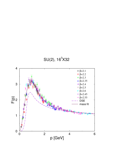
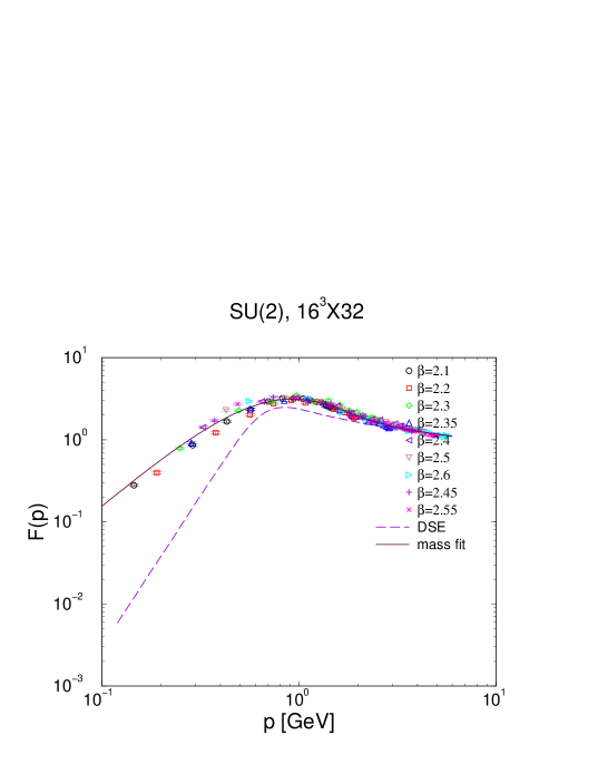
FIG. 1.: The gluonic form factor $F(p^{2})$ as function of the momentum transfer (left panel: linear scale; right panel: log-log scale). Also shown is the solution of the set of DSEs proposed in [9] which have been solved for the case of $SU(2)$ [10].

Physical units for the momentum can be obtained by using (15). Calculations with different $\beta$-values correspond to simulations with a different UV-cutoff $\Lambda:=\pi/a(\beta)$. In order to obtain the renormalized gluon propagator, the gluonic wave function renormalization is chosen to yield a finite (given) value for the form factor at fixed momentum transfer.

Figure 1 shows my result for the form factor $F(p^{2})$ where the condition (15) was implemented with an iteration over-relaxation method. The data obtained with different $\beta$-values are identical within numerical accuracy, thus signaling a proper extrapolation to the continuum limit.

At high momentum the lattice data are consistent with the behavior known from perturbation theory,

$$F(p^{2})\;\propto\;1/\left[log\frac{p^{2}}{\mu^{2}}\right]^{13/22}\;,\hbox to28.45274pt{\hfill}p^{2}\gg\mu^{2}\approx(1\,\mathrm{GeV})^{2}\;.$$ (19)

The lattice data are compared with the solution of the gluon-ghost DSE [9]. From the DSE studies one expects a scaling law at small momentum

$$F(p^{2})\;\propto\left[p^{2}\right]^{2\kappa}\;,\hbox to28.45274pt{\hfill}p^{2}\ll\mu^{2}\approx(1\,\mathrm{GeV})^{2}\;.$$ (20)

Depending on the truncation of the Dyson tower of equations and on the angular approximation of the momentum loop integral, one finds $\kappa=0.92$ [9] or $\kappa=0.77$ [11] or $\kappa\rightarrow 1$ [12]. The lattice data are consistent with $\kappa=0.5$ corresponding to an infrared screening by a gluonic mass. Also shown is the coarse grained ”mass fit” ($\mu=1\,$GeV)

$$F(p^{2})\;=\;\frac{p^{2}}{p^{2}+m_{1}^{2}}\biggl{[}\frac{\mu^{4}}{p^{4}+m_{2}^{4}}\;+\;\frac{s}{\left[log\left(\frac{m_{l}^{2}}{\mu^{2}}+\frac{p^{2}}{\mu^{2}}\right)\right]^{13/22}}\biggr{]}$$ (21)

which nicely reproduces the lattice data within the statistical error bars.

Results II: gluon propagator and confinement In order to get a handle on the information of quark confinement encoded in the gluon propagator in Landau gauge, I now change by hand the SU(2) Yang-Mills theory to a theory which does not confine quarks. It is instructive to compare the gluon propagator of the modified theory with the SU(2) result (see figure 1).

In the Maximal Center gauge [16], the mechanism of quark confinement can be understood by a percolation of vortices which acquire physical relevance in the continuum limit [17]. An intuitive picture in terms of vortex physics is also available for the deconfinement phase transition at finite temperatures [18]. Reducing the full Yang-Mills configurations to their vortex content still yields the full string tension [16]. Vice versa, removing these vortices from the Yang-Mills ensemble results in a vanishing string tension. This observation was used in [19] to verify the impact of the vortices on chiral symmetry breaking.

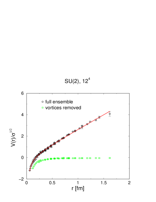
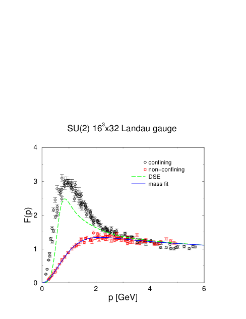
FIG. 2.: The static quark anti-quark potential (left panel) and the corresponding gluonic form factors (right panel); DSE solution from [10].

The static quark anti-quark potential in figure 2 demonstrates that a removal of the center vortices produces a non-confining theory. Figure 2 also shows the gluonic form factor obtained from the modified ensemble. The striking feature is that the strength of the form factor in the infra-red momentum range is drastically reduced.

Results III: the Gribov noise Finally, let us check how strongly the gluonic form factor $F(p^{2})$ depends on the choice of gauge, i.e. on the sample of maxima of the variational condition (15) selected by the algorithm. For this purpose, I adopt an extreme point of view by comparing the gauge implemented by the iteration over-relaxation (IA) algorithm with the gauge obtained by simulated annealing (SA). The results of the form factor in both cases are shown in figure 3. I find, in agreement with [13], that, in the case of the gluonic form factor, the Gribov noise is comparable with statistical noise for data generated with $\beta\in[2.1,2.5]$ (scaling window).

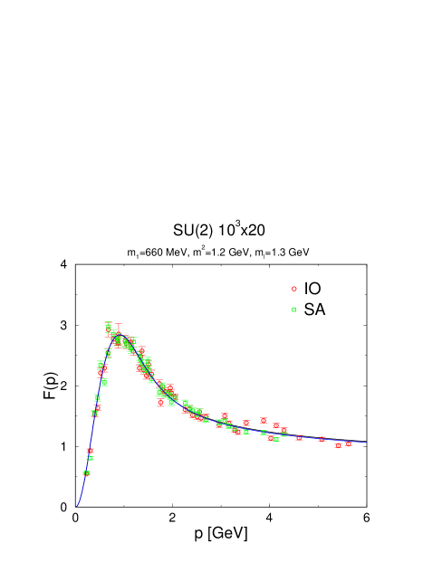
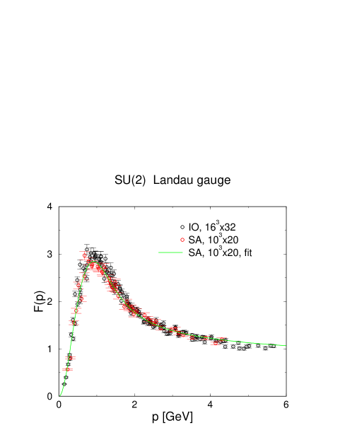
FIG. 3.: The gluonic form factor $F(p^{2})$ for a $10^{3}\times 20$ lattice in the gauge IA and SA, respectively (left panel) and compared with previous results (IA, $16^{3}\times 32$) (right panel).

Acknowledgements. I thank my coworkers J. Gattnar and H. Reinhardt. I am indebted to J. Bloch, R. Alkofer and Chr. Fischer for helpful discussions.

Gaugeless Unconstrained QCD and Monopoles

Victor Pervushin

BLTP, Joint Institute for Nuclear Research, 141980 Dubna, Russia

A Introduction

The consistent dynamic description of gauge constrained systems was one of the most fundamental problems of theoretical physics in the 20th century. There is an opinion that the highest level of solving the problem of quantum description of gauge relativistic constrained systems is the Faddeev-Popov (FP) integral for unitary perturbation theory [2]. In any case, just this FP integral was the basis to prove renormalizability of the unified theory of electroweak interactions in papers by ’t Hooft and Veltman marked by the 1999 Nobel prize.

Another opinion is that the FP integral has only the intuitive status. The most fundamental level of the description of gauge constrained systems is the derivation of ”equivalent unconstrained systems” (EUSs) compatible with the simplest variation methods of the Newton mechanics and with the simplest quantization by the Feynman path integral. It was the topic of Faddeev’s paper [1] ” Feynman integral for singular Lagrangians” where the non-Abelian EUS was obtained (by explicit resolving the Gauss law), in order to justify the intuitive FP path integral [2] by its equivalence to the Feynman path integral. Faddeev managed to prove the equivalence of the Feynman integral to the FP one only for the scattering amplitudes [1] where all particle-like excitations of the fields are on their mass-shell. However, this equivalence is not proved and becomes doubtful for the cases of bound states, zero modes and other collective phenomena where these fields are off their mass-shell. It is just the case of QCD. In this case, the FP integral in an arbitrary relativistic gauge can lose most interesting physical phenomena hidden in the explicit solutions of constraints [3, 4].

The present paper is devoted to the derivation an EUS for QCD in the class of functions of topologically nontrivial transformations, in order to present here a set of arguments in favor of that physical reasons of hadronization and confinement in QCD can be hidden in the explicit solutions of the non-Abelian constraints.

B Equivalent Unconstrained Systems in QED

The Gauss law constraint is the equation for the time component of a gauge field

$$\frac{\delta W}{\delta A_{0}}=0~{}\Rightarrow~{}~{}~{}\partial_{j}^{2}A_{0}=\partial_{k}\dot{A}_{k}+J_{0}$$ (1)

in the frame of reference with an axis of time $l^{(0)}_{\mu}=(1,0,0,0)$. Heisenberg and Pauli [5] noted that the gauge ($\partial_{k}A^{*}_{k}\equiv 0$) is distinguished, and Dirac [6] constructed the corresponding (”dressed”) variables $A^{*}$ in the explicit form

$$ieA^{*}_{k}=U(A)(ieA_{k}+\partial_{k})U(A)^{-1}~{},~{}~{}~{}~{}~{}~{}~{}~{}U(A)=\exp[ie\frac{1}{\partial_{j}^{2}}\partial_{k}A_{k}]~{},$$ (2)

using for the phase the time integral of the spatial part of the Gauss law $\partial_{k}\dot{A}_{k}$. The action for an EUS for QED is derived by the substitution of the solution of the Gauss law in terms of the ”dressed” variables into the initial action

$$W_{\rm Gauss-shell}=W^{*}_{l^{(0)}}(A^{*},E^{*})~{}.$$ (3)

The peculiarity of the EUS for QED is the electrostatic phenomena described by the monopole class of functions ($f(\vec{x})=O(1/r),|\vec{x}|=r\rightarrow\infty$).

The EUS can be quantized by the Feynman path integral in the form

$$Z_{F}[l^{(0)},J^{*}] = \int\limits d^{2}A^{*}d^{2}E^{*}$$ (5)

$$\exp\bigg{\{}iW^{*}_{l^{(0)}}[A^{*},E^{*}]+i\int\limits d^{4}x[J^{*}_{k}\cdot A^{*}_{k}-J_{0}^{*}\cdot A_{0}^{*}]\bigg{\}}$$

where $J^{*}$ are physical sources. This path integral depends on the axis of time $l^{(0)}_{\mu}=(1,0,0,0)$.

One supposes that the dependence on the frame ($l^{(0)}$) can be removed by the transition from the Feynman integral of the EUS  (5) to perturbation theory in any relativistic-invariant gauge $f(A)=0$ with the FP determinant

$$Z_{FP}[J]=\int\limits d^{4}A\delta[f(A)]\Delta_{FP}\exp\bigg{\{}iW[A]-i\int\limits d^{4}xJ_{\mu}\cdot A^{\mu}\bigg{\}}~{}.$$ (6)

This transition is well-known as a ”change of gauge”, and it is fulfilled in two steps
I) the change of the variables $A^{*}$ (2), and
II) the change of the physical sources $J^{*}$ of the type of

$$A^{*}_{k}(A)J_{k}^{*}=U(A)\left(A_{k}-\frac{i}{e}\partial_{k}\right)U^{-1}(A)J^{*}_{k}~{}\Rightarrow~{}A_{k}J^{k}~{}.$$ (7)

At the first step, all electrostatic monopole physical phenomena are concentrated in the Dirac gauge factor $U(A)$ (2) that accompanies the physical sources $J^{*}$.

At the second step, changing the sources (7) we lose the Dirac factor together with the whole class of electrostatic phenomena including the Coulomb-like instantaneous bound state formed by the electrostatic interaction.

Really, the FP perturbation theory in the relativistic gauge contains only photon propagators with the light-cone singularities forming the Wick-Cutkosky bound states with the spectrum differing from the observed one which corresponds to the instantaneous Coulomb interaction. Thus, the restoration of the explicit relativistic form of EUS($l^{(0)}$) by the transition to a relativistic gauge loses all electrostatic ”monopole physics” with the Coulomb bound states.

In fact, a moving relativistic atom in QED is described by the usual boost procedure for the wave function, which corresponds to a change of the time axis $l^{(0)}\Rightarrow l$, i.e., motion of the Coulomb potential [8] itself

$${W}_{C}=\int d^{4}xd^{4}y\frac{1}{2}J_{l}(x)V_{C}(z^{\perp})J_{l}(y)\delta(l\cdot z)\,\,\,,$$ (8)

where $J_{l}=l_{\mu}J^{\mu}\,\,,\,\,z_{\mu}^{\perp}=z_{\mu}-l_{\mu}(z\cdot l)\,\,,\,\,z_{\mu}=(x-y)_{\mu}\,\,.\,\,$ This transformation law and the relativistic covariance of EUS in QED has been predicted by von Neumann [5] and proven by Zumino [9] on the level of the algebra of generators of the Poincare group. Thus, on the level of EUS, the choice of a gauge is reduced to the choice of a time axis (i.e., the reference frame). A time axis is chosen to be parallel to the total momentum of a bound state, so that the coordinate of the potential always coincides with the space of the relative coordinates of the bound state wave function to satisfy the Yukawa-Markov principle [10] and the Eddington concept of simultaneity (”yesterday’s electron and today’s proton do not make an atom”) [11].

In other words, each instantaneous bound state in QED has a proper EUS, and the relativistic generalization of the potential model is not only the change of the form of the potential, but sooner the change of a direction of its motion in four-dimensional space to lie along the total momentum of the bound state. The relativistic covariant unitary perturbation theory in terms of instantaneous bound states has been constructed in [8].

C Unconstrained QCD

1 Topological degeneration and class of functions

We consider the non-Abelian $SU_{c}(3)$ theory with the action functional

$$W=\int d^{4}x\left\{\frac{1}{2}({G^{a}_{0i}}^{2}-{B_{i}^{a}}^{2})+\bar{\psi}[i\gamma^{\mu}(\partial_{\mu}+{\hat{A}_{\mu}})-m]\psi\right\}~{},$$ (9)

where $\psi$ and $\bar{\psi}$ are the fermionic quark fields. We use the conventional notation for the non-Abelian electric and magnetic fields

$$G_{0i}^{a}=\partial_{0}A^{a}_{i}-D_{i}^{ab}(A)A_{0}^{b}~{},~{}~{}~{}~{}~{}~{}B_{i}^{a}=\epsilon_{ijk}\left(\partial_{j}A_{k}^{a}+\frac{g}{2}f^{abc}A^{b}_{j}A_{k}^{c}\right)~{},$$ (10)

as well as the covariant derivative $D^{ab}_{i}(A):=\delta^{ab}\partial_{i}+gf^{acb}A_{i}^{c}$.

The action (9) is invariant with respect to gauge transformations $u(t,\vec{x})$

$${\hat{A}}_{i}^{u}:=u(t,\vec{x})\left({\hat{A}}_{i}+\partial_{i}\right)u^{-1}(t,\vec{x}),~{}~{}~{}~{}~{}~{}\psi^{u}:=u(t,\vec{x})\psi~{},$$ (11)

where ${\hat{A}_{\mu}}=g\frac{\lambda^{a}}{2i}A_{\mu}^{a}~{}$.

It is well-known [12] that the initial data of all fields are degenerated with respect to the stationary gauge transformations $u(t,\vec{x})=v(\vec{x})$. The group of these transformations represents the group of three-dimensional paths lying on the three-dimensional space of the $SU_{c}(3)$-manifold with the homotopy group $\pi_{(3)}(SU_{c}(3))=Z$. The whole group of stationary gauge transformations is split into topological classes marked by the integer number $n$ (the degree of the map) which counts how many times a three-dimensional path turns around the $SU(3)$-manifold when the coordinate $x_{i}$ runs over the space where it is defined. The stationary transformations $v^{n}(\vec{x})$ with $n=0$ are called the small ones; and those with $n\neq 0$

$${\hat{A}}_{i}^{(n)}:=v^{(n)}(\vec{x}){\hat{A}}_{i}(\vec{x}){v^{(n)}(\vec{x})}^{-1}+L^{n}_{i}~{},~{}~{}~{}~{}L^{n}_{i}=v^{(n)}(\vec{x})\partial_{i}{v^{(n)}(\vec{x})}^{-1}~{},$$ (12)

the large ones.

The degree of a map

$${\cal N}[n]=-\frac{1}{24\pi^{2}}\int d^{3}x~{}\epsilon^{ijk}~{}Tr[L^{n}_{i}L^{n}_{j}L^{n}_{k}]=n~{}.$$ (13)

as the condition for normalization means that the large transformations are given in the class of functions with the spatial asymptotics ${\cal O}(1/r)$. Such a function $L^{n}_{i}$ (12) is given by

$$v^{(n)}(\vec{x})=\exp(n\hat{\Phi}_{0}(\vec{x})),~{}~{}~{}~{}~{}\hat{\Phi}_{0}=-i\pi\frac{\lambda_{A}^{a}x^{a}}{r}f_{0}(r)~{},$$ (14)

where the antisymmetric SU(3) matrices are denoted by

$$\lambda_{A}^{1}:=\lambda^{2},~{}\lambda_{A}^{2}:=\lambda^{5},~{}\lambda_{A}^{3}:=\lambda^{7}~{},$$

and $r=|\vec{x}|$. The function $f_{0}(r)$ satisfies the boundary conditions

$$f_{0}(0)=0,~{}~{}~{}~{}~{}~{}~{}~{}~{}~{}~{}~{}~{}~{}f_{0}(\infty)=1~{},$$ (15)

so that the functions $L_{i}^{n}$ disappear at spatial infinity $\sim{\cal O}(1/r)$. The functions $L_{i}^{n}$ belong to monopole-type class of functions. It is evident that the transformed physical fields $A_{i}$ in (12) should be given in the same class of functions.

The statement of the problem is to construct an equivalent unconstrained system (EUS) for the non-Abelian fields in this monopole-type class of functions.

2 The Gauss Law Constraint

So, to construct EUS, one should solve the non-Abelian Gauss law constraint [3, 13]

$$\frac{\delta W}{\delta A_{0}}=0~{}~{}~{}~{}~{}\Rightarrow(D^{2}(A))^{ac}{A_{0}}^{c}=D_{i}^{ac}(A)\partial_{0}A_{i}^{c}+j_{0}^{a}~{},$$ (16)

where $j_{\mu}^{a}=g\bar{\psi}\frac{\lambda^{a}}{2}\gamma_{\mu}\psi$ is the quark current.

As dynamical gluon fields $A_{i}$ belong to a class of monopole-type functions, we restrict ouselves to ordinary perturbation theory around a static monopole $\Phi_{i}(\vec{x})$

$$A^{c}_{i}(t,\vec{x})={\Phi}^{c}_{i}(\vec{x})+\bar{A}^{c}_{i}(t,\vec{x})~{},$$ (17)

where $\bar{A}_{i}$ is a weak perturbative part with the asymptotics at the spatial infinity

$$\hat{\Phi}_{i}(\vec{x})=O(\frac{1}{r}),~{}~{}~{}~{}~{}~{}~{}~{}\bar{A}_{i}(t,\vec{x})|_{\rm asymptotics}=O(\frac{1}{r^{1+l}})~{}~{}~{}~{}(l>1)~{}.$$ (18)

We use, as an example, the Wu-Yang monopole [14, 15]

$$\Phi_{i}^{WY}=-i\frac{\lambda_{A}^{a}}{2}\epsilon_{iak}\frac{x^{k}}{r^{2}}f_{1}^{WY},~{}~{}~{}~{}~{}~{}~{}f^{WY}_{1}=1$$ (19)

which is a solution of classical equations everywhere besides the origin of coordinates. To remove a sigularity at the origin of coordinates and regularize its energy, the Wu-Yang monopole is changed by the Bogomol’nyi-Prasad-Sommerfield (BPS) monopole [16]

$$f^{WY}_{1}~{}\Rightarrow~{}f^{BPS}_{1}=\left[1-\frac{r}{\epsilon\sinh(r/\epsilon)}\right]~{},~{}~{}~{}~{}~{}\int\limits d^{3}x[B^{a}_{i}(\Phi_{k})]^{2}=\frac{4\pi}{g^{2}\epsilon}~{},$$ (20)

to take the limit of zero size $\epsilon~{}\rightarrow~{}0$ at the end of the calculation of spectra and matrix elements. This case gives us the possibility to obtain the phase of the topological transformations (14) in the form of the zero mode of the covariant Laplace operator in the monopole field

$$(D^{2})^{ab}({\Phi_{k}^{BPS}})({\Phi}_{0}^{BPS})^{b}(\vec{x})=0~{}.$$ (21)

The nontrivial solution of this equation is well-known [16]; it is given by equation (14) where

$$f_{0}^{BPS}=\left[\frac{1}{\tanh(r/\epsilon)}-\frac{\epsilon}{r}\right]$$ (22)

with the boundary conditions (15). This zero mode signals about a topological excitation of the gluon system as a whole in the form of the solution ${\cal Z}^{a}$ of the homogeneous equation

$$(D^{2}(A))^{ab}{\cal Z}^{b}=0~{},$$ (23)

i.e., a zero mode of the Gauss law constraint (16) [13, 17] with the asymptotics at the space infinity

$$\hat{\cal Z}(t,\vec{x})|_{\rm asymptotics}=\dot{N}(t)\hat{\Phi}_{0}(\vec{x})~{},$$ (24)

where $\dot{N}(t)$ is the global variable of this topological excitation of the gluon system as a whole. From the mathematical point of view, this means that the general solution of the inhomogeneous equation (16) for the time-like component $A_{0}$ is a sum of the homogeneous equation (23) and a particular solution ${\tilde{A}}_{0}^{a}$ of the inhomogeneous one (16): $A_{0}^{a}={\cal Z}^{a}+{\tilde{A}}^{a}_{0}$ .

The zero mode of the Gauss constraint and the topological variable $N(t)$ allow us to remove the topological degeneration of all fields by the non-Abelian generalization of the Dirac dressed variables (2)

$$0=U_{\cal Z}(\hat{\cal Z}+\partial_{0})U_{\cal Z}^{-1}~{},~{}~{}~{}~{}{\hat{A}}^{*}_{i}=U_{\cal Z}({\hat{A}}^{I}+\partial_{i})U_{\cal Z}^{-1},~{}~{}~{}\psi^{*}=U_{\cal Z}\psi^{I}~{},$$ (25)

where the spatial asymptotics of $U_{\cal Z}$ is

$$U_{\cal Z}=T\exp[\int\limits^{t}dt^{\prime}\hat{\cal Z}(t^{\prime},\vec{x})]|_{\rm asymptotics}=\exp[N(t)\hat{\Phi}_{0}(\vec{x})]=U_{as}^{(N)}~{},$$ (26)

and $A^{I}=\Phi+\bar{A},\psi^{I}$ are the degeneration free variables with the Coulomb-type gauge in the monopole field

$$D_{k}^{ac}(\Phi)\bar{A}^{c}_{k}=0~{}.$$ (27)

In this case, the topological degeneration of all color fields converts into the degeneration of only one global topological variable $N(t)$ with respect to a shift of this variable on integers: $(N~{}\Rightarrow~{}N+n,~{}n=\pm 1,\pm 2,...)$. One can check [18] that the Pontryagin index for the Dirac variables (25) with the assymptotics (18), (24), (26) is determined by only the diference of the final and initial values of the topological variable

$$\nu[A^{*}]=\frac{g^{2}}{16\pi^{2}}\int\limits_{t_{in}}^{t_{out}}dt\int\limits d^{3}xG^{a}_{\mu\nu}{}^{*}G^{a\mu\nu}=N(t_{out})-N(t_{in})$$ (28)

The considered case corresponds to the factorization of the phase factors of the topological degeneration, so that the physical consequences of the degeneration with respect to the topological nontrivial initial data are determined by the gauge of the sources of the Dirac dressed fields $A^{*},\psi^{*}$

$$W^{*}_{l^{(0)}}(A^{*})+\int\limits d^{4}xJ^{c*}A^{c*}=W^{*}_{l^{(0)}}(A^{I})+\int\limits d^{4}xJ^{c*}A^{c*}(A^{I})~{}.$$ (29)

The nonperturbative phase factors of the topological degeneration can lead to a complete destructive interference of color amplitudes [3, 17, 19] due to averaging over all parameters of the degenerations, in particular

$$<1|\psi^{*}|0>=<1|\psi^{I}|0>\lim\limits_{L\to\infty}\frac{1}{2L}\sum\limits_{n=-L}^{n=+L}U_{as}^{(n)}(x)=0~{}.$$ (30)

This mechanism of confinement due to the interference of phase factors (revealed by the explicit resolving the Gauss law constraint [3]) disappears after the change of ”physical” sources $A^{*}J^{*}~{}\Rightarrow~{}AJ$ (that is called the transition to another gauge). Another gauge of the sources loses the phenomenon of confinement, like a relativistic gauge of sources in QED (7) loses the phenomenon of electrostatics in QED.

3 Physical Consequences

The dynamics of physical variables including the topological one is determined by the constraint-shell action of an equivalent unconstrained system (EUS) as a sum of the zero mode part, and the monopole and perturbative ones

$$W^{*}_{l^{(0)}}=W_{Gauss-shell}=W_{\cal Z}[N]+W_{mon}[\Phi_{i}]+W_{loc}[\bar{A}]~{}.$$ (31)

The action for an equivalent unconstrained system (31) in the gauge (27) with a monopole and a zero mode has been obtained in the paper [18] following the paper [1]. This action contains the dynamics of the topological variable in the form of a free rotator

$$W_{\cal Z}=\int\limits dt\frac{{\dot{N}}^{2}I}{2};~{}~{}~{}I=\int\limits_{V}d^{3}x(D^{ac}_{i}(\Phi_{k})\Phi^{c}_{0})^{2}=\frac{4\pi}{g^{2}}(2\pi)^{2}\epsilon~{},$$ (32)

where $\epsilon$ is a size of the BPS monopole considered as a parameter of the infrared regularization which disappears in the infinite volume limit. The dependence of $\epsilon$ on volume can be chosen so that the density of energy was finite. In this case, the U(1) anomaly can lead to additional mass of the isoscalar meson due to its mixing with the topological variable [18]. The vacuum wave function of the topological free motion in terms of the Ponryagin index (28) takes the form of a plane wave $\exp(iP_{N}\nu[A^{*}])$. The well-known instanton wave function [20] appears for nonphysical values of the topological momentum $P_{N}=\pm i8\pi^{2}/g^{2}$ that points out the possible status of instantons as nonphysical solutions with the zero energy in Euclidean space-time . In any case, such the Euclidean solutions cannot describe the phenomena of the type of the complete destructive interference (30).

The Feynman path integral for the obtained unconstrained system in the class of functions of the topological transformations takes the form (see [18])

$$Z_{F}[l^{(0)},J^{a*}] = \int\limits DN(t)\int\limits\prod\limits_{c=1}^{c=8}[d^{2}A^{c*}d^{2}E^{c*}]$$ (34)

$$\times\exp\left\{iW^{*}_{l^{(0)}}[A^{*},E^{*}]+i\int\limits d^{4}x[J^{c*}_{\mu}\cdot A^{c*}_{\mu}]\right\}~{},$$

where $J^{c*}$ are physical sources.

The perturbation theory in the sector of local excitations is based on the Green function $1/D^{2}(\Phi)$ as the inverse differential operator of the Gauss law which is the non-Abelian generalization of the Coulomb potential. As it has been shown in [18], the non-Abelian Green function in the field of the Wu-Yang monopole is the sum of a Coulomb-type potential and a rising one. This means that the instantaneous quark-quark interaction leads to spontaneous chiral symmetry breaking [8, 21], goldstone mesonic bound states [8], glueballs [21, 22], and the Gribov modification of the asymptotic freedom formula [22]. If we choose a time-axis $l^{(0)}$ along the total momentum of bound states [8] (this choice is compatible with the experience of QED in the description of instantaneous bound states), we get the bilocal generalization of the chiral Lagrangian-type mesonic interactions [8].

The change of variables $A^{*}$ of the type of (2) with the non-Abelian Dirac factor

$$U(A)=U_{\cal Z}\exp\left\{\frac{1}{D^{2}(\Phi)}D_{j}(\Phi)\hat{A}_{j}\right\}$$ (35)

and the change of the Dirac dressed sources $J^{*}$ can remove all monopole physics, including confinement and hadronization, like similar changes (2), (7) in QED (to get a relativistic form of the Feynman path integral) remove all electrostatic phenomena in the relativistic gauges.

The transition to another gauge faces the problem of zero of the FP determinant $detD^{2}(\Phi)$ (i.e. the Gribov ambiguity [23] of the gauge (27)). It is the zero mode of the second class constraint. The considered example (34) shows that the Gribov ambiguity (being simultaneously the zero mode of the first class constraint) cannot be removed by the change of gauge as the zero mode is the inexorable consequence of internal dynamics, like the Coulomb field in QED. Both the zero mode, in QCD, and the Coulomb field, in QED, have nontrivial physical consequences discussed above, which can be lost by the standard gauge-fixing scheme.

D Instead of Conclusion

The variational methods of describing dynamic systems were created for the Newton mechanics. All their peculiarities (including time initial data, spatial boundary conditions $O(1/r)$, time evolution, spatial localization, the classification of constraints, and equations of motion in the Hamiltonian approach) reflect the choice of a definite frame of reference distinguished by the axis of time $l^{(0)}_{\mu}=(1,0,0,0)$. This frame determines also the EUS for the relativistic gauge theory. This equivalent system is compatible with the simplest variational methods of the Newton mechanics. The manifold of frames corresponds to the manifold of ”equivalent unconstrained systems”. The relativistic invariance means that a complete set of physical states for any equivalent system coincides with the one for another equivalent system [24].

This Schwinger’s treatment of the relativistic invariance is confused with the naive understanding of the relativistic invariance as independence on the time-axis of each physical state. The latter is not obliged, and it can be possible only for the QFT description of local elementary excitations on their mass-shell.

For a bound state, even in QED, the dependence on the time-axis exists. In this case, the time-axis is chosen to lie along the total momentum of the bound state in order to get the relativistic covariant dispersion law and invariant mass spectrum. This means that for the description of the processes with some bound states with different total momenta we are forced to use also some corresponding EUSs. Thus, a gauge constrained system can be completely covered by a set of EUSs. This is not the defect of the theory, but the method developed for the Newton mechanics.

What should we choose to prove confinement and compute the hadronic spectrum in QCD: equivalent unconstrained systems obtained by the honest and direct resolving of constraints, or relativistic gauges with the lattice calculations in the Euclidean space with the honest summing of all diagrams that lose from the very beginning all constraint effects?

Acknowledgments

I thank Profs. D. Blaschke, J. Polonyi, and G. Röpke for critical discussions. This research and the participation at the workshop “Quark matter in Astro- and Particle Physics” was supported in part by funds from the Deutsche Forschungsgemeinschaft and the Ministery for Education, Science and Culture in Mecklenburg- Western Pommerania.

Confinement as crossover

Janos Polonyi

polonyi@fresnel.u-strasbg.fr
Laboratory of Theoretical Physics, Louis Pasteur University
3 rue de l’Université 67084 Strasbourg, Cedex, France
Department of Atomic Physics, L. Eötvös University
Pázmány P. Sétány 1/A 1117 Budapest, Hungary

A Introduction

Having no systematic derivation of the confining forces in pure Yang-Mills theories the studies of the long range properties of the hadronic vacuum are usually based on model computations [1]-[4]. In order to get closer to the understanding of the problem it is obviously better to use models which contain at least partially the original gluonic degrees of freedom.

The bag model [1] is based on weakly interacting quarks and gluons, the confinement is realized by the difference of the energy density of two different vacua: inside and outside of the bag. No colored degrees of freedom are supposed to exist outside. The boundary of the bag, considered as a dynamical degree of freedom is obviously non-renormalizable. In the Abelian dual superconductor model [2] the Schwinger relation which asserts that the electric and the magnetic charges are inversely proportional to each other indicates that the magnetic condensate is due to a non-renormalizable coupling constant. The stochastic confining model [3] does not shed light on this question since it is based on the cluster expansion leaving the origin of the correlations an open question. The invariant Haar-measure terms of the functional integral which yield the string tension within the haaron model [4] are non-renormalizable, as well.

It is worthwhile noting that haaron model is the only one where the non-renormalizable term which is responsible for the string tension is already present in the original asymptotically free Yang-Mills Lagrangian. In fact, the gauge invariant, non-perturbative lattice regularization is based on the invariant Haar measure for the gauge group valued link variables. The logarithm of the Haar measure, treated as a local interaction potential in the action is non-polynomial and thereby non-renormalizable. Nevertheless the cut-off can be removed by suppressing these vertices sufficiently fast in the continuum limit [5].

We are confronted with an interesting possibility: How can it happen that the leading infrared force of the Yang-Mills theory comes from non-renormalizable vertices? The string tension, being a dimensionful parameter, can be generated by a relevant operator only. Since the non-renormalizable terms are irrelevant these vertices influence the interaction at the cut-off scale only and could have been left out from the theory according to the universality. The solution of this apparent paradox is rather simple [6]: Any theory with internal scale has at least two scaling regimes, an UV and an IR one, separated by a crossover at the internal scale. The non-renormalizable vertices are indeed irrelevant in the UV scaling regime but they might become relevant at the IR side of the crossover, in the IR scaling regime, where the IR forces are generated.

Section B overviews briefly the symmetry and the order parameter related to the confinement. An effective theory, the haaron model, to describe confinement as a destructive interference is mentioned in Section C. The lesson of the manner the confining force is generated in this model is discussed in Section D. The finite temperature aspects of confinement as a crossover phenomenon are touched upon in Section E. Finally, Section F is for the conclusion.

B Order parameter and destructive interfence

The order parameter for confinement is given in terms of the analytically continued massive quark propagator,

$$\Omega(x,t)=tr\langle\psi(x,t)\bar{\psi}(x,t+i\beta)\rangle,$$ (1)

where the trace is over the color and the spin indices and $\beta=1/T$. Note that for infinitely heavy quarks in a time independent environment this expression reduces to the Polyakov line

$$\omega(x)=trPe^{i\int_{0}^{\beta}d\tau A_{0}(x,\tau)}$$ (2)

up to a constant multiplicative factor, where $A_{0}(x,\tau)$ is the temporal component of the Euclidean gauge field.

$\Omega$ displays the status of the symmetry with respect to the center of the gauge group which is the group $Z_{n}$ for the gauge group $SU(n)$. The order parameter can be easily introduced even for Yang-Mills models in continuous Minkowski space-time [7] and it remains a manifestly gauge invariant, well defined observable.

The dynamical quarks make the picture more complicated and we should distinguish two competing confinement mechanisms, a hard and a soft one. Both are driven by the increase of the effective coupling strength as the color charges are separated. The hard confining mechanism of the Yang-Mills models is responsible for the flux tube formation and the linearly rising potential between a static quark-anti quark pair. The soft mechanism is due to the Dirac-sea polarization and, similarly to the supercritical vacuum of QED [8], shields the isolated quarks [9]. The soft mechanism cuts short the hard one and saturates the linearly rising potential when the flux tube between a static quark-anti quark pair is broken by the polarization of the Dirac-sea.

This ”deconfining ” vacuum-polarization effect appears in the dynamics of our order parameter, as well: The formal center symmetry is broken by the fermion determinant in the grand canonical ensemble. But it is easy to see that the Legendre transformation of the baryon number between the canonical and the grand canonical ensemble is ill defined in the thermodynamical limit due to the confinement mechanism. In fact, the free energy is infinitely large for states with non-vanishing triality which turns the free energy into a non-differentiable function of the baryon number density in the thermodynamical limit, and the control of the baryon number by a chemical potential into a highly non-trivial problem [10]. It is the canonical ensemble for the triality [10], [11] which should rather be used in this case and this ensemble is formally center symmetrical. But this formal symmetry is broken spontaneously at low temperatures [10]. At high temperature the center symmetry is broken dynamically by the gluon kinetic energy. There is no reason to expect that the two unrelated symmetry breaking mechanisms would generate the same expectation value for $\Omega$ thereby (1) remains to be an order parameter which experiences a non-analytic dependence on the environmental variables at the deconfinement transition [10].

The dynamical picture of confinement with $SU(n)$ as color gauge group is the following [7]: The configuration space for global gauge rotations, $SU(n)/Z_{n}$, is multiply connected. Its fundamental group, the center $Z_{n}$ can be used to lump the time-dependent gluon field configurations into $n$-tuples in such a manner that the trajectories of an $n$-tuple correspond to the same initial or end points in the multiply connected space $SU(n)/Z_{n}$ but differ on the covering space, $SU(n)$. The center symmetry of the pure gluonic system makes the action $S$ of the trajectories of an $n$-tuple degenerate in the absence of quarks. Thus the contribution of $n$ trajectories of an $n$-tuple to the transition amplitude is

$${\cal A}_{E}=ne^{-S},~{}~{}~{}{\cal A}_{M}=ne^{iS}$$ (3)

in Euclidean and Minkowski space-time. When a spectator quark is propagating along with the gluons then it picks up the $Z_{n}$ phase of the center transformation and the contribution of an $n$-tuple is vanishing due to the destructive interference between the homotopy classes,

$${\cal A}_{E}=\sum_{\ell=1}^{n}e^{i{2\pi\over n}\ell-S},~{}~{}~{}{\cal A}_{M}=\sum_{\ell=1}^{n}e^{i{2\pi\over n}\ell+iS}.$$ (4)

Notice that the non-positive definite phase factor comes from the projection operator which is supposed to install Gauss’ law and may lead to a destructive interference even for imaginary time. The semiclassical expansion, saturated by Wu-Yang monopoles in the Prasad-Sommerfeld limit [12] supports the confinement as a destructive interference phenomenon, as well.

For an $SU(2)$ gauge model the center symmetry expresses the invariance of a three vector under rotation by angle $2\pi$ and the destructive interference is due to the factor $-1$ the spinors of the fundamental representation collect during a rotation by $2\pi$.

The high temperature deconfining transition is due to the too high kinetic energy barrier for gluons to follow the trajectories in the whole homotopy class [7]. In the high temperature phase ”there is no time” to realize all homotopy class, the destructive interference is prohibited and quarks can propagate. Note that the kinetic energy driven dynamical symmetry breaking occurs at high energy or in short time processes contrary to the potential energy governed spontaneous symmetry breaking which is observed at low energy or long time. When dynamical quarks are present then the spontaneous breakdown of the center symmetry selects a homotopy class which dominates the sum (4) and leads to the screening of the isolated triality charge.

C Haaron model

We start this brief summary of the haaron model with a remark about the importance of keeping the exact gauge invariance in a computation to extract the string tension in Yang-Mills theory. Suppose that gauge invariance is implemented in an approximate manner and the state with a static quark-anti quark pair is $|q\bar{q}\rangle_{0}+|q\bar{q}\rangle_{1}$ where $|q\bar{q}\rangle_{0}$ has the proper transformation rule under gauge transformations and $|q\bar{q}\rangle_{1}$ not. The non-covariant component $|q\bar{q}\rangle_{1}$ appears to contain uncontrollable charge distribution. The expression

$$\left(\langle q\bar{q}|_{0}+\langle q\bar{q}|_{1}\right)H\left(|q\bar{q}\rangle_{0}+|q\bar{q}\rangle_{1}\right)=\langle q\bar{q}|_{0}H|q\bar{q}\rangle_{0}+\langle q\bar{q}|_{1}H|q\bar{q}\rangle_{1}$$ (5)

for the static potential shows that the charges in the component $|q\bar{q}\rangle_{1}$ will break the flux tube for a sufficiently large separation of the test charges and saturate the potential. The gauge non-covariant components shield off the string tension when they are present with any small amplitude.

There is another indication of the strong relation between gauge invariance and the confining forces. The effective theory for the Polyakov line obtained in the strong coupling expansion shows that the minimum of the effective potential is at a vanishing value of the order parameter at low temperature due to the presence of the invariant Haar-measure for the gauge field [13]. The replacement of the Haar-measure with a non-compact measure may keep the gauge invariance intact at any finite order of the loop expansion but certainly would break it at a non-perturbative level.

Guided by these remarks we wish to base our effective theory for the confining forces on the invariant Haar-measure in the path integral. Consider $SU(2)$ Yang-Mills theory for simplicity where the center transformation amounts to $\Omega\to-\Omega$. The lattice regularized path integral is given as

$$\int D_{H}[aA_{\mu}(x)]e^{-S_{YM}[aA_{\mu}(x)]},$$ (6)

where $a$ stands for the lattice spacing. The invariant integration measure for $A_{0}^{j}(x)=u(x)\omega^{j}(x)$, $j=1,2,3$, $(\omega^{j}(x))^{2}=1$ can be written as

$$D_{H}[aA_{0}(x)]=D[\omega(x)]D[u(x)]e^{\sum_{x}\log\sin^{2}au(x)}$$ (7)

in terms of the flat integration measure $D[u(x)]$ for $u(x)$. The center transformation, $u(x)\to u(x)+\pi/a$, performed at a given equal-time hypersurface is a symmetry of the periodic potential $a^{-4}\log\sin^{2}au$ appearing in (7). Let us integrate out the UV modes from the path integral and lower the cut-off. This step makes the dimensional transmutation explicit and induces an effective gauge theory model with dimensional parameters. First we choose a gauge in this theory where the temporal component $A_{0}(x)$ is diagonal, $\omega^{a}(x)=\delta^{a,3}$ and then we set the non-diagonal components of the gauge field to zero, leaving behind a compact $U(1)$ gauge model. The Feynman gauge is chosen for this model. As the final step, we set the spatial component of the Abelian gauge field to zero. What we find at the end is an effective theory for the diagonal, temporal component of the original gauge field, $u(x)$. The corresponding effective action will be approximated in the framework of the gradient expansion by the form

$$S_{eff}[u]=\int d^{4}x\left[{1\over 2}(\partial_{\mu}u(x))^{2}-V(u(x))\right].$$ (8)

The potential, the remnant of the invariant Haar-measure is periodic $V(u+2\pi/\ell)=V(u)$. The periodicity reflects the discrete center symmetry of the original theory and allows the Fourier representation $V(u)=\sum_{n}v_{m}\cos m\ell u$. The center symmetry requires that the symmetry $u\to u+2\pi/\ell$ is respected by the vacuum. The obvious consequence of this symmetry is the absence of any barrier in the effective potential between the periodic minima. This leads to the flattening of the effective potential for $u$ and the masslessness of the field $u(x)$.

It is well known that the sine-Gordon model is equivalent with a Coulomb gas. The simplest way to see this is to expand the generating functional in the coupling constant $v$,

$$Z[\rho] = \int D[u]e^{-{1\over 2}u\cdot G^{-1}\cdot u+iu\cdot\rho+{1\over 2}v_{m}\int dx(e^{im\ell u(x)}+e^{-im\ell u(x)})}$$ (9)

$$= \sum_{n}{(v_{m}/2)^{n}\over n!}\prod_{j=1}^{n}\int dx_{j}\sum_{\sigma_{j}=\pm 1}\int D[u]e^{-{1\over 2}u\cdot G^{-1}\cdot u+iu\cdot(\rho+\sigma)}$$ (10)

$$= e^{-{1\over 2}\rho\cdot G\cdot\rho}\sum_{n}{(v_{m}/2)^{n}\over n!}\prod_{j=1}^{n}\int dx_{j}\sum_{\sigma_{j}=\pm 1}e^{-{1\over 2}\sigma\cdot G\cdot\sigma}e^{-\rho\cdot G\sigma},$$ (11)

where $G$ is the massless propagator and $\sigma(x)=m\ell\sum_{j=1}^{n}\sigma_{j}\delta(x-x_{j})$. This is the grand canonical partition function of a four dimensional gas of particles interacting with the inverse of the massless propagator, the Coulomb potential. The first exponential in the last line represents the perturbative self-interaction of the external source $\rho$, the second stands for the self-interaction of the particles and finally the third one describes the interaction between the source and the particles. Let us ignore the inter-particle forces and the partition function for non-interacting particles can be resummed,

$$Z[\rho]\approx e^{{1\over 2}\rho\cdot G\cdot\rho+{1\over 2}v_{m}\int dx\cos(im\ell\int dyG(x-y)\rho(y))}.$$ (12)

These steps, repeated for each Fourier modes give

$$Z[\rho] = \int D[u]e^{-\int d^{4}x[{1\over 2}(\partial_{\mu}u(x))^{2}-V(u(x))-i\rho(x)u(x)]}$$ (13)

$$\approx e^{-{1\over 2}\rho\cdot G\cdot\rho+\int dxV(i\int dyG(x-y)\rho(y))}.$$ (14)

The particles representing the vertices of the perturbation expansion are called haarons since their contributions come from the invariant measure of the original path integral.

It is worth mentioning three applications of the partial resummation (13). The leading long range part of the static potential between a quark-anti quark pair separated by $x$ is

$$-\int d^{3}yV\left({i\over|y|}-{i\over|y-x|}\right)\approx-2V^{\prime\prime}(0)|x|,$$ (15)

giving the string tension

$$\sigma=-2V^{\prime\prime}(0).$$ (16)

Notice that in the center symmetry broken phase there is no protection against mass generation and the massive propagator does not give linearly rising potential. Thus the measure term which gives vanishing contribution in the UV regime and is included to assure the full gauge invariance only actually generates the leading long range force. Since it generates a new dimensional parameter, the string tension, the measure term must be relevant in the IR regime.

The second application of the resummation gives a confining version of the NJL model. We start with the Lagrangian

$$L={1\over 2}(\partial_{\mu}u)^{2}-V(u)+i\bar{\psi}\partial_{\mu}\gamma^{\mu}\psi-igj~{},$$ (17)

where $j=u\bar{\psi}\gamma^{0}\sigma_{z}\psi$ and perform the free haaron gas resummation yielding

$$L_{eff} = i\bar{\psi}(x)\partial_{\mu}\gamma^{\mu}\psi(x)-V\left(ig\int d^{4}yG(x-y)j(y)\right)$$ (18)

$$\approx i\bar{\psi}(x)\partial_{\mu}\gamma^{\mu}\psi(x)-{1\over 2}g^{2}V^{\prime\prime}(0)\int d^{4}yj(x)G_{2}(x-y)j(y)$$ (19)

$$= i\bar{\psi}(x)\partial_{\mu}\gamma^{\mu}\psi(x)+g\sqrt{-V^{\prime\prime}(0)}j(x)\phi(x)+{1\over 2}\phi(x)\Box^{2}\phi(x)~{},$$ (20)

where

$$G_{2}(x-y)=\int d^{4}zG(x-z)G(z-y)=\int{d^{4}p\over(2\pi)^{4}}{1\over p^{4}}e^{-ip(x-y)}~{},$$ (21)

and the auxiliary field $\phi(x)$ was introduced in order to render the Lagrangian local. Notice that the $1/p^{4}$ propagator of the auxiliary field, coupled to the quarks in the same manner as $u(x)$, confines the color charges with a linearly rising potential and the string tension is (16).

The third application of the resummation is the computation of the quenched quark propagator. The grand canonical partition function, the last line of Eq. (9) when $\rho$ is replaced by the quark current $j(x)$ shows that the quarks are propagating in the imaginary long range field

$$u_{y,n}(x)={in\ell\over 4\pi^{2}(x-y)^{2}}$$ (22)

of the haarons. After performing the Wick rotation into Minkowski space-time this external field becomes real. The destructive interference between the homotopy classes appears in this effective model as the destructive interference between the scattering processes of a quark off the gas of haarons. The long range haaron field makes the phase shift diverging and the fast rotating phase of the scattered state cancels the quark propagator when the averaging over the haaron distributions is performed. In order to understand the propagation of a meson qualitatively let us assume that the haaron field at $x$ and $y$ is identical or completely uncorrelated when $|x-y|<\xi$ or $|x-y|>\xi$, respectively where $\xi\approx\Lambda^{-1}_{QCD}$ is the correlation length of the haaron gas. As long as the quark and the anti-quark of the meson propagates within the distance $\xi$ the phase shift suffered by them is canceled and the haarons do not influence much the propagation. When the color charges are separate from each other more than $\xi$ then the statistically independent phase shift suppresses the amplitude. The result is that the world lines can not separate more then the distance $\xi$, the confinement radius.

D Crossover in the vacuum

Let us consider the thought-experiment when the hadronic matter is viewed by a microscope of adjustable space-resolution. When details below the distance scale $\Lambda^{-1}_{QCD}$ are considered we find partons, i.e. quarks and gluons. As the resolution becomes worse and details on the scale well above $\Lambda^{-1}_{QCD}$ are seen only then hadrons and glueballs are found. The interactions between quarks and gluons on the one hand, and between hadrons on the other hand, are very different. This difference can simply be recorded by following the scale dependence generated by them.

There are at least two different scaling regimes in any non-scale invariant theory, an UV and an IR one separated by a crossover at the internal scale of the theory, $\Lambda^{-1}_{QCD}$ in our case, c.f. Fig. 1. The UV scaling reflects asymptotically free forces between quarks and gluons in the UV regime and short ranged Yukawa interactions among the asymptotic states, hadrons, on the IR side. In pure Yang-Mills theory glueballs are the asymptotic states in the IR and color charges remain strongly bound by the linearly rising potential. What was surprising in the haaron model picture is that the measure vertices of the action which are non-renormalizable, i.e. irrelevant in UV scaling regime can generate the leading long range force. There must be a change in the behavior of the measure vertices as we move towards the IR directions which explains their increased importance in the confining forces. The most natural scenario is that these operators, being irrelevant in the UV scaling regime become relevant in the IR side of the crossover.

This scenario raises a more general question, the possibility that non-renormalizable operators might play an important role in low energy physics. It is easy to see that this surprising phenomenon does not take place in models with mass gap $m\not=0$. These models display a correlation length $\xi\approx 1/m$ and the evolution of the running coupling constant slows down at distance $x\gg\xi$. In fact, the evolution of the coupling constants is driven by the contribution of the modes around the running cut-off and the fluctuations at the scale $x\gg\xi$ are suppressed by $\exp(-x/\xi)$. The absence of runaway trajectories of the renormalization group flow indicates that all non-Gaussian operators are irrelevant in the IR scaling regime.

Theories without mass gap may develop new relevant operators by the help of collinear or simple IR divergences which may drive the run-away trajectories. The $\phi^{4}$ model in the mixed phase possesses a non-renormalizable operator which is relevant at low energies [12]. The condensation mechanism in general can easily generate radically new scaling laws [15]. When gauge symmetry is protecting against mass generation then the four fermion interaction, the effective vertex responsible for the emergence of the BCS phase, turns out to be relevant at low energies [16]. The interaction vertices between hadronic states are irrelevant in QCD because the colorless sector is massive. The lesson of the haaron model is that the integral measure vertices become relevant in the IR scaling regime of the colored channels.

There are two ways to deal with changing scaling laws. The phenomenological approach is the matching where one introduces different models for the UV and the IR scaling regimes and tries to match them at the crossover. A more instructive procedure can be constructed by recalling one of the rules of the renormalization group studies: All coupling constants which are generated by the blocking and might turn out to be important should be present in the action from the very beginning. In fact, the renormalization group flow is a reliable source of information about the interactions only if the truncation of the space of Hamiltonians does not remove important pieces. This principle, applied to QCD suggests the introduction of colorless composite operators which control the hadronic states,

$$Z= \int D[\bar{\psi}]D[\psi]D_{H}[A_{\mu}]D[\bar{\chi}]D[\chi]D[\bar{\Psi}]D[\Psi]\times$$ (24)

$$e^{iS_{QCD}[\bar{\psi},\psi,A_{\mu}]+iS_{H}[\bar{\chi},\chi,\bar{\Psi},\Psi]+i\int dx(G_{\chi}\bar{\chi}\psi\psi\psi+G_{\Psi}\bar{\Psi}\bar{\psi}\psi+h.c.)},$$

the fields $\chi$ and $\Psi$ correspond to baryon and meson states and $S_{H}[\bar{\chi},\chi,\bar{\Psi},\Psi]$ is the action for a hadronic field theory. Since we are interested in the low energy phenomena we can fix the original cut-off at a sufficiently high but finite energy scale $\Lambda_{0}$. The coupling constants $G_{\chi}$ and $G_{\Psi}$ govern the strength of interactions between the hadronic and the colored states and their initial value is $G_{\chi}(\Lambda_{0})=G_{\Psi}(\Lambda_{0})=0$, together with the hadronic coupling constants in $S_{H}$. This scheme is not a double counting since it is cast in the path integral formalism, it is a possible parameterization of the effective action.

Such a hybrid model should hold the key to the understanding of the confinement phenomenon because it offers a singularity-free description of the crossover. As the cutoff is lowered the non-renormalizable coupling strengths remain small and the asymptotically free coupling $g$ grows. When the crossover is reached then $g$ explodes in perturbative QCD and an IR Landau-pole arises because the long range correlations of the ground state are supposed to be generated by the asymptotically free vertices. But such a hybrid model offers the following alternative. In the presence of operators which are important in the IR scaling regime there is a chance that $g$ stays finite because the desired long range correlations can be established first in the colored and after that in the neutral sector by the renormalization of the measure term as in the haaron model and the hadronic coupling constants, respectively.

E Crossover at high temperature

The real RHIC experiment is different, we are interested in the long distance correlations and quasiparticle structure at high temperature assuming that thermal equilibrium is an acceptable approximation. How does the temperature modify the scaling laws and the renormalized trajectory? It is obvious that the renormalized trajectory is in good approximation temperature independent at the observational length scale $x\ll 1/T$ and the temperature induced effects show up around $x\approx 1/T$, as shown qualitatively in Fig. 1. For $T<T_{dec}$ the clusterization of the color charges can be best understood as the impossibility of screening the $1/3$ color charge of a quark by multi-gluon states whose color charge is sum of integers, $\sum\pm 1\not=1/3$. The absence of screening mechanism leads to confining forces. The deconfining phase transition can be characterized in the Hamiltonian description by the improper implementation of the Gauss’ law projection operator which does not exclude certain states with infinitely many gluons. These states carry the color charge of a quark or anti-quark [7]. The result is the possibility of screening a quark color charge by a gluon cloud whose wave functional is multi-valued, the rearrangement of the infinite sum $\sum\pm 1$ in such an order that it converges to $1/3$. The effect of the temperature at the deconfining transition is the removal of the linear potential between triality charges by vacuum-polarization, a mechanism similar to the polarization of the Dirac-sea when dynamical quarks are present. A sort of soft confinement mechanism is operating in the high temperature phase of the pure glue system. The deconfined quarks are rendered colorless and only their flavor quantum numbers reveal their quark content.

The renormalization group flow of the pure glue system should have two different manifolds of IR fixed points, for $T>T_{dec}$ and $T<T_{dec}$, as shown in Fig. 1. The high temperature fixed points should be qualitatively similar to those of full QCD at low temperature, the role of quarks are being played by gluon states with multi-valued wave functionals.

FIG. 1.: The renormalization group flow of QCD shown for different temperatures. The solid line starting at the UV and ending at the IR fixed point, encircled by the limit of asymptotic scaling regimes, corresponds to $T=0$. The crossover separating the UV and IR scaling regimes is at $Cr$, $x\approx\Lambda^{-1}_{QCD}$. The flow at finite temperature displays temperature dependence when $x>1/T$ and gives two qualitatively different IR fixed point manifolds for $T<T_{dec}$ and $T>T_{dec}$.

For full QCD the difference between the low and the high temperature fixed point manifolds is more subtle since the soft confinement mechanism is operating in both phases, by means of quark or gluon states with multi-valued wave functionals. I believe that the quasiparticles of the high temperature fixed point are similar to those of the low temperature phase except that a new quark ”flavor” appears in the form of gluonic states with multi-valued wave functionals. The difference between the real and this fake quark can be detected by electro-weak currents only, the color charges being equivalent. The main features of this scenario are the screening of the color charge of the deconfined quark and the presence of the usual hadronic bound states. As of the former, a careful numerical study should be carried out measuring the gluonic color charge polarization around a deconfined quark. There are two indirect numerical evidences supporting the latter conjecture, the presence of the usual hadronic bound states. The first is the observation that the spacelike string tension is to a large extent temperature independent and remains non-vanishing even at high temperature [17], indicating that the equal time long-range correlations of the multi-quark states do not change at the deconfinement phase transition. Another result, indicating the unimportance of the string tension from the point of view of the structure of the hadronic states at $T=0$ is that the hadronic structure functions are qualitatively reproduced after cooling, a modification of the gluonic configurations which removes the string tension.

F Conclusion

It was argued in the framework of the haaron model that the leading long range forces between a quark-anti quark pair are generated by non-renormalizable vertices. This phenomenon motivates a look into the confinement problem following the strategy of the renormalization group and suggests that the confinement characterizes the IR scaling regime.

A lesson learned in dealing with the renormalization group is that all important operators should be present in the initial Hamiltonian even with vanishing coupling strength in order to understand the appearance of the dynamically generated, new kind of forces. Such a point of view motivates a hybrid model which contains both the quark-gluon and the hadronic fields. Their difference is set by the initial condition for the renormalization group flow only: a finite value for the asymptotically free coupling constant and a vanishing strength for the hadrons. The non-renormalizable measure term is supposed to generate a crossover in this model where the hadronic coupling constants turn on and induce the interactions of nuclear physics.

Such a description of the long range structure, together with the screening mechanism of the quark color charges by gluons available at high temperature suggests that the main difference between the high and the low temperature phases is not in the hadronic but rather in the quark sector of QCD. Possible examples are the following: The chromomagnetic monopoles, being ”hedgehog” configurations relate color and spin. The gluon polarization cloud around a deconfined quark with even or odd number of monopoles possesses integer or half-integer spin, respectively. In this manner the violation of the superselection rule for the charge induces a similar violation for the spin and the deconfined quark state is actually the sum of components with Bose and Fermi statistics [7]. Another triality-related effect is the deviation of the temperature of the quark and gluonic degrees of freedom at the deconfinement phase transition point, $T_{q}=T_{gl}/3$ [18].

Lattice simulations of QCD-like theories at non-zero density

Jonivar Skullerud

DESY Theory Group, Notkestraße 85, D–22603 Hamburg, Germany
Current address: ITF, Universiteit van Amsterdam, Valckenierstraat 65, 1018 XE Amsterdam, The Netherlands

A Introduction

Recently, there has been a considerable interest in QCD at non-zero chemical potential, after a number of model studies have indicated a rich phase structure [1, 2, 3] (for a review, see [4]). Clearly, it would be desirable if these predictions could be tested by first-principles, non-perturbative studies, e.g. lattice QCD. Unfortunately, lattice simulations of QCD at non-zero baryon density using standard methods are in practice impossible because the action (and the fermion determinant) becomes complex once the chemical potential is introduced, causing importance sampling to fail. It is possible to split the determinant into a modulus and a phase, simulating with the modulus of the determinant as the measure and reweighting the observables with the phase,

$$\langle O\rangle=\frac{\langle\langle O\,\mbox{arg(det}M)\rangle\rangle}{\langle\langle\mbox{arg(det}M)\rangle\rangle},$$ (1)

where $\langle\langle\ldots\rangle\rangle$ denotes the expectation value with respect to the positive real measure. However, the denominator in (1) is effectively the ratio of the partition functions of two different theories: the true theory and one with a positive real measure. This should scale as $\exp(-\Delta F)$, where $\Delta F$ is the difference in free energy between the two theories. Since the free energy is an extensive quantity, the computational effort required to obtain a reliable sample rises exponentially with the volume.

A number of approaches have been tried to overcome this problem (see [5] for a recent review). In the Hamiltonian formalism, the problem does not arise. Analytical results have been obtained in the strong coupling limit [6, 7], but so far no method for numerical simulations exists.

With an imaginary chemical potential [8], the action becomes real and positive, so simulations are straightforward. The problem is whether an analytical continuation to real $\mu$ is possible. It works at high temperature [9, 10], where also other approaches may be successfully employed [10], but does not seem to be possible at zero or low temperatures. Imaginary chemical potential can also be used to formulate a quenched limit of QCD in the background of a non-zero number of static quarks [11].

Cluster algorithms [12] may provide a way of eliminating the sign problem by summing analytically over configurations in a cluster in such a way that the contribution to the partition function from each cluster is always positive definite. So far, these methods have been applied to a number of spin models; however, an application to QCD has yet to be found.

Finally, the sign problem may be avoided by simulating theories which resemble QCD, but have a real action even at non-zero chemical potential. One such theory is QCD at non-zero isospin density [13, 14], which is of intrinsic interest because it corresponds to part of the phase diagram for asymmetric nuclear matter. Another class of theories encompasses two-colour QCD with fermions in the fundamental representation, as well as QCD with adjoint fermions, for any number of colours. The remainder of this review will focus on what can be learnt from lattice simulations of these theories.

B Theories with real action

The chemical potential $\mu$ is introduced on the lattice by multiplying the forward timelike links by $e^{\mu}$ and the backward timelike links by $e^{-\mu}$ [15]. It can be shown [16, 17] that the determinant $\det{M}$ of the fermion matrix $M$ in two-colour QCD is real, even for non-zero $\mu$, both in the continuum and on the lattice. However, it is only possible to demonstrate that it is positive [17] in the cases of continuum or Wilson adjoint fermions and staggered fundamental fermions. Indeed, we will see in section D that in the case of staggered adjoint fermions there are configurations with a negative determinant, leading to a sign problem at large $\mu$.

1 Symmetry breaking pattern

In the chiral limit, the action for two-colour QCD with $N$ flavours has a $\mathrm{U}(N)_{L}\otimes\mathrm{U}(N)_{R}$ symmetry, which for staggered fermions is manifest as independent $\mathrm{U}(N)$ symmetries for the even and odd sites. At $\mu=0$ this enlarges to a $\mathrm{U}(2N)$ symmetry. This can be seen most easily by introducing new fields,

$$\bar{X}_{e}=(\bar{\chi}_{e},-\chi^{T}_{e}\tau_{2})\qquad X_{o}=\left(\begin{array}[]{c}\chi_{o}\\ -\tau_{2}\bar{\chi}_{o}^{T}\end{array}\right)\\$$ (2)

for (staggered) fundamental quarks, and

$$\bar{X}_{e}=(\bar{\chi}_{e},\chi^{T}_{e})\qquad X_{o}=\left(\begin{array}[]{c}\chi_{o}\\ \bar{\chi}_{o}^{T}\end{array}\right)$$ (3)

for adjoint quarks. The action can then be written as

$$S={1\over 2}\sum_{x_{e},\nu}\eta_{\nu}(x)\biggl{[}\bar{X}_{e}(x) \left(\matrix{e^{\mu\delta_{\nu,0}}&0\cr 0&e^{-\mu\delta_{\nu,0}}\cr}\right) U_{\nu}(x)X_{o}(x+\hat{\nu})\,-$$ (4)

$$\bar{X}_{e}(x) \left(\matrix{e^{-\mu\delta_{\nu,0}}&0\cr 0&e^{\mu\delta_{\nu,0}}\cr}\right) U_{\nu}^{\dagger}(x-\hat{\nu})X_{o}(x-\hat{\nu})\biggr{]}$$ (5)

where $x_{e}$ denotes the even sites. In the continuum, the equivalent fields are

$$\text{fundamental:}\quad\Psi=\left(\begin{array}[]{c}\psi_{L}\\ \sigma_{2}\tau_{2}\psi_{R}^{*}\end{array}\right)\qquad\text{adjoint:}\quad\Psi=\left(\begin{array}[]{c}\psi_{L}\\ \sigma_{2}\psi_{R}^{*}\end{array}\right)$$ (6)

which gives the continuum lagrangian

$${\mathcal{L}}=i\Psi^{\dagger}\sigma_{\nu}(D_{\nu}-\mu B_{\nu})\Psi\,\qquad B_{\nu}=\left(\begin{array}[]{cc}1&0\\ 0&-1\end{array}\right)\delta_{\nu 0}\,.$$ (7)

The explicity chiral symmetry breaking term in the Wilson fermion action means that there is no equivalent enlarged symmetry for Wilson fermions; however, new fields may be introduced analogously to the continuum case, and the enlarged symmetries will be broken by ${\cal O}(a)$ terms in the action.

The chiral condensate can be written in terms of the new fields,

$$\bar{\chi}\chi=\bar{X}_{e}\!\left(\begin{array}[]{cc}0&1\kern-4.5pt1\\ \pm 1\kern-4.5pt1&0\end{array}\right)\!{T\over 2}\bar{X}_{e}^{tr}+X_{o}^{tr}\!\left(\begin{array}[]{cc}0&1\kern-4.5pt1\\ \pm 1\kern-4.5pt1&0\end{array}\right)\!{T\over 2}X_{o}$$ (8)

for staggered fermions, and

$$\bar{\psi}\psi=\Psi^{T}\sigma_{2}\frac{T}{2}\left(\begin{array}[]{cc}0&-1\kern-4.5pt1\\ \pm 1\kern-4.5pt1&0\end{array}\right)\Psi+{\rm h.c.}$$ (9)

in the continuum and for Wilson fermions. In both cases, the $+$ sign is for fundamental fermions and the $-$ sign for adjoint, while $T$ is $\tau_{2}$ for fundamental fermions and 1 for adjoint. A nonzero chiral condensate thereby breaks down the $\mathrm{U}(2N)$ symmetry to O($2N$) for fundamental fermions and Sp($2N$) for adjoint fermions, giving rise to $N(2N+1)$ and $N(2N-1)$ Goldstone modes respectively. Of these, there will be $N^{2}$ mesonic states, while the remaining $N(N\pm 1)$ will be diquarks. In the continuum, and for Wilson fermions, the pattern will be the opposite (modulo the 1 mode destroyed by the axial anomaly in the continuum), but for 1 flavour of fundamental quarks, there is no chiral symmetry in the first place. From this we see that in the case of $N=1$ adjoint staggered fermions, and only in this case, are there no diquark Goldstone modes.

For $m\neq 0$, all the pseudo-Goldstone modes remain degenerate, with masses $m_{\pi}\propto\sqrt{m}$. As the chemical potential $\mu$ increases, the ground state will begin to be populated with baryonic matter. The transition to a ground state containing matter occurs when $\mu=\mu_{o}\simeq m_{b}/n_{q}$, where $m_{b}$ is the mass of the lightest baryon, and this baryon contains $n_{q}$ quarks. At this point, the baryon number density $n$ becomes non-zero, where $n$ is given by

$$n =\frac{1}{2}\big{\langle} \bar{\psi}(x)e^{\mu}(\gamma_{0}-1)U_{0}(x)\psi(x+\hat{0})$$ (11)

$$+\bar{\psi}(x+\hat{0})e^{-\mu}(\gamma_{0}+1)U_{0}^{\dagger}(x)\psi(x)\big{\rangle}$$

for Wilson fermions, and

$$n=\frac{1}{2}\big{\langle}\bar{\chi}(x)\eta_{0}(x)[e^{\mu}U_{0}(x)\chi(x+\hat{0})+e^{-\mu}U_{0}^{\dagger}(x-\hat{0})\chi(x-\hat{0})]\big{\rangle}.$$ (12)

for staggered fermions. Where there are diquark Goldstone modes, those states will be the lightest baryons in the spectrum. This means that for most variants of two-colour QCD we expect $\mu_{o}\simeq m_{\pi}/2$, in contrast to the much larger value $m_{N}/3$ expected in real (three-colour) QCD. The exception is two-colour QCD with one flavour of adjoint staggered quarks.

In the limit of small $m$ and $\mu$, the behaviour of $\langle\bar{\psi}\psi\rangle$, the diquark condensate $\langle\psi\psi\rangle$, and $n$ as functions of $m$ and $\mu$ can be calculated in chiral perturbation theory. If we define the rescaled variables

$$x=\frac{2\mu}{m_{\pi 0}}\,,\quad y=\frac{\langle\bar{\psi}\psi\rangle}{\langle\bar{\psi}\psi\rangle_{0}}\,,\quad z=\frac{\langle\psi\psi\rangle}{\langle\bar{\psi}\psi\rangle_{0}}\,,\quad\tilde{n}=\frac{m_{\pi 0}n}{8m\langle\bar{\psi}\psi\rangle_{0}}\,,$$ (13)

where the 0 subscript denotes values at $\mu=0$, the prediction from $\chi$PT for the models with diquark Goldstone modes is [16]

$$y=\left\{\begin{array}[]{c}1\\ 1\over x^{2}\end{array}\right.\quad z=\left\{\begin{array}[]{c}0\\ \sqrt{1-\frac{1}{x^{4}}}\end{array}\right.\quad\tilde{n}=\left\{\begin{array}[]{cl}0&;x\!<\!1\\ {x\over 4}\left(1-{1\over x^{4}}\right)&;x\!>\!1\end{array}\right.$$ (14)

2 Diquark condensation

At large chemical potential, the relevant degrees of freedom will be quarks with momenta near the Fermi surface. The attractive quark–quark interaction will give rise to instability with respect to condensation of diquark pairs at opposite sides of the Fermi surface. In physical QCD, the diquark condensate cannot be a colour singlet, so the gauge symmetry is spontaneously broken, giving rise to the phenomenon of colour superconductivity.

In two-colour QCD, on the other hand, there may be the possibility of gauge singlet diquarks, which will be energetically favoured compared to non-singlet states. Indeed, in the previous section we saw that most variants of two-colour QCD have diquark Goldstone modes, which will be the preferred channel for diquark condensation. In the $N=1$ staggered adjoint model, this is not the case, and we do not know a priori in which channel the condensation will occur. We must proceed by constructing possible operators which obey the Pauli principle and making additional assumptions about locality, Lorentz structure and gauge invariance [17]. At least one of the possible condensates constructed this way gives rise to a colour superconding ground state.

The standard way of computing the diquark condensate on the lattice is to introduce a diquark source term into the action [18]. For two-colour QCD with fundamental staggered quarks the action then becomes

$$S_{F} = \sum_{x,y}\bar{\chi}(x)M_{xy}\chi(y)+\sum_{x}\frac{j}{2}\left[\chi^{T}(x)\tau_{2}\chi(x)+\bar{\chi}(x)\tau_{2}\bar{\chi}^{T}(x)\right]$$ (15)

$$= (\bar{\chi},\chi^{T})\left(\begin{array}[]{cc}j\tau_{2}&\frac{1}{2}M\\ \frac{1}{2}M&j\tau_{2}\end{array}\right)\left(\begin{array}[]{c}\!\bar{\chi}^{T}\\ \!\!\chi\end{array}\right)\equiv X^{T}{\mathcal{A}}[j]X\,.$$ (20)

In this case, the partition function becomes proportional to the Pfaffian $\text{Pf}{\mathcal{A}}[j]$. The diquark condensate $\langle\chi^{T}\tau_{2}\chi\rangle$ may be evaluated by taking

$$\langle\chi^{T}\tau_{2}\chi\rangle=\lim_{j\to 0}\frac{1}{2V}\left\langle\mathrm{Tr}\left\{{\mathcal{A}}^{-1}\left(\begin{array}[]{cc}\tau_{2}&0\\ 0&\tau_{2}\end{array}\right)\right\}\right\rangle$$ (21)

An alternative approach [19] is to rewrite the Pfaffian as

$$\mathrm{Pf}{\mathcal{A}}[j]=\mathrm{Pf}(B+j)=\pm\sqrt{\det(B+j)}$$ (22)

where

$$B=\left(\begin{array}[]{cc}0&\frac{1}{2}M\tau_{2}\\ -\frac{1}{2}M\tau_{2}&0\end{array}\right)\,.$$ (23)

This can be expanded as a polynomial in $j$ by diagonalising $B^{2}$, obviating the need to simulate at non-zero diquark source. Since this gives the Pfaffian at any $j$, it can also be used to determine the diquark condensate using the probability distribution function [20].

C Simulations with fundamental quarks

In the past year and a half, a number of groups have been performing lattice simulations of two-colour QCD with fundamental staggered fermions both at zero [21, 22, 23, 24, 14] and non-zero [25, 26] temperature. Also, one group is performing simulations with Wilson fermions [27].

Aloisio et al. [22, 23] have performed simulations in the strong coupling limit for a number of quark masses, flavours and lattice volumes. Fig. 1 shows results for the chiral condensate, the diquark condensate and the baryon number density, at $m=0.2$ and a non-zero source $j=0.02$, for two different lattice sizes. Also shown are the $\chi$PT predictions from (14). The agreement between the prediction and the numerical results is quite striking, considering that this is far from the continuum limit. This suggests a weak $\beta$ dependence. Fig. 2 shows the diquark condensate at zero diquark source, for $N_{f}=1$ and a range of quark masses. Again, we see a very good agreement with the prediction (14). At larger $\mu$, we see that the value of $\langle\psi\psi\rangle$ drops, going to zero at high $\mu$. This second transition is due to lattice artefacts connected with the saturation of lattice sites with fermions. In the infinite volume limit it is expected to disappear.

Simulations at non-zero $\mu$ with a diquark source have been performed by Kogut and Sinclair [14]. Results for the diquark condensate and chiral condensate are shown in fig. 3. Again, we see the chiral condensate dropping and the diquark condensate rising for $\mu\gtrsim m_{\pi}/2$, in agreement with $\chi$PT. We also see the same large-$\mu$ saturation behaviour for the diquark condensate as in [23]. Fig. 4 shows results for pion and scalar diquark masses. The scalar diquark mass falls roughly as $m_{\pi}-2\mu$ as $\mu$ approaches $m_{\pi}/2$. The pion mass remains constant up to $\mu\approx m_{\pi}/2$, after which it falls to zero. This is again in accordance with the expectation from $\chi$PT.

The spectrum of the Dirac operator has been studied in some detail by the Vienna group [24] for staggered fermions and by the Hiroshima group [27] for Wilson fermions. A preliminary study of topology at non-zero temperature has also been performed [25].

D Simulations with adjoint quarks

As indicated in section B 1, two-colour QCD with one flavour of adjoint staggered fermions has features which makes it in some senses more ‘QCD-like’ than other variants of two-colour QCD. In particular, it has no diquark Goldstone modes, so we expect an onset transition at a value of the chemical potential different from $m_{\pi}/2$ — possibly at $\mu=m_{N}/3$ where $m_{N}$ denotes the mass of the lightest three-quark baryon (the ‘nucleon’). It also has a sign problem.

The theory has been simulated [17, 28] using two different algorithms: Hybrid Monte Carlo, which is not able to change the sign of the determinant, and therefore only simulates the positive determinant sector of the theory, and the two-step multibosonic algorithm [29], which is able to take the sign properly into account. Figs 5 and 6 show the results from HMC simulations for $y$ and $\tilde{n}$ of (13) respectively, for a range of values for the quark mass $m$ and chemical potential $\mu$. Up to $x\sim 1.5$, the data collapse onto a universal curve, which agrees well with the predictions of (14). Even at larger $x$, the data for the chiral condensate lie close to the $\chi$PT prediction. At $x\gtrsim 2$, however, the data for different $m$ diverge, indicating that $\chi$PT may be breaking down. Results for the plaquette [28] show a drop in its value for $\mu\geq m_{\pi}/2$, presumably due to Pauli blocking, while the pion mass appears to agree with the $\chi$PT prediction $m_{\pi}=2\mu$ at $x>2$.

The agreement between the predictions of $\chi$PT and these results paradoxically enough presents a problem, since this model is not supposed to contain any diquark Goldstone modes, and thus the $\chi$PT predictions of (14) are not valid in this case. In particular, there should not be any onset transition at $\mu=m_{\pi}/2$. The suspicion must be that this contradiction is due to the fact that HMC does not change the sign of the determinant, and that it therefore simulates the wrong theory — a theory with conjugate quarks.

The simulation points for the TSMB algorithm were selected to focus on the effect of the sign, with one point at $\mu=0$, one just past the HMC onset transition, and one deeper into the dense region. With this algorithm, a reweighting factor $r$ and the sign of $\det{M}$ must be determined for each configuration [30]. The expectation value of an observable $O$ is then determined by the ratio

$$\langle O\rangle={{\langle O\times r\times sign\rangle}\over{\langle r\times sign\rangle}}.$$ (24)

The results for $\langle\bar{\psi}\psi\rangle$ and $n$, together with the corresponding HMC results, are summarised in Table I. For TSMB at $\mu\not=0$ we also include observables determined separately in each sign sector, defined by $\langle O\rangle_{\pm}=\langle O\times r\rangle_{\pm}/\langle r\rangle_{\pm}$. At $\mu=0.0$ the two algorithms agree, as they should. Also, the results in the positive determinant sector for TSMB at larger $\mu$ agree with the HMC results. However, the results for the negative determinant sector are significantly different. This difference has the effect of bringing the average both for $\langle\bar{\psi}\psi\rangle$ and for $n$ back to values consistent with the $\mu=0$ values. This is an indication that at $\mu=0.36$ and quite possibly also at $\mu=0.4$, the system is still in the vacuum phase, which means that the onset transition in this model occurs at a larger $\mu$ than for other variants of two-colour QCD. This is consistent with the symmetry-based arguments of section B 1 that this model has no baryonic Goldstone modes.

E Conclusions

Substantial progress has been made recently in lattice simulations of two-colour QCD at non-zero density, with both fundamental and adjoint quarks. The simulations with fundamental quarks nicely reproduce the predictions from chiral perturbation theory for the chiral condensate, diquark condensate, and baryon density, except at very large chemical potentials. Here, saturation effects are observed, especially for the diquark condensate. The meson and diquark spectrum is also being analysed, with preliminary results for the pion and scalar diquark masses again in rough agreement with chiral perturbation theory.

Two-colour QCD with one flavour of adjoint staggered quark is not expected to have any diquark Goldstone modes, unlike all other variants of two-colour QCD. It also has a sign problem. Simulations of this model restricted to the sector with a positive fermion determinant reproduce the predictions of chiral perturbation theory for theories with diquark Goldstone modes, including an early onset transition at $\mu\approx m_{\pi}/2$ — although the breakdown of $\chi$PT may be observed at larger $\mu$. When configurations with negative determinants are included, we find a strong correlation between the sign and the value of observables. This effect appears to lead to a cancellation of the early onset transition. This observation may hold the key to understanding the problem of the premature onset which has bedevilled previous attempts to simulate physical QCD at non-zero density.

The presence of diquark modes which are degenerate with the pion means that the study two-colour QCD is of limited usefulness when it comes to studying directly the onset transition, hadron spectrum and diquark condensation in physical QCD at non-zero density. However, useful experience may be gained by comparing the results of lattice simulations with those of other methods which are also applicable to physical QCD. Of particular interest would be the study of gluodynamics, where SU(2) and SU(3) are expected to exhibit similar behaviour, even at non-zero $\mu$. Thus it might be possible to cast light on the deconfinement transition at high $\mu$ and low $T$ by studying two-colour QCD.

Acknowledgments

This work is supported by the TMR network “Finite temperature phase transitions in particle physics”, EU contract ERBFMRX–CT97–0122.

FIG. 1.: Baryon density, chiral condensate and diquark condensate vs. chemical potential, from [22]. The solid lines are the predictions of (14).

FIG. 2.: Diquark condensate for a $6^{4}$ lattice, $N_{f}=1$, for $m=0.025$ (diamonds), 0.05 (squares) and 0.2 (stars) at strong coupling, from [23], with the predictions of (14).

FIG. 3.: Chiral condensate (left) and diquark condensate (right) vs. chemical potential, for one flavour fundamental staggered quarks, on an $8^{4}$ lattice; from [14]. The arrow indicates $\mu\approx m_{\pi}/2$.

FIG. 4.: Pion and scalar diquark masses as functions of chemical potential, for one flavour of fundamental staggered quarks, on an $8^{4}$ lattice; from [14]. The straight line is $m=m_{\pi}-2\mu$.

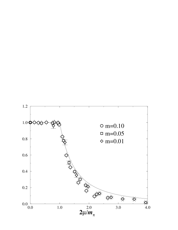
FIG. 5.: Chiral condensate vs. chemical potential for one flavour of adjoint staggered quarks, using the rescaled variables of eq. (13); from [28].

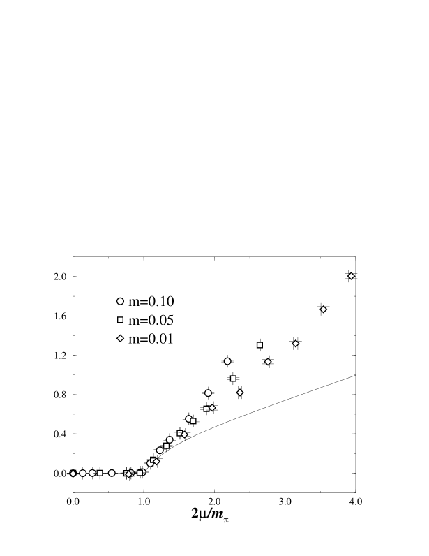
FIG. 6.: Baryon density vs. chemical potential for one flavour of adjoint staggered quarks, using the rescaled variables of eq. (13); from [28].

	$\mu$	TSMB			HMC
		$\langle O\rangle$	$\langle O\rangle_{+}$	$\langle O\rangle_{-}$
$\langle\bar{\chi}\chi\rangle$	0.0	1.526(2)			1.526(1)
	0.36	1.528(8)	1.507(7)	1.108(55)	1.497(5)
	0.4	1.59(13)	1.275(13)	1.177(14)	1.261(12)
$n$	0.0	$-0.0004(8)$			$-0.0002(3)$
	0.36	$-0.0053(66)$	0.0086(57)	0.279(35)	0.0203(41)
	0.4	$-0.041(84)$	0.138(11)	0.193(12)	0.1462(100)

TABLE I.: A comparison of results between TSMB and HMC for one flavour of adjoint staggered quarks. Due to long autocorrelation times, the errors in the HMC results may be underestimated.

Contributions on

Kinetic Theory and Heavy Ion Collisions

Kinetic Equations of QED Plasmas in Strong External Fields

A. Höll^†, V. Morozov^∗, G. Röpke^†

^†Rostock University, 18051 Rostock, Germany
^∗Moscow State Institute of Radioengineering, Electronics and Automation, Moscow, Russia

A Introduction

In recent years the theoretical study of high-temperature, dense relativistic plasmas occurring in astrophysics as well as in high-intense short-pulse lasers [1, 2] is of increasing interest. The nonequilibrium state of such systems consisting of fermions and photons should be described by relativistic covariant equations [3, 4, 5].

A particular point is the occurrence of strong fields which needs a special treatment when introducing perturbation theory. We will give a systematic approach within a Schrödinger picture. As an example, the kinetic equations in mean-field approximation are considered.

We use the system of units with $c=\hbar=1$. The signature of the metric tensor is $(+,-,-,-)$.

B Covariant Density Matrix Approach on Hyperplanes

A quantum system can be characterized by the knowledge of the state vector of the system $|\Psi\rangle$. It is determined by a complete set of commuting observables. In order to formulate a relativistic invariant theory we are lead to the question how measurements of observers in different frames of reference with respect to the system must be related with each other. Here we follow the idea of Bogoliubov, Fleming and others [6, 7, 8]. We define the operators and the state vector on spacelike hyperplanes $\sigma_{n,\tau}$ in Minkowski space. These planes are defined as

$$x\cdot n=\tau,\qquad n^{2}=n^{\mu}n_{\mu}=1,$$ (1)

with $n_{\mu}$ the unit normal vector of the plane and $\tau$ a scalar parameter. A special frame is the “laboratory” frame, were $n_{\mu}=(1,0,0,0)$ is a system with the observers being at rest with respect to the system.

Thus we write the state vector as a functional of the hyperplane $|\Psi[\sigma_{n,\tau}]\rangle$ and consider the operators $\hat{O}(n,\tau)$ as frame-dependent quantities. In what follows we will consider a Schrödinger picture formulation. That means that the operators are fixed to the initial plane chosen, whereas the state vector will evolve in timelike direction, i.e. depends on $\tau$. The space-time four-vector can always be decomposed as

$$x^{\mu}=n^{\mu}\tau+x^{\mu}_{\mbox{$\bot$}},\qquad\tau=n\cdot x,$$ (2)

where

$$x^{\mu}_{\mbox{$\bot$}}=\Delta^{\mu}_{\ \nu}\,x^{\nu},\quad\Delta^{\mu}_{\ \nu}=\delta^{\mu}_{\ \nu}-n^{\mu}n_{\nu}.$$ (3)

Now we must answer the question how state vectors located on different planes (i.e. state vectors measured by observers in different frames of references with respect to the system) are related with each other. In order to obtain a relativistic invariant formulation these state vectors must be related by Lorentz transformations (boosts) $\sigma^{\prime}=\Lambda\sigma$

$$\sigma\to\sigma^{\prime}=L\sigma:\quad x\to x^{\prime}=\Lambda x.$$ (4)

With $U(\Lambda)$ a unitary representation of the Lorentz transformation $\Lambda$ we can write

$$U(L)\left|\Psi[L\sigma]\right\rangle=\left|\Psi[\sigma]\right\rangle.$$ (5)

If we consider an infinitesimal timelike translation (i.e. in the direction of $n_{\mu}$) we can derive a relativistic Schrödinger equation

$$i\frac{\partial}{\partial\tau}\left|\Psi(n,\tau)\right\rangle=\hat{H}(n)\left|\Psi(n,\tau)\right\rangle$$ (6)

with the Hamiltonian on the hyperplane given by

$$\hat{H}(n)=\hat{P}_{\mu}n^{\mu}.$$ (7)

$P_{\mu}$ in Eq. (7) is the energy-momentum four vector.

Going now to a mixed quantum ensemble we can find the dynamical equation for the frame dependent statistical operator $\varrho(n,\tau)$

$$\frac{\partial\varrho(n,\tau)}{\partial\tau}-i\left[\varrho(n,\tau),\hat{H}^{\tau}(n)\right]=0.$$ (8)

In the “laboratory” frame Eq. (8) reduces to the von Neumann equation.

In order to proceed and to derive kinetic equtions for Schrödinger picture correlation functions, we needto define the quantum Hamiltonian, defined on the plane. A detailed discussion is presented in [9], which lead to

$$\hat{H}^{\tau}(n)=\hat{H}_{D}(n)+\hat{H}_{EM}(n)+\hat{H}_{\rm int}(n)+\hat{H}^{\tau}_{\rm ext}(n),$$ (9)

where $\hat{H}_{D}(n)$ and $\hat{H}_{EM}(n)$ are the Hamiltonians for free fermions and the electro-magnetic (EM) field (due to polarization) respectively, $\hat{H}_{\rm int}(n)$ is the interaction term, and $\hat{H}^{\tau}_{\rm ext}(n)$ describes the external EM field effects. In the Schrödinger picture the explicit expressions for these terms are

$$\hat{H}_{D}(n)=\int_{\sigma_{n}}d\sigma\,\,\hat{\!\bar{\psi}}\left(-\frac{i}{2}\gamma^{\mu}_{\mbox{$\bot$}}(n)\stackrel{{\scriptstyle\leftrightarrow}}{{\nabla}}_{\mu}+\,m\right)\hat{\psi}$$ (10)

$$\hat{H}_{EM}(n)=\int_{\sigma_{n}}d\sigma\,\left(\frac{1}{4}\hat{F}_{\mbox{$\bot$}\mu\nu}\hat{F}_{\mbox{$\bot$}}^{\mu\nu}-\frac{1}{2}\hat{\Pi}_{\mbox{$\bot$}\mu}\hat{\Pi}_{\mbox{$\bot$}}^{\mu}\right)$$ (11)

$$\hat{H}_{\rm int}(n)=\int_{\sigma_{n}}d\sigma\,\,\hat{\!j}_{\!\mbox{$\bot$}\mu}\hat{A}_{\mbox{$\bot$}}^{\mu}+\frac{1}{2}\int_{\sigma_{n}}d\sigma\int_{\sigma_{n}}d\sigma^{\prime}\,\,\hat{\!j}_{\!\mbox{$\|$}}(x_{\mbox{$\bot$}})G(x_{\mbox{$\bot$}}-x_{\mbox{$\bot$}}^{\prime})\,\hat{\!j}_{\!\mbox{$\|$}}(x_{\mbox{$\bot$}}^{\prime})$$ (12)

$$\hat{H}^{\tau}_{\rm ext}(n)=\int_{\sigma_{n}}d\sigma\,\,\hat{\!j}_{\!\mu}(x_{\mbox{$\bot$}}){A}^{\mu}_{\rm ext}(\tau,x_{\mbox{$\bot$}}).$$ (13)

In these equations we apply the Coulomb gauge condition on the plane $\nabla_{\mu}A^{\mu}_{\mbox{$\bot$}}=0$. Further $\hat{\Pi}_{\mbox{$\bot$}}^{\mu}$ is the canonical momentum to $\hat{A}^{\mu}_{\mbox{$\bot$}}$ and $G$ the Green function of the Poisson equation

$$\nabla_{\mu}\nabla^{\mu}G(x_{\mbox{$\bot$}})=\delta^{3}(x_{\mbox{$\bot$}}).$$ (14)

In the EM field Hamiltonian (11) the transverse field strength tensor was defined

$$\hat{F}^{\mu\nu}_{\mbox{$\bot$}}=\nabla^{\mu}\hat{A}^{\nu}_{\mbox{$\bot$}}-\nabla^{\nu}\hat{A}^{\mu}_{\mbox{$\bot$}},\qquad\nabla^{\nu}=\Delta_{\mu}^{\nu}\partial^{\mu}.$$ (15)

We can now observe the averaged values of the dynamical operators $\hat{A}^{\nu}_{\mbox{$\bot$}}$ and $\hat{\Pi}^{\nu}_{\mbox{$\bot$}}$ are non-zero. In particular in the case of strong external fields these values can be large due to large polarization effects in the plasma. As shown in [9] we apply a unitary transformation of these operators and can show, that the condensate values are eliminated

$$\left\langle\hat{A}^{\mu}_{\mbox{$\bot$}}(x_{\mbox{$\bot$}})\right\rangle^{\tau}_{\varrho_{C}}=\left\langle\hat{\Pi}^{\mu}_{\mbox{$\bot$}}(x_{\mbox{$\bot$}})\right\rangle^{\tau}_{\varrho_{C}}=0.$$ (16)

with

$$\varrho_{C}(n,\tau)={\rm e}^{i\hat{C}(n,\tau)}\,\varrho(n,\tau)\,{\rm e}^{-i\hat{C}(n,\tau)},$$ (17)

and the operator $\hat{C}(n,\tau)$ given by

$$\hat{C}(n,\tau)=\int\limits_{\sigma_{n}}d\sigma\,\left\{A^{\mu}_{\mbox{$\bot$}}(x)\hat{\Pi}_{\mbox{$\bot$}\mu}(x_{\mbox{$\bot$}})-{\Pi}_{\mbox{$\bot$}\mu}(x)\hat{A}^{\mu}_{\mbox{$\bot$}}(x_{\mbox{$\bot$}})\right\}.$$ (18)

The redefinition of the statistical operator leads to a modification of the relativistic von Neumann equation (8)

$$\frac{\partial\varrho_{C}(n,\tau)}{\partial\tau}-i\left[\varrho_{C}(n,\tau),\hat{\mathcal{H}}^{\tau}(n)\right]=0$$ (19)

with the effective Hamiltonian $\hat{\mathcal{H}}^{\tau}(n)$. This effective Hamiltonian has the advantage to separate out the mean-field part from the quantum fluctuations. It is therefore suitable for perturbative expansions with respect to quantum effects. The effective Hamiltonian has now the form

$$\hat{\mathcal{H}}^{\tau}(n)=\hat{\mathcal{H}}^{\tau}_{0}(n)+\hat{\mathcal{H}}^{\tau}_{\rm int}(n),$$ (20)

with the mean-field part

$$\hat{\mathcal{H}}^{\tau}_{0}(n)=\hat{H}_{D}(n)+\hat{H}_{EM}+\int\limits_{\sigma_{n}}d\sigma\,\,\hat{\!j}_{\mu}(x_{\mbox{$\bot$}})\,{\mathcal{A}}^{\mu}(x)$$ (21)

describing free photons and fermions interacting with the total electro-magnetic field

$${\mathcal{A}}^{\mu}(x)=A^{\mu}_{\rm ext}(x)+A^{\mu}(x)$$ (22)

and the interaction term containing only quantum fluctuations

$$\hat{\mathcal{H}}^{\tau}_{\rm int}(n)=\int\limits_{\sigma_{n}}d\sigma\,\Delta\,\hat{\!j}^{\,\mu}_{\mbox{$\bot$}}(x_{\mbox{$\bot$}};\tau)\,\hat{A}^{\mu}_{\mbox{$\bot$}}(x_{\mbox{$\bot$}})$$ (23)

$$\hskip 60.0pt{}+{1\over 2}\int\limits_{\sigma_{n}}d\sigma\int\limits_{\sigma_{n}}d\sigma^{\prime}\,\Delta\,\hat{\!j}_{\mbox{$\|$}}(x_{\mbox{$\bot$}};\tau)\,G(x_{\mbox{$\bot$}}-x^{\prime}_{\mbox{$\bot$}})\,\Delta\,\hat{\!j}_{\mbox{$\|$}}(x^{\prime}_{\mbox{$\bot$}};\tau).$$ (24)

The operator $\Delta\hat{j}^{\mu}(x_{\mbox{$\bot$}};\tau)$ represents the quantum deviation from the averaged fermion current operator

$$\Delta\,\hat{\!j}^{\,\mu}(x_{\mbox{$\bot$}};\tau)=\hat{\!j}^{\,\mu}(x_{\mbox{$\bot$}})-\langle\,\,\hat{\!j}^{\,\mu}(x_{\mbox{$\bot$}})\rangle^{\tau}$$ (25)

C The Kinetic Equation on the one-particle Level

Defining the fermionic one-particle density operator

$$\hat{f}_{aa^{\prime}}(x_{\mbox{$\bot$}},x^{\prime}_{\mbox{$\bot$}})=-{1\over 2}\big{[}\hat{\psi}_{a}(x_{\mbox{$\bot$}}),\,\hat{\!\bar{\psi}}_{a^{\prime}}(x^{\prime}_{\mbox{$\bot$}})\big{]},$$ (26)

we derive a kinetic equation of the form (see [9])

$$\frac{\partial}{\partial\tau}\,f_{aa^{\prime}}(x_{\mbox{$\bot$}},x^{\prime}_{\mbox{$\bot$}};\tau) = -i\left\langle\big{[}\hat{f}_{aa^{\prime}}(x_{\mbox{$\bot$}},x^{\prime}_{\mbox{$\bot$}}),\hat{\mathcal{H}}^{\tau}_{0}(n)\big{]}\right\rangle^{\tau}_{\varrho_{\rm rel}}$$ (28)

$$+I^{(f)}_{aa^{\prime}}(x_{\mbox{$\bot$}},x^{\prime}_{\mbox{$\bot$}};\tau).$$

This equation has to be completed by the solution of Eq. (19), written in an approximate form as

$$\varrho_{C}(n,\tau)=\varrho_{\rm rel}(n,\tau)+\Delta{\varrho}(n,\tau).$$ (29)

In Eq. (29) the nonequilibrium statistical operator $\varrho_{C}(n,\tau)$ is decomposed into a relevant part, describing the initial (equilibrium or nonequilibrium) distribution and the nonrelevant part $\Delta{\varrho}(n,\tau)$. Since we want to work consistently on the one-particle level, we assume the one-particle density operator $\hat{f}_{aa^{\prime}}(x_{\mbox{$\bot$}},x^{\prime}_{\mbox{$\bot$}})$ to be the relevant operator. This method is known as Zubarev’s method [12]. The collision term $I^{(f)}_{aa^{\prime}}(x_{\mbox{$\bot$}},x^{\prime}_{\mbox{$\bot$}};\tau)$ in Eq. (28) was derived as

$$I^{(f)}_{aa^{\prime}}(x_{\mbox{$\bot$}},x^{\prime}_{\mbox{$\bot$}};\tau)=-i\left\langle\big{[}\hat{f}_{aa^{\prime}}(x_{\mbox{$\bot$}},x^{\prime}_{\mbox{$\bot$}}),\hat{\mathcal{H}}^{\tau}_{\rm int}(n)\big{]}\right\rangle^{\tau}_{\varrho_{\rm rel}}$$ (30)

$$\hskip 85.0pt{}-i\,{\rm Tr}\left\{\big{[}\hat{f}_{aa^{\prime}}(x_{\mbox{$\bot$}},x^{\prime}_{\mbox{$\bot$}}).\hat{\mathcal{H}}^{\tau}_{\rm int}(n)\big{]}\,\Delta{\varrho}(n,\tau)\right\}.$$ (31)

D The Mean-Field Kinetic Equation

In this section we consider the mean-field part of Eq. (28), i.e. neglecting the collision term $I^{(f)}_{aa^{\prime}}(x_{\mbox{$\bot$}},x^{\prime}_{\mbox{$\bot$}};\tau)$. This frequently used approximation is especially well justified for strong external fields, were collisions become less important.

In view of discussing the classical limit of the kinetic equation it is advantageous to express $f$ in a mixed representation in coordinate and momentum space. This well known Wigner representation [10] can be defined as

$$W_{aa^{\prime}}(x_{\mbox{$\bot$}},p_{\mbox{$\bot$}};\tau)=\int d^{4}y\,{\rm e}^{ip\cdot y}\,\delta(y\cdot n)\,$$ (32)

$${}\times\exp\left\{ie\Lambda(x_{\mbox{$\bot$}}+\mbox{$1\over 2$}y_{\mbox{$\bot$}},x_{\mbox{$\bot$}}-\mbox{$1\over 2$}y_{\mbox{$\bot$}};\tau)\right\}f_{aa^{\prime}}\left(x_{\mbox{$\bot$}}+\mbox{$1\over 2$}y_{\mbox{$\bot$}},x_{\mbox{$\bot$}}-\mbox{$1\over 2$}y_{\mbox{$\bot$}};\tau\right)$$ (33)

with the gauge function

$$\Lambda(x_{\mbox{$\bot$}},x^{\prime}_{\mbox{$\bot$}};\tau) = \int\limits_{x^{\prime}_{\mbox{$\bot$}}}^{x_{\mbox{$\bot$}}}{\mathcal{A}}_{\mbox{$\bot$}\mu}(\tau,R_{\mbox{$\bot$}})\,dR^{\mu}_{\mbox{$\bot$}}$$ (34)

$$\equiv \int\limits_{0}^{1}ds\left(x^{\mu}_{\mbox{$\bot$}}-x^{\prime\mu}_{\mbox{$\bot$}}\right){\mathcal{A}}_{\mbox{$\bot$}\mu}\big{(}\tau,x^{\prime}_{\mbox{$\bot$}}+s(x_{\mbox{$\bot$}}-x^{\prime}_{\mbox{$\bot$}})\big{)}.$$ (35)

The phase factor $\exp\{ie\Lambda\}$ appearing in Eq. (32) guarantees the gauge-invariance of the Wigner function (see for example [11]).

With the Wigner transformation we finally can derive a mean-field kinetic equation, written in matrix notation ($W\equiv\left[W_{aa^{\prime}}\right]$) as

$${\sf D}_{\tau}W=-{imc\over\hbar}\,\big{[}\gamma_{\mbox{$\|$}},W\big{]}-{i\over 2}\,{\sf D}_{\mbox{$\bot$}\mu}\left[S^{\mu},W\right]-{1\over\hbar}\,{\sf P}_{\mu}\left\{S^{\mu},W\right\},$$ (36)

where we have introduced the operators

$${\sf D}_{\tau}=\frac{\partial}{\partial\tau}-{e\over c}\int\limits^{1/2}_{-1/2}ds\,n^{\mu}{\mathcal{F}}_{\mu\nu}\left(\tau,x_{\mbox{$\bot$}}-is\hbar\nabla_{p}\right)\nabla^{\nu}_{p},$$ (37)

$${\sf D}_{\mbox{$\bot$}\mu}=\nabla_{\mu}-{e\over c}\int\limits_{-1/2}^{1/2}ds\,{\mathcal{F}}_{\mbox{$\bot$}\mu\nu}\left(\tau,x_{\mbox{$\bot$}}-is\hbar\nabla_{p}\right)\nabla^{\nu}_{p},$$ (38)

$${\sf P}_{\mu}=p_{\mbox{$\bot$}\mu}-{ie\hbar\over c}\int\limits_{-1/2}^{1/2}s\,ds\,{\mathcal{F}}_{\mbox{$\bot$}\mu\nu}\left(\tau,x_{\mbox{$\bot$}}-is\hbar\nabla_{p}\right)\nabla^{\nu}_{p}.$$ (39)

Note that we recovered the factors of $\hbar$ and $c$ in these equations, since this will be important for the discussion of the classical form of these equations. Further we would like to mention that these equations coincide with the kinetic equation derived in [13] if we restrict ourselves to the “laboratory” frame.

E Spinor Decomposition and the Classical Limit

In order to obtain a deeper physical inside into the rather complicated matrix structure of Eq. (36) we expand the Wigner function in a complete basis in spinor space

$$W={1\over 4}\left(I\mathcal{W}+\gamma_{\mu}\mathcal{W}^{\mu}+\gamma_{\mbox{5}}\mathcal{W}_{(P)}+\gamma_{\mbox{5}}\gamma_{\mu}\mathcal{W}^{\mu}_{(A)}+\sigma_{\mu\nu}\mathcal{W}^{\mu\nu}\right).$$ (40)

In Eq. (40) we use the matrix notation with $\mathcal{W}$, $\mathcal{W}^{\mu}$, $\mathcal{W}_{(P)}$, $\mathcal{W}^{\mu}_{(A)}$ and $\mathcal{W}^{\mu\nu}$, the scalar, vector, pseudo-scalar, axial-vector and tensor coefficient function of the Wigner matrix $W$ respectively. Using this decomposition we derive a coupled set of equations for these functions from the kinetic equation (36).

In the clasical limit $\hbar\rightarrow 0$ the operators (37) $\ldots$ (39) reduce to the local expressions

$${\sf P}_{\mu}=p_{\mbox{$\bot$}\mu},$$ (41)

$${\sf D}_{\tau}=\frac{\partial}{\partial\tau}-\frac{e}{c}\,n^{\mu}{\mathcal{F}}_{\mu\nu}\,\nabla^{\nu}_{p},$$ (42)

$${\sf D}_{\mbox{$\bot$}\mu\nu}=\nabla_{\mu}-\frac{e}{c}\,{\mathcal{F}}_{\mbox{$\bot$}\mu\nu}\nabla^{\nu}_{p}.$$ (43)

In that limit analytic solutions from the derived set of equations can only be found for the scalar part $\mathcal{W}$ and the longitudinal projection $\mathcal{W}_{\mbox{$\|$}}$. The corresponding solution is given by

$$\begin{array}[]{l}\displaystyle{\sf D}_{\tau}\left(\frac{\epsilon_{p}}{mc^{2}}\,{\mathcal{W}}\right)+\frac{v^{\mu}_{\mbox{$\bot$}}}{c}\,{\sf D}_{\mbox{$\bot$}\mu}{\mathcal{W}}_{\mbox{$\|$}}=0,\\[10.0pt] \displaystyle{\sf D}_{\tau}{\mathcal{W}}_{\mbox{$\|$}}+\frac{v^{\mu}_{\mbox{$\bot$}}}{c}\,{\sf D}_{\mbox{$\bot$}\mu}\left(\frac{\epsilon_{p}}{mc^{2}}\,{\mathcal{W}}\right)=0.\end{array}$$ (44)

In Eqs. (44) we have introduced the transverse velocity on the hyperplane

$$v^{\mu}_{\mbox{$\bot$}}=\frac{c^{2}}{\epsilon_{p}}\,p^{\mu}_{\mbox{$\bot$}}$$ (45)

and the dispersion relation for fermions on the hyperplane

$$\epsilon_{p}=c\sqrt{m^{2}c^{2}-p^{2}_{\mbox{$\bot$}}}.$$ (46)

Finally we define the classical distribution functions for the particles $w$ and for the anti-particles $\bar{w}$

$$w(x_{\mbox{$\bot$}},p_{\mbox{$\bot$}};\tau)=\frac{1}{2}\left\{\frac{\epsilon_{p}}{mc^{2}}\,{\mathcal{W}}(x_{\mbox{$\bot$}},p_{\mbox{$\bot$}};\tau)+{\mathcal{W}}_{\mbox{$\|$}}(x_{\mbox{$\bot$}},p_{\mbox{$\bot$}};\tau)\right\},$$ (47)

$$\bar{w}(x_{\mbox{$\bot$}},p_{\mbox{$\bot$}};\tau)=\frac{1}{2}\left\{\frac{\epsilon_{p}}{mc^{2}}\,{\mathcal{W}}(x_{\mbox{$\bot$}},-p_{\mbox{$\bot$}};\tau)-{\mathcal{W}}_{\mbox{$\|$}}(x_{\mbox{$\bot$}},-p_{\mbox{$\bot$}};\tau)\right\}$$ (48)

and we obtain the classical kinetic equations on the plane

$$\left(\frac{\partial}{\partial\tau}+\frac{v^{\mu}_{\mbox{$\bot$}}}{c}\,\nabla_{\mu}\right)w-\frac{e}{c}\left(n^{\mu}{\mathcal{F}}_{\mu\nu}+\frac{v^{\mu}_{\mbox{$\bot$}}}{c}\,{\mathcal{F}}_{\mbox{$\bot$}\mu\nu}\right)\nabla^{\nu}_{p}w=0,$$ (49)

$$\left(\frac{\partial}{\partial\tau}+\frac{v^{\mu}_{\mbox{$\bot$}}}{c}\,\nabla_{\mu}\right)\bar{w}+\frac{e}{c}\left(n^{\mu}{\mathcal{F}}_{\mu\nu}+\frac{v^{\mu}_{\mbox{$\bot$}}}{c}\,{\mathcal{F}}_{\mbox{$\bot$}\mu\nu}\right)\nabla^{\nu}_{p}\bar{w}=0.$$ (50)

We observe, that the equations for the particles and anti-particles are decoupled. The equations (49) and (50) are well adopted for specific calculations, since we easily can change the frame of reference by changing the hyperplane. However, due to this plane dependence the equations are not manifest covariant. Eliminating the normal vector $n_{\mu}$ from the equations, we can write these equations in a covariant fashion. To do this we introduce the invariant distribution functions for the particles and anti-particles

$$f(x,p)=\delta\left(p_{\mbox{$\|$}}-\epsilon_{p}/c\right)w(x_{\mbox{$\bot$}},p_{\mbox{$\bot$}};\tau),$$ (51)

$$\bar{f}(x,p)=\delta\left(p_{\mbox{$\|$}}-\epsilon_{p}/c\right)\bar{w}(x_{\mbox{$\bot$}},p_{\mbox{$\bot$}};\tau).$$ (52)

Further we introduce the unit-four vector

$$u^{\mu}=\frac{\epsilon_{p}}{mc^{2}}\,n^{\mu}+\frac{p^{\mu}_{\mbox{$\bot$}}}{mc}=\frac{1}{mc}\left[p^{\mu}-n^{\mu}\left(p_{\mbox{$\|$}}-\epsilon_{p}/c\right)\right].$$ (53)

In terms of the invariant distributions (51), (52) and the unit four-vector (53) we find the covariant kinetic equations

$$u^{\mu}\left(\partial_{\mu}-\frac{e}{c}\,{\mathcal{F}}_{\mu\nu}(x)\partial^{\nu}_{p}\right)f(x,p)=0,$$ (54)

$$u^{\mu}\left(\partial_{\mu}+\frac{e}{c}\,{\mathcal{F}}_{\mu\nu}(x)\partial^{\nu}_{p}\right)\bar{f}(x,p)=0.$$ (55)

F Conclusions

A general approach to relativistic covariant kinetic equations within a density matrix approach was given. Strong classical fields are treated by a canonical transformation so that perturbation expansions with respect to the quantum fluctuations are applicable. Neglecting the collision term, a relativistic mean-field equation was obtained. After spinor decomposition, the classical limit has been shown to be in agreement with known results.

The mean-field approximation will be improved systematically in future works considering collision processes. The method presented here gives the possibility to include also higher order correlations in non-equilibrium. Interesting applications are, e.g., bremsstrahlung and pair creation in strong fields.

Gluon Pair Production from a Space-Time Dependent Classical Chromofield via Vacuum Polarization

Gouranga C. Nayak, Dennis D. Dietrich, and Walter Greiner

J. W. Goethe- Universität, Institut für Theoretische Physik,
60054 Frankfurt am Main, Germany

A Introduction

Ultra-relativistic heavy-ion collisions at RHIC and LHC will provide the best opportunity to study the color deconfined state of matter, namely the quark-gluon plasma (QGP). The space-time evolution of the QGP can be split into different stages: 1. the pre-equilibrium, 2. the equilibrium, and 3. the hadronization stage. One of the central problems in these experiments is to study how partons are formed and how their distribution function evolves in space-time to form an equilibrated quark-gluon plasma (if at all). High momentum partons ($p_{T}\geq 1GeV$), i.e. minijets are calculated using pQCD. Soft Parton Production is treated differently. There exist various model approaches: 1) In the HIJING model soft parton production is treated via string formations. 2) In the color flux-tube model, an extension of the model named before, they are treated via the creation of a classical chromofield. When partons and a classical chromofield are simultanously present, a relativistic non-abelian transport equation has got to be solved.

B Field and Particle Dynamics

The space-time evolution of the partons can be studied by solving relativistic non-abelian transport equations for quarks and gluons [1, 2]. As the chromofield exchanges color with quarks and gluons, color is a dynamical quantity. The time evolution of the classical color charge follows Wong’s equations [22]:

$${{{dQ^{a}}\over d{\tau}}=gf^{abc}u_{\mu}Q^{b}A^{c\mu}}.$$ (1)

There is also a non-abelian version of the Lorentz-force equation:

$${{dp^{\mu}}\over d{\tau}}=gQ^{a}F^{a\mu\nu}u_{\nu}$$ (2)

Taking the above equations into account, one finds the relativistic non-abelian transport equation [1, 2]:

$$[p_{\mu}\partial^{\mu}+gQ^{a}F_{\mu\nu}^{a}p^{\nu}\partial^{\mu}_{p}+gf^{abc}Q^{a}A^{b}_{\mu}p^{\mu}\partial_{Q}^{c}]f(x,p,Q)=C+S.$$ (3)

Note that there are seperate transport equations for quarks, anti-quarks, and gluons. The single-particle distribution function $f(x,p,Q)$ is defined in the 14-dimensional extended phase space of co-ordinate, momentum, and SU(3)-color. The first term on the LHS of Eq.(2) corresponds to convective flow, the second to the non-abelian generalization of the effect of the Lorentz force, and the third term describes the precession of the color charge in the presence of a classical field. On the RHS there is the collision term $C$ and the source term for particle production $S$. For any system containing field and particles one has the following conservation equation:

$$\partial_{\mu}T^{\mu\nu}_{mat}+\partial_{\mu}T^{\mu\nu}_{f}=0$$ (4)

which is coupled with the above transport equation for the description of the QGP. The evolution of the plasma depends crucially on the source term $S$ which contains all the information about how partons are produced from the classical chromofield.

C Parton Production from a Space-Time Dependent Chromofield

The background field method of QCD is a suitable method to describe the production of partons from the QCD vacuum via vacuum polarization in the presence of a classical chromofield. Let us apply the background field method of QCD in order to describe the production of $q\bar{q}$-pairs.

The situation is similar to that of $e^{+}e^{-}$-pair production described by Schwinger [4] in QED. For a space-time dependent classical field $A_{cl}$ the amplitude for $e^{+}e^{-}$-pair production (see Fig.(C)) from the vacuum is given by:

$$M=<k_{1},k_{2}|S^{(1)}|0>~{}=~{}\\ -ie\bar{u}(k_{1})\gamma_{\mu}A_{cl}^{\mu}(K=k_{1}+k_{2})v(k_{2})$$ (5)

Fig. 1 Vacuum polarization diagram for the production of fermions in lowest order

What, by the general formula:

$$W^{(1)}=\int\frac{d^{3}k_{1}}{(2\pi)^{3}2k_{1}^{0}}\frac{d^{3}k_{2}}{{(2\pi)}^{3}2k_{2}^{0}}\int d^{4}K(2\pi)^{4}\delta^{(4)}(K-k_{1}-k_{2})\sum_{spin}|M|^{2}$$ (6)

leads to the pair-production probability [5]:

$$W_{e^{+}e^{-}}^{(1)}=\frac{\alpha}{3}\int d^{4}K~{}{(1-\frac{4m_{e}^{2}}{K^{2}})}^{\frac{1}{2}}(1+\frac{2m_{e}^{2}}{K^{2}})\times$$ (7)

$${[|K\cdot A_{cl}(K)|^{2}-K^{2}|A_{cl}(K)|^{2}]}$$ (8)

where the $d^{4}K$-integral is defined for $K^{2}>4m_{e}^{2}$. Simillarly, carrying out the same procedure in the non-abelian theory one finds for the amplitude for $q\bar{q}$-pair production:

$$M=ig\bar{u}^{i}(k_{1})\gamma_{\mu}T^{a}_{ij}A_{cl}^{a\mu}(k_{1}+k_{2})v^{j}(k_{2})$$ (9)

and for the corresponding probability [6]:

$$W_{q\bar{q}}^{(1)}=\sum_{f}\frac{\alpha_{s}}{6}\int d^{4}K~{}{(1-\frac{4m_{f}^{2}}{K^{2}})}^{\frac{1}{2}}(1+\frac{2m_{f}^{2}}{K^{2}})\times$$ (10)

$$~{}[|K\cdot A_{cl}^{a}(K)|^{2}-K^{2}|A_{cl}^{a}(K)|^{2}].$$ (11)

1 Gluon-Pair Production from a Space-Time Dependent Chromofield

As conventional QCD cannot describe the interaction between a classical chromofield and a quantum gluon, one has to fall back on the background field method of QCD. This problem did not arise in QED, as there is no direct interaction between the classical field and the photon. That method was first introduced by DeWitt [7] and further developped by ’t Hooft [8]. In the background field method of QCD, one defines:

$$A^{a\mu}=A_{cl}^{a\mu}+A_{q}^{a\mu},$$ (12)

where $A_{cl}$ will not be quantized. So the generating functional excluding quarks is:

$$Z[J,A_{cl}]=\int[dA_{q}]\det M_{G}\exp(i[S[A_{q}+A_{cl}]-\frac{1}{2\alpha}G\cdot G+J\cdot A_{q}]),$$ (13)

with the classical action:

$$S[A_{q}+A_{cl}]=-\frac{1}{4}~{}\int d^{4}x~{}{(F^{a\mu\nu})}^{2},$$ (14)

where the field-tensor is defined as:

$$F^{a\mu\nu}=\partial^{\mu}{(A_{q}^{a\nu}+A_{cl}^{a\nu})}-\partial^{\nu}{(A_{q}^{a\mu}+A_{cl}^{a\mu})}+$$ (15)

$$g~{}f^{abc}~{}{(A_{q}^{b\mu}+A_{cl}^{b\mu})}{(A_{q}^{c\nu}+A_{cl}^{c\nu})}.$$ (16)

The gauge fixing term $G^{a}$ is chosen following ’t Hooft:

$$G^{a}=\partial^{\mu}A_{q}^{a\mu}+g~{}f^{abc}~{}A_{cl}^{b\mu}A_{q}^{c\mu}.$$ (17)

The matrix element of $M_{G}$ is given by:

$${(M_{G}(x,y))}^{ab}=\frac{\delta(G^{a}(x))}{\delta\theta^{b}(y)}$$ (18)

which is the functional derivative of the gauge fixing term with respect to the infinitesimal change of the gauge parameter $\theta$ of the gauge transformation

$$\delta A_{q}^{a\mu}=-f^{abc}~{}\theta^{b}{(A_{q}^{c\mu}+A_{cl}^{c\mu})}~{}+~{}\frac{1}{g}~{}\partial^{\mu}\theta^{a}.$$ (19)

Writing $\det M_{G}$ as functional integral over the ghost field, one obtains for the generating functional:

$$Z[J,A_{cl},\xi,\xi^{*}]=\int[dA_{q}][d\chi][d\chi^{*}]~{}$$ (20)

$$\times\exp(i[S[A_{q}+A_{cl}]+S_{ghost}-\frac{1}{2\alpha}G\cdot G+J\cdot A_{q}+\chi^{*}\xi+\xi^{*}\chi]),$$ (21)

where $\xi$ and $\xi^{*}$ are source functions for the ghosts and the ghost-part of the action is given by:

$$S_{ghost}=-\int d^{4}x\chi^{\dagger}_{a}[\Box^{2}\delta^{ab}+g{\overleftarrow{\partial}}_{\mu}f^{abc}(A_{cl}^{c\mu}+A_{q}^{c\mu})~{}$$ (22)

$$-gf^{abc}A^{c\mu}\partial_{\mu}+g^{2}f^{ace}f^{edb}A^{c}_{cl\mu}(A_{cl}^{d\mu}+A_{q}^{d\mu})]\chi_{b}.$$ (23)

Feynman rules involving a classical chromofield, gluons and ghosts can now be constructed from the above generating functional [9]. The vertices involving the coupling of two gluons to the classical field are given by:

$$(V_{1A})^{abd}_{\mu\nu\rho}=gf^{abd}[-2g_{\mu\rho}K_{\nu}+g_{\nu\rho}(k_{1}-k_{2})_{\mu}+2g_{\mu\nu}K_{\rho}]$$ (24)

for coupling to the classical field once and by

$$(V_{2A})^{abcd}_{\mu\nu\lambda\rho}=-ig^{2}[f^{abx}f^{xcd}(g_{\mu\lambda}g_{\nu\rho}-g_{\mu\rho}g_{\nu\lambda}+g_{\mu\nu}g_{\lambda\rho})~{}$$ (25)

$$+f^{adx}f^{xbc}(g_{\mu\nu}g_{\lambda\rho}-g_{\mu\lambda}g_{\nu\rho}-g_{\mu\rho}g_{\nu\lambda})~{}$$ (26)

$$+f^{acx}f^{xbd}(g_{\mu\nu}g_{\lambda\rho}-g_{\mu\rho}g_{\nu\lambda})]$$ (27)

for coupling to the classical field twice.

Fig. 2 Vacuum polarization diagrams for the production of gluons in lowest order.

Note that the above vertices are different from the three and four gluon vertices used in conventional QCD and that from hereon the classical field is denoted only by $A$ not $A_{cl}$. The gluon production amplitude $M=<k_{1}k_{2}|S^{(1)}|0>$ is defined in a way so that $S^{(1)}$ contains all interaction terms of the Lagrangian density involving two $Q$-fields, i.e.:

$$S^{(1)}=S^{(1)}_{G}+S^{(1)}_{GF}~{}$$ (28)

$$=i\int d^{4}x(-\frac{1}{2}F^{a}_{\mu\nu}[A]gf^{abc}Q^{b\mu}Q^{c\nu}~{}$$ (29)

$$-\frac{1}{2}(\partial_{\mu}Q^{a}_{\nu}-\partial_{\nu}Q^{a}_{\mu})gf^{abc}(A^{b\mu}Q^{c\nu}+Q^{b\mu}A^{c\nu})~{}$$ (30)

$$-\frac{1}{4}g^{2}f^{abc}f^{ab^{\prime}c^{\prime}}(A^{b}_{\mu}Q^{c}_{\nu}+Q^{b}_{\mu}A^{c}_{\nu})(A^{b^{\prime}\mu}Q^{c^{\prime}\nu}+Q^{b^{\prime}\mu}A^{c^{\prime}\nu}))~{}$$ (31)

$$+i\int d^{4}x(-\partial_{\lambda}Q^{a\lambda}gf^{abc}A^{b}_{\kappa}Q^{c\kappa}~{}$$ (32)

$$-\frac{1}{2}g^{2}f^{abc}f^{ab^{\prime}c^{\prime}}A^{b}_{\lambda}Q^{c\lambda}A^{b^{\prime}}_{\kappa}Q^{c^{\prime}\kappa}).$$ (33)

The total amplitude $M=M_{1A}+M_{2A}$ consists of a contribution by the three-vertex (see Fig.(C 1)(a)):

$$M_{1A}=\frac{(2\pi)^{2}}{2}\int d^{4}K\delta^{(4)}(K-k_{1}-k_{2})~{}$$ (34)

$$A^{a\mu}(K)\epsilon^{b\nu}(k_{1})\epsilon^{d\rho}(k_{2})(V_{1A})^{abd}_{\mu\nu\rho}$$ (35)

and one by the four-vertex (see Fig.(C 1)(b)):

$$M_{2A}=\frac{1}{4}\int d^{4}k_{3}d^{4}k_{4}\delta^{(4)}(k_{1}+k_{2}-k_{3}-k_{4})~{}$$ (36)

$$A^{a\mu}(k_{3})A^{c\lambda}(k_{4})\epsilon^{b\nu}(k_{1})\epsilon^{d\rho}(k_{2})(V_{2A})^{abcd}_{\mu\nu\lambda\rho}.$$ (37)

The above amplitudes include all the weight factors needed in order to retrieve the corresponding Lagrangian density. Now, we again calculate the pair production probability:

$$W=\sum_{spin}\int\frac{d^{3}k_{1}}{(2\pi)^{3}2k_{1}^{0}}\frac{d^{3}k_{2}}{(2\pi)^{3}2k_{2}^{0}}|M|^{2}.$$ (38)

To obtain the correct physical gluon polarizations in the final state we use:

$$\sum_{spin}\epsilon^{\nu}(k_{1})\epsilon^{*\nu^{\prime}}(k_{1})=\sum_{spin}\epsilon^{\nu}(k_{2})\epsilon^{*\nu^{\prime}}(k_{2})=-g^{\nu\nu^{\prime}}$$ (39)

for the spin-sum and afterwards deduct the corresponding ghost contributions.

Fig. 3 Vacuum polarization diagram for the production of ghosts in lowest order

The probability for the gluon part becomes:

$$W^{g}=\frac{10}{8}\alpha_{S}\int d^{4}K~{}$$ (40)

$$((A^{a}(K)\cdot A^{*a}(K))K^{2}-(A^{a}(K)\cdot K)(A^{*a}(K)\cdot K))~{}$$ (41)

$$+\frac{3ig\alpha_{S}}{4}\int d^{4}Kd^{4}k_{3}~{}$$ (42)

$$f^{aa^{\prime}c^{\prime}}[(A^{a}(K)\cdot A^{*a^{\prime}}(-k_{3}))(A^{*c^{\prime}}(K-k_{3})\cdot K)]~{}$$ (43)

$$+\frac{\alpha_{S}g^{2}}{16}\int d^{4}k_{3}d^{4}k^{\prime}_{3}d^{4}K~{}$$ (44)

$$((A^{a}(k_{3})\cdot A^{c}(K-k_{3}))(A^{*a^{\prime}}(k^{\prime}_{3})\cdot A^{*c^{\prime}}(K-k^{\prime}_{3}))~{}$$ (45)

$$\times(f^{abx}f^{xcd}+f^{adx}f^{xcb})(f^{a^{\prime}bx^{\prime}}f^{x^{\prime}c^{\prime}d}+f^{a^{\prime}dx^{\prime}}f^{x^{\prime}c^{\prime}b})~{}$$ (46)

$$+12f^{acx}f^{a^{\prime}c^{\prime}x}\times~{}$$ (47)

$$(A^{a}(k_{3})\cdot A^{*a^{\prime}}(k^{\prime}_{3}))(A^{c}(K-k_{3})\cdot A^{*c^{\prime}}(K-k^{\prime}_{3}))).$$ (48)

Now, we calculate the ghost part. The vertices involving two ghosts and one classical field and two ghosts and two classical fields respectively are given by:

$$(V^{FP}_{1A})^{abd}_{\mu}=+gf^{abd}(k_{1}-k_{2})_{\mu}$$ (49)

and:

$$(V^{FP}_{2A})^{abcd}_{\mu\lambda}=-ig^{2}g_{\mu\lambda}(f^{abx}f^{xcd}+f^{adx}f^{xcb}).$$ (50)

The corresponding amplitude for the ghosts reads:

$$(M^{FP})^{bd}=(M^{FP}_{1A})^{bd}+(M^{FP}_{2A})^{bd}$$ (51)

with (see Fig.(C 1)(a)):

$$(M_{1A}^{FP})^{bd}=\frac{(2\pi)^{2}}{2}\int d^{4}K(2\pi)^{4}\delta^{(4)}(k_{1}+k_{2}-K)~{}\\ A^{a\mu}(K)(V^{FP})^{abd}_{\mu}$$ (52)

and (see Fig.(C 1)(b)):

$$(M_{2A}^{FP})^{bd}=\frac{1}{4}\int d^{4}k_{3}d^{4}k_{4}\delta^{(4)}(k_{1}+k_{2}-k_{3}-k_{4})~{}$$ (53)

$$A^{a\mu}(k_{3})A^{c\lambda}(k_{4})(W^{FP})^{abcd}_{\mu\lambda}.$$ (54)

The probability in this case is simply:

$$W^{FP}=\int\frac{d^{3}k_{1}}{(2\pi)^{3}2k_{1}^{0}}\frac{d^{3}k_{2}}{(2\pi)^{3}2k_{2}^{0}}(M^{FP})^{bd}(M^{FP})^{*bd},$$ (55)

which becomes:

$$W^{FP}=-\frac{\alpha_{S}}{8}\int d^{4}K\delta^{(4)}(K-k_{1}-k_{2})~{}$$ (56)

$$((A^{a}(K)\cdot A^{a}(K))K^{2}-(A^{a}(K)\cdot K)(A^{a}(K)\cdot K))~{}$$ (57)

$$-\frac{\alpha_{S}g^{2}}{32}\int d^{4}Kd^{4}k_{3}d^{4}k^{\prime}_{3}~{}$$ (58)

$$(A^{a}(k_{3})\cdot A^{c}(K-k_{3}))(A^{a^{\prime}}(k^{\prime}_{3})\cdot A^{c^{\prime}}(K-k^{\prime}_{3}))\times~{}$$ (59)

$$(f^{abx}f^{xcd}+f^{adx}f^{xcb})(f^{a^{\prime}bx^{\prime}}f^{x^{\prime}c^{\prime}d}+f^{a^{\prime}dx^{\prime}}f^{x^{\prime}c^{\prime}b}).$$ (60)

The real gluon-pair production probability is given by $W_{gg}=W^{g}-W^{FP}$.

Instead of the probabilities for pair production, one can also consider the corresponding source terms which then ultimatively enter the transport equation. The source terms are equal to the probability per unit of time and per unit volume of the phase space. Some calculations yield [10]:

$$\frac{dW_{q\bar{q}}^{(1)}}{d^{4}xd^{3}k}=\frac{g^{2}m}{(2\pi)^{5}\omega}~{}A^{a}_{\mu}(x)~{}e^{ik\cdot x}\int d^{4}x_{2}~{}A^{a}_{\nu}(x_{2})~{}e^{-ik\cdot x_{2}}~{}$$ (61)

$$(i[k^{\mu}(x-x_{2})^{\nu}+(x-x_{2})^{\mu}k^{\nu}+k\cdot(x-x_{2})g^{\mu\nu}]~{}$$ (62)

$$(\frac{K_{0}(m\sqrt{-(x-x_{2})^{2}})m\sqrt{-(x-x_{2})^{2}}+2K_{1}(m\sqrt{-(x-x_{2})^{2}})}{[\sqrt{-(x-x_{2})^{2}}]^{3}})~{}$$ (63)

$$-m^{2}g^{\mu\nu}\frac{K_{1}(m\sqrt{-(x-x_{2})^{2}})}{\sqrt{-(x-x_{2})^{2}}}).$$ (64)

for the quarks and:

$$\frac{dW_{gg}}{d^{4}xd^{3}k} = \frac{1}{(2\pi)^{5}k^{0}}\int d^{4}x^{\prime}e^{ik\cdot(x-x^{\prime})}\frac{1}{(x-x^{\prime})^{2}}~{}$$ (65)

$$\times \{\frac{3}{4}g^{2}A^{a\mu}(x)A^{a\mu^{\prime}}(x^{\prime})[3k_{\mu}k_{\mu^{\prime}}-8g_{\mu\mu^{\prime}}k^{\nu}i\frac{(x-x^{\prime})_{\nu}}{(x-x^{\prime})^{2}}~{}$$ (66)

$$+ 5(k_{\mu}i\frac{(x-x^{\prime})_{\mu^{\prime}}}{(x-x^{\prime})^{2}}+k_{\mu^{\prime}}i\frac{(x-x^{\prime})_{\mu}}{(x-x^{\prime})^{2}})+\frac{6g_{\mu\mu^{\prime}}}{(x-x^{\prime})^{2}}$$ (67)

$$- 12\frac{(x-x^{\prime})_{\mu}(x-x^{\prime})_{\mu^{\prime}}}{(x-x^{\prime})^{4}}]$$ (68)

$$- 3ig^{3}A^{a\mu}(x^{\prime})A^{c\lambda}(x^{\prime})A^{a^{\prime}\mu^{\prime}}(x)f^{a^{\prime}ac}K_{\lambda}g_{\mu\mu^{\prime}}~{}$$ (69)

$$- \frac{1}{16}g^{4}A^{a\mu}(x)A^{c\lambda}(x)A^{a^{\prime}\mu^{\prime}}(x^{\prime})A^{c^{\prime}\lambda^{\prime}}(x^{\prime})~{}$$ (70)

$$\times ~{}[g_{\mu\lambda}g_{\mu^{\prime}\lambda^{\prime}}(f^{abx}f^{xcd}+f^{adx}f^{xcb})(f^{a^{\prime}bx^{\prime}}f^{x^{\prime}c^{\prime}d}+f^{a^{\prime}dx^{\prime}}f^{x^{\prime}c^{\prime}b})~{}$$ (71)

$$+ 24g_{\mu\mu^{\prime}}g_{\lambda\lambda^{\prime}}f^{acx}f^{a^{\prime}c^{\prime}x}]\}.$$ (72)

for the gluons. It can be checked that the above results are gauge invariant with respect to type-(I)-gauge transformations [10].

D Discussion

The above results are still to complicated in order to directly get an idea about their content, so we look at them for a special, purely time dependent model field.

$$A^{a3}(t)=A_{in}e^{-|t|/t_{0}},~{}t_{0}>0,~{}a=1,...,8,$$ (73)

and all other components are equal to zero. Many other forms could have been taken. We have chosen this option just to get a feeling for how the source term in the phase-space behaves. The actual form of the decay of the classical field can only be determined from a self consistent solution of the relativistic non-abelian transport equations. The above choice yields:

$$\frac{dW_{q\bar{q}}}{d^{4}xd^{3}k}=16\frac{\alpha_{S}}{(2\pi)^{2}}(A_{in})^{2}e^{2i\omega t}e^{-|t|/t_{0}}\frac{t_{0}}{1+4\omega^{2}t_{0}^{2}}\frac{m_{T}^{2}}{\omega^{2}},$$ (74)

with $m_{T}^{2}=m^{2}+k_{T}^{2}$ where $k_{T}$ is the transverse momentum and:

$$\frac{dW_{gg}}{d^{4}xd^{3}k}=\frac{24\alpha_{S}}{(2\pi)^{2}}(A_{in})^{2}e^{2ik^{0}t}e^{-|t|/t_{0}}\frac{t_{0}}{1+4(k^{0})^{2}t_{0}^{2}}(-3-\frac{k_{T}^{2}}{(k^{0})^{2}})~{}$$ (75)

$$+\frac{36\alpha_{S}^{2}}{2\pi}(A_{in})^{4}e^{2ik^{0}t}e^{-2|t|/t_{0}}\frac{t_{0}}{1+(k^{0})^{2}t_{0}^{2}}\frac{1}{(k^{0})^{2}}.$$ (76)

We choose the following parameters: $\alpha_{S}=0.15$, $A_{in}=1.5GeV$, $k_{T}=1.5GeV$, $y=0$, and $t_{0}=0.5fm$. Additionally, the quarks are considered to be massless. On the LHS of Fig.(D), the oscillatory behavior of the source terms $S$ seems to indicate that there exist periods of particle creation and particle annihilation which follow each other periodically. This oscillatory behavior of the source term will play a crucial role once it is included in a self consistent transport calculation. It can also be seen in the Figure that there are considerably more gluons produced than quarks. On the RHS of Fig.(D), the time-integrated source terms $T$ can be regarded as a measure for the net-production of particles in an infinitesimal volume around any given point in the phase-space. It does not show the oscillatory behavior which gives a totally different picture for different times. In future, we will include these source terms in the transport equation in order to study the production and equilibration of the QGP at RHIC and LHC.

Fig. 4  Source term $S$ [MeV] for quarks (dashed) and gluons (solid) production respectively versus time $t$ [fm/c] and time-integrated source-tem $T$ for quarks and gluons versus $k_{T}$ [MeV] for the above choice of the model field.

Acknowledgements

G.C.N. would like to thank Alexander von Humboldt foundation for financial support.

Pair Creation and Plasma Oscillations

A.V. Prozorkevich and D.V. Vinnik ^†

S.M. Schmidt ^‡

M.B. Hecht and C.D. Roberts ^∗

$\dagger$ Physics Department, Saratov State University,
410071 Saratov, Russian Federation
$\ddagger$ Fachbereich Physik, Universität Rostock, D-18051 Rostock, Germany
$*$ Physics Division, Building 203, Argonne National Laboratory,
Argonne, IL 60439-4843, USA

Pacs Numbers: 05.20.Dd, 25.75.Dw, 05.60.Gg, 12.38.Mh

Ultra-relativistic heavy-ion collisions are complicated processes and their understanding requires a microscopic modelling of all stages: the formation, evolution and hadronisation of a strongly coupled plasma. If the energy density produced in the interaction volume is large enough, then the relevant degrees of freedom are quarks and gluons. The terrestrial recreation of this quark gluon plasma (QGP) will aid in understanding phenomena such as the big bang and compact stars.

Construction of the Relativistic Heavy Ion Collider at the Brookhaven National Laboratory is complete and the initial energy density: $\varepsilon\sim 10-100$ GeV/fm³, expected to be produced in the collisions at this facility is certainly sufficient for QGP formation. Experimentally there are two parameters that control the conditions produced: the beam/target properties and the impact parameter. Varying these parameters changes the nature of the debris measured in the detectors. Signals of QGP formation and information about its detailed properties are buried in that debris [1]. Predicting the signals and properties requires a microscopic understanding of the collisions, including their non-equilibrium aspects.

In the space-time evolution of a relativistic heavy ion collision the initial state is a system far from equilibrium. This system then evolves to form an equilibrated QGP, and the investigation of that evolution and the signals that characterise the process are an important contemporary aspect of QGP research.

The formation of a QGP is commonly described by two distinct mechanisms: the perturbative parton picture [2] and the string picture [3]. In the parton picture the colliding nuclei are visualised as clouds of partons and the plasma properties are generated by rapid, multiple, short-range parton-parton interactions. In the string picture the nuclei are imagined to pass through one another and stretch a flux tube between them as they separate, which decays via a nonperturbative particle-antiparticle production process. These approaches are complimentary and both have merits and limitations. Once the particles are produced the subsequent analysis proceeds using Monte-Carlo event generators [4, 5, 6].

Herein we employ the nonperturbative flux tube picture [7]. A flux tube is characterised by a linearly rising, confining quark-antiquark potential: $V_{q{\bar{q}}}(r)=\sigma\,r$. The string tension can be estimated in lattice simulations using static quark sources, which yields $\sigma\sim 4\Lambda_{\rm QCD}^{2}\sim 1\,$GeV$/$fm. This string tension can be viewed as a strong background field that destabilises the vacuum and the instability is corrected through particle-antiparticle production via a process akin to the Schwinger mechanism [8]. Figure 1 is an artist’s impression of this process.

Assuming a constant, uniform, Abelian field, $E$, one is able to derive an expression for the rate of particle production via this nonperturbative mechanism

$$S(p_{\perp})=\frac{dN}{dtdVd^{2}p_{\perp}}=|eE|\ln\bigg{[}1+\exp\bigg{(}-\frac{2\pi(m^{2}+p_{\perp}^{2})}{|eE|}\bigg{)}\bigg{]}.$$ (1)

where $m$ is the mass and $e$ the charge of the particles produced. It is plain from this equation that the production rate is enhanced with increasing electric field and suppressed for a large mass and/or transverse momentum.

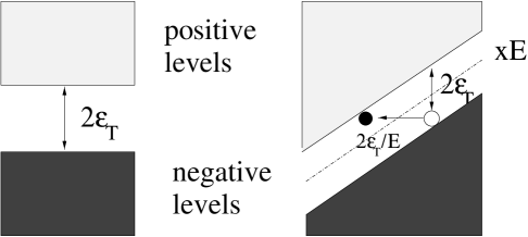
FIG. 1.: Left: For $E=0$ the vacuum is characterised by a completely filled negative-energy Dirac sea and an unoccupied positive-energy continuum, separated by a gap: $2\,\varepsilon_{\rm T}=2\,(m^{2}+p_{\perp}^{2})^{1/2}$. Right: Introducing a constant external field: $\vec{E}=\hat{e}_{x}E$, which is produced by a potential: $A^{0}=-E\vec{x}$, tilts the energy levels. In this case a particle in the negative-energy sea will tunnel through the gap with a probability $\sim\exp(-\pi\varepsilon_{T}^{2}/eE)$. Succeeding, it will be accelerated by the field in the $-x$-direction, while the hole it leaves behind will be accelerated in the opposite direction. The energy-level distortion is increased with increasing $E$ and hence so is the tunneling probability. $eE$ can be related to the flux-tube string-tension.

The production of charged particles leads naturally to an internal current. That current produces an electric field that increasingly screens and finally completely neutralises the background field so that particle creation stops. However, the current persists and the field associated with that internal current restarts the production process but now the field produced acts to retard and finally eliminate the current. …This is the back-reaction phenomenon and the natural consequences are time dependent fields and currents [9]. One observable and necessary consequence is plasma oscillations. Their properties, such as frequency and amplitude, depend on the initial strength of the background field and the frequency of interactions between the partons. It is clear that very frequent collisions will rapidly damp plasma oscillations and equilibrate the system.

The process we have described can be characterised by four distinct time-scales:

1. the quantum time, $\tau_{qu}$, which is set by the Compton wavelength of the particles produced and identifies the time-domain over which they can be localised/identified as “particles;”

2. the tunneling time, $\tau_{tu}$, which is inversely proportional to the flux tube field strength and describes the time between successive tunnelling events;

3. the plasma oscillation period, $\tau_{pl}$, which is also inversely proportional to field strength in the flux tube but is affected by other mechanisms as well;

4. and the collision period, $\tau_{coll}$, which is the mean time between two partonic collision events.

Each of the time-scales is important and the behaviour of the plasma depends on their relation to each other [10, 11]; e.g., non-Markovian (time-nonlocality) effects are dramatic if $\tau_{qu}\sim\tau_{tu}$. Herein we focus on the interplay of the larger time scales and consider a system for which $\tau_{pl}\sim\tau_{coll}$.

Particle creation is a natural outcome when solving QED in the presence of a strong external field and a formulation of this problem in terms of a kinetic equation is useful since, e.g., transport properties are easy to explore. The precise connection between this quantum kinetic equation and the mean field approximation in non-equilibrium quantum field theory [12] is not trivial and the derivation yields a kinetic equation that, importantly, is non-Markovian in character [13, 14, 15, 16].

The single particle distribution function is defined as the vacuum expectation value, in a time-dependent basis, of creation and annihilation operators for single particle states at time $t$ with three-momentum $\vec{p}$: $a^{\dagger}_{\vec{p}}(t)$, $a_{\vec{p}}(t)$; i.e.,

$$f(\vec{p},t):=\langle 0|a^{\dagger}_{\vec{p}}(t)\,a_{\vec{p}}(t)|0\rangle\,.$$ (2)

The evolution of this distribution function is described by the following quantum Vlasov equation:

$$\frac{df_{\pm}({\vec{P}},t)}{dt}=\frac{\partial f_{\pm}({\vec{P}},t)}{\partial t}+eE(t)\frac{\partial f_{\pm}({\vec{P}},t)}{\partial P_{\parallel}(t)}$$ (3)

$$= \frac{1}{2}{\cal W}_{\pm}(t)\int_{-\infty}^{t}dt^{\prime}{\cal W}_{\pm}(t^{\prime})\times[1\pm 2f_{\pm}({\vec{P}},t^{\prime})]\cos[x(t^{\prime},t)]+C_{\pm}({\vec{P}},t)\,,$$ (4)

where the lower [upper] sign corresponds to fermion [boson] pair creation, $C$ is a collision term and ${\cal W}_{\pm}$ are the transition amplitudes. The momentum is defined as ${\vec{P}}=(p_{1},p_{2},P_{\parallel}(t))$, with the longitudinal [kinetic] momentum $P_{\parallel}(t)=p_{3}-eA(t)$.

We approximate the collision-induced background field by an external, time-dependent, spatially homogeneous vector potential: $A_{\mu}$, in Coulomb gauge: $A_{0}=0$, taken to define the $z$-axis: ${\vec{A}}=(0,0,A(t))$. The corresponding electric field, also along the $z$-axis, is

$$E(t)=-{\dot{A}}(t)=-\frac{dA(t)}{dt}\,.$$ (5)

For fermions [13, 15] and bosons [11, 15] the transition amplitudes are

$${\cal W}_{-}(t)=\frac{eE(t)\varepsilon_{\perp}}{\omega^{2}(t)}\,,\;\;{\cal W}_{+}(t)=\frac{eE(t)P_{\parallel}(t)}{\omega^{2}(t)}\,,$$ (6)

where the transverse energy $\varepsilon_{\perp}=\sqrt{m^{2}+\vec{p}_{\perp}^{\,2}}$, $\vec{p}_{\perp}=(p_{1},p_{2})$, and $\omega(t)=\sqrt{\varepsilon_{\perp}^{2}+P_{\parallel}^{2}(t)}$ is the total energy. In Eq. (17),

$$x(t^{\prime},t)=2[\Theta(t)-\Theta(t^{\prime})]\,,\;\;\Theta(t)=\int^{t}_{-\infty}dt^{\prime}\omega(t^{\prime})\,,$$ (7)

is the dynamical phase difference.

The time dependence of the electric field is obtained by solving the Maxwell equation

$$-{\ddot{A}}^{\pm}(t)={\dot{E}}^{\pm}(t)=-j^{ex}(t)-j_{cond}(t)-j_{pol}(t)$$ (8)

where the three components of the current are: the external current generated, obviously, by the external field; the conduction current

$$j_{cond}(t)=g_{\pm}e\int\!\frac{d^{3}p}{(2\pi)^{3}}\,\frac{P_{\parallel}(t)}{\omega({\vec{P}},t)}f_{\pm}({\vec{P}},t)\,,$$ (9)

associated with the collective motion of the charged particles; and the polarisation current

$$j_{pol}(t)=g_{\pm}e\int\!\!\frac{d^{3}P}{(2\pi)^{3}}\frac{P_{\parallel}(t)}{\omega({\vec{P}},t)}\left[\frac{S({\vec{P}},t)}{{\cal W}_{\pm}({\vec{P}},t)}-\frac{e\,\dot{E}^{\pm}(t)\,P_{\parallel}(t)}{8\,\omega^{4}(\vec{P},t)}\right]\bigg{(}\frac{\epsilon_{\perp}}{P_{\parallel}(t)}\bigg{)}^{g_{\pm}-1}\!\!\!,$$ (10)

which is proportional to the production rate. Here $g_{-}=2$, $g_{+}=1$ and all fields and charges are understood to be fully renormalised, which has a particular impact on the polarisation current [17].

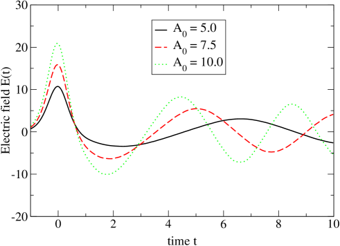
FIG. 2.: Time evolution of the fermion’s electric field obtained with three different initial field strengths. The amplitude and frequency of the plasma oscillations increases with an increase in the strength of the external impulse field, Eq. (11). The reference time-scale is the lifetime $b$ of the impulse current. (The field and time are given in arbitrary units, and $b=0.5$.)

We mimic a relativistic heavy ion collision by using an impulse profile for the external field

$$E_{ex}=-\frac{A_{0}}{b}{\rm sech}^{2}(t/b)\,,$$ (11)

which is our two-parameter model input: the width $b$ and the amplitude $A_{0}$ are chosen so that the initial conditions are comparable to typical/anticipated experimental values. This is the seed in a solution of the coupled system of Eqs. (17) and (8)–(10), and in Fig. 2 we illustrate the result for the electric field in the absence of collisions.

The qualitative features are obvious and easy to understand. The external impulse (the collision) is evident: the portion of the curve roughly symmetric about $t=0$, where the field assumes its maximum value $A_{0}/b$. It produces charged particles and accelerates them, producing a positive current and an associated field that continues to oppose the external field until the net field vanishes. At that time particle production ceases and the current reaches a maximum value. However, the external field is dying away: it’s lifetime is $t\sim 0.5$, so that the part of the electric field due to the particles’ own motion quickly finds itself too strong. The excess of field strength begins to produce particles. It accelerates these in the opposite direction to the particles generating the existing current whilst simultaneously decelerating the particles in that current. That continues until the particle current vanishes, at which point the net field has acquired its largest negative value. Particle production continues and with that a negative net current appears and grows. … Now a pattern akin to that of an undamped harmonic oscillator has appeared. In the absence of other effects, such as collisions, it continues in a steady state with the magnitude and period of the plasma oscillations determined by the two model parameters that characterise the collision.

The quantum kinetic equation, Eq. (17), describes a system far from equilibrium and therefore any realistic collision term $C$ valid shortly after the impact must be expected to have a very complex form. However, as Fig. 2 illustrates, the evolution at not-so-much later times is determined by the properties of the particles produced and not by the violent nonequilibrium effects of the collision. This observation suggests that the parton plasma can be treated as a quasi-equilibrium system and that the effects of collisions can be represented via a relaxation time approximation [17, 18, 19, 20, 21]:

$$C(\vec{p},t)=\frac{1}{\tau(t)}[f_{-}^{eq}(\vec{p},t)-f(\vec{p},t)]\,,$$ (12)

with $\tau(t)$ an in general time-dependent “relaxation time” (although we use a constant value $\tau(t)=\tau_{r}$ in the calculations reported herein) where

$$f_{-}^{eq}(\vec{p},T(t))=\left[\exp\left(\frac{p_{\nu}u^{\nu}(t)}{T(t)}\right)+1\right]^{-1}$$ (13)

is the quasi-equilibrium distribution function for fermions. Here $T(t)$ is a local-temperature and $u^{\nu}(t)$, $u^{2}=1$, is a hydrodynamical velocity [20]. (With our geometry, $u^{\nu}(t)=(1,0,0,v(t))/[1-v^{2}(t)]^{1/2}$.)

Our definition of quasi-equilibrium is to require that at each $t$ the energy and momentum density in the evolving plasma are the same as those in an equilibrated plasma; i.e., we require that

$$\epsilon_{f}(t)=\epsilon^{eq}(t)\,,\;\vec{p}_{f}(t)=\vec{p}^{\,eq}(t)$$ (14)

where, as one would expect,

$$\epsilon^{eq}(t)=\int\frac{d^{3}p}{(2\pi)^{3}}\,\omega(\vec{p},t)\,f_{-}^{eq}(\vec{p},t)\,,\;\vec{p}^{\,eq}(t)=\int\frac{d^{3}p}{(2\pi)^{3}}\,\vec{p}(t)\,f_{-}^{eq}(\vec{p},t)\,,$$ (15)

and

$$\epsilon_{f}(t) = \int\frac{d^{3}p}{(2\pi)^{3}}\,\omega(\vec{p},t)\left[f_{-}(\vec{p},t)-z_{f_{-}}(\vec{p},t)\right]\,,$$ (16)

$$\vec{p}_{f}(t) = \int\frac{d^{3}p}{(2\pi)^{3}}\,\vec{p}(t)\left[f_{-}(\vec{p},t)-z_{f_{-}}(\vec{p},t)\right]\,,$$ (17)

where

$$z_{f_{-}}(\vec{p},t)=\bigg{(}\frac{e\varepsilon_{\perp}}{4\omega^{3}}\bigg{)}^{2}\bigg{[}E(t)^{2}-\frac{e^{-2t/\tau_{r}}}{\tau_{r}}\int\limits_{-\infty}^{t}dt^{\prime}E(t^{\prime})^{2}e^{2t^{\prime}/\tau_{r}}\bigg{]}$$ (18)

is a regularising counterterm. Adding Eqs. (14) to the system of coupled equations embeds implicit equations for the temperature profile, $T(t)$, and collective velocity, $v(t)$.

Solving the complete set of coupled equations is a straightforward but time consuming exercise. For the present illustration we employ the minor simplification of assuming that the equilibrium energy density is that of a two-flavour, massless, free-quark gas; i.e.,

$$\epsilon^{eq}(T(t))=\frac{7\pi^{2}}{10}T^{4}(t)$$ (19)

and then proceed.

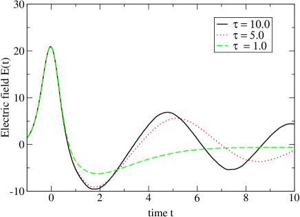
FIG. 3.: Time evolution of the electric field for three different relaxation times. As one would anticipate, collisions damp the plasma oscillations: their frequency and amplitude decreases with decreasing relaxation time. Solution obtained using the impulse profile, Eq. (11), with $A_{0}=10$, $b=0.5$. The field and the time are given in arbitrary units.

The solution obtained for the electric field using the impulse profile, Eq. (11), is depicted Fig. 3. Here the behaviour is analogous to that of a damped oscillator: the frequency and amplitude of the plasma oscillations diminishes with increasing collision frequency, $1/\tau_{r}$ (friction).

In the examples presented hitherto we have employed a constant fermion mass. However, in QCD the dressed-quark mass is momentum-dependent [22, 23] and that momentum-dependence is significant when $m_{0}\begin{picture}(1.4,1.0)\put(0.7,-0.3){\makebox(0.0,1.0)[t]{$<$}} \put(0.7,-0.3){\makebox(0.0,1.0)[b]{$\sim$}} \end{picture}\Lambda_{\rm QCD}$, where $m_{0}$ is the current-quark mass. That can be illustrated using a simple, instantaneous Dyson-Schwinger equation model of QCD, introduced in Ref. [24], which yields the following pair of coupled equations for the scalar functions in the dressed-quark propagator: $S(p)=1/[i\gamma\cdot p\,A(\vec{p}^{\,2})+B(\vec{p}^{\,2})]$,

$$B(\vec{p},t) = m_{0}+\eta\frac{B(\vec{p},t)}{\sqrt{\vec{p}^{2}\,A^{2}(\vec{p},t)+B^{2}(\vec{p},t)}}\,(1-2f_{-}(\vec{p},t))\,,$$ (20)

$$A(\vec{p},t) = \frac{2B(\vec{p},t)}{m_{0}+B(\vec{p},t)}\,,$$ (21)

where $\eta$ is the model’s mass scale. In this preliminary, illustrative calculation we discard the distribution function in Eq. (20).

The solution obtained using a current-quark mass $m_{0}=5\,$MeV and with $\eta=1.33\,$GeV is depicted in Fig. 4. This value of the mass-scale parameter can be compared with the potential energy in a QCD string at the confinement distance, $V_{q\bar{q}}(r=1\,\mbox{fm})=\sigma r\simeq(2\Lambda_{\rm QCD})^{2}(1/\Lambda_{\rm QCD})=4\Lambda_{\rm QCD}\sim 1.0\,$GeV. The dressed-quark mass function is $m(\vec{p}^{\,2},T)=B(\vec{p}^{\,2},T)/A(\vec{p}^{\,2},T)$, and $m(0,T)$ provides a practical estimate of the $T$-dependent constituent-quark mass [26]: in this example $m(0,T_{c})\approx 0.35\,$GeV.

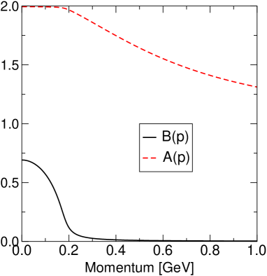
FIG. 4.: The scalar functions characterising a dressed-$u$-quark propagator, as function of momentum, obtained using the simple DSE model introduced in Ref. [24], see Eqs. (20), (21). We plot the functions as obtained at $T=T_{c}=0.17\,$GeV, which is the critical temperature for deconfinement in the model [25].

In our flux tube model for particle production we produce fermions with different momenta and following this discussion it is clear that the effective mass of the particles produced must be different for each momentum. That will affect the production and evolution of the plasma. To illustrate that we have repeated the last calculation using $m(p)$ wherever the particle mass appears in the system of coupled equations for the single particle distribution function. The effect on the electric field is depicted in Fig. 5, wherein it is evident that the plasma oscillation frequency is increased when the momentum-dependent mass is used because many of the particles produced are now lighter than the reference mass and hence respond more quickly to changes in the electric field.

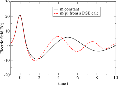
FIG. 5.: Electric field as function of time for $A_{0}=10.0$, $\tau=5.0$, $b=0.5$. We compare the results obtained using particles produced with a constant mass, $m=1$, with those obtained when the mass is momentum-dependent. For illustrative simplicity, we use the profile in Fig. 4 but normalised such that, $m(0)=m$. The mass-scale is arbitrary.

We have sketched a quantum Vlasov equation approach to the study of particle creation in strong fields. Using a simple model to mimic a relativistic heavy ion collision, we solved for the single particle distribution function and the associated particle currents and electric fields. Plasma oscillations are a necessary feature of all such studies. We illustrated that the oscillation frequency depends on: the initial energy density reached in the collision, it increases with increasing energy density; and the particle-particle collision probability, it decreases as this probability increases; and that it is sensitive to the necessary momentum-dependence of dressed-particle mass functions. The response in each case is easy to understand intuitively and that is a strength of the Vlasov equation approach.

Acknowledgments. A.V.P. is grateful for financial support provided by the Deutsche Forschungsgemeinschaft under project no. 436 RUS $17/102/00$. This work was supported by the US Department of Energy, Nuclear Physics Division, under contract no. W-31-109-ENG-38; the US National Science Foundation under grant no. INT-9603385; and benefited from the resources of the National Energy Research Scientific Computing Center.

Kinetic Equilibration of Gluons in High-Energy Heavy Ion Collisions

J. Serreau

LPT, Bâtiment 210, Université Paris-Sud,
91405 Orsay, France

A Introduction

A central question in the study of high-energy heavy ion collision is that of the possible formation and thermalization of a deconfined state of matter, the quark-gluon plasma (QGP). It is widely believed that a large amount of gluons with transverse momentum $p_{t}\sim 1-2$ GeV are produced in the very early stages of such collisions [1, 2]. Wether this dense gas of partons thermalizes before hadronization is a question of great interest for interpreting the data at RHIC and LHC. So far, most of the predictions concerning QGP signatures rely on the assumption that the system is at least in kinetic equilibrium.

It is widely assumed in the literature (see e.g. [3]) that elastic collisions between partons, which randomize their momenta, rapidly drive the system toward kinetic equilibrium, on time scales $\lesssim 1$ fm (see e.g. [4]). It was argued however that, due to the effect of longitudinal expansion at early times, at least elastic collisions may not be effective enough [5]. Also, the emphasis was put on the importance of the initial condition which characterizes the partonic system just after the collision [2, 6]. The purpose of the work reported here is to examine this question again. We consider only gluons and assume that already at early times a local Boltzmann equation can be written for the partonic phase space distribution. We include only $2\rightarrow 2$ elastic processes in the small-scattering angle limit and work in the relaxation time approximation. We compare the case where initial conditions are given by the saturation scenario (see [2]), to the case where the initial gluons are produced incoherently in semi-hard (perturbative) processes, the so-called minijet scenario [1]. By consistently including the effect of collisions in the calculation of the relaxation time, we reproduce semi-qualitative features of the exact solution of the Boltzmann equation, recently obtained numerically in [7]. We follow the approach toward kinetic equilibrium by testing the isotropy of different observables. This way of characterizing equilibration is more satisfying than that used in [7], and leads to different conclusions. In particular, we find that, in both scenarios, the system does not equilibrate at RHIC energies. More generally, we show that the assumption that elastic collisions are efficient enough to rapidly achieve kinetic equilibrium is not reliable. Due to the longitudinal expansion, the actual kinetic equilibration time is an order of magnitude bigger than the typical $1$ fm estimate usually assumed.

In Section B we present the model used to describe the time evolution of the local partonic distribution in the central region of the collision. We describe in particular the method we use to compute “self-consistently” the relaxation time. The results of our analysis of kinetic equilibration in the saturation and minijet scenarios are presented in Section C. More details about the work presented here can be found in [8].

B The model

Shortly after being produced, because of the expansion, the parton system is rapidly diluted enough so one can reliably describe it as a gas of classical particles. One can then use a classical Boltzmann equation to describe the time evolution of the local phase-space distribution $f(\vec{p},\vec{x},t)$: $df/dt={\mathcal{C}}$, where ${\mathcal{C}}$ is the collision integral. Here we consider only elastic $gg\rightarrow gg$ scatterings in the small-angle limit. Assuming one-dimensional expansion at early times and longitudinal boost invariance in the central region of the collision ($z\simeq 0$) in the center of mass frame, one obtains a simple equation at constant $p_{z}t$. It reads, in the leading logarithmic approximation for the collision term [9, 2],

$$\left.\partial_{t}f(\vec{p},t)\right|_{p_{z}t}={\mathcal{L}}\,N_{0}\nabla_{p}^{2}f(\vec{p},t)+2{\mathcal{L}}\,N_{-1}\vec{\nabla}_{p}\left[\vec{v}\,f(\vec{p},t)\right]\,,$$ (1)

where $\vec{v}=\vec{p}/p$, and where ${\mathcal{L}}=2\pi\alpha_{S}^{2}\frac{N_{c}^{2}}{N_{c}^{2}-1}\,\int d\chi/\chi$ is a logarithmically divergent integral which is physically regulated by medium effects (see for example [7] and references therein). We have defined the moments $N_{s}=\langle p^{s}\rangle=\int_{\vec{p}}\,p^{s}\,f(\vec{p},t)$, with the notation $\int_{\vec{p}}\,\equiv\,2(N_{c}^{2}-1)\int d^{3}p/(2\pi)^{3}$.

The Boltzmann equation (1) has been numerically solved in the saturation scenario in Ref. [7]. Here we solve the equations for moments of the distribution in a relaxation time approximation (RTA), taking into account “self-consistently” the dynamical information contained in (1). The RTA consists in replacing the collision term of the Boltzmann equation by an exponential relaxation term [11]:

$$\left.\partial_{t}f\right|_{p_{z}t=\mbox{cte}}\equiv-(f-f_{eq})/\theta\,,$$ (2)

with $f_{eq}(\vec{p},t)=\lambda(t)\,\exp(-p/T(t))$. The parameters $\lambda$ and $T$ are determined at each time by using the conservation of energy and of particle number in elastic collisions. In the RTA, these leads to the following equations for the energy and particle number densities per unit volume $\epsilon=N_{1}$ and $n=N_{0}$:

$$\epsilon(t) = \epsilon_{eq}(t)=6\frac{N_{c}^{2}-1}{\pi^{2}}\,\lambda(t)\,T^{4}(t)\,,$$ (3)

$$n(t) = n_{eq}(t)=2\frac{N_{c}^{2}-1}{\pi^{2}}\,\lambda(t)\,T^{3}(t)\,.$$ (4)

We stress here that the time-dependent parameter $\lambda(t)$ is needed in order to enforce particle number conservation (which gives the exact equation $t\,n(t)=$ cte) and energy conservation independently. Also it is important to note that the parameter $T(t)$ does not have the physical meaning of a local temperature unless the system has reached the hydrodynamic regime (where $\lambda=$cte and $t^{1/3}T=$cte [12]).

The third parameter of the RTA ansatz, namely the relaxation time $\theta$, contains the dynamical information about the collisions. For simplicity, we assume it to be momentum-independent. To compute $\theta$, we shall identify the r.h.s of Eqs. (1) and (2). This cannot be done directly and one has instead to identify some moment of these r.h.s:

$$\int_{\vec{p}}\,m(\vec{p})\,{\mathcal{C}}(\vec{p},t)=-\frac{\langle m\rangle(t)-\langle m\rangle_{eq}(t)}{\theta_{m}(t)}\,,$$ (5)

where $m(\vec{p})$ is an arbitrary function, $\langle m\rangle_{(eq)}=\int_{\vec{p}}\,m(\vec{p})\,f_{(eq)}(\vec{p},t)$, and $\theta_{m}(t)$ is the associated relaxation time. Being interested in kinetic equilibration, that is in the relaxation of the momentum distribution of the typical particles of the system toward isotropy, we choose $m$ so that it picks up the corresponding momentum scale in the distribution, and then the relevant relaxation time. The momentum scale we are interested in is that of the particles which build the “thermodynamic” quantities, like the energy density, or the longitudinal and transverse pressure densities $P_{L}=\langle p_{z}^{2}/p\rangle$ and $P_{T}=\langle p_{\perp}^{2}/p\rangle$, where $p_{\perp}^{2}=(p_{x}^{2}+p_{y}^{2})/2$. A pertinent choice leading to simple equations is $\langle m\rangle=P_{L}-P_{T}$. Using Eqs. (1) and (5), one obtains the following equation for $\theta(t)$:

$$\frac{N_{1}^{z}-N_{1}^{\perp}}{\theta}=4\,{\mathcal{L}}\,N_{0}\,(N_{-1}^{z}-N_{-1}^{\perp})+2\,{\mathcal{L}}\,N_{-1}\,(N_{0}^{z}-N_{0}^{\perp})\,,$$ (6)

where we defined $N_{s}^{z}=\langle p_{z}^{2}\,p^{s-2}\rangle$ and $N_{s}^{\perp}=\langle p_{\perp}^{2}\,p^{s-2}\rangle$. For a particular choice of initial distribution, we solve Eqs. (2), (3), (4) and (5) numerically (for details see [8]). We can then follow the system toward kinetic equilibrium by measuring the isotropy of different observables.

C Kinetic equilibration

Here we present results for two different initial conditions relevant to high energy nuclear collisions at RHIC and LHC: the saturation and minijet scenarios. In both cases we use the distributions proposed in the literature, which we recall below (see the corresponding references for details).

  - Saturation scenario:

the initial distribution has the form [2, 7]

$$f_{0}(\vec{p})=f_{sat}(\vec{p},t_{0})=\frac{c}{\alpha_{S}N_{c}}\,\delta(p_{z})\,\Theta(Q_{s}^{2}-p_{t}^{2})\,$$

where $t_{0}$ is the initial time, $Q_{s}$ is the saturation momentum and $c\sim 1$ is a numerical constant. The values of these parameters corresponding to RHIC and LHC energies are taken from [7]: $c\simeq 1.3$, $t_{0}=0.4\,(0.18)$ fm and $Q_{s}=1\,(2)$ GeV at RHIC (LHC).

  - Minijet scenario:

the initial distribution has the form [10]

$$f_{0}(\vec{p})=f_{jet}(\vec{p},t_{0})=\exp(-p/T_{jet})\,,$$

the parameter $T_{jet}$ being determined from the initial energy and particle number densities. One has $t_{0}=0.18\,(0.09)$ fm and $T_{jet}=0.535\,(1.13)$ GeV at RHIC (LHC).

In each case we measure the anisotropy of the distribution by means of the ratios $R_{k}=N_{k}^{z}/N_{k}^{\perp}$ of longitudinal and transverse moments, which should approach $1$ as the gas equilibrates. We stop the time evolution when the particle number density becomes less than $n_{c}=1$/fm³, after which the partonic description becomes meaningless. In both scenarios, the corresponding time is $t_{max}\approx 10$ fm at RHIC and $t_{max}\approx 30$ fm at LHC. Although our approximation of longitudinally boost-invariant geometry can only hold for times $\lesssim R$, where $R\sim 5$ fm is the transverse size of the system (the radius of the incident nuclei), we present the results for $t\leq t_{max}$ in order to show how the system behaves. The solid curves in Figs. 1 and 2 show the time evolution of the ratio $R_{1}=P_{L}/P_{T}$ at RHIC and LHC energies for the saturation and minijet scenario respectively, where we took $\alpha_{S}=0.3$. We stress here that the results obtained in the RTA are in good agreement with the exact solution obtained in [7] in the saturation scenario.

FIG. 1.: Time evolution of the ratio of longitudinal and transverse pressures in the saturation scenario at RHIC and LHC. The solid curve corresponds to the choice $\alpha_{S}=0.3$. The upper (lower) curves are obtained by multiplying (dividing) the collision integral $\mathcal{C}$ by a factor $2$. This gives a rough estimate of the uncertainties of our simple description.

FIG. 2.: The same as Fig. 1 for the minijet scenario.

In order to estimate roughly the uncertainties of our description, in particular those related to the choice of $\alpha_{S}$ and to the details of the screening of the logarithmically divergent integral $\mathcal{L}$ (see above), we simply multiply and divide the collision integral by $2$. These respectively result in the dotted and dashed curves of Figs. 1 and 2. We see in both scenarios that, at RHIC energy, the distribution is still far from being isotropic ($P_{L}/P_{T}\lesssim 0.8$), even for $t\sim 10$ fm. At LHC, for $t\sim 10$ fm, although the saturation scenario seems more favorable, no conclusion can be made because of the uncertainties of our description. What can be said however is that the typical equilibration time is at least of the order of a few fermis. This contradicts the usual assumption that elastic collisions are sufficient to achieve kinetic equilibrium on very short ($\lesssim 1$ fm) time-scales.

D Conclusion

We studied the kinetic equilibration of the gluon gas produced in the very early times of a very high energy heavy ion collision. We studied in particular two different types of initial state relevant to these collisions: the saturation and minijet scenarios. Assuming that, already at early times, the system can be described by a classical Boltzmann equation for the local partonic phase-space distribution, we investigate the role of $2\rightarrow 2$ processes by using a relaxation time approximation. By measuring the anisotropy of different observables, we can follow the system towards kinetic equilibrium. Our results show that elastic collisions are not as efficient as usually believed to achieve kinetic equilibration: because of the effect of longitudinal expansion in the early stages, the typical equilibration time is of the order of a few fermis, which is comparable to the typical life-time of the partonic system.

Photoproduction of Charmonia and Total Charmonium-Proton Cross Sections

J. Hüfner^a,b, Yu.P. Ivanov^a,b,c, B.Z. Kopeliovich^b,c and A.V. Tarasov^a,b,c

^a Institut für Theoretische Physik der Universität, Germany
^b Max-Planck Institut für Kernphysik, Germany
^c Joint Institute for Nuclear Research, Dubna, Russia

A Introduction

The dynamics of production and interaction of charmonia has drawn attention since their discovery back in 1973. As these heavy mesons have a small size it has been expected that hadronic cross sections may be calculated relying on perturbative QCD. The study of charmonium production became even more intense after charmonium suppression had been suggested as a probe for the creation and interaction of quark-gluon plasma in relativistic heavy ion collisions [1]. Since we will never have direct experimental information on charmonium-nucleon total cross sections one has to extract it from other data for example from elastic photoproduction of charmonia $\gamma p\to J\!/\!\psi(\psi^{\prime})\ p\,$. The widespread believe that one can rely on the vector dominance model (VDM) is based on previous experience the with photoproduction of $\rho$ mesons but fails badly for charmonia.

Instead, one may switch to the quark basis, which should be equivalent to the hadronic basis because of completeness. In this representation the procedure of extracting $\sigma^{J\!/\!\psi\,p}_{tot}$ from photoproduction data cannot be realized directly, but has to be replaced by a different strategy. Namely, as soon as one has expressions for the wave functions of charmonia and the universal dipole cross section $\sigma_{q\bar{q}}(r_{T},s)$, one can predict both, the experimentally known charmonium photoproduction cross sections and the unknown $\sigma^{J\!/\!\psi(\psi^{\prime})\,p}_{tot}$. If the photoproduction data are well described one may have some confidence in the predictions for the $\sigma^{J\!/\!\psi(\psi^{\prime})p}_{tot}$.

In the light-cone dipole approach the two processes, photoproduction and charmonium-nucleon elastic scattering look as shown in Fig. 1 [2].

  

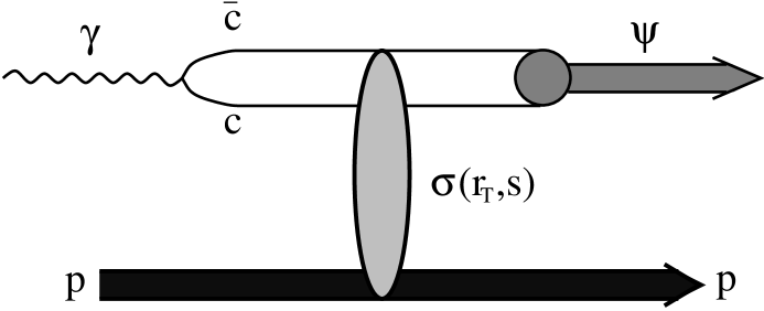
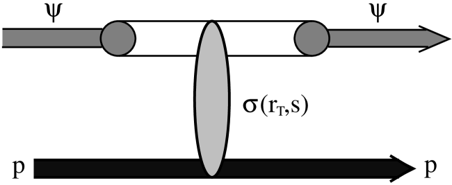
FIG. 1.: Schematic representation of the amplitudes for the reactions $\gamma^{*}p\to\psi p$ (left) and $\psi\,p$ elastic scattering (right) in the rest frame of the proton. The $c\bar{c}$ fluctuation of the photon and the $\psi$ with transverse separation $r_{T}$ and c.m. energy $\sqrt{s}$ interact with the target proton via the cross section $\sigma(r_{T},s)$ and produce a $J\!/\!\psi$ or $\psi^{\prime}$.

The corresponding expressions for the forward amplitudes read

$${\cal M}_{\gamma^{*}p}(s,Q^{2}) = \sum_{\mu,\bar{\mu}}\,\int\limits_{0}^{1}\!\!d\alpha\!\int\!\!d^{2}{\vec{r}_{T}}\,\Phi^{\!*(\mu,\bar{\mu})}_{\psi}(\alpha,{\vec{r}_{T}})\,\sigma_{q\bar{q}}(r_{T},s)\,\Phi^{(\mu,\bar{\mu})}_{\gamma^{*}}(\alpha,{\vec{r}_{T}},Q^{2})$$ (1)

$${\cal M}_{\psi\,p}(s) = \sum_{\mu,\bar{\mu}}\,\int\limits_{0}^{1}\!\!d\alpha\!\int\!\!d^{2}{\vec{r}_{T}}\,\Phi^{\!*(\mu,\bar{\mu})}_{\psi}(\alpha,{\vec{r}_{T}})\,\sigma_{q\bar{q}}(r_{T},s)\,\Phi^{(\mu,\bar{\mu})}_{\psi}(\alpha,{\vec{r}_{T}})\ .\left.~{}~{}\right.$$ (3)

Here the summation runs over spin indexes $\mu$, $\bar{\mu}$ of the $c$ and $\bar{c}$ quarks, $Q^{2}$ is the photon virtuality, $\Phi_{\gamma^{*}}(\alpha,r_{T},Q^{2})$ is the light-cone distribution function of the photon for a $c\bar{c}$ fluctuation of separation $r_{T}$ and relative fraction $\alpha$ of the photon light-cone momentum carried by $c$ or $\bar{c}$. Correspondingly, $\Phi_{\psi}(\alpha,{\vec{r}_{T}})$ is the light-cone wave function of $J\!/\!\psi$, $\psi^{\prime}$ and $\chi$ (only in Eq. 3). The dipole cross section $\sigma_{q\bar{q}}(r_{T},s)$ mediates the transition (cf Fig. 1). We discuss the various ingredients.

B Light-cone dipole formalism

The light cone variable describing longitudinal motion which is invariant to Lorentz boosts is the fraction $\alpha=p_{c}^{+}/p_{\gamma^{*}}^{+}$ of the photon light-cone momentum $p_{\gamma^{*}}^{+}=E_{\gamma^{*}}+p_{\gamma^{*}}$ carried by the quark or antiquark. In the nonrelativistic approximation (assuming no relative motion of $c$ and $\bar{c}$) $\alpha=1/2$ (e.g. [2]), otherwise one should integrate over $\alpha$ (see Eq. (1)). For transversely ($T$) and longitudinally ($L$) polarized photons the perturbative photon-quark distribution function in Eq. (1) reads [3, 4],

$$\Phi_{T,L}^{(\mu,\bar{\mu})}(\alpha,{\vec{r}_{T}},Q^{2})=\frac{\sqrt{N_{c}\,\alpha_{em}}}{2\,\pi}\,Z_{c}\,\chi_{c}^{\mu\dagger}\,\widehat{O}_{T,L}\,\widetilde{\chi}_{\bar{c}}^{\bar{\mu}}\,K_{0}(\epsilon r_{T})\ ,$$ (4)

where

$$\widetilde{\chi}_{\bar{c}}=i\,\sigma_{y}\,\chi^{*}_{\bar{c}}\ ;$$ (5)

$\chi$ and $\bar{\chi}$ are the spinors of the $c$-quark and antiquark respectively, $\widehat{O}_{T,L}$ are operators acting on the spin, $Z_{c}=2/3$. $K_{0}(\epsilon r_{T})$ is the modified Bessel function with

$$\epsilon^{2}=\alpha(1-\alpha)Q^{2}+m_{c}^{2}\ .$$ (6)

1 Phenomenological dipole cross section

The dipole formalism for hadronic interactions introduced in [5] expands the hadronic cross section over the eigen states of the interaction which in QCD are the dipoles with a definite transverse separation (see (1)). Correspondingly, the values of the dipole cross section $\sigma_{q\bar{q}}(r_{T})$ for different $r_{T}$ are the eigenvalues of the elastic amplitude operator. This cross section is flavor invariant, due to universality of the QCD coupling, and vanishes like $\sigma_{q\bar{q}}(r_{T})\propto r^{2}_{T}$ for $r_{T}\!\!\to\!0$. The latter property is sometimes referred to as color transparency.

The total cross sections for all hadrons and (virtual) photons are known to rise with energy. Apparently, the energy dependence cannot originate from the hadronic wave functions in Eqs. (1, 3), but only from the dipole cross section. In the approximation of two-gluon exchange used in [5] the dipole cross section is constant, the energy dependence originates from higher order corrections related to gluon radiation. On the other way, one can stay with two-gluon exchange, but involve higher Fock states which contain gluons in addition to the $q\bar{q}$. Both approaches correspond to the same set of Feynman graphs. We prefer to introduce energy dependence into $\sigma_{q\bar{q}}(r_{T},s)$ and not include higher Fock states into the wave functions.

Since no reliable way to sum up higher order corrections is known so far, we use a phenomenological form which interpolates between the two limiting cases of small and large separations. Few parameterizations are available in the literature, we choose two of them which are simple, but quite successful in describing data and denote them by the initials of the authors as “GBW” [6] and “KST” [7] and give the explicit expression for KST:

$$\mbox{``KST'':}~{}~{}~{}~{}~{}~{}~{}~{}~{}\sigma_{\bar{q}q}(r_{T},s) = \sigma_{0}(s)\left[1-e^{-r_{T}^{2}/r_{0}^{2}(s)}\right]\ .~{}~{}~{}~{}~{}~{}$$ (7)

The values and energy dependence of hadronic cross sections is guaranteed by the choice of

$$\sigma_{0}(s) = 23.6\left(\frac{s}{s_{0}}\right)^{\!\!0.08}\left(1+\frac{3}{8}\frac{r_{0}^{2}(s)}{\left<r^{2}_{ch}\right>}\right)\,\mbox{mb}\ ,$$ (8)

$$r_{0}(s) = 0.88\left(\frac{s}{s_{0}}\right)^{\!\!-0.14}\,\mbox{fm}\ .$$ (9)

The energy dependent radius $r_{0}(s)$ is fitted to data for the proton structure function $F^{p}_{2}(x,Q^{2})$, $s_{0}=1000\,\mbox{GeV}^{2}$ and the mean square of the pion charge radius $\left<r^{2}_{ch}\right>=0.44\,\mbox{fm}^{2}$. The improvement at large separations leads to a somewhat worse description of the proton structure function at large $Q^{2}$. Apparently, the cross section dependent on energy, rather than $x$, cannot provide Bjorken scaling. Indeed, parameterization (7) is successful only up to $Q^{2}\approx 10\,\mbox{GeV}^{2}$.

2 Charmonium wave functions

The spatial part of the $c\bar{c}$ pair wave function satisfying the Schrödinger equation

$$\left(-\,\frac{\Delta}{m_{c}}+V(r)\right)\,\Psi_{nlm}(\vec{r}\,)=E_{nl}\,\Psi_{nlm}(\vec{r}\,)$$ (10)

is represented in the form

$$\Psi(\vec{r}\,)=\Psi_{nl}(r)\cdot Y_{lm}(\theta,\varphi)\ ,$$ (11)

where $\vec{r}\,$ is 3-dimensional $c\bar{c}$ separation, $\Psi_{nl}(r)$ and $Y_{lm}(\theta,\varphi)$ are the radial and orbital parts of the wave function. The equation for radial $\Psi(r)$ is solved with the help of the program [8]. Four different potentials $V(r)$ have been used (“BT” [9], “COR” [10], “LOG” [11] and “POW” [12]), of which we give one example (“COR” - Cornell potential [10]):

$$V(r)=-\frac{k}{r}+\frac{r}{a^{2}}$$ (12)

with $k=0.52$, $a=2.34\,\mbox{GeV}^{-1}$ and $m_{c}=1.84\,\mbox{GeV}$.

The results of calculations for the radial part $\Psi_{nl}(r)$ of the $1S$ and $2S$ states are depicted in Fig. 2. For the ground state all the potentials provide a very similar behavior for $r>0.3\,\mbox{fm}$, while for small $r$ the predictions differ by up to $30\%$. The peculiar property of the $2S$ state wave function is the node at $r\approx 0.4\,\mbox{fm}$ which causes strong cancelations in the matrix elements Eq. (1) and as a result, a suppression of photoproduction of $\psi^{\prime}$ relative to $J\!/\!\psi$ [2, 13].

  

FIG. 2.: The radial part of the wave function $\Psi_{nl}(r)$ for the $1S$ and $2S$ states calculated with four different potentials (see text).

3 Light-cone wave functions for the bound states

As has been mentioned, the lowest Fock component $|c\bar{c}\rangle$ in the infinite momentum frame is not related by simple Lorentz boost to the wave function of charmonium in the rest frame. This makes the problem of building the light-cone wave function for the lowest $|c\bar{c}\rangle$ component difficult, no unambiguous solution is yet known. There are only recipes in the literature, a simple one widely used [14], is the following. One applies a Fourier transformation from coordinate to momentum space to the known spatial part of the non-relativistic wave function (11), $\Psi(\vec{r}\,)\Rightarrow\Psi(\vec{p}\,)$, which can be written as a function of the effective mass of the $c\bar{c}$, $M^{2}=4(p^{2}+m_{c}^{2})$, expressed in terms of light-cone variables

$$M^{2}(\alpha,p_{T})=\frac{p_{T}^{2}+m_{c}^{2}}{\alpha(1-\alpha)}\ .$$ (13)

In order to change integration variable $p_{L}$ to the light-cone variable $\alpha$ one relates them via $M$, namely $p_{L}=(\alpha-1/2)M(p_{T},\alpha)$. In this way the $c\bar{c}$ wave function acquires a kinematical factor

$$\Psi(\vec{p}\,)\Rightarrow\sqrt{2}\,\frac{(p^{2}+m_{c}^{2})^{3/4}}{(p_{T}^{2}+m_{c}^{2})^{1/2}}\cdot\Psi(\alpha,{\vec{p}_{T}})\equiv\Phi_{\psi}(\alpha,{\vec{p}_{T}})\ .$$ (14)

This procedure is used in [15] and the result is applied to calculation of the amplitudes (1). This leads to the enhancement of $\Psi^{\prime}$ photoproduction.

The 2-dimensional spinors $\chi_{c}$ and $\chi_{\bar{c}}$ describing $c$ and $\bar{c}$ respectively in the infinite momentum frame are known to be related via the Melosh rotation [16, 14] to the spinors $\bar{\chi}_{c}$ and $\bar{\chi}_{\bar{c}}$ in the rest frame:

$$\bf\overline{\chi}_{c} = \widehat{R}(\alpha,{\vec{p}_{T}})\,\chi_{c}\ ,$$ (15)

$$\bf\overline{\chi}_{\bar{c}} = \widehat{R}(1-\alpha,-{\vec{p}_{T}})\,\chi_{\bar{c}}\ ,$$ (16)

where the matrix $R(\alpha,{\vec{p}_{T}})$ has the form:

$$\widehat{R}(\alpha,{\vec{p}_{T}})=\frac{m_{c}+\alpha\,M-i\,[\vec{\sigma}\times\vec{n}]\,{\vec{p}_{T}}}{\sqrt{(m_{c}+\alpha\,M)^{2}+p_{T}^{2}}}\ .$$ (17)

Since the potentials we use in section B 2 contain no spin-orbit term, the $c\bar{c}$ pair is in $S$-wave. In this case spatial and spin dependences in the wave function factorize and we arrive at the following light cone wave function of the $c\bar{c}$ in the infinite momentum frame

$$\Phi^{(\mu,\bar{\mu})}_{\psi}(\alpha,{\vec{p}_{T}})=U^{(\mu,\bar{\mu})}(\alpha,{\vec{p}_{T}})\cdot\Phi_{\psi}(\alpha,{\vec{p}_{T}})\ ,$$ (18)

where

$$U^{(\mu,\bar{\mu})}(\alpha,{\vec{p}_{T}})=\chi_{c}^{\mu\dagger}\,\widehat{R}^{\dagger}(\alpha,{\vec{p}_{T}})\,\vec{\sigma}\cdot\vec{e}_{\psi}\,\sigma_{y}\,\widehat{R}^{*}(1-\alpha,-{\vec{p}_{T}})\,\sigma_{y}^{-1}\,\widetilde{\chi}_{\bar{c}}^{\bar{\mu}}$$ (19)

and $\widetilde{\chi}_{\bar{c}}$ is defined in (5). The Melosh rotation is extremely important and changes the calculations for photo production by up to a factor two.

C Calculations and comparison with data

1 $s$ and $Q^{2}$ dependence of $\sigma(\gamma^{*}p\to J\!/\!\psi\,p$)

Now we are in a position to calculate the cross section of charmonium photoproduction

$$\sigma_{\gamma^{*}p\to\psi p}(s,Q^{2})=\frac{|\widetilde{\cal M}_{T}(s,Q^{2})|^{2}+\varepsilon\,|\widetilde{\cal M}_{L}(s,Q^{2})|^{2}}{16\,\pi\,B}\ ,$$ (20)

where $\varepsilon$ is the photon polarization (for H1 data $\langle\varepsilon\rangle=0.99$) and $B=4.73\,GeV^{-2}$ is the slope parameter in reaction $\gamma^{*}p\to\psi p$ [17]. $\widetilde{\cal M}_{T,L}$ includes also the correction for the real part of the amplitude:

$$\widetilde{\cal M}_{T,L}(s,Q^{2})={\cal M}_{T,L}(s,Q^{2})\,\left(1-i\,\frac{\pi}{2}\,\frac{\partial\,\ln{\cal M}_{T,L}(s,Q^{2})}{\partial\,\ln s}\right)\ .$$ (21)

The results for $J/\psi$ are compared with the data in Fig. 3.

FIG. 3.: Integrated cross section for elastic photoproduction $\gamma\,p\rightarrow J/\psi\,p$ with real photons ($Q^{2}=0$) as a function of the energy calculated with GBW and KST dipole cross sections and for four potentials to generate $J\!/\!\psi$ wave functions. Experimental data points from the H1 [17], E401 [18], E516 [19] and ZEUS [20] experiments.

Calculations are performed with GBW and KST parameterizations for the dipole cross section and for wave functions of the $J\!/\!\psi$ calculated from BT, LOG, COR and POW potentials. One observes

• There are no major differences for the results using the GBW and KST parameterizations.

• The use of different potentials to generate the wave functions of the $J\!/\!\psi$ leads to two distinctly different behaviors. The potentials labeled BT and LOG (see sect. B 2) describe the data very well, while the potentials COR and LOG underestimate them by a factor of two. The different behavior has been traced to the following origin: BT and LOG use $m_{c}\approx 1.5\,\mbox{GeV}$, but COR and POW $m_{c}\approx 1.8\,\mbox{GeV}$. While the bound state wave functions of $J\!/\!\psi$ are little affected by this difference (see Fig. 2), the photon wave function Eq. (4) depends sensitively on $m_{c}$ via the argument Eq. (6) of the $K_{0}$ function.

  We compare our calculations also with data for the $Q^{2}$ dependence of the cross section. The data are plotted in Fig. 4 at c.m. energy $\sqrt{s}=90\,\mbox{GeV}$ as a function of $Q^{2}+M^{2}_{J\!/\!\psi}$, since in this form both, data and calculations display an approximate power law dependence. Such a dependence on $Q^{2}+M^{2}_{J\!/\!\psi}$ is suggested by the variable $\epsilon^{2}$ in Eq. (6), which for $\alpha=1/2$ takes the value $Q^{2}+(2\,m_{c})^{2}$. It may be considered as an indication that $\alpha=1/2$ is a reasonable approximation for the nonrelativistic charmonium wave function.

FIG. 4.: Integrated cross section for elastic photo production as a function of the photon virtuality $Q^{2}+M_{J/\psi}$ at energy $\sqrt{s}=90\,\mbox{GeV}$. Solid and dashed curves are calculated with GBW and KST dipole cross sections, while thick and thin curves correspond to BT and COR potentials, respectively. Results obtained with LOG and POW potentials are very close to that curves (LOG similar to BT and POW to COR, see also Fig. 3).

Our results are depicted for BT and COR potentials and using GBW and KST cross sections. Agreement with the calculations based on BT potential is again quite good, while the COR potential grossly underestimate the data at small $Q^{2}$. Although the GBW and KST dipole cross sections lead to nearly the same cross sections for real photoproduction, their predictions at high $Q^{2}$ are different by a factor $2-3$. Supposedly the GBW parameterization should be more trustable at $Q^{2}\gg M_{\Psi}^{2}$.

2 Importance of spin effects for the $\psi^{\prime}$ to $J\!/\!\psi$ ratio

It turns out that the effects of spin rotation have a gross impact on the cross section of elastic photoproduction $\gamma\,p\to J\!/\!\psi(\psi)p\,$. We see that these effects add 30-40% to the $J\!/\!\psi$ photoproduction cross section.

The spin rotation effects turn out to have a much more dramatic impact on $\psi^{\prime}$ increasing the photoproduction cross section by a factor 2-3. This spin effects explain the large values of the ratio $R$ observed experimentally. Our results for $R$ are about twice as large as evaluated in [21] and even more than in [15].

The ratio of $\psi^{\prime}$ to $J\!/\!\psi$ photoproduction cross sections is depicted as function of c.m. energy in Fig. 5. Our calculations agree with available data, but error bars are too large to provide a more precise test for the theory. Remarkably, the ratio $R(s)$ rises with energy.

FIG. 5.: The ratio of $\psi^{\prime}$ to $J/\psi$ photoproduction cross sections as a function of c.m. energy calculated for all four potentials with with GBW and KST parameterizations for the dipole cross section. Experimental data points from the SLAC [22], NA14 [23], E401 [24], EMC [25], NMC [26] and H1 [27] experiments.

D Charmonium-nucleon total cross sections

After the light-cone formalism has been checked with the data for virtual photoproduction we are in position to provide reliable predictions for charmonium-nucleon total cross sections. The calculated $J\!/\!\psi$- and $\psi^{\prime}$-nucleon total cross sections are plotted in Fig. 6 for the GBW and KST forms of the dipole cross sections and all four types of the charmonium potentials.

FIG. 6.: Total $J\!/\!\psi\,p$ (thick curves) and $\psi^{\prime}\,p$ (thin curves) cross sections with the GBW and KST parameterizations for the dipole cross section.

According to Fig. 6 for the KST parameterization the total cross sections of charmonia are nearly straight lines as function of $\sqrt{s}$ in a double logarithmic representation, though with significantly different slopes for the different states. Therefore a parameterization in the form

$$\sigma^{\psi p}(s)=\sigma^{\psi}_{0}\cdot\left(\frac{s}{s_{0}}\right)^{\Delta}\ ,$$ (22)

seems appropriate, at least within a restricted energy interval. We use the data shown in Fig. 6 for the KST parameterization of $\sigma_{q\bar{q}}$ and for the BT and LOG potentials and fit them by the form (22) with $s_{0}=1000\,\mbox{GeV}$ (see Table I).

	$\langle r_{T}^{2}\rangle\,[\,\mbox{fm}^{2}\,]$	$\sigma^{\psi}_{0}\,[\,\mbox{mb}\,]$	$\Delta$
$J\!/\!\psi$	$0.117\pm 0.003$	$~{}5.59\pm 0.13$	$0.212\pm 0.001$
$\chi\,(m=0)$	$0.181\pm 0.004$	$~{}7.17\pm 0.07$	$0.195\pm 0.001$
$\chi\,(m=1)$	$0.362\pm 0.007$	$13.17\pm 0.16$	$0.164\pm 0.002$
$\psi^{\prime}$	$0.517\pm 0.034$	$16.63\pm 0.59$	$0.139\pm 0.005$

TABLE I.: Averaged sizes $\langle r_{T}^{2}\rangle$ for charmonia bound states together with $\sigma_{0}$ and $\Delta$ in the parameterization (22) for the $J\!/\!\psi$-, $\psi^{\prime}$- and $\chi$-proton cross sections.

As expected $\sigma^{\psi}_{0}$ rises monotonically with the size $\langle r_{T}^{2}\rangle$ of the charmonium state, and the cross section for $\psi^{\prime}\,N$ is about three times larger that for $J\!/\!\psi$. This deviates from the $r^{2}$ scaling, since the mean value $\langle r^{2}\rangle$ is 4 times larger for $\psi^{\prime}$ than for $J\!/\!\psi$. The exponent $\Delta$ which governs the energy dependence decreases monotonically with the size of the charmonium state, demonstrating the usual correlation between the dipole size and the steepness of energy dependence. The values of $\Delta$ are larger than in soft interactions of light hadrons ($\sim 0.08$), but smaller than values reached in DIS at high $Q^{2}$.

Our results at $\sqrt{s}=10\,GeV$ (the mean energy of charmonia produced in the NA38/NA50 experiments at SPS, CERN) are

$$\sigma^{J\!/\!\psi}_{tot}(\sqrt{s}=10\,GeV) = ~{}3.56\pm 0.08\,\mbox{mb}\ ,$$ (23)

$$\sigma^{\psi^{\prime}}_{tot}(\sqrt{s}=10\,GeV) = 12.2\pm 0.6\,\mbox{mb}\ ,$$ (24)

$$\sigma^{``J\!/\!\psi^{\prime\prime}}_{tot}(\sqrt{s}=10\,GeV) = ~{}5.8\pm 0.2\,\mbox{mb}\ ,$$ (25)

where $``J\!/\!\psi^{\prime\prime}=0.6\cdot J\!/\!\psi+0.3\cdot\chi+0.1\cdot\psi^{\prime}$.

The cross section Eq. (22)) with the parameters in Table I agrees well with $\sigma^{J\!/\!\psi}_{tot}(\sqrt{s}=20\,GeV)=4.4\pm 0.6\,\,\mbox{mb}$ obtained in the model of the stochastic vacuum [28].

It worth noting that the results for charmonium-nucleon total cross sections are amazingly similar to what one could get without any spin rotation, or even performing a simplest integration using the nonrelativistic wave functions (10) in the rest frame of the charmonium:

$$\sigma_{tot}^{\psi\,N}(s)\approx\int d^{3}\!r\,\left|\Psi(\vec{r})\right|^{2}\,\sigma_{q\bar{q}}(r_{T},s)\ .$$ (26)

E Conclusion and discussions

In this paper we have proposed a simultaneous treatment of elastic photoproduction $\sigma_{\gamma^{*}p\to\psi p}(s,Q^{2})$ of charmonia and total cross sections $\sigma^{\psi p}_{tot}(s)$. The ingredients are (i) the factorized light-cone expressions (1) - (3) for the cross sections; (ii) the perturbative light-cone wave functions for the $c\bar{c}$ component of the $\gamma^{*}$; (iii) light cone wave functions for the charmonia bound states, and (iv) a phenomenological dipole cross section $\sigma_{q\bar{q}}(r_{T},s)$ for a $c\bar{c}$ interacting with a proton.

The dipole cross section rises with energy; the smaller is the transverse $\bar{q}q$ separation, the steeper is the growth. The source of the energy dependence is the expanding cloud of gluons surrounding the $\bar{q}q$ pair. The gluon bremsstrahlung is more intensive for small dipoles. The gluon cloud can be treated as a joint contribution of higher Fock states, $|\bar{q}\,q\,nG\rangle$, however, it can be also included into the energy dependence of $\sigma_{\bar{q}q}(r_{T},s)$, as we do, and this is the full description. Addition of any higher Fock state would be the double counting.

The effective dipole cross section $\sigma_{q\bar{q}}(r_{T},s)$ is parameterized in a form which satisfies the expectations $\sigma_{q\bar{q}}\propto r_{T}^{2}$ for $r_{T}\to 0$ (color transparency), but levels off for $r_{T}\to\infty$. Two parameterizations for $\sigma_{q\bar{q}}(r_{T},s)$, whose form and parameters have been fitted to describe $\sigma^{\pi p}_{tot}(s)$ and the structure function $F_{2}(x,Q^{2})$ are used in our calculations.

While the description of the photon wave function is quite certain, the light-cone wave function of charmonia is rather ambiguous. We have followed the usual recipe in going from a nonrelativistic wave function calculated from a Schrödinger equation to a light cone form. We have included the Melosh spin rotation which is often neglected and found that it is instrumental to obtain agreement, since no parameter is adjustable. In particular, it increases the $\psi^{\prime}$ photoproduction cross section by a factor 2 - 3 and rises the $\psi^{\prime}$ to $J/\psi$ ratio to the experimental value.

At the same time, the charmonium-nucleon total cross sections ($J/\psi,\ \psi^{\prime},\ \chi(m=0)$ and $\chi(m=1)$) turn out to be rather insensitive to the way how the light-cone wave function is formed, even applying no Lorentz transformation one arrives at nearly the same results. This is why we believe that the predicted charmonium-nucleon cross section are very stable against the ambiguities in the light-cone wave function of charmonia. A significant energy dependence is predicted which varies from state to state in accord with our expectations.

Acknowledgment: This work has been supported by a grant from the Gesellschaft für Schwerionenforschung Darmstadt (GSI), grant no. HD HÜFT and by the Federal Ministry BMBF grant no. 06 HD 954, by the grant INTAS-97-OPEN-31696, and by the European Network: Hadronic Physics with Electromagnetic Probes, Contract No. FMRX-CT96-0008

Chiral Lagrangian Approach to the $J/\psi$ Breakup Cross Section

V.V. Ivanov^‡, Yu.L. Kalinovsky^‡

D. Blaschke^†, G. Burau^†

^‡ Laboratory of Information Technologies, JINR, 141980 Dubna, Russia
^† Fachbereich Physik, Universität Rostock, 18051 Rostock, Germany

A Introduction

The J/$\psi$ meson plays a key role in the experimental search for the quark-gluon plasma (QGP) in heavy-ion collision experiments where an anomalous suppression of its production cross section relative to the Drell-Yan continuum as a function of the centrality of the collision has been found by the CERN-NA50 collaboration [1]. An effect like this has been predicted to signal QGP formation [2] as a consequence of the screening of color charges in a plasma in close analogy to the Mott effect (metal-insulator transition) in dense electronic systems [3]. However, a necessary condition to explain J/$\psi$ suppression in the static screening model is that a sufficiently large fraction of $c\bar{c}$ pairs after their creation have to traverse regions of QGP where the temperature (resp. parton density) has to exceed the Mott temperature $T^{\rm Mott}_{{\rm J}/\psi}\sim 1.2-1.3T_{c}$ [4, 5] for a sufficiently long time interval $\tau>\tau_{\rm f}$, where $T_{c}\sim 170$ MeV is the critical phase transition temperature and $\tau_{\rm f}\sim 0.3$ fm/c is the J/$\psi$ formation time. Within an alternative scenario [6], J/$\psi$ suppression does not require temperatures well above the deconfinement one but can occur already at $T_{c}$ due to impact collisions by quarks from the thermal medium. An important ingredient for this scenario is the lowering of the reaction threshold for string-flip processes which lead to open-charm meson formation and thus to J/$\psi$ suppression. This process has an analogue in the hadronic world, where e.g. J/$\psi+\pi\rightarrow D^{*}+\bar{D}+h.c.$ could occur provided the reaction threshold of $\Delta E\sim 640$ MeV can be overcome by pion impact. It has been shown recently [7] that this process and its in-medium modification can play a key role in the understanding of anomalous J/$\psi$ suppression as a deconfinement signal. Since at the deconfinement transition the $D$- mesons enter the continuum of unbound (but strongly correlated) quark- antiquark states (Mott effect), the relevant threshold for charmonium breakup is lowered and the reaction rate for the process gets critically enhanced. Thus a process which is negligible in the vacuum may give rise to additional (anomalous) J/$\psi$ suppression when conditions of the chiral/ deconfinement transition and $D$- meson Mott effect are reached in a heavy-ion collision but the dissociation of the J/$\psi$ itself still needs impact to overcome the threshold which is still present but dramatically reduced.

For this alternative scenario as outlined in [7] to work the J/$\psi$ breakup cross section by pion impact is required and its dependence on the masses of the final state $D$- mesons has to be calculated. Both, nonrelativistic potential models [12, 15] and chiral Lagrangian models [9, 10, 11] have been employed to determine the cross section in the vacuum. The results of the latter models appear to be strongly dependent on the choice of formfactors for the meson-meson vertices. This is considered as a basic flaw of these approaches which could only be overcome when a more fundamental approach, e.g. from a quark model, can determine these input quantities of the chiral Lagrangian approach.

In the present paper we would like to reduce the uncertainties of the chiral Lagrangian approach by constraining the formfactor from comparison with results of a nonrelativistic approach which makes use of meson wave functions [15]. Finally, we will obtain a result for the off-shell J/$\psi$ breakup cross section which can be compared to the fit formula used in [7]. This quantity is required for the calculation of the in-medium modification of the J/$\psi$ breakup due to the Mott effect for mesonic states at the deconfinement/chiral restoration transition which has been suggested [7, 8] as an explanation of the anomalous J/$\psi$ suppression effect observed in heavy-ion collisions at the CERN-SPS [1].

B Effective Chiral Lagrangian

We start from QCD at low energy. The effective chiral Lagrangian for pseudoscalar (Goldstone) mesons can be written as

$${\cal L}_{0}=\frac{F^{2}_{\pi}}{8}\mbox{tr}\left[\partial_{\mu}U(x)\partial_{\mu}U^{+}(x)\right]\,,$$ (1)

with $F_{\pi}=132$ MeV being the weak pion decay constant, and $U(x)=\mbox{exp}\left[2i\varphi(x)/F_{\pi}\right]$. The usual multiplet of pseudoscalar mesons is $\varphi=\varphi^{a}\lambda^{a}/\sqrt{2}$ , $\lambda^{a}$ are Gell-Mann matrices. Notice that $U(x)$ transforms in a so-called non-linear representation of the $SU(N_{f})_{L}\times SU(N_{f})_{R}$ group. To introduce vector and axial-vector mesons we follow the procedure which is connected with a replacement

$${\cal L}_{0}\longrightarrow{\cal L}=\frac{F^{2}_{\pi}}{8}\mbox{tr}\left[{\cal D}_{\mu}U{\cal D}_{\mu}U^{+}\right]\,,$$ (2)

given by

$${\cal D}_{\mu}=\partial_{\mu}U-igA_{\mu}^{L}U+igUA_{\mu}^{R}\,.$$ (3)

The left - and right- handed spin-1 fields, $A_{\mu}^{L}$ and $A_{\mu}^{R}$, are combinations of vector and axial-vector meson fields

$$A_{\mu}^{L} = \frac{1}{2}\left(V_{\mu}+A_{\mu}\right)\,,$$ (4)

$$A_{\mu}^{R} = \frac{1}{2}\left(V_{\mu}-A_{\mu}\right)\,.$$ (5)

The coupling of these mesons to pseudoscalars is introduced as the gauge coupling: $g$ is the gauge coupling constant and can be determined from the $\rho\longrightarrow\pi\pi$  decay:  $g_{\rho\pi\pi}=8.6$ . Therefore, the Lagrangian involving spin-1 and spin-0 mesons takes the form

$${\cal L}(\varphi,V,A) = {1\over 8}F_{\pi}^{2}\mbox{tr}\left[{\cal D}_{\mu}U({\cal D}_{\mu}U)^{+}\right]+{1\over 8}F_{\pi}^{2}\mbox{tr}\left[M(U+U^{+}-2)\right]$$ (9)

$$-{1\over 2}\mbox{tr}\left[(F_{\mu\nu}^{L})^{2}+(F_{\mu\nu}^{R})^{2}\right]+m_{0}^{2}\mbox{tr}\left[(A_{\mu}^{L})^{2}+(A_{\mu}^{R})^{2}\right]$$

$$-i\xi\mbox{tr}\left[({\cal D}_{\mu}U)({\cal D}_{\nu}U)^{+}F_{\mu\nu}^{L}+(D_{\mu}U)^{+}(D_{\nu}U)F_{\mu\nu}^{R}\right]$$

$$+\gamma\mbox{tr}\left[F_{\mu\nu}^{L}UF_{\mu\nu}^{R}U^{+}\right]\,.$$

The second term is proportional to $M$(mass matrix) and describes the “soft” breaking of the chiral $SU(N_{f})_{L}\times SU(N_{f})_{R}$ symmetry. The corresponding field strength tensors are given by

$$F_{\mu\nu}^{L,R}=\partial_{\mu}A_{\nu}^{L,R}-\partial_{\nu}A_{\mu}^{L,R}-ig\left[A_{\mu}^{L,R},A_{\nu}^{L,R}\right]~{}.$$ (10)

The third and fourth terms in (5) correspond to the free Lagrangian of the spin-1 particles. At this level of the chiral symmetry all spin- 1 mesons have the same “bare” mass $m_{0}$. The last terms are so-called non-minimal terms since it contains of higher order in derivatives. It also contains the mixed term ($\partial_{\mu}\varphi A_{\mu}$). After the diagonalization of (5) we obtain the following Lagrangians

$${\cal L}^{(2)}(\varphi,V,A) = {1\over 2}\mbox{tr}(\partial_{\mu}\varphi)^{2}-{1\over 2}\mbox{tr}\left(M\varphi^{2}\right)-{1\over 4}\mbox{tr}(F_{\mu\nu}^{V})^{2}+{1\over 2}m_{V}^{2}\mbox{tr}\left(V_{\mu}\right)^{2}$$ (12)

$$-{1\over 4}\mbox{tr}(F_{\mu\nu}^{A})^{2}+{1\over 2}m_{A}^{2}\mbox{tr}\left(A_{\mu}\right)^{2}~{},$$

$${\cal L}(\varphi^{4}) = -{2\over 3F_{\pi}^{2}}\mbox{tr}(\partial_{\mu}\varphi\partial_{\mu}(\varphi^{3}))+{1\over 2F_{\pi}^{2}}Z^{2}\mbox{tr}(\partial_{\mu}(\varphi^{2})\partial_{\mu}(\varphi^{2}))$$ (15)

$$+{g^{2}\over 4m_{V}^{2}}\mbox{tr}(\partial_{\mu}\varphi\{\varphi^{2},\partial_{\mu}\varphi\})+{1\over 6F_{\pi}^{2}}\mbox{tr}(M\varphi^{4})$$

$$+\left({1\over 8}g^{2}(1-\gamma)^{2}\alpha^{4}-\xi{2g\over F_{\pi}^{2}}Z^{4}\alpha^{2}\sqrt{1-\gamma}\right)\mbox{tr}(\partial_{\mu}\varphi\partial_{\nu}\varphi[\partial_{\mu}\varphi,\partial_{\nu}\varphi])~{},$$

$${\cal L}(VV\varphi\varphi) = -{g^{2}\over 4Z^{4}}\mbox{tr}\left((V_{\mu}\varphi)^{2}-V_{\mu}^{2}\varphi^{2}\right)$$ (22)

$$-{1\over F_{\pi}^{2}}{\gamma\over{1-\gamma}}\mbox{tr}\left(\varphi^{2}(F_{\mu\nu}^{V})^{2}-(F_{\mu\nu}^{V}\varphi)^{2}\right)$$

$$+{1\over 16}g^{2}\alpha^{2}(1+\gamma)\mbox{tr}\left([\partial_{\mu}\varphi,V_{\nu}]+[V_{\mu},\partial_{\nu}\varphi]\right)^{2}$$

$$+{1\over 8}g^{2}\alpha^{2}(1-\gamma)\mbox{tr}\left(\left[V_{\mu},V_{\nu}\right][\partial_{\mu}\varphi,\partial_{\nu}\varphi]\right)$$

$$+{g\alpha\over 2F_{\pi}}{\gamma\over\sqrt{1-\gamma}}\mbox{tr}\left(\varphi[F_{\mu\nu}^{V},\left([\partial_{\mu}\varphi,V_{\nu}]+[V_{\mu},\partial_{\nu}\varphi]\right)]\right)$$

$$-{2g\xi\over F_{\pi}^{2}}{Z^{4}\over\sqrt{1-\gamma}}\mbox{tr}\left(\partial_{\mu}\varphi\partial_{\nu}\varphi[V_{\mu},V_{\nu}]\right)$$

$$+{2g\xi\over F_{\pi}^{2}}{Z^{2}\over\sqrt{1-\gamma}}\mbox{tr}\left((\partial_{\mu}\varphi[\varphi,V_{\nu}]+[\varphi,V_{\mu}]\partial_{\nu}\varphi)F_{\mu\nu}^{V}\right)~{},$$

$${\cal L}(A,V,\varphi) = -i{g^{2}F_{\pi}\over 4Z^{2}}\sqrt{{1-\gamma}\over{1+\gamma}}\mbox{tr}\left(V_{\mu}[A_{\mu},\varphi]\right)$$ (26)

$$+i{1\over F_{\pi}}{\gamma\over\sqrt{1-\gamma^{2}}}\mbox{tr}\left(\varphi[F_{\mu\nu}^{V},F_{\mu\nu}^{A}]\right)$$

$$+i{g^{2}F_{\pi}\over 4m_{V}^{2}Z^{2}}(1-\delta)\sqrt{{1-\gamma}\over{1+\gamma}}\mbox{tr}\left(F_{\mu\nu}^{V}[A_{\mu},\partial_{\nu}\varphi]\right)$$

$$+i{g^{2}F_{\pi}\over 4m_{V}^{2}}\sqrt{{1+\gamma}\over{1-\gamma}}\mbox{tr}\left(F_{\mu\nu}^{A}[V_{\mu},\partial_{\nu}\varphi]\right)~{},$$

$${\cal L}(V\varphi\varphi) = -i{g\over 2}\mbox{tr}\left(V_{\mu}\left(\varphi\stackrel{{\scriptstyle\leftrightarrow}}{{\partial}}_{\mu}\varphi\right)\right)+i{g\delta\over 2m_{V}^{2}}\mbox{tr}\left(F_{\mu\nu}^{V}\partial_{\mu}\varphi\partial_{\nu}\varphi\right)~{},$$ (27)

$${\cal L}(V^{4}) = {1\over 16}{g^{2}\over 1-\gamma}\mbox{tr}\left([V_{\mu},V_{\nu}]^{2}\right)~{},$$ (28)

$${\cal L}(V^{3}) = i{g\over 4}\mbox{tr}\left(F_{\mu\nu}[V_{\mu},V_{\nu}]\right)~{},$$ (29)

where

$$\delta=1-Z^{2}-{2Z^{4}\over 1-Z^{2}}{\xi g\over\sqrt{1-\gamma}}~{},$$

and $F_{\mu\nu}^{V}=\partial_{\mu}V_{\nu}-\partial_{\nu}V_{\mu},\,F_{\mu\nu}^{A}=\partial_{\mu}A_{\nu}-\partial_{\nu}A_{\mu},\,(\varphi\stackrel{{\scriptstyle\leftrightarrow}}{{\partial}}_{\mu}\varphi)=\varphi\,\partial_{\mu}\varphi-\partial_{\mu}\varphi\ \varphi$, which have the standard definition for commutators and anticommutators [17].
To obtain the Lagrangian with the “hidden” chiral symmetry (vector mesons as dynamic gauge bosons) we choose a gauge where left- and right-handed fields in the Lagrangian will be identical to the vector field  $V_{\mu}$:  $A_{\mu}^{L^{\prime}}=A_{\mu}^{R^{\prime}}=V_{\mu}$  and  $A^{\prime}_{\mu}=0.$ This can be done by a gauge transformation which conserves the $SU(N_{f})_{L}\times SU(N_{f})_{R}$ symmetry

(30)

$$A_{\mu}^{L}=A_{\mu}^{R}=V_{\mu}~{},$$ (31)

$$U\longrightarrow U_{L}\ U\ U_{R}^{+}~{},$$ (32)

$$A_{\mu}^{L}\longrightarrow U_{L}\ A_{\mu}^{L}\ U_{L}^{+}\ +\ {i\over g}\ U_{L}\ \partial_{\mu}U_{R}^{+}~{},$$ (33)

$$A_{\mu}^{L}\longrightarrow U_{R}\ A_{\mu}^{L}\ U_{R}^{+}\ +\ {i\over g}\ U_{R}\ \partial_{\mu}U_{R}^{+}~{},$$ (34)

with the specific choice $U_{L}=U^{1\over 2}$ and $U_{R}=U^{-{1\over 2}}$, so that pseudoscalar mesons are gauge parameters. Now we can rewrite the Lagrangian (5) as a sum of three Lagrangians

$${\cal L}_{0} = \frac{F^{2}_{\pi}}{8}\mbox{tr}\left({\cal D}_{\mu}U{\cal D}_{\mu}U^{+}\right)~{},$$ (35)

$${\cal L}_{1} = -{1\over 2}\mbox{tr}\left((F_{\mu\nu}^{L})^{2}+(F_{\mu\nu}^{R})^{2}\right)+\gamma\,\mbox{tr}\left(F_{\mu\nu}^{L}UF_{\mu\nu}^{R}U^{+}\right)~{},$$ (36)

$${\cal L}_{2} = m_{0}^{2}\mbox{tr}\left((A_{\mu}^{L})^{2}+(A_{\mu}^{R})^{2}\right)+B\,\mbox{tr}\left(A_{\mu}^{L}UA_{\mu}^{R}U^{+}\right)$$ (38)

$$+C\,\mbox{tr}\left(A_{\mu}^{L}A^{R\mu}+A_{\mu}^{R}A^{L\mu}\right)~{}.$$

Note that we have added two gauge invariant terms to the Lagrangian (17). The second term (with the coefficient B) in (17) plays an important role in the description of the width of the $\rho\rightarrow\pi\pi$ decay, and the third term (with the coefficient C) maintains the gauge invariance of the J/$\psi+\pi\rightarrow D^{*}+\bar{D}$ decay. Applying the substitutions (14) to the Lagrangian (5), we obtain

$${\cal L}_{0}\rightarrow{\cal L^{\prime}}_{0}=0~{},$$

$${\cal L}_{1}\rightarrow{\cal L^{\prime}}_{1}=(\gamma-1)\,\mbox{tr}\left(F_{\mu\nu}^{V}\,F^{\mu\nu V}\right)~{},$$

$${\cal L}_{2}\rightarrow{\cal L^{\prime}}_{2} = \frac{m_{V}^{2}}{2}\mbox{tr}\left(V_{\mu}^{2}\right)-i{g_{V\varphi\varphi}\over 2}\mbox{tr}\left(V_{\mu}\left(\varphi\stackrel{{\scriptstyle\leftrightarrow}}{{\partial}}_{\mu}\varphi\right)\right)$$ (39)

$$+ {8C\over F_{\pi}^{2}}\mbox{tr}\left(\left(V_{\mu}\varphi\right)^{2}-V_{\mu}^{2}\varphi^{2}\right)+{\cal L}(\varphi)~{},$$ (40)

by $m_{V}^{2}=2(B+2m_{0}^{2}+2C),~{}g_{V\varphi\varphi}=2(B-2C+2m_{0}^{2})/(gF_{\pi}^{2})$,  where the vector mass and the vector-pseudoscalar-pseudoscalar coupling are defined.

C J/$\psi$ absorption cross sections

The above effective Lagrangian allows us to study the following processes for J/$\psi$ absorption by $\pi$ and $\rho$ mesons:

$$J/\psi+\pi\rightarrow D^{*}+\bar{D},\ J/\psi+\pi\rightarrow D+\bar{D}^{*},\$$ (41)

$$J/\psi+\rho\rightarrow D+\bar{D},\ J/\psi+\rho\rightarrow D^{*}+\bar{D^{*}}~{}.$$ (42)

The corresponding diagrams for the pionic processes, except the process J/$\psi+\pi\longrightarrow D+\bar{D}^{*}$, which has the same cross section as the process J/$\psi+\pi\longrightarrow D^{*}+\bar{D}$, are shown in Fig. 1.

The full amplitude for the first process J/$\psi+\pi\longrightarrow D^{*}+\bar{D}$, without isospin factors and before summing and averaging over external spins, is given by

$${\cal M}_{1}\equiv{\cal M}_{1}^{\mu\nu}\varepsilon_{1\mu}\varepsilon_{3\nu} = \left(\sum_{i=a,b,c}{\cal M}_{1i}^{\mu\nu}\right)\varepsilon_{1\mu}\varepsilon_{3\nu}~{},$$ (43)

with

$${\cal M}_{1a}^{\mu\nu}=-g_{\pi DD^{*}}g_{J/\psi DD}(-2p_{2}+p_{3})^{\nu}\left({1\over u-m_{D}^{2}}\right)(p_{2}-p_{3}+p_{4})^{\mu}~{},$$

$${\cal M}_{1b}^{\mu\nu} = g_{\pi DD^{*}}g_{J/\psi D^{*}D^{*}}(-p_{2}-p_{4})^{\alpha}\left({1\over t-m_{D^{*}}^{2}}\right)$$

$$\times \left[g^{\alpha\beta}-{(p_{2}-p_{4})^{\alpha}(p_{2}-p_{4})^{\beta}\over m_{D^{*}}^{2}}\right]$$

$$\times \left[(-p_{1}-p_{3})^{\beta}g^{\mu\nu}+(-p_{2}+p_{1}+p_{4})^{\nu}g^{\beta\mu}+(p_{2}+p_{3}-p_{4})^{\mu}g^{\beta\nu}\right]\ ,$$

$${\cal M}_{1c}^{\mu\nu}=-g_{J/\psi\pi DD^{*}}\ g^{\mu\nu}\ .$$ (44)

I

III

II

FIG. 1.: Diagrams for J/$\psi$ breakup by pion impact: J/$\psi+\pi\rightarrow D^{*}+\bar{D}$;   I - contact term, II+III - D-meson exchange processes.

Similarly, the full amplitude for the second process J/$\psi+\rho\rightarrow D+\bar{D}$ is given by

$${\cal M}_{2}\equiv{\cal M}_{2}^{\mu\nu}\varepsilon_{1\mu}\varepsilon_{2\nu} = \left(\sum_{i=a,b,c}{\cal M}_{2i}^{\mu\nu}\right)\varepsilon_{1\mu}\varepsilon_{2\nu}$$ (45)

with

(46)

$${\cal M}_{2a}^{\mu\nu}=-g_{\rho DD}g_{J/\psi DD}(p_{2}-2p_{3})^{\mu}\left({1\over u-m_{D}^{2}}\right)(p_{2}-p_{3}+p_{4})^{\nu}\ ,$$ (47)

$${\cal M}_{2b}^{\mu\nu}=-g_{\rho DD}g_{J/\psi DD}(-p_{2}+2p_{4})^{\mu}\left({1\over t-m_{D}^{2}}\right)(-p_{2}-p_{3}+p_{4})^{\nu}\ ,$$ (48)

$${\cal M}_{2c}^{\mu\nu}=g_{J/\psi\rho DD}\ g^{\mu\nu}\ .$$ (49)

For the third process $J/\psi+\rho\rightarrow D^{*}+\bar{D^{*}}$, the full amplitude is given by

$${\cal M}_{3}\equiv{\cal M}_{3}^{\mu\nu\lambda\omega}\varepsilon_{1\mu}\varepsilon_{2\nu}\varepsilon_{3\lambda}\varepsilon_{4\omega} = \left(\sum_{i=a,b,c}{\cal M}_{3i}^{\mu\nu\lambda\omega}\right)\varepsilon_{1\mu}\varepsilon_{2\nu}\varepsilon_{3\lambda}\varepsilon_{4\omega}\ ,$$ (50)

$${\cal M}_{3a}^{\mu\nu\lambda\omega} = g_{\rho D^{*}D^{*}}g_{J/\psi D^{*}D^{*}}\left[(-p_{2}-p_{3})^{\alpha}g^{\mu\lambda}+2p_{2}^{\lambda}g^{\alpha\mu}+2p_{3}^{\mu}g^{\alpha\lambda}\right]$$

$$\times \left({1\over u-m_{D^{*}}^{2}}\right)\left[g^{\alpha\beta}-{(p_{2}-p_{3})^{\alpha}(p_{2}-p_{3})^{\beta}\over m_{D^{*}}^{2}}\right]$$

$$\times \left[-2p_{1}^{\omega}g^{\beta\nu}+(p_{1}+p_{4})^{\beta}g^{\nu\omega}-2p_{4}^{\nu}g^{\beta\omega}\right]~{},$$

$${\cal M}_{3b}^{\mu\nu\lambda\omega} = g_{\rho D^{*}D^{*}}g_{J/\psi D^{*}D^{*}}\left[-2p_{2}^{\omega}g^{\alpha\mu}+(p_{2}+p_{4})^{\alpha}g^{\mu\omega}-2p_{4}^{\mu}g^{\alpha\omega}\right]$$

$$\times \left({1\over t-m_{D^{*}}^{2}}\right)\left[g^{\alpha\beta}-{(p_{2}-p_{4})^{\alpha}(p_{2}-p_{4})^{\beta}\over m_{D^{*}}^{2}}\right]$$

$$\times \left[(-p_{1}-p_{3})^{\beta}g^{\nu\lambda}+2p_{1}^{\lambda}g^{\beta\nu}+2p_{3}^{\nu}g^{\beta\lambda}\right]\ ,$$

$${\cal M}_{3c}^{\mu\nu\lambda\omega}=g_{J/\psi\rho D^{*}D^{*}}(g^{\mu\lambda}g^{\nu\omega}+g^{\mu\omega}g^{\nu\lambda}-2g^{\mu\nu}g^{\lambda\omega})\ .$$ (51)

In the above, $p_{j}$ denotes the momentum of particle $j$. We choose the convention that particle $1$ and $2$ represent initial-state mesons while particles $3$ and $4$ represent final-state mesons on the left and right sides of the diagrams shown in Fig. 1, respectively. The indices $\mu,~{}\nu,~{}\lambda$ and $\omega$  denote the polarization components of external particles while the indices $\alpha$ and $\beta$ denote those of the exchanged mesons.

After averaging (summing) over initial (final) spins and including isospin factors, the differential cross sections for the three processes are given by

$${d\sigma_{1}\over dt}={1\over{96\pi sp_{i,c.m.}^{2}}}{\cal M}_{1}^{\mu\nu}{\cal M}_{1}^{*\mu^{\prime}\nu^{\prime}}\left(g^{\mu\mu^{\prime}}-{p_{1}^{\mu}p_{1}^{\mu^{\prime}}\over m_{1}^{2}}\right)\left(g^{\nu\nu^{\prime}}-{p_{3}^{\nu}p_{3}^{\nu^{\prime}}\over m_{3}^{2}}\right),$$ (52)

$${d\sigma_{2}\over dt}={1\over 288\pi sp_{i,c.m.}^{2}}{\cal M}_{2}^{\mu\nu}{\cal M^{*}}_{2}^{\mu^{\prime}\nu^{\prime}}\left(g^{\mu\mu^{\prime}}-{p_{1}^{\mu}p_{1}^{\mu^{\prime}}\over m_{1}^{2}}\right)\left(g^{\nu\nu^{\prime}}-{p_{2}^{\nu}p_{2}^{\nu^{\prime}}\over m_{2}^{2}}\right),$$ (53)

$${d\sigma_{3}\over dt} = {1\over 288\pi sp_{i,c.m.}^{2}}{\cal M}_{3}^{\mu\nu\lambda\omega}{\cal M^{*}}_{3}^{\mu^{\prime}\nu^{\prime}\lambda^{\prime}\omega^{\prime}}\left(g^{\mu\mu^{\prime}}-{p_{1}^{\mu}p_{1}^{\mu^{\prime}}\over m_{1}^{2}}\right)\left(g^{\nu\nu^{\prime}}-{p_{2}^{\nu}p_{2}^{\nu^{\prime}}\over m_{2}^{2}}\right)$$ (54)

$$\times \left(g^{\lambda\lambda^{\prime}}-{p_{3}^{\lambda}p_{3}^{\lambda^{\prime}}\over m_{3}^{2}}\right)\left(g^{\omega\omega^{\prime}}-{p_{4}^{\omega}p_{4}^{\omega^{\prime}}\over m_{4}^{2}}\right),$$ (55)

with $s=(p_{1}+p_{2})^{2}$, and

$$p_{i,c.m.}^{2}={[s-(m_{1}+m_{2})^{2}][s-(m_{1}-m_{2})^{2}]\over 4s}~{},$$ (56)

is the squared momentum of initial-state mesons in the center-of-momentum (c.m.) frame. The definition of $p_{f,c.m.}$ for the final-state mesons is analogous with the replacement $(m_{1},m_{2})\to(m_{3},m_{4})$.

D Hadronic Formfactors

The chiral Lagrangian aproach for J/$\psi$ breakup by light meson impact makes the assumption that mesons and meson-meson interaction vertices are local (four-momentum independent) objects. This neglect of the finite extension of mesons as quark-antiquark bound states has dramatic consequences: it leads to a monotonously rising behaviour of the cross sections for the corresponding processes, see the dashed lines in Fig. 2. This result, however, cannot be correct away from the reaction threshold where the tails of the mesonic wave functions determine the high-energy behaviour of the quark exchange (in the nonrelativistic formulation of [12, 15]) or quark loop (in the relativistic formulation [16]) diagrams describing the microscopic processes underlying the J/$\psi$ breakup by meson impact. As long as the mesonic wave functions describe quark-antiquark bound states which have a finite extension in coordinate- and momentum space, the J/$\psi$ breakup cross section is expected to be decreasing above the reaction threshold and asymptotically small at high c.m. energies. This result of the quark model approaches to meson-meson interactions [12, 15, 16] can be mimicked within chiral meson Lagrangian approaches by the use of formfactors at the interaction vertices [10, 11]. We will follow here the definitions of Ref. [10], where the formfactor of the four-point vertices of Fig.1, i.e. of the box diagram (I) as well as of the meson exchange diagrams (II, III) is taken as the product of the triangle diagram formfactors

$$F_{4}^{i}({\bf q}^{2})=\left[F_{3}({\bf q}^{2})\right]^{2}~{}~{},~{}i=I,II,III~{},$$ (57)

with the squared three-momentum ${\bf q}^{2}$ given by the average value of the squared three-momentum transfers in the $t$ and $u$ channels

$${\bf q}^{2}=\frac{1}{2}\left[({\bf p_{1}}-{\bf p_{3}})^{2}+({\bf p_{1}}-{\bf p_{4}})^{2}\right]_{\rm c.m.}=p^{2}_{i,{\rm c.m.}}+p^{2}_{f,{\rm c.m.}}~{}.$$ (58)

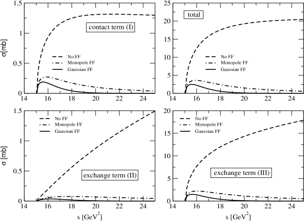
FIG. 2.: Upper right panel: total cross section for J/$\psi$ breakup by pion impact without formfactor (dashed line), with monopole type formfactor (dash-dotted line) and with Gaussian formfactor (solid line) as a function of the squared c.m. energy of initial - state mesons. The partial contributions from the diagrams I, II, and III of Fig. 1 shown in the other panels.

For the triangle diagrams, we use formfactors with a momentum dependence in the monopole form ($M$)

$$F_{3}^{M}({\bf q}^{2})=\frac{\Lambda^{2}}{\Lambda^{2}+{\bf q}^{2}}~{},$$ (59)

and in the Gaussian ($G$) form

$$F_{3}^{G}({\bf q}^{2})=\exp(-{{\bf q}^{2}/\Lambda^{2}})~{}.$$ (60)

At this point we have to add the comment that this choice, however, is obviously not supported by the underlying quark substructure diagrams that can provide a justification for the use of formfactors: While the triangle diagram is of third order in the wave functions so that the meson exchange diagrams are suppressed at large momentum transfer by six wave functions, the box diagram appears already at fourth order thus being less suppressed than suggested by the ansatz (57) of Ref. [10]. A proper analysis of the resulting discrepancy is beyond the scope of the present paper and has to be deferred to future work. For the cross section of the three diagrams including the effect of hadronic formfactors, we multiply the bare expressions with the formfactors given above. The results are depicted in Fig. 2. In the last section, we want to discuss the results and their possible implications for phenomenological applications.

FIG. 3.: Total J/$\psi$ breakup cross section with Gaussian formfactor ($\Lambda=0.9$ GeV - dot-dashed line, $\Lambda=0.8$ GeV - dot-dot-dashed line) compared to the nonrelativistic quark exchange model (Wong et al. [15] - solid line) and its parametrization by Burau et al. [8] (dashed line).

E Results and Discussion

The J/$\psi$ breakup cross section by $\pi$ and $\rho$ meson impact has been formulated within a chiral $U(4)$ Lagrangian approach. Numerical results have been obtained for the pion impact processes with the result that the D-meson exchange in the t-channel is the dominant subprocess contributing to the J/$\psi$ breakup. The use of formfactors at the meson-meson vertices is mandatory since otherwise the high-energy asymptotics of the processes with hadronic final states will be overestimated, see Fig. 2. From a comparison with results of a nonrelativistic potential model calculation, we can choose the shape of the formfactor to be Gaussian and fix the range $\Lambda=0.9$ GeV from the asymptotic high energy behaviour, see Fig. 3. Within our semi-quantitative discussion, we do not attempt a high accuracy description of the nonrelativistic result which accounts for another final state D-meson pair, see [12, 15].

Finally, we want to present an exploration of the influence of a variation of the final state D-meson masses on the effective J/$\psi$ breakup cross section. Our motivation for considering mesonic states to be off their mass-shell is their compositeness which can become apparent in a high-temperature (and density) environment at the deconfinement/chiral restoration transition, when these states change their character qualitatively being resonant quark- antiquark scattering states in the quark plasma rather than on-shell mesonic bound states.

The consequence of this Mott-transition from bound to resonant states for the J/$\psi$ breakup has been explored by Burau et al. [8, 7], see also these proceedings, using a fit formula for the D-mass dependence of the breakup cross section which shows a strong enhancement when the process becomes subthreshold ($M_{D}<M_{D}^{\rm vac}$). This behaviour is qualitatively approved within the present chiral U(4) Lagrangian + formfactor model although the subthreshold enhancement is more moderate, see Fig. 4. A more consistent description should include a quark model derivation of the formfactors for the meson-meson vertices and their possible medium dependence. Such an investigation is in progress.

FIG. 4.: Total J/$\psi$ breakup cross section in the chiral Lagrangian model with Gaussian formfactor ($\Lambda=0.9$ GeV - solid line) compared to the parametrization of the nonrelativistic quark exchange model [15] by Burau et al. [8] (dashed line). The four panels illustrate the differences between both models when the final state masses $M_{D_{1}}=M_{D_{2}}=M_{D}$ are varied.

Acknowledgement

V.I. and Yu.K. acknowledge support from the Deutsche Forschungsgemeinschaft under grant no. 436 RUS 17/102/00 and from the Ministery for Education, Science and Culture of Mecklenburg-Western Pommerania.

Mott Effect and Anomalous $J/\psi$ Suppression

Gerhard R.G. Burau^a, David B. Blaschke^a and Yuri L. Kalinovsky^b

^aFachbereich Physik, Universität Rostock, D-18051 Rostock, Germany
^bLaboratory of Information Technologies, JINR, 141980 Dubna, Russia

A Introduction

Recent results of the CERN NA50 collaboration on anomalous $J/\psi$ suppression [1] in ultrarelativistic Pb-Pb collisions at 158 AGeV have renewed the quest for an explanation of the processes which may cause the rather sudden drop of the $J/\psi$ production cross section for transverse energies above $E_{T}\sim 40$ GeV in this experiment. An effect like this was predicted as a signal for quark gluon plasma formation [2] due to screening of the $c\bar{c}$ interaction. Soon after that it became clear that for temperatures and densities just above the deconfinement transition the Mott effect for the $J/\psi$ does not occur and that a kinetic process is required to dissolve the $J/\psi$ [3] in a break-up process by impact of thermal photons [4], quarks [5], gluons [6] or mesons [7, 8].

In this paper, we suggest that at the chiral/deconfinement phase transition the charmonium break-up reaction cross sections are critically enhanced since the light and open-charm mesonic states of the dissociation processes become unbound (Mott effect) so that the reaction thresholds are effectively lowered. We present a model calculation for the particular process $J/\psi+\pi\to D+\bar{D}^{*}+h.c.$ in a hot gas of resonant (unbound but correlated) quark-antiquark states in order to demonstrate that the Mott dissociation of the final states (D-mesons) at the chiral phase transition leads to a threshold effect for the in-medium $J/\psi$ break-up cross section and thus the survival propability.

B In-medium modification of charmonium break-up cross sections

The inverse lifetime of a charmonium state in a hot and dense many-particle system is given by the imaginary part of its selfenergy

$$\tau^{-1}(p)=\Gamma(p)=\Sigma^{>}(p)-\Sigma^{<}(p)~{}.$$ (1)

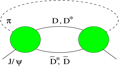
FIG. 1.: Diagrammatic representation of the complex selfenergy for the $J/\psi$ due to break-up in (off-shell) $D$, $\bar{D}^{*}$ pairs by impact of (off-shell) pions from a hot medium.

In the Born collision approximation for the dominant process in a hot gas of pion-like correlations, as shown in Fig. 1, we have [9]

$$\Sigma^{\stackrel{{\scriptstyle>}}{{<}}}(p)=\int\limits_{p^{\prime}}\int\limits_{p_{1}}\int\limits_{p_{2}}(2\pi)^{4}\delta_{p,p^{\prime};p_{1},p_{2}}\left|{\cal M}\right|^{2}G^{\stackrel{{\scriptstyle<}}{{>}}}_{\pi}(p^{\prime})~{}G^{\stackrel{{\scriptstyle>}}{{<}}}_{D_{1}}(p_{1})~{}G^{\stackrel{{\scriptstyle>}}{{<}}}_{D_{2}}(p_{2})~{},$$ (2)

where the thermal Green functions $G^{>}_{i}(p)=[1+f_{i}(p)]A_{i}(p)$ and $G^{<}_{i}(p)=f_{i}(p)A_{i}(p)$ are defined by the spectral function $A_{i}(p)$ and the distribution function $f_{i}(p)$ of the bosonic state $i$; with the notation $\delta_{p,p^{\prime};p_{1},p_{2}}=\delta(p+p^{\prime}-p_{1}-p_{2})$, $\int\limits_{p}=\int\frac{d^{4}p}{(2\pi)^{4}}$.

In the low density approximation for the final states ($f_{D_{i}}(p)\approx 0$), one can safely neglect $\Sigma^{<}(p)$ so that

$$\tau^{-1}(p)=\int\limits_{p^{\prime}}\int\limits_{p_{1}}\int\limits_{p_{2}}(2\pi)^{4}\delta_{p,p^{\prime};p_{1},p_{2}}\left|{\cal M}\right|^{2}f_{\pi}(p^{\prime})~{}A_{\pi}(p^{\prime})~{}A_{D_{1}}(p_{1})~{}A_{D_{2}}(p_{2}).$$ (3)

With the differential cross section

$$\frac{d\sigma}{dt}=\frac{1}{16\pi}\frac{\left|{\cal M}(s,t)\right|^{2}}{\lambda(s,M_{\psi}^{2},s^{\prime})}~{},$$ (4)

using $s=(p+p^{\prime})^{2}$, $t=(p-p_{1})^{2}$, $s^{\prime}=p^{\prime 2}$ and $\lambda(s,M_{\psi}^{2},s^{\prime})=[s-(M_{\psi}+\sqrt{s^{\prime}})^{2}][s-(M_{\psi}-\sqrt{s^{\prime}})^{2}]=4~{}v^{2}_{\rm rel}~{}[{\bf p}^{2}+M_{\psi}^{2}][{\bf p^{\prime}}^{2}+s^{\prime}]$ one can show that the $J/\psi$ relaxation time in a hot pion as well as pionic resonance gas is given by

$$\tau^{-1}(p)=\int\frac{d^{3}{\bf p^{\prime}}}{(2\pi)^{3}}\int ds^{\prime}f_{\pi}({\bf p^{\prime}},s^{\prime})~{}A_{\pi}(s^{\prime})v_{\rm rel}~{}\sigma^{*}(s)~{},$$ (5)

where depending on the properties of the medium the pion spectral function (as well as the D-meson spectral functions) describes either $q\bar{q}$ bound states or resonant (off-shell) correlations. The in-medium break-up cross section is given by

$$\sigma^{*}(s)=\int ds_{1}~{}ds_{2}~{}A_{D_{1}}(s_{1})~{}A_{D_{2}}(s_{2})~{}\sigma(s;s_{1},s_{2})~{}.$$ (6)

Note that there are two kinds of medium effects due to (i) the spectral functions of the final states and (ii) the explicit medium dependence of the matrix element ${\cal M}$. In the following model calculation we will use the approximation $\sigma(s;s_{1},s_{2})\approx\sigma^{\rm vac}(s;s_{1},s_{2})$ justified by the locality of the transition matrix ${\cal M}$ which makes it rather inert against medium influence.

C Model calculation

The quark exchange processes in meson-meson scattering can be calculated within the diagrammatic approach of Barnes and Swanson [10] which allows a generalization to finite temperatures in the thermodynamic Green function technique [11]. This technique has been applied to the calculation of $J/\psi$ break-up cross sections by pion impact in [8]. The approach has been extended to excited charmonia states and consideration of rho-meson impact recently [12]. The generic form of the resulting cross section (given a band of uncertainty) can be fit to the form

$$\sigma^{\rm vac}(s;M_{D_{1}}^{2},M_{D_{2}}^{2})=\sigma_{0}\ln(s/s_{0})\exp(-s/\lambda^{2})\quad,\quad s\geq s_{0}~{},$$ (7)

where $s_{0}=(M_{D_{1}}+M_{D_{2}})^{2}$ is the threshold for the process to occur, $\sigma_{0}=7.5\cdot 10^{9}$ mb and $\lambda=0.9$ GeV.

Recently, the charmonium dissociation processes have been calculated also in an effective Lagrangian approach [13, 14], but the freedom of choice for the formfactors of meson-meson vertices makes predictions uncertain. The development of a unifying approach on the basis of a relativistic confining quark model is in progress [15] and will remove this uncertainty by providing a derivation of the appropriate formfactors from the underlying quark substructure.

The major modification of the charmonium break-up process which we expect at finite temperatures in a hot medium of strongly correlated quark-antiquark states comes from the Mott effect for the light as well as the open-charm mesons. At finite temperatures when the chiral symmetry in the light quark sector is restored, the continuum threshold for light-heavy quark pairs drops below the mass of the D-mesons so that they are no longer bound states constrained to their mass shell, but become rather broad resonant correlations in the continuum. This Mott effect has been discussed within relativistic quark models [16] for the light meson sector but can also be generalized to the case of heavy mesons [17]. Applying a confining quark model [18] we have obtained the critical temperatures $T^{\rm Mott}_{D^{*}}=130$ MeV, $T^{\rm Mott}_{D}=140$ MeV and $T^{\rm Mott}_{\pi}=150$ MeV [15].

In order to study the implications of the pion and $D$-meson Mott effect for the charmonium break-up we adopt here a Breit-Wigner form for the spectral functions

$$A_{i}(s) = \frac{1}{\pi}\frac{\Gamma_{i}(T)~{}M_{i}(T)}{(s-M_{i}^{2}(T))^{2}+\Gamma_{i}^{2}(T)M_{i}^{2}(T)}~{},$$ (8)

which in the limit of vanishing width $\Gamma_{i}(T)\to 0$ goes over into the delta function $\delta(s-M_{i}^{2})$ for a bound state in the channel $i$. The width of the pions as well as the $D$-mesons shall be modeled by a microscopic approach. For our exploratory calculation, we adopt here

$$\Gamma_{\pi,D}(T)=c~{}(T-T^{\rm Mott}_{\pi,D})~{}\Theta(T-T^{\rm Mott}_{\pi,D})~{},$$ (9)

where the coefficient $c=2.67$ is assumed to be universal for the pions and $D$-mesons and it is obtained from a fit to the pion width above the pion Mott temperature, see [19]. For the meson masses we have $M_{\pi,D}(T)=M_{\pi,D}+0.75~{}\Gamma_{\pi,D}(T)$. The result for the in-medium $J/\psi$ break-up cross section (6) is shown in Fig. 2.

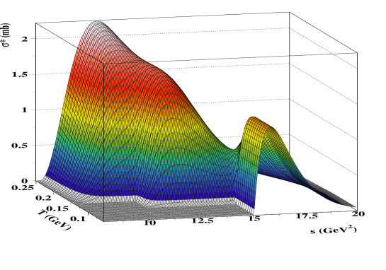
FIG. 2.: Energy- and temperature dependent in-medium $J/\psi$ break-up cross section for pion impact. Thresholds occur at the Mott temperatures for the open-charm mesons: $T^{\rm Mott}_{D^{*}}=130$ MeV, $T^{\rm Mott}_{D}=140$ MeV.

With $M_{D^{*}}=2.01$ GeV and $M_{\bar{D}}=1.87$ GeV follows for the threshold $s_{0}=15.05$ GeV². At a temperature $T=140$ MeV, where the D-meson can still be considered as a true bound state, the $D^{*}$-meson has already entered the continuum and is a resonance with a half width of about 80 MeV. Due to the Mott effect for the open-charm mesons (final states), the charmonium dissociation process become ”subthreshold” ones and their cross sections which are peaked at threshold rise and spread to lower onset with cms energy. This is expected to enhance strongly the rate for the charmonium dissociation processes in a hot resonance gas. To simplify matters we can assume a uniform Mott temperature for the D- and D^∗-meson amounting to $T_{\pi}^{\rm Mott}$. In this scenario we find of course only one threshold in the temperature behavior of the in-medium $J/\psi$ break-up cross section (6).

D $J/\psi$ dissociation in a hot “pion” gas

We calculate the inverse relaxation time for a $J/\psi$ at rest in a hot gas of pions (below $T_{\pi}^{\rm Mott}$) and pion-like correlations (above $T_{\pi}^{\rm Mott}$) by specifying Eq. (5) for this simplified case

$$\tau^{-1}(T) = \int\frac{d^{3}{\bf p^{\prime}}}{(2\pi)^{3}}\int ds_{\pi}A_{\pi}(s_{\pi})f_{\pi}({\bf p^{\prime}},s_{\pi};T)\frac{|{\bf p^{\prime}}|}{E_{\pi}({\bf p^{\prime}},s_{\pi})}\sigma^{*}(s)$$ (10)

$$= <\sigma^{*}v_{\rm rel}>n_{\pi}(T)~{},$$ (12)

with the dispersion relation $E_{\pi}({\bf p^{\prime}},s_{\pi})=\sqrt{{\bf p^{\prime}}^{2}+s_{\pi}}$, the thermal Bose distribution function $f_{\pi}({\bf p^{\prime}},s_{\pi};T)=3\left\{\exp[E_{\pi}({\bf p^{\prime}},s_{\pi})/T]-1\right\}^{-1}$ and the particle density $n_{\pi}(T)$ for the “pions”. The cms energy of the “pion” impact on a $J/\psi$ at rest is $s({\bf p^{\prime}};s_{\pi})=s_{\pi}+M_{\psi}^{2}+2M_{\psi}E_{\pi}({\bf p^{\prime}},s_{\pi})$.

The result for the temperature dependence of the thermal averaged $J/\psi$ break-up cross section $<\sigma^{*}v_{\rm rel}>$ is shown in Fig. 3. This quantity has to be compared to the nuclear absorption cross section for the $J/\psi$ of about 3 mb which has been extracted from charmonium suppression data in p-A collisions [20].

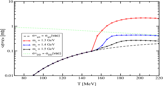
FIG. 3.: Temperature dependence of the thermal averaged in-medium $J/\psi$ break-up cross section for different charm quark masses with off-shell effects for $\pi$, $D$ and $D^{*}$ above $T^{Mott}=T_{c}=150$ MeV. The dotted line shows the thermal averaged cross section for the back process ($DD^{*}$ annihilation) without Mott effect.

It is remarkable that it is practically negligible below the Mott temperature $T^{\rm Mott}=150$ MeV for the open-charm mesons but comparable to the nuclear absorption cross section above the chiral/deconfinement temperature of $T_{\rm crit}\approx 150$ MeV. It is obvious that the transition from D-meson bound states to unbound light-heavy quark correlations is responsible for the strong increase by one to two orders of magnitude. Note that in this calculation the Mott effect for the pion (initial state) above $T^{\rm Mott}_{\pi}$ has been also included, but does not alter the result obtained previously [21] in a calculation neglecting this effect.

Therefore we expect the in-medium enhanced charmonium dissociation process to be sufficiently effective to destroy the charmonium state on its way through the hot fireball of the heavy-ion collision and to provide an explanation of the observed anomalous $J/\psi$ suppression phenomenon [1]. A detailed comparison with the recent data from the NA50 collaboration requires a model for the heavy-ion collision. The effective in-medium break-up cross section for the $J/\psi$ derived in this work provides an input for all calculations which use this quantity, e.g. Glauber-type models [21, 22, 23, 24, 25, 26], more detailed calculations based on a parton cascade model [27] or molecular dynamics [28].

E Summary and Outlook

In this contribution we have presented an approach to charmonium break-up in a hot and dense medium which is applicable in the vicinity of the chiral/deconfinement phase transition where mesonic bound states get dissolved in a Mott-type transition and should be described as resonant correlations in the quark plasma. This description can be achieved using the concept of the spectral function which can be obtained from relativistic quark models in a systematic way. The result of an exploratory calculation employing a temperature-dependent Breit-Wigner spectral function for light and open-charm mesons presented in this work has demonstrated that heavy-flavor dissociation processes are critically enhanced at the QCD phase transition and could represent the physical mechanism behind the phenomenon of anomalous $J/\psi$ suppression.

In subsequent work we will relax systematically approximations which have been made in the present paper and improve inputs which have been used. In particular, we will investigate the off-shell behaviour of the charmonium break-up cross section in the vacuum (7) and calculate the spectral functions (8) at finite temperature within a relativistic quark model. Dyson-Schwinger equations provide a nonperturbative, field-theoretical approach which has recently been applied also to heavy-meson observables [29] and have proven successful for finite-temperature generalization [30, 31]. Further intermediate open-charm states can be considered; the states in the dense environment should include rho mesons and nucleons besides of the pions which all can be treated as off-shell quark correlations at the QCD phase transition.

In future experiments at LHC the charm distribution in the created fireball may be not negligible so that the approximation $f_{D_{i}}(p)\approx 0$ has to be relaxed. In this case, one has to include the gain process ($D\bar{D}$ annihilation) encoded in the $\Sigma^{<}$ function. In comparision to previous investigations [32, 33] the present quantum kinetic treatment contains Bose enhancement factors in the $G^{>}_{i}$ functions which modify the charm equilibration process.

Acknowledgements

This work has been supported by the Heisenberg-Landau program for scientific collaborations between Germany and the JINR Dubna and by the DFG Graduiertenkolleg “Stark korrelierte Vielteilchensysteme” at the University of Rostock. We thank T. Barnes, P. Braun-Munzinger, J. Hüfner, M.A. Ivanov, C.D. Roberts, G. Röpke, S.M. Schmidt and P.C. Tandy for their discussions and stimulating interest in our work.

Few-Body Correlations in Fermi Systems

M. Beyer

FB Physik, University of Rostock, 18051 Rostock, Germany

Interacting quantum systems with strong or long-range interactions exhibit quite a rich phase structure. Cluster formation and superconductivity are examples. These phenomena are also expected in the astrophysical context, e.g., during the formation or in the structure of neutron stars. To describe these phenomena a proper treatment has to go beyond the simple picture of noninteracting quasiparticles. An appealing formalism for a systematic approach is provided by the framework of Dyson equations. Within an equal (imaginary) time formalism Dyson equations can be derived for an arbitrary large cluster embedded in a medium [1]. For practical use and the sake of simplicity the medium is treated as uncorrelated to derive the respective $n$-body cluster Green functions. Further, we neglect “backward” propagating particles, so the Fock spaces for different number of particles $n$ are disconnected. This way it is possible to derive effective in-medium $n$-body equations that can be solved rigorously with few-body techniques [2, 3, 4, 5, 6, 7, 8, 9, 10, 11, 12, 13].

These resulting two-, three-, and four-body equations elaborated here include the dominant medium effects in a systematic way. These are the self energy corrections for masses and the Pauli blocking that in turn leads to a change of binding energies, viz. change of the masses of clusters, and change of reaction rates. Further, within this approach the critical temperatures for condensation (of bosons containing two or four particles) are calculated.

Defining $H_{0}=\sum_{i=1}^{n}\varepsilon_{i}$ with the quasi-particle self energy

$$\varepsilon_{1}=k^{2}_{1}/2m_{1}+\sum_{2}V_{2}(12,\widetilde{12})f_{2}$$ (1)

and the Fermi function $f_{1}\equiv f(\varepsilon_{1})=1/(e^{\beta(\varepsilon_{1}-\mu)}+1),$ the $n$-particle cluster resolvent $G_{0}$ is

$$G_{0}(z)=(z-H_{0})^{-1}\;{N}\equiv R_{0}(z)\;{N}.$$ (2)

Here $G_{0}$, $H_{0}$, and $N$ are matrices in $n$ particle space and $z$ denotes the Matsubara frequency [14]. The Pauli-blocking factors for $n$-particles are

$$N=\bar{f}_{1}\bar{f}_{2}\dots\bar{f}_{n}\pm f_{1}f_{2}\dots f_{n},\qquad\bar{f}=1-f$$ (3)

Note: $NR_{0}=R_{0}N$. Defining the effective potential $V\equiv\sum_{\mathrm{pairs}\;\alpha}{N_{2}^{\alpha}}V_{2}^{\alpha}$ the full and the channel resolvents are

$$G(z) = (z-H_{0}-V)^{-1}{N}\equiv R(z){N},$$ (4)

$$G_{\alpha}(z) = (z-H_{0}-{N_{2}^{\alpha}}V_{2}^{\alpha})^{-1}{N}\equiv R_{\alpha}(z){N},$$ (5)

Note that $V^{\dagger}\neq V$ and $R(z)N\neq NR(z)$. For the scattering problem it is convenient to define the in-medium AGS operator $U_{\beta\alpha}(z)$

$$R(z)=\delta_{\alpha\beta}R_{\beta}(z)+R_{\beta}(z){U_{\beta\alpha}(z)}R_{\alpha}(z)$$ (6)

that after some algebra leads to the in-medium AGS equation

$$U_{\beta\alpha}(z)=\bar{\delta}_{\beta\alpha}R_{0}(z)^{-1}+\sum_{\gamma}\bar{\delta}_{\beta\gamma}N_{2}^{\gamma}T_{2}^{\gamma}(z)R_{0}(z)U_{\gamma\alpha}(z),$$ (7)

where $\bar{\delta}_{\beta\alpha}=1-\delta_{\beta\alpha}$. The square of this $t$-operator is directly linked to the differential cross section for the scattering process $\alpha\rightarrow\beta$. The driving kernel consists of the two-body $t$-matrix derived in the same formalism, however given earlier and known as Feynman-Galitskii equation[14]

$$T_{2}^{\gamma}(z) = V_{2}^{\gamma}+V_{2}^{\gamma}{N^{\gamma}_{2}}R_{0}(z)T_{2}^{\gamma}(z).$$ (8)

A numerical solution using a coupled Yamaguchi potential has been given in Ref. [2]. For a temperature $T=10$ MeV and the three-body system at rest in the medium results a given in Fig.1 For the bound state problem it is convenient to introduce form factors

$$|F_{\beta}\rangle=\sum_{\gamma}\bar{\delta}_{\beta\gamma}{N_{2}^{\gamma}}V_{2}^{\gamma}|\psi_{B_{3}}\rangle.$$ (9)

Since the potential is nonsymmetric right and left eigenvectors are different, although the bound state energies are the same,

$$|F_{\alpha}\rangle = \sum_{\beta}\bar{\delta}_{\alpha\beta}{N_{2}^{\beta}}T_{2}^{\beta}(B_{3})R_{0}(B_{3})|F_{\beta}\rangle,$$ (10)

$$|\tilde{F}_{\alpha}\rangle = \sum_{\beta}\bar{\delta}_{\alpha\beta}T_{2}^{\beta}(B_{3}){N_{2}^{\beta}}R_{0}(B_{3})|\tilde{F}_{\beta}\rangle.$$ (11)

FIG. 1.: Break-up cross section for different densities of nuclear matter for temperature $T=10$ MeV

The binding energy depends on $\mu,\;T,\;P_{\mathrm{c}.m.}$. Results for $P_{\mathrm{c}.m.}=0$ are given in Fig.2 for different potentials and temperatures. Note that the dependence on density is rather similar for two different potentials studied, although the binding energies for the isolated triton differs by 10% the Mott density is practically at the same place once the binding energies are renormalized to each other. For helium the Mott density is smaller due to the Coulomb force, however for asymmetric nuclear matter, e.g. $N_{p}/N_{n}\simeq 0.72$ (for the ¹²⁹Xe$+~{}^{119}$Sn reaction) this effect is compensated [15]. The dependence of the Mott effect on the momentum is given in Ref. [5].

We now turn to the four-body problem in matter. In addition to having different channels as for the three body system now the channels appear in different partitions that makes the four-body problem even more involved. The partitions of the four-body clusters are denoted by $\rho,\tau,\sigma,\dots$, e.g., $\rho=(123)(4),(234)(1),\dots$ for $3+1$-type partitions, or $\rho=(12)(43),(23)(41),\dots$ for $2+2$-type partitions. The two-body sub-channels are denoted by pair indices $\alpha,\beta,\gamma,\dots$, e.g. pairs $(12)$, $(24)$,…The two- and three-body $t$-matrices have to be defined with respect to the partitions that leads to additional indices. The four-body in-medium homogeneous AGS equation are defined for the form factors

FIG. 2.: Triton binding energy as a function of nuclear matter density. Dashed-dot-dot $T=10$ MeV, other $T=20$ MeV.

$$|{\cal F}_{\beta}^{\sigma}\rangle=\sum_{\tau}\bar{\delta}_{\sigma\tau}\sum_{\alpha}\bar{\delta}^{\tau}_{\beta\alpha}R_{0}^{-1}(B_{4})|\psi_{\alpha}\rangle,$$ (12)

where $\bar{\delta}^{\tau}_{\beta\alpha}=\bar{\delta}_{\beta\alpha}$, if $\beta,\alpha\subset\tau$ and $\bar{\delta}^{\rho}_{\beta\alpha}=0$ otherwise and $|\psi_{\alpha}\rangle$ is the $\alpha$- particle wave function. They read [8]

$$|{\cal F}^{\sigma}_{\beta}\rangle=\sum_{\tau\gamma}\bar{\delta}_{\sigma\tau}U^{\tau}_{\beta\gamma}(B_{4})R_{0}(B_{4}){N_{2}^{\gamma}}T_{2}^{\gamma}(B_{4})R_{0}(B_{4})|{\cal F}^{\tau}_{\gamma}\rangle,$$ (13)

where $\alpha\subset\sigma,\gamma\subset\tau$. A numerical solution of this equation is rather complex. In order to reduce computational time we introduce a energy dependent pole expansion (EDPE) that has been proven useful in many application involving the $\alpha$-particle and is accurate enough for the present purpose. However, we have to generalize the original version of the EDPE because of different right and left eigenvectors. Details will be omitted here, see [8]

In the two-body sub-system the EDPE reads

$$T_{\gamma}(z) \simeq \sum_{n}|\tilde{\Gamma}_{\gamma n}(z)\rangle t_{\gamma n}(z)\langle\Gamma_{\gamma n}(z)|\simeq\sum_{n}|\tilde{g}_{\gamma n}\rangle t_{\gamma n}(z)\langle g_{\gamma n}|$$ (14)

$$= \sum_{n}{N_{2}^{\gamma}}|g_{\gamma n}\rangle t_{\gamma n}(z)\langle g_{\gamma n}|.$$ (15)

where we have chosen a Yamaguchi ansatz for the form factors for simplicity. Inserting this ansatz into the Feynman-Galitskii equation determines the propagator $t_{\gamma n}(z)$. In the three-body sub-system the EDPE expansion reads

$$\langle g_{\beta m}(z)|R_{0}(z)U^{\tau}_{\beta\gamma}(z)R_{0}(z)|\tilde{g}_{\gamma n}(z)\rangle\simeq\sum_{t,\mu\nu}|\tilde{\Gamma}^{\tau t,\mu}_{\beta m}(z)\rangle t^{\tau t}_{\mu\nu}(z)\langle\Gamma^{\tau t,\nu}_{\gamma n}(z)|.$$ (16)

with the three-body EDPE functions

$$|\tilde{\Gamma}^{\tau t,\mu}_{\beta m}(z)\rangle=\langle g_{\alpha n}|R_{0}(z)|\tilde{g}_{\beta m}\rangle t_{\beta m}(B_{3})|\tilde{\Gamma}^{\tau t,\mu}_{\beta m}\rangle,$$ (17)

that we get from solving the proper Sturmian equations

$$\eta_{t,\mu}|\tilde{\Gamma}^{\tau t,\mu}_{\alpha n}\rangle = \sum_{\beta m}\langle g_{\alpha n}|R_{0}(B_{3})|\tilde{g}_{\beta m}\rangle t_{\beta m}(B_{3})|\tilde{\Gamma}^{\tau t,\mu}_{\beta m}\rangle$$ (18)

$$\eta_{t,\mu}|\Gamma^{\tau t,\mu}_{\alpha n}\rangle = \sum_{\beta m}\langle\tilde{g}_{\alpha n}|R_{0}(B_{3})|g_{\beta m}\rangle t_{\beta m}(B_{3})|\Gamma^{\tau t,\mu}_{\beta m}\rangle$$ (19)

Inserting everything into the homogeneous AGS equations allows us to redefine the form factors that are now operators in the coordinates of the $2+2$ or $3+1$ system, respectively

$$|\Gamma^{\sigma s}_{\mu}\rangle=\sum_{\beta m}\langle\Gamma^{\sigma s}_{\beta m,\nu}(B_{4})|t_{\beta m}(B_{4})\langle g_{\beta m}(B_{4})|R_{0}(B_{4})|{\cal F}^{\sigma}_{\beta}\rangle$$ (20)

and therefore the final homogeneous equation

$$|\Gamma^{\sigma s}_{\mu}\rangle=\sum_{\tau t}\sum_{\nu\kappa}\sum_{\gamma n}\bar{\delta}_{\sigma\tau}\langle\Gamma^{\sigma s,\nu}_{\gamma n}(B_{4})|t_{\gamma n}(B_{4})|\tilde{\Gamma}^{\sigma s,\mu}_{\gamma n}(B_{4})\rangle\;t^{\tau t}_{\mu\kappa}(B_{4})\;|\Gamma^{\tau t}_{\kappa}\rangle,$$ (21)

is an effective one-body equation with and effective potential ${\cal V}$ and an effective resolvent ${\cal G}_{0}$:

$${\cal V}^{\sigma s,\tau t}_{\mu\nu}(z) = \sum_{\gamma n}\bar{\delta}_{\sigma\tau}\langle\Gamma^{\sigma s,\mu}_{\gamma n}(z)|t_{\gamma n}(z)|\tilde{\Gamma}^{\sigma s,\nu}_{\gamma n}(z)\rangle,$$ (22)

$${\cal G}^{\sigma s,\tau t}_{\mu\nu,0}(z) = t^{\tau t}_{\mu\nu}(z).$$ (23)

FIG. 3.: Energy dependence of the binding energy of the $\alpha$-particle

The binding energies of the two-, three-, and four-body systems are shown in Fig.3 for a temperature of $T=10$ MeV and a c.m. momentum of the respective cluster of $P_{\mathrm{c}.m.}=0$. The $B=0$ line reflects the respective continuum. Investigating the zeros of the two-body Joost function the quasi deuteron survives as an anti-bound state (not resonance) with increasing densities, viz. for energies above the continuum[16]. The fate of the triton and of the $\alpha$ particle for $B>0$ still needs to investigated as well as a possible appearance of Efimov states related to $B\rightarrow 0$ of the sub-system. Since the Efimov states are ’excited’ states, e.g. for the three-body system close to the $2+1$ threshold, their blocking may be smaller since the wave functions contain higher momentum components. Note that the slope of the binding energies as a function of densities for the larger clusters is also larger. This is a clear indication that the masses of the clusters change with increasing density. The Mott density of the $\alpha$ particle appears at

$$B_{4}(n_{\mathrm{M}ott}=0.19{\mathrm{f}m}^{-3},T=10\mbox{ MeV},P_{\mathrm{c}.m.}=0)=0$$

FIG. 4.: Temperature vs. effective chemical potential ($\mu^{*}=\mu-\Sigma(0)$), $\Sigma(0)$ Hartree-Fock shift of the single particle energy at zero momentum. Lines show the critical temperature for pairing (solid) and quartetting. The dashed line shows a result given in [17], the diamonds show the solution of the AGS equation given in (21)

For comparison a perturbative result using Gaussian functions fitted to the charge radius of the $\alpha$-particle is also given.

Finally, I address the question of a possible four-particle condensate or quartetting [17]. The condition is $B_{4}(n,T_{c},P_{\mathrm{c}.m.}=0)=4\mu$. From Fig.3 we argue that $\alpha$ condensation is likely, i.e.

$$T_{c}^{\alpha}>T_{c}^{\mathrm{N}N},$$

where the critical temperature for $\alpha$ condensation turns out to be higher than for the pairing. However, for $\mu>0$ the situation seems not so clear, since the four-body AGS equation (21) develops poles related to zeros in $4\mu-H_{0}$. Unlike the two-body case were these poles disappear because the numerator becomes as well zero at $2\mu$ and $T_{c}$ (viz. $1-f_{1}-f_{2}\rightarrow 0$). A vanishing numerator is not obvious for the four-body case because there are more channels involved. It remains to be clarified, if the rapid fall of the critical temperature found in Ref. [17] using variational treatment with square-integrable functions remains, if one uses an exact treatment of the four-body problem. This is currently investigated.

Acknowledgment I am very grateful to S. Mattiello, C. Kuhrts, G. Röpke, P. Schuck, S.A. Sofianos, and W. Schadow, who have contributed in certain stages to some results presented here, and to T. Frederico for lively discussions. I gratefully acknowledge the warm and pleasant atmosphere at the Department of Physics during stays at UNISA, Pretoria. Work supported by Deutsche Forschungsgemeinschaft and University of South Africa.

Statistical Multifragmentation in Thermodynamical Limit: An Exact Solution for Phase Transitions

K.A. Bugaev^1,2, M.I. Gorenstein^1,2, I.N. Mishustin^1,3,4 and

W. Greiner¹

¹ Institut für Theoretische Physik, Universität Frankfurt, Germany
² Bogolyubov Institute for Theoretical Physics, Kyiv, Ukraine
³ Kurchatov Institute, Russian Research Center, Moscow, Russia
⁴ Niels Bohr Institute, University of Copenhagen, Denmark

Key words: Nuclear matter, 1-st order liquid-gas phase

transition, mixed phase thermodynamics

PACS: 21.65.+f, 24.10. Pa, 25.70. Pq

Nuclear multifragmentation is one of the most interesting and widely discussed phenomena in intermediate energy nuclear reactions. The statistical multifragmentation model (SMM) (see [1, 2] and references therein) was recently applied to study the liquid-gas phase transition in nuclear matter [3, 4, 5, 6]. Numerical calculations within the canonical ensemble exhibited many intriguing peculiarities of the finite multifragment systems. However, the investigation of the system’s behavior in the thermodynamic limit was still missing. Therefore, there was no rigorous proof of the phase transition existence, and the phase diagram structure of the SMM remained unclear. Previous numerical studies for the finite nuclear systems (the canonical and microcanonical ensembles) led to unjustified (and sometimes wrong) statements concerning the nuclear liquid-gas phase transition in the thermodynamic limit. In our recent paper [7] an exact analytical solution of the SMM was found within the grand canonical ensemble which naturally allowed to study the thermodynamic limit. The self-consistent treatment of the excluded volume effects was an important part of this study. In this letter we investigate the peculiar thermodynamic properties near the boundary between the mixed phase and the pure gaseous phase. New results for the caloric curve and the specific heat are presented and a physical picture of the nuclear liquid-gas phase transition in SMM is clarified. This physical picture differs from the one advocated in the previous numerical studies.

In the SMM the states of the system are specified by the multiplicity sets $\{n_{k}\}$ ($n_{k}=0,1,2,...$) of $k$-nucleon fragments. The partition function of a single fragment with $k$ nucleons is [1]: $\omega_{k}=V\left(mTk/2\pi\right)^{3/2}z_{k}~{}$, where $k=1,2,...,A$ ($A$ is the total number of nucleons in the system). $V$ and $T$ are, respectively, the volume and the temperature of the system, $m$ is the nucleon mass. The first two factors in $\omega_{k}$ originate from the non-relativistic thermal motion and the last factor, $z_{k}$, represents the intrinsic partition function of the $k$-fragment. For $k=1$ (nucleon) we take $z_{1}=4$ (4 internal spin-isospin states) and for fragments with $k>1$ we use the expression motivated by the liquid drop model (see details in Ref. [1]): $z_{k}=\exp(-f_{k}/T),$ with the fragment free energy

$$f_{k}~{}=~{}-[W_{\rm o}~{}+~{}T^{2}/\epsilon_{\rm o}~{}]k~{}+~{}\sigma(T)~{}k^{2/3}~{}+~{}\tau~{}T\ln k~{}.$$ (24)

Here $W_{\rm o}=16$ MeV is the bulk binding energy per nucleon, $T^{2}/\epsilon_{\rm o}$ is the contribution of the excited states taken in the Fermi-gas approximation ($\epsilon_{\rm o}=16$ MeV) and $\sigma(T)$ is the temperature dependent surface tension which is parameterized in the following form:

$$\sigma(T)=\sigma_{\rm o}[(T_{c}^{2}~{}-~{}T^{2})/(T_{c}^{2}~{}+~{}T^{2})]^{5/4},$$ (25)

with $\sigma_{\rm o}=18$ MeV and $T_{c}=18$ MeV ($\sigma=0$ at $T\geq T_{c}$). The last Fisher’s term in Eq. (24) with dimensionless parameter $\tau$ is introduced for generality. The canonical partition function (CPF) of the ensemble of nuclear fragments has the following form:

$$Z^{id}_{A}(V,T)~{}=~{}\sum_{\{n_{k}\}}~{}\prod_{k=1}^{A}~{}\frac{\omega_{k}^{n_{k}}}{n_{k}!}~{}\delta(A-\sum_{k}kn_{k})~{}.$$ (26)

The model defined by Eqs.(24,26) with $\tau=0$ was studied numerically in Refs. [3, 4, 5, 6]. This is a simplified version of the SMM since the symmetry-energy and Coulomb contributions are neglected. However, its investigation appears to be very important for understanding the physics of multifragmentation.

In Eq. (26) the nuclear fragments are treated as point-like objects. However, these fragments have non-zero proper volumes and they should not overlap in the coordinate space. In the Van der Waals excluded volume approximation this is achieved by replacing the total volume $V$ in Eq. (26) by the free (available) volume $V_{f}\equiv V-b\sum_{k}kn_{k}$, where $b=1/\rho_{{\rm o}}$ ($\rho_{{\rm o}}=0.16$ fm^-3 is the normal nuclear density). Therefore, the corrected CPF becomes: $Z_{A}(V,T)=Z^{id}_{A}(V-bA,T)$.

The calculation of $Z_{A}(V,T)$ is difficult because of the constraint $\sum_{k}kn_{k}=A$. This difficulty can be partly avoided by calculating the grand canonical partition function:

$${\cal Z}(V,T,\mu)~{}\equiv~{}\sum_{A=0}^{\infty}\exp\left(\mu A/T\right)~{}Z_{A}(V,T)~{}\Theta(V-bA)~{},$$ (27)

where the chemical potential $\mu$ is introduced. The calculation of ${\cal Z}$ is still rather difficult. The summation over the sets $\{n_{k}\}$ in $Z_{A}$ cannot be performed analytically because of the additional $A$-dependence in the free volume $V_{f}$ and the restriction $V_{f}>0$. The problem can be solved by introducing the so-called isobaric partition function (IPF) which is calculated in a straightforward way (see details in Refs. [7, 8, 9, 10]):

$$\hat{\cal Z}(s,T,\mu)~{}\equiv~{}\int_{0}^{\infty}dV~{}\exp(-sV)~{}{\cal Z}(V,T,\mu)~{}=~{}\frac{1}{s~{}-~{}{\cal F}(s,T,\mu)}~{},$$ (28)

where

$${\cal F}(s,T,\mu) = \left(\frac{mT}{2\pi}\right)^{3/2}\left[z_{1}\exp\left(\frac{\mu-sbT}{T}\right)\right.$$ (29)

$$+ \sum_{k=2}^{\infty}\left.k^{3/2-\tau}\exp\left(\frac{(\nu-sbT)k-\sigma k^{2/3}}{T}\right)\right]\,\,,$$ (30)

with $\nu\equiv\mu+W_{\rm o}+T^{2}/\epsilon_{\rm o}$. In the thermodynamic limit $V\rightarrow\infty$ the pressure of the system is defined by the farthest-right singularity, $s^{*}(T,\mu)$, of the IPF $\hat{\cal Z}(s,T,\mu)$

$$p(T,\mu)~{}\equiv~{}T~{}\lim_{V\rightarrow\infty}\frac{\ln~{}{\cal Z}(V,T,\mu)}{V}~{}=~{}T~{}s^{*}(T,\mu)~{}.$$ (31)

The study of the system’s behavior in the thermodynamic limit is therefore reduced to the investigation of the singularities of $\hat{\cal Z}$.

The IPF (28) has two types of singularities: 1) the simple pole singularity defined by the following equation $s_{g}(T,\mu)={\cal F}(s_{g},T,\mu)~{}$; 2) the singularity of the function ${\cal F}$ itself at the point $s_{l}(T,\mu)=\nu/Tb$ where the coefficient in linear over $k$ terms of the exponent in Eq. (30) is equal to zero.

The simple pole singularity corresponds to the gaseous phase where pressure $p_{g}\equiv Ts_{g}$ is determined by the following transcendental equation: $p_{g}(T,\mu)=T{\cal F}(p_{g}/T,T,\mu)$. The singularity $s_{l}(T,\mu)$ of the function ${\cal F}$ defines the liquid pressure: $p_{l}(T,\mu)\equiv Ts_{l}(T,\mu)={\nu}/{b}.$ Here the liquid is represented by an infinite fragment (condensate) with $k=\infty$.

In the region of the $(T,\mu)$-plane where $\nu<bp_{g}(T,\mu)$ the gaseous phase is realized ($p_{g}>p_{l}$), while the liquid phase dominates at $\nu>bp_{g}(T,\mu)$. The liquid-gas phase transition occurs when the two singularities coincide, i.e. $s_{g}(T,\mu)=s_{l}(T,\mu)$. As ${\cal F}$ in Eq. (30) is a monotonously decreasing function of $s$ the necessary condition for the phase transition is that the function ${\cal F}$ is finite in its singular point $s_{l}$. At $\tau=0$ this condition requires $\sigma(T)>0$ and, therefore, $T<T_{c}$. Otherwise, ${\cal F}(s_{l},T,\mu)=\infty$ and the system is always in the gaseous phase as $s_{g}>s_{l}$. As one can see from Eq.(30) the convergence properties of ${\cal F}(s,T,\mu)$ depend significantly on the Fisher’s exponent $\tau$ in the vicinity of the critical point where the surface term vanishes. In what follows we mainly concentrate on the case $\tau=0$. Other possibilities which appear at $\tau>0$ are discussed shortly. Their detail study can be found in Ref. [7]. Here we only note that Eqs. (28, 30) represent an exact solution of the Fisher’s droplet model [11] where additionally the effects of excluded volume are incorporated.

The baryonic density $\rho$ in the liquid and gaseous phases is given by the following formulae, respectively:

$$\rho_{l}\equiv\left(\partial p_{l}/\partial\mu\right)_{T}=1/b~{},~{}~{}~{}~{}\rho_{g}\equiv\left(\partial p_{g}/\partial\mu\right)_{T}=\rho_{id}/(1+b\rho_{id})~{},$$ (32)

where the function $\rho_{id}$ is the density of point-like nuclear fragments with shifted, $\mu\rightarrow\mu-bp_{g}$, chemical potential:

$$\rho_{id}(T,\mu) = \left(\frac{mT}{2\pi}\right)^{3/2}\left[z_{1}\exp\left(\frac{\mu-bp_{g}}{T}\right)\right.$$ (33)

$$+ \left.\sum_{k=2}^{\infty}k^{5/2}\exp\left(\frac{(\nu-bp_{g})k-\sigma k^{2/3}}{T}\right)\right]~{}.$$ (34)

At $T<T_{c}$ the system undergoes a 1-st order phase transition across the line $\mu^{*}=\mu^{*}(T)$ defined by the condition of coinciding singularities: $s_{l}=s_{g},$ i.e., $p_{l}=p_{g}$. The phase transition line $\mu^{*}(T)$ in the $(T,\mu)$-plane corresponds to the mixed liquid and gas states. This line is transformed into the finite mixed-phase region in the $(T,\rho)$-plane shown in Fig. 1. The baryonic density in the mixed phase is a superposition of the liquid and gas baryonic densities: $\rho=\lambda\rho_{l}+(1-\lambda)\rho_{g}~{},$ where $\lambda$ ($0<\lambda<1$) is the fraction of the system’s volume occupied by the liquid inside the mixed phase. Similar linear combinations are also valid for the entropy density $s$ and the energy density $\varepsilon$ with $(i=l,g)$ $s_{i}=\left(\partial p_{i}/\partial T\right)_{\mu}$ , $\varepsilon_{i}=T\left(\partial p_{i}/\partial T\right)_{\mu}+\mu\left(\partial p_{i}/\partial\mu\right)_{T}-p_{i}$.

Inside the mixed phase at constant density $\rho$ the parameter $\lambda$ has a specific temperature dependence shown in Fig. 2: from an approximately constant value $\rho/\rho_{\rm{o}}$ at small $T$ the function $\lambda(T)$ drops to zero in a narrow vicinity of the boundary separating the mixed phase and the pure gaseous phase. This corresponds to a fast change of the configurations from the state which is dominated by one infinite liquid fragment to the gaseous multifragment configurations. It happens inside the mixed phase without discontinuities in the thermodynamical functions.

An abrupt decrease of $\lambda(T)$ near this boundary causes a strong increase of the energy density as a function of temperature. This is evident from Fig. 3 which shows the caloric curves at different baryonic densities. One can clearly see a leveling of temperature at energies per nucleon between 10 and 20 MeV. As a consequence this leads to a sharp peak in the specific heat per nucleon at constant density, $c_{\rho}(T)\equiv(\partial\varepsilon/\partial T)_{\rho}/\rho~{}$, presented in Fig. 4. A finite discontinuity of $c_{\rho}(T)$ arises at the boundary between the mixed phase and the gaseous phase. This finite discontinuity is caused by the fact that $\lambda(T)=0$, but $(\partial\lambda/\partial T)_{\rho}\neq 0$ at this boundary (see Fig. 2).

The negative values of the specific heat shown in Fig. 4 appear due to the parameterization of the surface tension (25): its second derivative with respect to temperature generates a negative contribution in the vicinity of $T_{c}$ for all densities. This feature of the model is unphysical and it has to be modified.

It should be emphasized that the energy density is continuous at the boundary of the mixed phase and the gaseous phase, hence the sharpness of the peak in $c_{\rho}$ is entirely due to the strong temperature dependence of $\lambda(T)$ near this boundary. Moreover, at any $\rho<\rho_{\rm o}$ the maximum value of $c_{\rho}$ remains finite and the peak width in $c_{\rho}(T)$ is nonzero in the thermodynamic limit considered in our study. This is in contradiction with the expectation of Refs. [4, 5] that an infinite peak of zero width will appear in $c_{\rho}(T)$ in this limit. Also a comment about the so-called “boiling point” is appropriate here. This is a discontinuity in the energy density $\varepsilon(T)$ or, equivalently, a plateau in the temperature as a function of the excitation energy. Our analysis shows that this type of behavior indeed happens at constant pressure, but not at constant density! This is similar to the usual picture of a liquid-gas phase transition. In Refs. [4, 5] a rapid increase of the energy density as a function of temperature at fixed $\rho$ near the boundary of the mixed and gaseous phases (see Fig. 3) was misinterpreted as a manifestation of the “boiling point”.

The results presented in Figs. 1-4 are obtained for $\tau=0$. New possibilities appear at non-zero values of the parameter $\tau$. At $0<\tau\leq 5/2$ the qualitative picture remains the same as discussed above, although there are some quantitative changes. For $\tau>5/2$ the condition ${\cal F}(s,T,\mu)<\infty$ is also satisfied in the singularity point $s_{l}(T,\mu)$ for all $T>T_{c}$ where $\sigma(T)=0$. Therefore, the liquid-gas phase transition extends now to all temperatures. Its properties are, however, different for $\tau>7/2$ and for $\tau<7/2$ (see Fig. 5). If $\tau>7/2$ the gas density is always lower than $1/b$ as $\rho_{id}$ is finite. Therefore, the liquid-gas transition at $T>T_{c}$ remains the 1-st order phase transition with discontinuities of baryonic density, entropy and energy densities.

At $5/2<\tau<7/2$ the baryonic density of the gas in the mixed phase, $\rho_{g}^{mix}\equiv\rho_{id}^{mix}(T)/(1+b~{}\rho_{id}^{mix}(T))$, becomes equal to that of the liquid at $T>T_{c}$, i.e., $\rho_{g}^{mix}=1/b\equiv\rho_{\rm o}$, since

$$\rho_{id}^{mix}(T)~{}\equiv~{}\rho_{id}(T,\mu^{*}(T))~{} = \left(\frac{mT}{2\pi}\right)^{3/2}\left[z_{1}\exp\left(-~{}\frac{W}{T}\right)\right.$$ (35)

$$+ \sum_{k=2}^{\infty}\left.k^{\frac{5}{2}-\tau}\exp\left(-~{}\frac{\sigma~{}k^{2/3}}{T}\right)\right]~{}\rightarrow\infty\,\,,$$ (36)

if surface tension vanishes $\sigma=0$. It is easy to prove that the entropy and energy densities for the liquid and gas phases are also equal to each other. There are discontinuities only in the derivatives of these densities over $T$ and $\mu$, i.e., $p(T,\mu)$ has discontinuities of its second derivatives. Therefore, the liquid-gas transition at $T>T_{c}$ for $5/2<\tau<7/2$ becomes the 2-nd order phase transition. According to standard definition, the point $T=T_{c}$, $\rho=1/b$ separating the first and second order transitions is the tricritical point. One can see that this point is now at a finite pressure.

It is interesting to note that at $\tau>0$ the mixed phase boundary shown in Fig.5 is not so steep function of $T$ as in the case $\tau=0$ presented in Fig.1. Therefore, the peak in the specific heat discussed above becomes less pronounced.

In conclusion, the simplified version of the SMM is solved analytically in the grand canonical ensemble. The progress is achieved by reducing the description of phase transitions to the investigation of the isobaric partition function singularities. The model clearly demonstrates a 1-st order phase transition of the liquid-gas type. The considered system has peculiar properties near the boundary of the mixed and gaseous phases. The rapid change of the thermodynamical functions with $T$ at fixed $\rho$ takes place near this boundary due to the disappearance of the infinite liquid fragment. This leads to leveling of the caloric curves shown in Fig. 3 at temperatures between 6 – 10 MeV depending on the density. As a consequence a sharp peak and a finite discontinuity are developed in the specific heat $c_{\rho}(T)$ at the boundary of the mixed and gaseous phases.

The phase diagram appears to be rather sensitive to the value of the parameter $\tau$ in the Fisher’s free energy term included in our treatment. New interesting possibilities for the phase diagram emerge for $\tau>5/2$ in comparison with the case when $\tau<5/2$. The case $5/2<\tau<7/2$ is particularly interesting because of the appearance of the tricritical point separating the 1-st and 2-nd order phase transitions.

Acknowledgments.

The authors are grateful to D. Blaschke, J. Polonyi and P.T. Reuter for stimulating discussions. We thank the Alexander von Humboldt Foundation and DAAD (Germany) for the financial support. The research described in this publication was made possible in part by Award No. UP1-2119 of the U.S. Civilian Research & Development Foundation for the Independent States of the Former Soviet Union (CRDF). K.A.B. gratefully acknowledges the warm hospitality of the Particle- and Astrophysics Group of the University of Rostock, where this talk was given.

FIG. 5.: Phase diagram in the $(T,\rho)$-plane. The mixed phase and pure gaseous phase boundary is shown by the solid line. The pure liquid phase (shown by crosses) corresponds to the fixed density $\rho=\rho_{\rm o}$. Point $C$ is the critical point, at $T>T_{c}$ only the pure gaseous phase exists.

FIG. 6.: Volume fraction $\lambda(T)$ of the liquid inside the mixed phase is shown as a function of temperature for fixed nucleon densities ${\rho}/{\rho_{\rm o}}=1/6,1/3,1/2,2/3,5/6$ (from bottom to top).

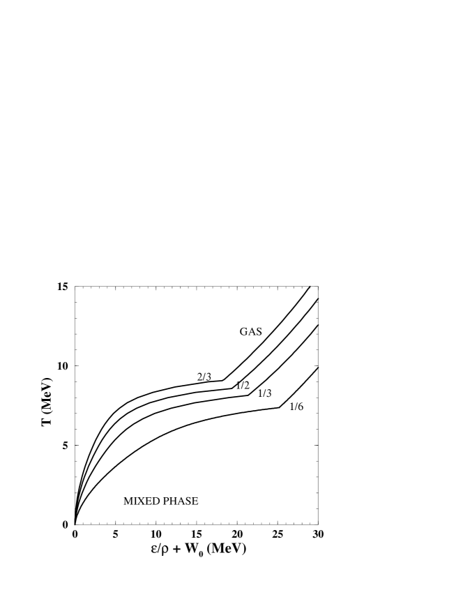
FIG. 7.: Temperature as a function of energy density per nucleon (caloric curve) is shown for fixed nucleon densities ${\rho}/{\rho_{\rm o}}=1/6,1/3,1/2,2/3$.

FIG. 8.: Specific heat per nucleon as a function of temperature at fixed nucleon density ${\rho}/{\rho_{\rm o}}=1/3$. The dashed line shows the finite discontinuity of $c_{\rho}(T)$ at the boundary of the mixed and gaseous phases. The negative specific heat appears in the vicinity of $T=18$ MeV.

FIG. 9.: Phase diagrams in $T-\rho$ plane for $\tau=3.6$ (upper panel) and $\tau=2.6$ (lower panel). Point $C$ in the lower panel is the tricritical point. Crosses correspond to the liquid phase of the first order phase transition and dots correspond to the states of the second order one.

Contributions on

Chiral Quark Models and Astrophysics

On the $\eta$–$\eta^{\prime}$ Complex in the SD–BS Approach

D. Klabucar^†, D. Kekez^‡ and M. D. Scadron^∗

^† Physics Department, Faculty of Science, University of Zagreb,
Bijenicka c. 32, Zagreb 10000, Croatia
^‡ Rudjer Bosković Institute, P.O.B. 180, 10002 Zagreb, Croatia
^∗ Physics Department, University of Arizona, Tucson, AZ 85721, USA

A $\eta$–$\eta^{\prime}$ phenomenology and Goldstone structure

The physical isoscalar pseudoscalars $\eta$ and $\eta^{\prime}$ are usually given as

$$|\eta\rangle=\cos\theta\,|\eta_{8}\rangle-\sin\theta\,|\eta_{0}\rangle~{},\,\,\,\,\,\,\,|\eta^{\prime}\rangle=\sin\theta\,|\eta_{8}\rangle+\cos\theta\,|\eta_{0}\rangle~{},$$ (1)

i.e., as the orthogonal mixture of the respective octet and singlet isospin zero states, $\eta_{8}$ and $\eta_{0}$. In the flavor SU(3) quark model, they are defined through quark–antiquark ($q\bar{q}$) basis states $|f\bar{f}\rangle$ ($f=u,d,s$) as

$$|\eta_{8}\rangle = \frac{1}{\sqrt{6}}(|u\bar{u}\rangle+|d\bar{d}\rangle-2|s\bar{s}\rangle)~{},$$ (3)

$$|\eta_{0}\rangle = \frac{1}{\sqrt{3}}(|u\bar{u}\rangle+|d\bar{d}\rangle+|s\bar{s}\rangle)~{}.$$ (4)

The exact SU(3) flavor symmetry ($m_{u}=m_{d}=m_{s}$) is nevertheless badly broken. It is an excellent approximation to assume the exact isospin symmetry ($m_{u}=m_{d}$), and a good approximation to take even the chiral symmetry limit for $u$ and $d$-quark (where current quark masses $m_{u}=m_{d}=0$), but for a realistic description, the strange quark mass $m_{s}$ must be significantly heavier than $m_{u}$ and $m_{d}$. The same holds for the constituent quark masses, denoted by $\hat{m}$ for both $u$ and $d$ quarks since we rely on the isosymmetric limit, and by $\hat{m}_{s}$ for the $s$-quark. They are nonvanishing in the chiral limit (CL). In the strange sector, CL is useful only qualitatively, as a theoretical limit. (CL would reduce $\hat{m}_{s}$ to $\hat{m}$, on which CL has almost negligible influence.)

Thus, with $|u\bar{u}\rangle$ and $|d\bar{d}\rangle$ being practically chiral states as opposed to a significantly heavier $|s\bar{s}\rangle$, Eqs. (1) do not define the octet and singlet states of the exact SU(3) flavor symmetry, but the effective octet and singlet states. Hence, as in Ref. [2] for example, only in the sense that the same $q\bar{q}$ states $|f\bar{f}\rangle$ ($f=u,d,s$) appear in both Eq. (3) and Eq. (4) do these equations implicitly assume nonet symmetry (as pointed out by Gilman and Kauffman [3], following Chanowitz, their Ref. [8]). However, in order to avoid the U_A(1) problem, this symmetry must ultimately be broken at least at the level of the masses. In particular, it must be broken in such a way that $\eta\to\eta_{8}$ becomes massless but $\eta^{\prime}\to\eta_{0}$ remains massive (as in Ref. [2]) when CL is taken for all three flavors, $m_{u},m_{d},m_{s}\to 0$. Nevertheless, the CL-vanishing octet eta mass $m_{\eta_{8}}$ is rather heavy for the realistically broken SU(3) flavor symmetry; for the empirical pion and kaon masses $m_{\pi}$ and $m_{K}$, the Gell-Mann-Okubo mass formula $m_{\pi}^{2}+3m_{\eta_{8}}^{2}=4m_{K}^{2}$ yields $m_{\eta_{8}}\approx 567$ MeV. In that case, and for the empirical masses of $\eta(547)$ and $\eta^{\prime}(958)$, the singlet $\eta_{0}$ mass $m_{\eta_{0}}$ (nonvanishing even in CL) can be found from the mass–matrix trace

$$m_{\eta_{8}}^{2}+m_{\eta_{0}}^{2}=m_{\eta}^{2}+m_{\eta^{\prime}}^{2}\approx 1.22~{}\mbox{GeV}^{2},\hskip 7.22743pt\mbox{giving}\hskip 7.22743ptm_{\eta_{0}}\approx 947~{}\mbox{MeV}\,.$$ (5)

Alternatively, one can work in a nonstrange (NS)–strange (S) basis:

$$|\eta_{\mbox{\it NS}}\rangle = \frac{1}{\sqrt{2}}(|u\bar{u}\rangle+|d\bar{d}\rangle)=\frac{1}{\sqrt{3}}|\eta_{8}\rangle+\sqrt{\frac{2}{3}}|\eta_{0}\rangle~{},$$ (7)

$$|\eta_{\mbox{\it S}}\rangle = |s\bar{s}\rangle=-\sqrt{\frac{2}{3}}|\eta_{8}\rangle+\frac{1}{\sqrt{3}}|\eta_{0}\rangle~{}.$$ (8)

In analogy with Eq. (5), in this basis one finds

$$m_{\eta_{NS}}^{2}+m_{\eta_{S}}^{2}=m_{\eta}^{2}+m_{\eta^{\prime}}^{2}\approx 1.22~{}\mbox{GeV}^{2},$$ (9)

whereas the NS–S mixing relations, diagonalizing the mass matrix, are

$$|\eta\rangle=\cos\phi_{P}|\eta_{\mbox{\it NS}}\rangle-\sin\phi_{P}|\eta_{\mbox{\it S}}\rangle~{},\,\,\,\,\,\,\,|\eta^{\prime}\rangle=\sin\phi_{P}|\eta_{\mbox{\it NS}}\rangle+\cos\phi_{P}|\eta_{\mbox{\it S}}\rangle~{}.$$ (10)

The singlet-octet mixing angle $\theta$, defined by Eqs. (1), is related to the NS–S mixing angle $\phi$ above as [4] $\theta=\phi-\arctan\sqrt{2}=\phi-54.74^{\circ}$.

Although mathematically equivalent to the $\eta_{8}$–$\eta_{0}$ basis, the NS–S mixing basis is more suitable for most quark model considerations, being more natural in practice when the symmetry between the NS and S sectors is broken as described in the preceding passage. There is also another important reason to keep in mind the $|{\eta_{\mbox{\it NS}}}\rangle$-$|{\eta_{S}}\rangle$ state mixing angle $\phi$. This is because it offers the quickest way to show the consistency of our procedures and the corresponding results obtained using just one ($\theta$ or $\phi$) state mixing angle, with the two-mixing-angle scheme considered in Refs. [5, 6, 7, 8, 9, 10, 11], which is defined with respect to the mixing of the decay constants. For clarification of the relationship with, and our results in the two-mixing-angle scheme, we refer to Ref. [12], particularly to its Appendix. Here, we simply note that our considerations will ultimately lead us to $\phi\approx 42^{\circ}$, practically the same as the result of Refs. [7, 8, 9, 11] and in agreement with data (e.g., see Table 2 of Feldmann’s review [11]).

FIG. 1.: Nonperturbative QCD quark annihilation illustrated by the two-gluon exchange diagram. It shows the transition of the $f\bar{f}$ pseudoscalar $P$ into the pseudoscalar $P^{\prime}$ having the flavor content $f^{\prime}{\bar{f}}^{\prime}$. The dashed lines and full circles depict the $q\bar{q}$ bound-state pseudoscalars and vertices, respectively.

As for a theoretical determination of the $\eta$–$\eta^{\prime}$ mixing angle $\phi$ or $\theta$, we follow the path of Refs. [4]. The contribution of the gluon axial anomaly to the singlet $\eta_{0}$ mass is essentially just parameterized and not really calculated, but some useful information can be obtained from the isoscalar $q\bar{q}$ annihilation graphs of which the “diamond” one in Fig. 1 is just the simplest example. That is, we can take Fig. 1 in the nonperturbative sense, where the two-gluon intermediate “states” represent any even number of gluons when forming a C⁺ pseudoscalar $\overline{q}q$ meson [13], and where quarks, gluons and vertices can be dressed nonperturbatively, and possibly include gluon configurations such as instantons. Factorization of the quark propagators in Fig. 1 characterized by the ratio $X\approx\hat{m}/\hat{m}_{s}$ leads to the $\eta$–$\eta^{\prime}$ mass matrix in the NS–S basis [4]

$$\left(\begin{array}[]{ll}m_{\pi}^{2}+2\beta&\,\,\,\,\quad\sqrt{2}\beta X\\ \,\,\sqrt{2}\beta X&\,2m_{K}^{2}-m_{\pi}^{2}+\beta X^{2}\end{array}\right)\begin{array}[]{c}\vspace{-2mm}\longrightarrow\\ \phi\end{array}\left(\begin{array}[]{ll}m_{\eta}^{2}&0\\ 0&m_{\eta^{\prime}}^{2}\end{array}\right),$$ (11)

where $\beta$ denotes the total annihilation strength of the pseudoscalar $q\bar{q}$ for the light flavors $f=u,d$, whereas it is assumed attenuated by a factor $X$ when a $s\bar{s}$ pseudoscalar appears. (The mass matrix in the $\eta_{8}$-$\eta_{0}$ basis reveals that in the $X\to 1$ limit, the CL-nonvanishing singlet $\eta_{0}$ mass is given by $3\beta$.) The two parameters on the left-hand-side (LHS) of (11), $\beta$ and $X$, are determined by the two diagonalized $\eta$ and $\eta^{\prime}$ masses on the RHS of (11). The trace and determinant of the matrices in (11) then fix $\beta$ and $X$ to be [4]

$$\beta=\frac{(m_{\eta^{\prime}}^{2}-m_{\pi}^{2})(m_{\eta}^{2}-m_{\pi}^{2})}{4(m_{K}^{2}-m_{\pi}^{2})}\approx 0.28~{}\mbox{GeV}^{2}~{}~{},\hskip 21.68121ptX\approx 0.78~{},$$ (12)

with the latter value suggesting a S/NS constituent quark mass ratio $X^{-1}\sim\hat{m}_{s}/\hat{m}\sim 1.3$ , near the values in Refs. [13, 14, 15, 16, 17], $\hat{m}_{s}/\hat{m}\approx 1.45$.

This fitted nonperturbative scale of $\beta$ in (12) depends only on the gross features of QCD. If instead one treats the QCD graph of Fig. 1 in the perturbative sense of literally two gluons exchanged, then one obtains [18] only $\beta_{2g}\sim 0.09~{}\mbox{GeV}^{2}$, which is about $1/3$ of the needed scale of $\beta$ found in (12). (This indicates that just the perturbative “diamond” graph can hardly represent even the roughest approximation to the effect of the gluon axial anomaly operator $\epsilon^{\alpha\beta\mu\nu}G^{a}_{\alpha\beta}G^{a}_{\mu\nu}$.) The above fitted quark annihilation (nonperturbative) scale $\beta$ in (12) can be converted to the NS–S $\eta$–$\eta^{\prime}$ mixing angle $\phi$ in (10) from the alternative mixing relation $\tan 2\phi=2\sqrt{2}\beta X(m_{\eta_{S}}^{2}-m_{\eta_{NS}}^{2})^{-1}\approx 9.02$ to [4]

$$\phi=\arctan\left[\frac{(m_{\eta^{\prime}}^{2}-2m_{K}^{2}+m_{\pi}^{2})(m_{\eta}^{2}-m_{\pi}^{2})}{(2m_{K}^{2}-m_{\pi}^{2}-m_{\eta}^{2})(m_{\eta^{\prime}}^{2}-m_{\pi}^{2})}\right]^{1/2}\approx 41.84^{\circ}~{}.$$ (13)

This kinematical QCD mixing angle (13) or $\theta=\phi-54.74^{\circ}\approx-12.9^{\circ}$ has dynamical analogs [2, 12], namely the coupled SD-BS approach discussed below, in Sec. B. Since this predicted $\eta$–$\eta^{\prime}$ mixing angle in (13) is compatible with the values repeatedly extracted in various empirical ways [14, 15], and more recently from the FKS scheme and theory [7, 8, 9, 10, 11], we confidently use the value (13) in the mixing angle relations (10) to infer the nonstrange and strange $\eta$ masses,

$$m_{\eta_{NS}}^{2} = \cos^{2}\phi~{}m_{\eta}^{2}+\sin^{2}\phi~{}m_{\eta^{\prime}}^{2}\approx(757.9~{}\mbox{MeV})^{2}$$ (15)

$$m_{\eta_{S}}^{2} = \sin^{2}\phi~{}m_{\eta}^{2}+\cos^{2}\phi~{}m_{\eta^{\prime}}^{2}\approx(801.5~{}\mbox{MeV})^{2}~{}~{}.$$ (16)

Thus it is clear that the true physical masses $\eta(547)$ and $\eta^{\prime}(958)$ are respectively much closer to the Nambu-Goldstone (NG) octet $\eta_{8}(567)$ and the non-NG singlet $\eta_{0}(947)$ configurations than to the nonstrange $\eta_{\mbox{\it NS}}(758)$ and strange $\eta_{S}(801)$ configurations inferred in Eqs. (13). However, the mean $\eta$–$\eta^{\prime}$ mass $(548+958)/2\approx 753~{}\mbox{MeV}$ is quite near the nonstrange $\eta_{\mbox{\it NS}}(758)$. But since $\eta_{8}(567)$ appears far from the NG massless limit we must ask: how close is $\eta_{0}(947)$ to the chiral-limiting nonvanishing singlet $\eta$ mass?

To answer this latter question, return to Fig. 1 and the quark annihilation strength $\beta\approx 0.28$ GeV² in Eq. (12). These $\overline{q}q$ states presumably hadronize into the U_A(1) singlet state (4), for effective squared mass in the SU(3) limit with $\beta$ remaining unchanged [18]:

$$m^{2}_{\eta_{0}}=3\beta\approx(917~{}\mbox{MeV})^{2}~{}.$$ (17)

This latter CL $\eta_{0}$ mass in (17) is only 3% shy of the exact chiral-broken $\eta_{0}(947)$ mass found in Eq. (5). (Such a 3% CL reduction also holds for the pion decay constant $f_{\pi}\approx 93$ MeV $\to 90$ MeV [19] and for $f_{+}(0)=1\to 0.97$ [20], the $K$–$\pi$ $K_{l3}$ form factor.)

Our $\eta$–$\eta^{\prime}$ mixing analysis on the basis of phenomenological mass inputs thus tells us that the physical $\eta(547)$ is 97% of the chiral-broken NG boson $\eta_{8}(567)$. Also the mixing-induced CL singlet mass of 917 MeV in (17) is 97% of the chiral-broken singlet $\eta_{0}(947)$ in (5), which in turn is 99% of the physical $\eta^{\prime}$ mass $\eta^{\prime}(958)$. This can be viewed as the phenomenological resolution of the U_A(1) problem of the masses and (quasi-)Goldstone boson structure of the observed $\eta(547)$ and $\eta^{\prime}(958)$ mesons. Or rather, from a more microscopic standpoint, the above represents phenomenological constraints that microscopic, more or less QCD–based studies of the $\eta$–$\eta^{\prime}$ complex must respect.

B Bound-state SD–BS approach to $\eta$–$\eta^{\prime}$

The coupled Schwinger-Dyson (SD) and Bethe-Salpeter (BS) approach [21] can be formulated so that it has strong and clear connections with QCD, the fundamental theory of strong interactions. In this approach, by solving the SD equation for dressed quark propagators of various flavors, one explicitly constructs constituent quarks. They in turn build $q\bar{q}$ meson bound states which are solutions of the BS equation employing the dressed quark propagator obtained as the solution of the SD equation. If the SD and BS equations are so coupled in a consistent approximation, the light pseudoscalar mesons are simultaneously the $q\bar{q}$ bound states and the (quasi) Goldstone bosons of dynamical chiral symmetry breaking (D$\chi$SB). The resulting relativistically covariant bound-state model (such as the variant of Ref. [22]) is consistent with current algebra because it incorporates the correct chiral symmetry behavior thanks to D$\chi$SB obtained in an, essentially, Nambu–Jona-Lasinio fashion, but the SD–BS model interaction is less schematic. In Refs. [2, 22, 23, 24, 25, 26] for example, it is combined nonperturbative and perturbative gluon exchange; the effective propagator function is the sum of the known perturbative QCD contribution and the modeled nonperturbative component. For details, we refer to Refs. [2, 22, 23, 24, 25], while here we just note that the momentum-dependent dynamically generated quark mass functions ${\cal M}_{f}(q^{2})$ (i.e., the quark propagator SD solutions for quark flavors $f$) illustrate well how the coupled SD-BS approach provides a modern constituent model which is consistent with perturbative and nonperturbative QCD. For example, the perturbative QCD part of the gluon propagator leads to the deep Euclidean behaviors of quark propagators (for all flavors) consistent with the asymptotic freedom of QCD [24]. However, what is important in the present paper, is the behavior of the mass functions ${\cal M}_{f}(q^{2})$ for low momenta [$q^{2}=0$ to $-q^{2}\approx(400\,{\rm MeV})^{2}$], where ${\cal M}_{f}(q^{2})$ (due to D$\chi$SB) has values consistent with typical values of the constituent mass parameter in constituent quark models. For the (isosymmetric) $u$- and $d$-quarks, our concrete model choice [22] gives us ${\cal M}_{u,d}(0)=356$ MeV in the chiral limit (i.e., with vanishing ${\widetilde{m}}_{u,d}$, the explicit chiral symmetry breaking bare mass term in the quark propagator SD equation, resulting in vanishing pion mass eigenvalue, $m_{\pi}=0$, in the BS equation), and ${\cal M}_{u,d}(0)=375$ MeV [just 5% above ${\cal M}_{u,d}(0)$ in the chiral limit] with the bare mass ${\widetilde{m}}_{u,d}=3.1$ MeV, leading to a realistically light pion, $m_{\pi}=140.4$ MeV. Similarly, for the $s$ quark, ${\cal M}_{s}(0)=610$ MeV. The simple-minded constituent masses in both NS and S sectors, $\hat{m}$ and $\hat{m}_{s}$ employed in Sec. A, have thus close analogues in the coupled SD–BS approach which explicitly incorporates some crucial features of QCD, notably D$\chi$SB. Thanks to D$\chi$SB, this dynamical, bound-state approach successfully incorporates the partially Goldstone boson structure of the mixed $\eta(547)$ and $\eta^{\prime}(958)$ mesons [2].

Before addressing its mass matrix, let us briefly recall what the SD–BS approach revealed [2, 12] about the mixing angle inferred from $\eta,\eta^{\prime}\to\gamma\gamma$ decays. The SD–BS approach incorporates the correct chiral symmetry behavior thanks to D$\chi$SB and is consistent with current algebra. Therefore, and this gives particular weight to the constraints placed on the mixing angle $\theta$ by the SD-BS results on $\gamma\gamma$ decays of pseudoscalars, this approach reproduces (when care is taken to preserve the vector Ward-Takahashi identity of QED) analytically and exactly the CL pseudoscalar $\to\gamma\gamma$ decay amplitudes (e.g., $\pi^{0}\to\gamma\gamma$), which are fixed by the Abelian axial anomaly. (Note that they are otherwise notoriously difficult to reproduce in bound-state approaches, as discussed in Ref. [24].)

General and robust considerations in this chirally well-behaved approach showed [2] that, unlike the pion case, $\eta_{8},\eta_{0}\to\gamma\gamma$ (and therefore also their mixtures $\eta,\eta^{\prime}\to\gamma\gamma$) decay amplitudes cannot be given through their respective axial-current decay constants $f_{\eta_{8}},f_{\eta_{0}}$, and also gave strong bounds on these amplitudes with respect to the pion decay constant $f_{\pi}$ (i.e., w. r. to the $\pi^{0}\to\gamma\gamma$ amplitude). All this says that in models relying on quark degrees of freedom, reasonably accurate reproduction of the empirical $\eta,\eta^{\prime}\to\gamma\gamma$ widths is possible only for $\theta$-values less negative than $-15^{\circ}$. For the concrete [23, 22] model adopted in Ref. [2], our calculated $\eta,\eta^{\prime}\to\gamma\gamma$ widths fit the data best for $\theta=-12.0^{\circ}$.

For the very predictive SD-BS approach to be consistent, the above mixing angle extracted from $\eta,\eta^{\prime}\to\gamma\gamma$ widths, should be close to the angle $\theta$ predicted by diagonalizing the $\eta$–$\eta^{\prime}$ mass matrix. In this section, it is given in the quark $f\bar{f}$ basis:

$${\hat{M}}^{2}=\mbox{\rm diag}(M_{u\bar{u}}^{2},M_{d\bar{d}}^{2},M_{s\bar{s}}^{2})+\beta\left(\begin{array}[]{ccl}1&1&1\\ 1&1&1\\ 1&1&1\end{array}\right)~{}.$$ (18)

As in Sec. A, $3\beta$ (called $\lambda_{\eta}$ in Ref. [2]) is the contribution of the gluon axial anomaly to $m_{\eta_{0}}^{2}$, the squared mass of $\eta_{0}$. We denote by $M_{f{\bar{f}}^{\prime}}$ the masses obtained as eigenvalues of the BS equations for $q\bar{q}$ pseudoscalars with the flavor content ${f{\bar{f}}^{\prime}}$ ($f,f^{\prime}=u,d,s$). However, since Ref. [2] had to employ a rainbow-ladder approximation (albeit the improved one of Ref. [22]), it could not calculate the gluon axial anomaly contribution $3\beta$. It could only avoid the U_A(1)-problem in the $\eta$–$\eta^{\prime}$ complex by parameterizing $3\beta$, namely that part of the $\eta_{0}$ mass squared which remains nonvanishing in the CL. Because of the rainbow-ladder approximation (which does not contain even the simplest annihilation graph – Fig. 1), the $q\bar{q}$ pseudoscalar masses $M_{f{\bar{f}}^{\prime}}$ do not contain any contribution from $3\beta$, unlike the nonstrange and strange $\eta$ masses $m_{\eta_{NS}}$ [in Eq. (15)] and $m_{\eta_{S}}$ [in Eq. (16)], which do, and which must not be confused with $M_{u\bar{u}}=M_{d\bar{d}}$ and $M_{s\bar{s}}$. Since the flavor singlet gluon anomaly contribution $3\beta$ does not influence the masses $m_{\pi}$ and $m_{K}$ of the non-singlet pion and kaon, the realistic rainbow-ladder modeling aims directly at reproducing the empirical values of these masses: $M_{u\bar{u}}=M_{d\bar{d}}=m_{\pi}$ and $M_{s\bar{d}}=m_{K}$. In contrast, the masses of the physical etas, $m_{\eta}$ and $m_{\eta^{\prime}}$, must be obtained by diagonalizing the $\eta_{8}$-$\eta_{0}$ sub-matrix containing both $M_{f\bar{f}}$ and the gluon anomaly contribution to $m_{\eta_{0}}^{2}$.

Since the gluon anomaly contribution $3\beta$ vanishes in the large $N_{c}$ limit as $1/N_{c}$, while all $M_{f{\bar{f}}^{\prime}}$ vanish in CL, our $q\bar{q}$ bound-state pseudoscalar mesons behave in the $N_{c}\to\infty$ and chiral limits in agreement with QCD and $\chi$PT (e.g., see [27]): as the strict CL is approached for all three flavors, the SU(3) octet pseudoscalars including $\eta$ become massless Goldstone bosons, whereas the chiral-limit-nonvanishing $\eta^{\prime}$-mass $3\beta$ is of order $1/N_{c}$ since it is purely due to the gluon anomaly. If one lets $3\beta\to 0$ (as the gluon anomaly contribution behaves for $N_{c}\to\infty$), then for any quark masses and resulting $M_{f\bar{f}}$ masses, the “ideal” mixing ($\theta=-54.74^{\circ}$) takes place so that $\eta$ consists of $u,d$ quarks only and becomes degenerate with $\pi$, whereas $\eta^{\prime}$ is the pure $s\bar{s}$ pseudoscalar bound state with the mass $M_{s\bar{s}}$.

In Ref. [2], numerical calculations of the mass matrix were performed for the realistic chiral and SU(3) symmetry breaking, with the finite quark masses (and thus also the finite BS $q\bar{q}$ bound-state pseudoscalar masses $M_{f\bar{f}}$) fixed by the fit [22] to static properties of many mesons but excluding the $\eta$–$\eta^{\prime}$ complex. The mixing angle which diagonalizes the $\eta_{8}$-$\eta_{0}$ mass matrix thus depended in Ref. [2] only on the value of the additionally introduced “gluon anomaly parameter” $3\beta$. Its preferred value turned out to be $3\beta=1.165$ GeV²=(1079 MeV)², leading to the mixing angle $\theta=-12.7^{\circ}$ [compatible with $\phi=41.84^{\circ}$ in Eq. (13)] and acceptable $\eta\to\gamma\gamma$ and $\eta^{\prime}\to\gamma\gamma$ decay amplitudes. Also, the $\eta$ mass was then fitted to its experimental value, but such a high value of $3\beta$ inevitably resulted in a too high $\eta^{\prime}$ mass, above 1 GeV. (Conversely, lowering $3\beta$ aimed to reduce $m_{\eta^{\prime}}$, would push $\theta$ close to $-20^{\circ}$, making predictions for $\eta,\eta^{\prime}\to\gamma\gamma$ intolerably bad.) However, unlike Eq. (11) in the present paper, it should be noted that Ref. [2] did not introduce into the mass matrix the “strangeness attenuation parameter” $X$ which should suppress the nonperturbative quark $f\bar{f}\to f^{\prime}{\bar{f}}^{\prime}$ annihilation amplitude (illustrated by the “diamond” graph in Fig. 1) when $f$ or $f^{\prime}$ are strange. Ref. [12] concluded that it was precisely the lack of the strangeness attenuation factor $X$ that prevented Ref. [2] from satisfactorily reproducing the $\eta^{\prime}$ mass when it successfully did so with the $\eta$ mass and $\gamma\gamma$ widths.

One can expect that the influence of this suppression should be substantial, since $X\approx{\hat{m}}/\hat{m}_{s}$ should be a reasonable estimate of it, and this nonstrange-to-strange constituent mass ratio in the considered variant of the SD-BS approach [2] is not far from $X$ in Eq. (12) and from the mass ratios in Refs. [13, 16, 17], and is even closer to the mass ratios in the Refs. [15]. Namely, two of us found [2] it to be around ${\cal M}_{u}(0)/{\cal M}_{s}(0)=0.615$ if the constituent mass was defined at the vanishing argument $q^{2}$ of the momentum-dependent SD mass function ${\cal M}_{f}(q^{2})$.

We therefore introduce the suppression parameter $X$ the same way as in the NS–S mass matrix (11), whereby the mass matrix in the $f\bar{f}$ basis becomes

$${\hat{M}}^{2}=\mbox{\rm diag}(M_{u\bar{u}}^{2},M_{d\bar{d}}^{2},M_{s\bar{s}}^{2})+\beta\left(\begin{array}[]{ccl}1&1&X\\ 1&1&X\\ X&X&X^{2}\end{array}\right)~{}.$$ (19)

The very accurate isospin symmetry makes the mixing of the isovector $\pi^{0}$ and the isoscalar etas negligible for all our practical purposes. Going to a meson basis of $\pi^{0}$ and etas enables us therefore to separate the $\pi^{0}$ and restrict ${\hat{M}}^{2}$ to the $2\times 2$ subspace of the etas. In the NS–S basis,

$$\left(\begin{array}[]{ll}m_{\eta_{NS}}^{2}&m_{\eta_{S}\eta_{NS}}^{2}\\ m_{\eta_{NS}\eta_{S}}^{2}&m_{\eta_{S}}^{2}\end{array}\right)=\left(\begin{array}[]{ll}M_{u\bar{u}}^{2}+2\beta&\quad\sqrt{2}\beta X\\ \,\sqrt{2}\beta X&M_{s\bar{s}}^{2}+\beta X^{2}\end{array}\right).$$ (20)

To a very good approximation, Eq. (20) recovers Eq. (11). This is because not only $m_{\pi}=M_{u\bar{u}}=M_{d\bar{d}}$, but also because $M_{s\bar{s}}^{2}$ differs from $2m_{K}^{2}-m_{\pi}^{2}$ only by a couple of percent, thanks to the good chiral behavior of the masses $M_{f{\bar{f}}^{\prime}}$ calculated in SD-BS approach. (These $M_{f\bar{f}^{\prime}}^{2}$ and the CL model values of $f_{\pi}$ and quark condensate, satisfy Gell-Mann-Oakes-Renner relation to first order in the explicit chiral symmetry breaking [23].) The SD-BS–predicted octet (quasi-)Goldstone masses $M_{f{\bar{f}}^{\prime}}$ are known to be empirically successful in our concrete model choice [22], but the question is whether the SD-BS approach can also give some information on the $X$-parameter. If we treat both $3\beta$ and $X$ as free parameters, we can of course fit both the $\eta$ mass and the $\eta^{\prime}$ mass to their experimental values. For the model parameters as in Ref. [22] (for these parameters our independent calculation gives $m_{\pi}=M_{u\bar{u}}=140.4$ MeV and $M_{s\bar{s}}=721.4$ MeV), this happens at $3\beta=0.753$ GeV² =(868 MeV)² and $X=0.835$. However, the mixing angle then comes out as $\theta=-17.9^{\circ}$, which is too negative to allow consistency of the empirically found two-photon decay amplitudes of $\eta$ and $\eta^{\prime}$, with predictions of our SD-BS approach for the two-photon decay amplitudes of $\eta_{8}$ and $\eta_{0}$ [2].

Therefore, and also to avoid introducing another free parameter in addition to $3\beta$, we take the path where the dynamical information from our SD-BS approach is used to estimate $X$. Namely, our $\gamma\gamma$ decay amplitudes $T_{f\bar{f}}$ can be taken as a serious guide for estimating the $X$-parameter instead of allowing it to be free. We did point out in Sec. A that the attempted treatment [18] of the gluon anomaly contribution through just the “diamond diagram” contribution to $3\beta$, indicated that just this partial contribution is quite insufficient. This limits us to keeping $3\beta$ as a free parameter, but we can still suppose that this diagram can help us get the prediction of the strange-nonstrange ratio of the complete pertinent amplitudes $f\bar{f}\to f^{\prime}{\bar{f}}^{\prime}$ as follows. Our SD-BS modeling in Ref. [2] employs an infrared-enhanced gluon propagator [22, 24] weighting the integrand strongly for low gluon momenta squared. Therefore, in analogy with Eq. (4.12) of Kogut and Susskind [28] (see also Refs. [29, 30]), we can approximate the Fig. 1 amplitudes $f\bar{f}\to{\rm 2gluons}\to f^{\prime}{\bar{f}}^{\prime}$, i.e., the contribution of the quark-gluon diamond graph to the element $ff^{\prime}$ of the $3\times 3$ mass matrix, by the factorized form

$${\widetilde{T}}_{f\bar{f}}(0,0)\,{\cal C}\,\,{\widetilde{T}}_{f^{\prime}{\bar{f}}^{\prime}}(0,0)\,.$$ (21)

In Eq. (21), the quantity ${\cal C}$ is given by the integral over two gluon propagators remaining after factoring out ${\widetilde{T}}_{f\bar{f}}(0,0)$ and ${\widetilde{T}}_{f^{\prime}{\bar{f}}^{\prime}}(0,0)$, the respective amplitudes for the transition of the $q\bar{q}$ pseudoscalar bound state for the quark flavor $f$ and $f^{\prime}$ into two vector bosons, in this case into two gluons. The contribution of Fig. 1 is thereby expressed with the help of the (reduced) amplitudes ${\widetilde{T}}_{f\bar{f}}(0,0)$ calculated in Ref. [2] for the transition of $q\bar{q}$ pseudoscalars to two real photons ($k^{2}={k^{\prime}}^{2}=0$), while in general ${\widetilde{T}}_{f\bar{f}}(k^{2},k^{\prime 2})\equiv{T}_{f\bar{f}}(k^{2},k^{\prime 2})/Q_{f}^{2}$ are the “reduced” two-photon amplitudes obtained by removing the squared charge factors $Q_{f}^{2}$ from ${T}_{f\bar{f}}$, the $\gamma\gamma$ amplitude of the pseudoscalar $q\bar{q}$ bound state of the hidden flavor $f{\bar{f}}$. Although ${\cal C}$ is in principle computable, all this unfortunately does not amount to determining $\beta,\beta X$ and $\beta X^{2}$ in Eq. (19) since the higher (four-gluon, six-gluon, … , etc.) contributions are clearly lacking. We therefore must keep the total (light-)quark annihilation strength $\beta$ as a free parameter. However, if we assume that the suppression of the diagrams with the strange quark in a loop is similar for all of them, Eq. (21) and the “diamond” diagram in Fig. 1 help us to at least estimate the parameter $X$ as $X\approx{\widetilde{T}}_{s\bar{s}}(0,0)/{\widetilde{T}}_{u\bar{u}}(0,0)$. This is a natural way to build in the effects of the SU(3) flavor symmetry breaking in the $q\bar{q}$ annihilation graphs. (Recall that ${\widetilde{T}}_{s\bar{s}}(0,0)/{\widetilde{T}}_{u\bar{u}}(0,0)\approx\hat{m}/\hat{m}_{s}$ to a good approximation [12].)

We get $X=0.663$ from the two-photon amplitudes we obtained in the chosen SD-BS model [22]. This value of $X$ agrees well with the other way of estimating $X$, namely the nonstrange-to-strange constituent mass ratio of Refs. [13, 16, 17]. With $X=0.663$, requiring that the $2\times 2$ matrix trace, $m_{\eta}^{2}+m_{\eta^{\prime}}^{2}$, be fitted to its empirical value, fixes the chiral-limiting nonvanishing singlet mass squared to $3\beta=0.832$ GeV²=(912 MeV)², just 0.5% below Eq. (17), while $m_{\eta_{NS}}=757.87$ MeV and $m_{\eta_{S}}=801.45$ MeV, practically the same as Eqs. (13). The resulting mixing angle and $\eta$, $\eta^{\prime}$ masses are

$$\phi=41.3^{\circ}\hskip 7.22743pt\mbox{or}\hskip 7.22743pt\theta=-13.4^{\circ}\,\,;\quad m_{\eta}=588\,\mbox{MeV}\,,\quad m_{\eta^{\prime}}=933\,\mbox{MeV}\,.$$ (22)

These results are for the original parameters of Ref. [2]. Reference [12] also varied the parameters to check the sensitivity on SD-BS modeling, but the results changed little.

The above results of the SD-BS approach [2] are very satisfactory since they agree very well with what was found in Sec. A by different methods. They also agree with the UKQCD lattice results [31] on $\eta$–$\eta^{\prime}$ mixing. Their calculated mixing parameter $x_{ss}$ corresponds to our $\beta X^{2}$, and their mixing parameters $x_{nn}$ and $x_{ns}$ ($n=u,d$), corresponding respectively to our $\beta$ and $\beta X$, are aimed to obey $x_{nn}\approx 2x_{ss}$ and $x_{ns}^{2}\approx x_{nn}x_{ss}$. UKQCD prefers [31] $x_{ss}=0.13$ GeV², $x_{nn}=0.292$ GeV² and $x_{ns}=0.218$ GeV². This, together with their preferred input values $M_{n\bar{n}}=0.137$ GeV and $M_{s\bar{s}}=0.695$ GeV, give the NS–S mass matrix (20) with elements reasonably close to ours, resulting in a rather close mixing angle, $\theta=-10.2^{\circ}$.

C Conclusion

We have shown that the treatment of the $\eta$–$\eta^{\prime}$ complex in the SD–BS approach [2] is sensible in spite of employing the ladder approximation. This is confirmed especially by Ref. [12] which showed its connection and robust agreement with the phenomenological studies of the $\eta$–$\eta^{\prime}$ complex. It is therefore desirable to extend the SD–BS studies of the $\eta$–$\eta^{\prime}$ mass matrix to finite temperatures. Usually, one has neglected all temperature dependences in the mass matrix, except the one of the gluon anomaly contribution $3\beta$ which is assumed very strong, which is appropriate if the U_A(1) symmetry breaking is due to instantons [32, 33, 34, 35]. However, rather strong topological arguments of Kogut et al. [36] that the U_A(1) symmetry is not restored at critical (but only at a higher, possibly infinite) $T$, motivates also the scenario where $3\beta(T)\approx const$, while other entries in the mass matrix carry the temperature dependence. The inclusion of their $T$–dependence is needed also because the scenario with the instanton–induced, strongly $T$–dependent $\beta$ should be carefully re-examined, since it has lead to contradicting conclusions: the depletion of $\eta^{\prime}$ production in Ref. [33], but $\eta^{\prime}$–enhancement in Ref. [34].

The temperature dependence of $m_{\pi}=M_{u\bar{u}}=M_{d\bar{d}}$, ${\cal M}_{u,d}(q^{2})$, $f_{\pi}$ and $\langle{u\bar{u}}\rangle(=\langle{d\bar{d}}\rangle)$, was already studied in various SD–BS models [37, 38], so that the extension [39] to the $T$–dependence of the remaining needed ingredients, $M_{s\bar{s}}$, ${\cal M}_{s}(q^{2})$, $f_{s\bar{s}}$ and $\langle{s\bar{s}}\rangle$, should be straightforward.

Acknowledgments: D. Kl. thanks D. Blaschke, S. Schmidt and G. Burau, the organizers of the workshop “Quark Matter in Astro- and Particle Physics” (27.-29. November 2000, Rostock, Germany) for their hospitality and for the support which made his participation possible.

Pseudoscalar mesons in asymmetric matter

Maria C. Ruivo, Pedro Costa and Célia A. de Sousa

Centro de Física Teórica, Departamento de Física
Universidade de Coimbra P - 3004 - 516 Coimbra, Portugal

A Introduction

During the last few years, major experimental and theoretical efforts have been dedicated to heavy-ion collisions aiming at understanding the properties of hot and dense matter and looking for signatures of phase transitions to the quark-gluon plasma. As a matter of fact, it is believed that, at critical values of the density, $\rho_{c}$, and/or temperature, $T_{c}$, the system undergoes a phase transition, the QCD vacuum being then described by a weakly interacting gas of quarks and gluons, with restored chiral symmetry.

The nature of the phase transition is an important issue nowadays. Lattice simulations [1] provide information at zero density and finite temperature but for finite densities no firm lattice results are available and most of our knowledge comes from model calculations. The Nambu-Jona-Lasinio[2] [NJL] type models have been extensively used over the past years to describe low energy features of hadrons and also to investigate restoration of chiral symmetry with temperature or density [3, 23, 6, 5, 7].

Recently, it was shown by Buballa[14] that, with a convenient parameterization, the SU(2) and SU(3) NJL models exhibit a first order phase transition, the system being in a mixed phase between $\rho\,=\,0$ and $\rho\,=\,\rho_{c}$, the energy per particle having an absolute minimum at $\rho\,=\,\rho_{c}$. This suggests an interpretation of the model within the philosophy of the MIT bag model. The system has two phases, one consisting of droplets of quarks of high density and low mass surrounded by a non trivial vacuum and the other one consisting of a quark phase of restored chiral symmetry. Similar concepts appear in NJL inspired models including form factors [9, 10]. The physical meaning of the mesonic excitations in the medium within this interpretation of the model is an interesting subject that will be analyzed in this paper.

The possible modifications of meson properties in the medium is an important issue nowadays. The study of pseudoscalar mesons, such as kaons and pions, is particularly interesting, since, due to their Goldstone boson nature, they are intimately associated with the breaking of chiral symmetry. Since the work of Kaplan and Nelson [11], the study of medium effects on these mesons in flavor asymmetric media attracted a lot of attention. Indeed, the charge multiplets of those mesons, that are degenerated in vacuum or in symmetric matter, were predicted to have a splitting in flavor asymmetric matter. In particular, as the density increases, there would be an increase of the mass of $K^{+}$ and a decrease of the mass of $K^{-}$; a similar effect would occur for $\pi^{-}$ and $\pi^{+}$ in neutron matter. The mass decrease of one of the multiplets raises, naturally, the issue of meson condensation, a topic specially relevant to Astrophysics.

Most theoretical approaches dealing with kaons in flavor asymmetric media, predict a slight raising of the $K^{+}$ mass and a pronounced lowering of the $K^{-}$ mass [12, 5, 13, 14], a conclusion which is supported by the analysis of data on kaonic atoms [15]. Experimental results at GSI seem to be compatible with this scenario [16, 17, 18].

Studies on pions in asymmetric medium are mainly related with the problem of the $u-d$ asymmetry in a nucleon sea rich in neutrons. Such flavor asymmetry has been established in SIS and DY experiments and theoretical studies show that there is a significant difference in $\pi^{+}\,\,,\pi^{-}$ distribution functions in neutron rich matter [19].

From the theoretical point of view, the driving mechanism for the mass splitting is attributed mainly to the selective effects of the Pauli principle, although, in the case of $K^{-}$, the interaction with the $\Lambda(1405)$ resonance plays an important role as well. In the study of the effects of the medium on hadronic behavior, one should have in mind that the medium is a complex system, where a great variety of medium particle-hole excitations occur, some of them with the same quantum numbers of the hadrons under study; the interplay of all these excitations might play a significant role in the modifications of hadron properties. In previous works we have established, within the framework of NJL models, the presence, in flavor asymmetric media, of low energy pseudoscalar modes, which are excitation of the Fermi sea [4, 6]. The combined effect of density and temperature, as well as the effect of vector interaction, was discussed for the case of kaons in symmetric nuclear matter without strange quarks [5, 23].

This paper addresses the following points: a) analyzes of the phase transition with density and temperature in neutron matter in the $SU(3)$ NJL model with two different parameterizations and within the ENJL model ; b) behavior of kaonic and pionic excitations in these models and discussion of the meaning of the Fermi sea excitations, in connection with the nature of the phase transition; c) combined effect of density and temperature.

Formalism

We work in a flavor $SU(3)$ NJL type model with scalar-pseudoscalar and vector-pseudovector pieces, and a determinantal term, the ’t Hooft interaction, which breaks the $U_{A}(1)$ symmetry. We use the following Lagrangian:

$$\begin{array}[]{rcl}\cal L&=&\bar{q}\,(\,i\,{\gamma}^{\mu}\,\partial_{\mu}\,-\,\hat{m})\,q+\frac{1}{2}\,g_{S}\,\,\sum_{a=0}^{8}\,[\,{(\,\bar{q}\,\lambda^{a}\,q\,)}^{2}\,\,+\,\,{(\,\bar{q}\,i\,\gamma_{5}\,\lambda^{a}\,q\,)}^{2}\,]\\[4.0pt] &-&\frac{1}{2}\,g_{V}\,\,\sum_{a=0}^{8}\,[\,{(\,\bar{q}\,\gamma_{\mu}\,\lambda^{a}\,q\,)}^{2}\,\,+\,\,{(\,\bar{q}\gamma_{\mu}\,\gamma_{5}\,\lambda^{a}\,q\,)}^{2}\,]\\[4.0pt] &+&g_{D}\,\,\{\mbox{det}\,[\bar{q}\,(\,1\,+\,\gamma_{5}\,)\,q\,]+\mbox{det}\,[\bar{q}\,(\,1\,-\,\gamma_{5}\,)\,q\,]\,\}\\ &&\end{array}$$ (1)

In order to discuss the predictions of different models we consider the cases: $g_{V}=0$ with two parametrizations (NJL I and NJL II) and $g_{V}\neq 0$ (ENJL). The model parameters, the bare quark masses $m_{d}=m_{u},m_{s}$, the coupling constants and the cutoff in three-momentum space, $\Lambda$, are essentially fitted to the experimental values of $m_{\pi},\,f_{\pi},\,m_{K}$ and to the phenomenological values of the quark condensates, $<\bar{u}u>,\,<\bar{d}d>,\,<\bar{s}s>$. The parameter sets used are, for NJL I: $\Lambda=631.4$ MeV, $g_{S}\,\Lambda^{2}=3.658,\,g_{D}\,\Lambda^{5}=-9.40,\,m_{u}=m_{d}=5.5$ MeV and $m_{s}=132.9$ MeV; for ENJL: $\Lambda=750$ MeV, $g_{S}\,\Lambda^{2}=3.624$, $g_{D}\,\Lambda^{5}=-9.11,\,g_{V}\,\Lambda^{2}=3.842$, $m_{u}=m_{d}=3.61$ MeV and $m_{s}=88$ MeV. For NJL II we use the parametrization of [20], $\Lambda=602.3$ MeV, $g_{S}\,\Lambda^{2}=3.67$, $g_{D}\Lambda^{5}=-12.39$, $m_{u}=m_{d}=5.5$ MeV and $m_{s}=140.7$ MeV, which underestimates the pion mass ($m_{\pi}\,=135\mbox{ MeV}$) and of $\eta$ by about $6\%$.

The six quark interaction can be put in a form suitable to use the bosonization procedure (see [21, 22, 23]):

$${\cal L_{D}}\,=\,\frac{1}{6}g_{D}\,\,D_{abc}\,(\bar{q}\,{\lambda}^{c}\,q\,)\,[\,(\,\bar{q}\,\lambda^{a}\,q\,)(\bar{q}\,\lambda^{b}\,q\,)-3\,(\,\bar{q}\,i\,\gamma_{5}\,\lambda^{a}\,q\,)\,(\,\bar{q}\,i\,\gamma_{5}\,\lambda^{b}\,q\,)\,]$$ (2)

with: $D_{abc}=d_{abc}\,,a,b,c\,\,\epsilon\,\{1,2,..8\}\,,\mbox{(structure constants of SU(3))}\,,D_{000}=\sqrt{\frac{2}{3}}\,,D_{0ab}=-\sqrt{\frac{1}{6}}\delta_{ab}$.

The usual procedure to obtain a four quark effective interaction from this six quark interaction is to contract one bilinear $(\bar{q}\,\lambda_{a}\,q)$. Then, from the two previous equations, an effective Lagrangian is obtained:

$$L_{eff}\, = \bar{q}\,(\,i\,{\gamma}^{\mu}\,\partial_{\mu}\,-\,\hat{m})\,q\,\,$$ (3)

$$+ S_{ab}[\,(\,\bar{q}\,\lambda^{a}\,q\,)(\bar{q}\,\lambda^{b}\,q\,)]+\,P_{ab}[(\,\bar{q}\,i\,\gamma_{5}\,\lambda^{a}\,q\,)\,(\,\bar{q}\,i\,\gamma_{5}\,\lambda^{b}\,q\,)\,]$$ (4)

$$- \frac{1}{2}\,g_{V}\,\,\sum_{a=0}^{8}\,[\,{(\,\bar{q}\,\gamma_{\mu}\,\lambda^{a}\,q\,)}^{2}\,\,+\,\,{(\,\bar{q}\gamma_{\mu}\,\gamma_{5}\,\lambda^{a}\,q\,)}^{2}\,]\,\,$$ (5)

where:

$$S_{ab}\,=\,g_{S}\,\delta_{ab}\,+\,g_{D}D_{abc}\,<\bar{q}\,{\lambda}^{c}\,q\,>$$ (6)

$$P_{ab}\,=\,g_{S}\,\delta_{ab}\,-\,g_{D}D_{abc}\,<\bar{q}\,{\lambda}^{c}\,q\,>$$ (7)

By using the usual methods of bosonization one gets the following effective action:

$$I_{eff}= -i Tr\ {\rm ln}(\,i\,\partial_{\mu}\gamma_{\mu}-\hat{m}+\sigma_{a}\,\lambda^{a}+i\,\gamma_{5}\,{\phi}_{a}\,\,{\lambda}^{a}\,+\,\gamma^{\mu}\,V_{\mu}\,+\gamma_{5}\,\gamma^{\mu}\,A_{\mu})$$ (8)

$$- \frac{1}{2}(\,\sigma_{a}\,{S_{ab}}^{-1}\,\sigma_{b}\,+{\phi}_{a}\,{P_{ab}}^{-1}\,\phi_{b}\,)$$ (9)

$$+ \frac{1}{2G_{V}}(\,{V^{a}_{\mu}}^{2}\,+\,{A^{a}_{\mu}}^{2}\,),$$ (10)

from which we obtain the gap equations and meson propagators.

In order to introduce the finite temperature and density, we use the thermal Green function, which, for a quark $q_{i}$ at finite temperature $T$ and chemical potential $\mu_{i}$ reads:

$$S(\vec{x}-\vec{x}^{\prime},\tau-\tau^{\prime}) = \frac{i}{\beta}{\sum}_{n}e^{-i\omega_{n}(\tau-\tau^{\prime})}$$ (11)

$$\int \frac{d^{3}p}{(2\pi)^{3}}\frac{e^{-i\,\vec{p}\,(\vec{x}-\vec{x}^{\prime})}}{\gamma_{0}(i\omega_{n}+{\overline{\mu}_{i}})-\vec{\gamma}.\vec{p}-M_{i}}\,,$$ (12)

where $\beta=1/T\,,{\overline{\mu}_{i}}\,=\,\mu_{i}\,-\,\Delta E_{i}$, $\Delta E_{i}$ is the energy gap induced by the vector interaction, $M_{i}$ the mass of the constituent quarks, $E_{i}\,=\,(p^{2}\,+\,M^{2}_{i})^{1/2}$ and $\omega_{n}\,=\,(2n+1)\,\frac{\pi}{\beta}\,\,\,,n\,=\,0\,,\pm 1\,,\pm 2\,,....,$ are the Matsubara frequencies. The following gap equations are obtained:

$$M_{i}\,=\,m_{i}\,-2\,g_{S}\,<\bar{q}_{i}\,q_{i}>\,-\,2\,g_{D}\,<\bar{q}_{j}\,q_{j}><\bar{q}_{k}\,q_{k}>$$ (13)

$$\Delta E_{i}\,=\,2\,g_{V}\,<{q_{i}}^{+}\,q_{i}>$$ (14)

with $i\,,j\,,k$ cyclic and $<\bar{q}_{i}\,q_{i}>$, $<{q_{i}}^{+}\,q_{i}>$ are respectively the quark condensates and the quark densities at finite $T$ and $\mu_{i}$.

The condition for the existence the poles in the propagators of kaons leads to the following dispersion relation:

$$(\,1\,-\,K_{P}\,\,J_{PP}\,)\,\,(\,1\,-\,K_{A}\,\,J_{AA}\,)\,-\,K_{P}\,K_{A}\,\,{J^{2}}_{PA}\,=\,0$$ (15)

with:

$$\omega\,J_{PA}\,=\,(M_{u}+M_{s})\,J_{PP}\,+\,2\,(<\bar{u}u\,>+\,<\bar{s}s>).$$

$$\omega\,J_{AA}\,=\,(M_{u}+M_{s})\,J_{PA}\,+\,2\,(<u^{+}u>\,-\,<s^{+}s>).$$

$$J_{PP}\,=\,2\,N_{c}\,\int{d^{3}p\over(2\pi)^{3}}\,\left\{\frac{M_{u}(M_{s}-M_{u})\,-q_{0}\,E_{u}}{({E_{s}}^{2}-(q_{0}+E_{u})^{2})E_{u}}\mbox{ tanh}\frac{\beta(E_{u}+{\bar{\mu}_{u})}}{2}\,+\right.$$

$$\left.\frac{M_{u}(M_{s}-M_{u})\ +q_{0}E_{u}}{({E_{s}}^{2}-(q_{0}-E_{u})^{2})E_{u}}\mbox{ tanh}\frac{\beta(E_{u}-{\bar{\mu}_{u})}}{2}\,\,+\,s\rightarrow u\,,\,q_{0}\rightarrow-q_{0}\right\}$$ (16)

with $K_{P}\,=\,g_{S}\,+\,g_{D}\,<\bar{d}d>$ and $K_{A}\,=\,-g_{V}$, ${\bar{\mu}_{u}}=\mu_{u}-\Delta E_{u}$, $q_{0}=\pm m_{K^{\pm}}-(\Delta E_{u}-\Delta E_{s})$ for $K^{\pm}$

Similar expressions are obtained for pions in neutron matter, by replacing $s\leftrightarrow d$ [6].

B Phase transitions at finite chemical potential and temperature

We reanalyze the problem of the phase transitions in order to establish a connection between the vacuum state and its excitations. We consider here the case of asymmetric quark matter without strange quarks simulating neutron matter: $\rho_{u}\,=\frac{1}{2}\,\rho_{d}\,\,,\rho_{s}\,=\,0$ and calculate the the energy and pressure. At zero temperatures we found a first order phase transition in NJL model, exhibiting different characteristics according to the parameterization used. Within the parameterization NJL I, the pressure is negative for $0.8\rho_{0}\leq\rho\leq 1.65\rho_{0}$ and the absolute minimum of the energy per particle is at $\rho=0$ (dashed curves in Fig.1).

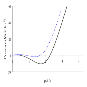
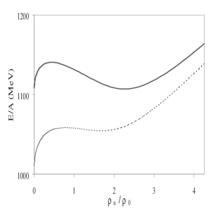
FIG. 1.: Pressure and energy per particle in NJL I (dashed curves) and NJL II (full curves).

The system, within the range of densities indicated above, is in a mixed phase consisting of droplets of massive quarks of low density and droplets of light quarks of high density and, for $\rho>1.65\rho_{0}$, is in a quark phase with partially restored chiral symmetry (in the SU(2) sector). These droplets are unstable since the absolute minimum of the energy per particle is at $\rho=0$. With parameterization II, the mixed phase starts at $\rho\simeq 0$, because, although the zeros of the pressure are at $\rho=0.44\rho_{0},\,\,\rho_{c}=2.25\rho_{0}$, the compressibility is negative in the low density region for $\rho\simeq 0$; the energy per particle has an absolute minimum at the critical density of $E/A\,=1102$ MeV, about three times the masses of the constituent non strange quarks in vacuum (Fig 1. full curves). The model may now be interpreted as having a hadronic phase — droplets of light $u\,,d$ quarks with a density $\rho_{c}=2.25\rho_{0}$ surrounded by a non trivial vacuum — and, above the critical density, a quark phase with partially restored SU(2) chiral symmetry. The model is not suitable to describe hadrons for $\rho\,<\rho_{c}$. Since there is no definition of the density in the mixed phase, we study, in the following, the mesonic excitations only for $\rho>\rho_{c}$.

The phase transition becomes second order at finite density and temperatures around $20MeV$ and also in the ENJL model, for the set of parameters chosen. In these cases the system has positive pressure but the absolute minimum of the energy per particle is at zero density. Although a gas of quarks does not exist at low densities, the model has been used to study the influence of the medium in the mesonic excitations of the vacuum. Of course, an extrapolation of quark matter to hadronic matter should be made, since we do not have, at low densities, a gas of hadrons.

C Behavior of pions and kaons in the medium

At zero temperature we observe a splitting between charge multiplets, both in NJL and ENJL models (see figs. 2-3).

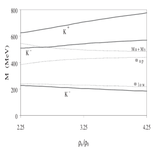
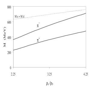
FIG. 2.: Masses of kaons and pions in NJL II. $\omega_{up}\,\mbox{and }\,\omega_{low}$ denote the limits of the Fermi sea continuum.

These modes are excitations of the Dirac sea modified by the presence of the medium. The increase of $K^{+}\mbox{and}\,\pi^{-}$ masses with respect to those of $K^{-}\,\mbox{and}\,\pi^{+}$ is due to Fermi blocking and is more pronounced for kaons than for pions because, there are $u$ and $d$ quarks in the Fermi sea and therefore there are repulsive effects due to the Pauli principle acting on $\pi^{+}$. In the case of kaons, we do not have strange quarks at these densities and so there is mora phase space available to create $\bar{u}s$ pairs of quarks and there are less repulsive effects on $K^{-}$.

An interesting feature in NJL model is that, besides these modes, low energy modes with quantum numbers of $K^{-}\,\mbox{and}\,\pi^{+}$ appear. These are particle-hole excitations of the Fermi sea which correspond to $\Lambda\,(1106)$-particle-proton-hole for kaons an to a proton-particle-neutron-hole for the case of pions. A similar effect is found for kaons in symmetric nuclear matter [6, 5]. For the case of pions, the low energy modes is less relevant and exist only for $\rho=\rho_{c}$, merging in the Fermi sea continuum afterwards. We notice that when the ’t Hooft interaction is not included [6] or in SU(2) [7] the low energy mode for pions is more relevant.

The sum rules are a very important tool to analyze the collectivity and relative importance of the modes [4, 6, 7, 5]. One can derive a generalization of the PCAC relation in the medium from the Energy Weighted Sum Rule (EWSR), well known from Many Body Theories. For the mesonic state $|r>$ with energy $\omega_{r}$ associated with the transition operator $\Gamma$ the strength function $F_{r}\,=\,\omega_{r}\,\,{|\,<\,r\,|\,\Gamma\,|\,0\,>\,|}^{2}$ satisfies the EWSR   which reads

$$m_{1}\,=\,{\sum}_{r}\,\omega_{r}\,\,{|\,<\,r\,|\,\Gamma\,|\,0\,>\,|}^{2}\,\,=\,\frac{1}{2}\,<\,\Phi_{0}\,|\,[\,\Gamma\,,\,[\,H\,,\Gamma\,]\,]\,|\,\Phi_{0}\,>,$$ (17)

the transition operator being defined in the present case by $\Gamma\,=\,\Gamma_{+}\,+\,\Gamma_{-}$, with $\Gamma_{\pm}\,=\gamma_{5}\,(\lambda_{4}\pm i\ \lambda_{5})/\sqrt{2}$, for kaons, and , $\Gamma_{\pm}\,=\gamma_{5}\,(\lambda_{1}\pm i\ \lambda_{2})/\sqrt{2}$, for pions. We obtain therefore the GMOR relation in the medium:

$$\sum_{\alpha}\,m_{K,\alpha}^{2}\,f_{K,\alpha}^{2}\,\,\simeq\,-\,\frac{1}{2}(m_{u}\,+\,m_{s}\,)\,[<\,\overline{u}\,\,u\,>\,+\,<\,\overline{s}\,\,s\,>\,]\,.$$ (18)

and

$$\sum_{\alpha}\,m_{\pi,\alpha}^{2}\,f_{\pi,\alpha}^{2}\,\,\simeq\,-\,\frac{1}{2}(m_{u}\,+\,m_{d}\,)\,[<\,\overline{u}\,\,u\,>\,+\,<\,\overline{d}\,\,d\,>\,]\,.$$ (19)

We verified that in the medium the degree of satisfaction of the sum rule is good, provided, naturally, that all the bound state solutions are considered. The strength associated to the low energy mode can not be neglected as the density increases [4, 6].

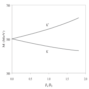
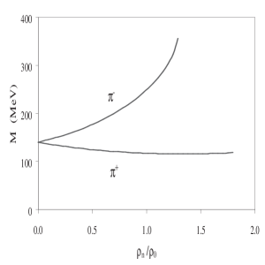
FIG. 3.: Masses of kaons and pions in ENJL model.

In the ENJL model the low energy mode does not appear, which is consistent with the fact that the analysis of the EOS shows that there is no stable Fermi sea. The attractive effects concentrate on $K^{-}\,\,,\pi^{+}$. The splitting between the charge multiplets is even larger in this model.

The influence of the temperature is, on one side, to inhibit the occurrence of the low energy mode (this mode is not seen above very low temperatures) and, on the other side, to reduce the splitting of between the upper energy modes (see Fig. 4).

We notice that temperature has an effect on the low energy mode similar to the vector pseudovector interaction in vacuum. This is meaningful since, as it has been mentioned above, as the temperature increases the phase transition is second order and the minimum of energy per particle is at $\rho=0$ and consequently the Fermi sea is not stable. So, it is reasonable that the excitations of the Fermi sea are not seen.

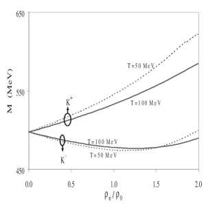
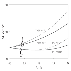
FIG. 4.: Masses of kaons and pions for $T=50$ MeV and $T=100$ MeV, in NJL II.

In conclusion, we have discussed the behavior of kaons and pions in neutron matter in NJL and ENJL model, in connection with the nature of the phase transition, at finite density with zero or non zero temperature. In the NJL model where the phase transition is first order and a stable Fermi sea exists at the critical density, we find low energy particle hole excitations of the Fermi sea, besides the usual splitting of charge multiplets which are excitations of the Dirac sea. This last effect does not occur in the ENJL model, where the transition is second order. The temperature inhibits this effect and reduces the splitting between the charge multiplets.

Acknowledgements

Work supported in part by Centro de Física Teórica, and PRAXIS/P/FIS/
12247/98, FCT, Portugal
One of us (MCR) wishes to thank finantial support from the University of Rostock, Germany.

Chiral Phase Transition in Covariant Nonlocal NJL Models

I. General^a, D. Gomez Dumm${}^{b}\ {}^{\dagger}$ and N.N. Scoccola^a,c

^a Physics Department, Comisión Nacional de Energía Atómica,
Av.Libertador 8250, (1429) Buenos Aires, Argentina
^b IFLP, Depto. de Física, Universidad Nacional de La Plata,
C.C. 67, (1900) La Plata,

Argentina
^c Universidad Favaloro, Solís 453, (1078) Buenos Aires, Argentina

A Introduction

The behaviour of hot dense hadronic matter and its transition to a plasma of quarks and gluons has received considerable attention in recent years. To a great extent this is motivated by the advent of facilities like e.g. RHIC at Brookhaven which are expected to provide some empirical information about such transition. The interest in this topic has been further increased by the recent suggestions that the QCD phase diagram could be richer than previously expected (see Ref.[1] for some recent review articles). Due to the well known difficulties to deal directly with QCD, different models have been used to study this sort of problems. Among them the Nambu-Jona-Lasinio model[2] is one of the most popular. In this model the quark fields interact via local four point vertices which are subject to chiral symmetry. If such interaction is strong enough the chiral symmetry is spontaneously broken and pseudoscalar Goldstone bosons appear. It has been shown by many authors that when the temperature and/or density increase, the chiral symmetry is restored[3]. Some covariant nonlocal extensions of the NJL model have been studied in the last few years[4]. Nonlocality arises naturally in the context of several of the most successful approaches to low-energy quark dynamics as, for example, the instanton liquid model[5] and the Schwinger-Dyson resummation techniques[6]. It has been also argued that nonlocal covariant extensions of the NJL model have several advantages over the local scheme. Namely, nonlocal interactions regularize the model in such a way that anomalies are preserved[7] and charges properly quantized, the effective interaction is finite to all orders in the loop expansion and therefore there is not need to introduce extra cut-offs, soft regulators such as Gaussian functions lead to small NLO corrections[8], etc. In addition, it has been shown[9] that a proper choice of the nonlocal regulator and the model parameters can lead to some form of quark confinement, in the sense of a quark propagator without poles at real energies. Recently, the behaviour of this kind of models at finite temperature has been investigated[10]. In this work we extend such studies to finite temperature and chemical potential.

B Non-local NJL models with separable interactions

We consider a nonlocal extension of the SU(2) NJL model defined by the effective action

$$S = \int d^{4}x\ {\bar{\psi}}(x)\left(i\hbox to0.0pt{/\hss}\partial-m_{c}\right){\psi}(x)+\int d^{4}x_{1}...d^{4}x_{4}\ V(x_{1},x_{2},x_{3},x_{4})$$ (1)

$$\!\!\!\!\!\times\!\!\! \!\!\!\!\left({\bar{\psi}}(x_{1})\psi(x_{3}){\bar{\psi}}(x_{2})\psi(x_{4})-{\bar{\psi}}(x_{1})\gamma_{5}\vec{\tau}\psi(x_{3}){\bar{\psi}}(x_{2})\gamma_{5}\vec{\tau}\psi(x_{4})\right),\!\!$$ (2)

where $m_{c}$ is the (small) current quark mass responsible for the explicit chiral symmetry breaking. The interaction kernel in Euclidean momentum space is given by

$$V(q_{1},q_{2},q_{3},q_{4})=\frac{G}{2}\ r(q_{1}^{2})r(q_{2}^{2})r(q_{3}^{2})r(q_{4}^{2})\ \delta(q_{1}\!+\!q_{2}\!-\!q_{3}\!-\!q_{4})\,,$$ (3)

where $r(q^{2})$ is a regulator normalized in such a way that $r(0)=1$. Some general forms for this regulator like Lorentzian or Gaussian functions have been used in the literature. A particular form is given in the case of instanton liquid models.

Like in the local version of the NJL model, the chiral symmetry is spontaneously broken in this nonlocal scheme for large enough values of the coupling $G$. In the Hartree approximation the self-energy $\Sigma(q^{2})$ at vanishing temperature and chemical potential is given by

$$\Sigma(q^{2})=m_{c}+(\Sigma(0)-m_{c})r^{2}(q^{2})\,,$$ (4)

where the zero-momentum self-energy $\Sigma(0)$ is a solution of the gap equation

$$\frac{2\pi^{4}}{G\ N_{c}}\left(\Sigma(0)-m_{c}\right)=\int d^{4}q\ \frac{\left[m_{c}+(\Sigma(0)-m_{c})r^{2}(q^{2})\right]r^{2}(q^{2})}{q^{2}+\left[m_{c}+(\Sigma(0)-m_{c})r^{2}(q^{2})\right]^{2}}\,.$$ (5)

In general, the quark propagator might have a rather complicate structure of poles and cuts in the complex plane. As already mentioned, the absence of cuts and purely real poles in the Minkowski quark propagator might be interpreted as a realization of confinement[9]. In that case, the poles will appear as quartets located at $\alpha_{p}=R_{p}\pm i\ I_{p}$, $\alpha_{p}=-R_{p}\pm i\ I_{p}$. On the other hand, if purely real poles exist they will show up as doublets $\alpha_{p}=\pm R_{p}$. It is clear that the number and position of the poles and cuts depend on the details of the regulator. For example, if we assume it to be a step function as in the standard NJL model only two purely real poles at $\pm\ M$ appear, with $M$ being the dynamical quark mass. For a Gaussian interaction, three different situations might occur. For values of $\Sigma(0)$ below a certain critical value $\Sigma(0)_{crit}$ two pairs of purely real simple poles and an infinite set of quartets of complex simple poles appear. At $\Sigma(0)=\Sigma(0)_{crit}$, the two pairs of real simple poles turn into a doublet of double poles with $I_{p}=0$, while for $\Sigma(0)>\Sigma(0)_{crit}$ only an infinite set of quartets of complex simple poles is obtained. For the Lorentzian interactions there is also a critical value above which purely real poles cease to exist. However, for this family of regulators the total number of poles is always finite. As yet another example, in the case of the instanton model regulator one has to deal with a cut in the complex plane, together with a number of complex poles which depends on the magnitude of $\Sigma(0)$.

C Extension to finite temperature and chemical potential

To introduce finite temperature and chemical potential we follow the imaginary time formalism. Thus, we replace the fourth component of the Euclidean quark momentum by $\omega_{n}-i\mu$, where $\omega_{n}=(2n+1)\pi T$ are the discrete Matsubara frequencies and $\mu$ is the chemical potential. In what follows we will assume that the model parameters $G$ and $m_{c}$, as well as the shape of the regulator, do not change with $T$ or $\mu$. Performing this replacement in the gap equation we obtain after some calculation [11]

$$\frac{\pi^{4}}{G\ N_{c}}\left(\Sigma(0)-m_{c}\right)=\int d^{4}q\ \frac{\Sigma(q^{2})r^{2}(q^{2})}{q^{2}+\Sigma^{2}(q^{2})}\quad-$$ (6)

$$-\int d^{3}\vec{q}\ \sum_{\alpha_{p}}\ \!\!^{\prime}\ \gamma_{p}\ {\rm Re}\left[\left.\frac{\Sigma(z)r^{2}(z)}{1+\partial_{z}\Sigma^{2}(z)}\right|_{z=-\alpha_{p}^{2}}\ \frac{\epsilon_{p}\left(n_{+}+n_{-}\right)}{\epsilon_{p}^{2}+iR_{p}I_{p}}\right]\,,$$ (7)

where we have expressed the sum over the Matsubara frequencies in terms of a sum over the quark propagator poles $\alpha_{p}=R_{p}+iI_{p}$ by introducing the auxiliary function $f(z)=1/(1+\exp(z/T))$ and using standard finite temperature field theory techniques. In Eq.(7) $\epsilon_{p}$ is given by

$$\epsilon_{p}=\sqrt{\frac{R_{p}^{2}-I_{p}^{2}+\vec{q}\ ^{2}+\sqrt{(R_{p}^{2}-I_{p}^{2}+\vec{q}\ ^{2})^{2}+4R_{p}^{2}I_{p}^{2}}}{2}}\,,$$ (8)

and the prime implies that the sum runs over all the poles $\alpha_{p}=R_{p}+iI_{p}$ with $R_{p}>0$ and $I_{p}\geq 0$. Moreover, $\gamma_{p}=1/2$ for $I_{p}=0$ and $\gamma_{p}=1$ otherwise and the generalized occupation numbers $n_{\pm}$ are

$$n_{\pm}=\left[1+\exp\left(\frac{\epsilon_{p}\mp\mu+iR_{p}I_{p}/\epsilon_{p}}{T}\right)\right]^{-1}\,.$$ (9)

In deriving Eq.(7) we have assumed that the quark propagator has no cuts in the complex plane. In the general case some extra terms containing integrals along the cuts have to be included in such equation.

D Results

Having introduced the formalism needed to extend the model to finite temperature and chemical potential we turn now to our numerical calculations. In this work we explicitely study two types of non-local regulators: the gaussian regulator and the instanton liquid model regulator.

The gaussian regulator has the form

$$r(q^{2})=\exp\left(-q^{2}/2\Lambda^{2}\right)\,.$$ (10)

We consider two sets of values for the parameters of the model. Set I corresponds to $G~{}=~{}50$ GeV^-2, $m_{c}~{}=~{}10.5$ MeV and $\Lambda~{}=~{}627$ MeV, while for Set II the respective values are $G~{}=~{}30$ GeV^-2, $m_{c}~{}=~{}7.7$ MeV and $\Lambda~{}=~{}760$ MeV. Both sets of parameters lead to the physical values of the pion mass and decay constant. For Set I the calculated value of the chiral quark condensate at zero temperature and chemical potential is $-(200$ MeV$)^{3}$ while for Set II it is $-(220$ MeV$)^{3}$. These values are similar in size to those determined from lattice gauge theory or QCD sum rules. The corresponding results for the self-energy at zero momentum are $\Sigma(0)=350$ MeV for Set I and $\Sigma(0)=300$ MeV for Set II. It is possible to check that Set I corresponds to a situation in which there are no purely real poles of the quark propagator and Set II to the case in which there are two pairs of them. Following Ref.[9], Set I might be interpreted as a confining one since quarks cannot materialize on-shell in Minkowski space.

The behaviour of the zero-momentum self-energy $\Sigma(0)$ as function of the chemical potential for some values of the temperature is shown in Fig. 1.

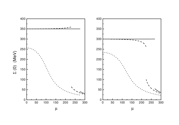
FIG. 1.: Behaviour of the self-energy as a function of the chemical potential for three representative values of the temperature. Full line corresponds to T=0, dashed line to $T=50$ MeV and dotted line to $T=100$ MeV. The left panels display the results for Set I and the right panels those for Set II.

We observe that at $T=0$ there is a first order phase transition for both the confining and the non-confining sets of parameters. As the temperature increases, the value of the chemical potential at which the transition shows up decreases. Finally, above a certain value of the temperature the first order phase transition does not longer exist and, instead, there is a smooth crossover. This phenomenon is clearly shown in the right panel of Fig. 2, where we display the critical temperature at which the phase transition occurs as a function of the chemical potential. The point at which the first order phase transition ceases to exist is usually called “end point”.

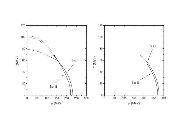
FIG. 2.: Critical temperatures as a function of the chemical potential. The left panel corresponds to the chiral limit and the right panel to the case of finite quark masses. In both panels the full line stands for a first order phase transition while in the left panel the dotted line indicates that the transition is of second order. The dashed line in the left panel indicates the temperature at which, for Set I, complex poles of the propagator turn into real poles.

In the chiral limit, the “end point” is expected to turn into a so-called “tricritical point”, where the second order phase transition expected to happen in QCD with two massless quarks becomes a first order one. Indeed, this is what happens within the present model for $m_{c}=0$, as it is shown in the left panel of Fig. 2. Some predictions about both the position of the “tricritical point” and its possible experimental signatures exist in the literature[12]. In our case this point is located at $(T_{P},\mu_{P})=$(70 MeV$,\,130$ MeV) for Set I and (70 MeV$,\,140$ MeV) for Set II, while the “end points” are placed at $(T_{E},\mu_{E})=$(70 MeV$,\,180$ MeV) and (55 MeV$,\,210$ MeV), respectively.

It is interesting to discuss in detail the situation concerning the confining set. In this case we can find, for each temperature, the chemical potential $\mu_{d}$ at which confinement is lost. Following the proposal of Ref.[9], this corresponds to the point at which the self-energy at zero momentum reaches the value $\Sigma(0)_{crit}$. Using the values of $m_{c}$ and $\Lambda$ corresponding to Set I we get $\Sigma(0)_{crit}=267$ MeV. For low temperatures, $\mu_{d}$ coincides with the the chemical potential at which the chiral phase transition takes place. However, for a temperature close enough to that of the “end point”, $\mu_{d}$ starts to be slightly smaller than the value of $\mu$ that corresponds to the chiral restoration. Above $T_{E}$ it is difficult to make an accurate comparison since, for finite quark masses, the chiral restoration proceeds through a smooth crossover. However, we can still study the situation in the chiral limit. In this case we find that, in the region where the chiral transition is of second order, deconfinement always occurs, for fixed $T$, at a lower value of $\mu$ than the chiral transition. The corresponding critical line is indicated by a dashed line in the left panel of Fig. 2. In any case, as we can see in this figure, the departure of the line of chiral restoration from that of deconfinement is in general not too large. This indicates that within the present model both transitions tend to happen at, approximately, the same point.

We turn now to the results for the instanton liquid model regulator. In this case we have

$$r(q^{2})=-z\,\frac{d}{dz}\left[I_{0}(z)K_{0}(z)-I_{1}(z)K_{1}(z)\right]$$ (11)

where $I$ and $K$ are the modified Bessel functions and

$$z=\frac{\sqrt{p^{2}}\ \rho}{2}$$ (12)

Here, $\rho$ stands for the instanton size. We take the standard value $\rho=1/3$ fm and fix the coupling constant to $G=36.7$ GeV^-2 so as to reproduce the typical value for the instanton density $n\approx 1$ fm^-4[5]. Using these values, together with $m_{c}=4.9$ MeV, it is possible to reproduce the empirical values of the pion mass and decay constant. The resulting value of the chiral quark condensate at zero temperature and chemical potential is $-(256$ MeV$)^{3}$. The behaviour of the quark self-energy as a function of the chemical potential is given in Fig. 3 for some representative values of the temperature.

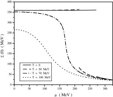
FIG. 3.: Quark self-energy in the instanton liquid model as a function of the chemical potential for some representative values of $T$.

As in the case of the gaussian regulator we observe that for low values of $T$ the chiral phase transition is of first order while for values above a certain $T_{E}$ the transition becomes a smooth crossover. The corresponding values of the critical temperature as a function of the chemical potential are displayed in Fig.4. The predicted position of the “end point” is in this case $(T_{E},\mu_{E})=$(65 MeV$,\,180$ MeV)

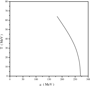
FIG. 4.: Critical temperatures as a function of the chemical potential in the instanton liquid model.

E Conclusions

In this work we investigate the features of the chiral phase transition in some non-local extensions of the NJL with covariant separable interactions. We consider two types of regulators: the Gaussian regulator and the instanton liquid model regulator. We find that in both cases the phase diagram is quite similar. In particular, we obtain that for two light flavors the transition is of first order at low values of the temperature and becomes a smooth crossover at a certain “end point”. Our predictions for the position of this point are very similar for both types of regulators and slightly smaller than the values in Refs.[12], $T_{P}~{}\approx~{}100$ MeV and $\mu_{P}\approx 200-230$ MeV. In this sense, we should remark that our model predicts a critical temperature at $\mu=0$ of about 100 MeV, somewhat below the values obtained in modern lattice simulations which suggest $T_{c}\approx 140-190$ MeV. In any case, our calculation seems to indicate that $\mu_{P}$ might be smaller than previously expected even in the absence of strangeness degrees of freedom.

Several extensions of this work are of great interest. For example, it would be very important to investigate the impact of the introduction of strangeness degrees of freedom and flavor mixing on the main features of the chiral phase transition. In addition, the competition between chiral symmetry breaking and color superconductivity at large chemical potential deserves further studies. Work along these lines is under way.

NNS would like to thank the organizers of the meeting “Dynamical aspects of the QCD phase transition” for their warm hospitality during his stay in Trento.

Equation of State for Strange Quark Matter in a Separable Model

Christian Gocke^†, David Blaschke^†,

Arman Khalatyan^‡, Hovik Grigorian^‡

^† Department of Physics, Rostock University, D-18051 Rostock, Germany
^‡ Department of Physics, Yerevan State University, 375 025 Yerevan, Armenia

A Introduction

Since the discovery of the parton substructure of nucleons and its interpretation within the constituent quark model, much effort has been spent to explain the properties of these particles. The phenomenon of confinement, i.e. the property of quarks to exist only in bound states as mesons and baryons in all known systems, poses great difficulties for a describing theory. So far the problem has been solved by introducing a color interaction that binds all colored particles to “colorless” states.

However, it is believed and new experimental results [1] underline it, that at very high temperatures exceeding $150$ MeV, or densities higher than three times nuclear matter density, a transition to deconfined quark matter can occur. Besides of the heavy ion collisions performed in particle physics, the existence of a deconfinement phase and its properties is of high importance for the understanding of compact stars [2] in astrophysics. These, that are popular as Neutron stars, imply core densities above three times the nuclear saturation density [3] so that quark matter is expected to occur in their interior and several suggestions have been made in order to detect signals of the deconfinement transition [4, 5].

Unfortunately, rigorous solutions of the fundamental theory of color interactions (Quantumchromodynamics (QCD)) for the EoS at finite baryon density could not be obtained yet, even Lattice gauge theory simulations have serious problems in this domain [6]. To describe interacting quark matter it is therefore necessary to find approximating models. The best studied one is the Nambu-Jona-Lasinio (NJL) model that was first developed to describe the interaction of nucleons [7] and has later been applied for modeling low-energy QCD [8, 9, 10] with particular emphasis on the dynamical breaking of chiral symmetry and the occurence of the pion as a quasi Goldstone boson. The application of the NJL model for studies of quark matter thermodynamics is problematic since it has no confinement and free quarks appear well below the chiral phase transition [11, 12]. This contradicts to results from lattice gauge theory simulations of QCD thermodynamics where the critical temperatures for deconfinement and chiral restoration coincide. That can be helped by using a separable model which can be treated similarly to the NJL model but includes a momentum dependence fo the interaction via formfactors. It has been shown [13] that in the chiral limit the model has no free quarks below the chiral transition.

Looking again at the densities of compact star cores and comparing with the results of NJL model calculations [12, 14] it seems reasonable to include strange-flavor quarks in the model because the energy density is sufficiently high for their creation in weak processes. Therefore, we extend in the present work the separable model to the case of three quark flavors, assuming for simplicity $U(3)$ symmetry. We will calculate the partition function using the method of bosonisation and applying the mean-field approximation. Finally we will formulate the resulting thermodynamics of three-flavor quark matter and obtain numerical results for the quark matter EoS and compact star structure.

B The separable quark model

The starting point of our approach is an effective chiral quark model action with a four-fermion interaction in the current-current form

$${\cal S}[q,\bar{q}] = \int\frac{d^{4}\!k}{(2\pi)^{4}}\big{[}\bar{q}(k)i(\!\not k+\hat{m})q(k)$$ (1)

$$+ D_{0}\int\frac{d^{4}\!k^{\prime}}{(2\pi)^{4}}\sum_{\alpha=0}^{8}[(\bar{q}(k)\lambda_{\alpha}f(k)q(k))(\bar{q}(k^{\prime})\lambda_{\alpha}f(k^{\prime})q(k^{\prime}))$$ (2)

$$+ (\bar{q}(k)i\gamma_{5}\lambda_{\alpha}f(k)q(k))(\bar{q}(k^{\prime})i\gamma_{5}\lambda_{\alpha}f(k^{\prime})q(k^{\prime}))]\big{]}~{}.$$ (3)

We restrict us here to the scalar and pseudoscalar currents in Dirac space which is invariant under chiral rotations of the quark fields and neglect color correlations (global color model). Furthermore we do not include one of the possible models to account for the $U_{A}(1)$ anomaly since, at least in the quark representation of the Di Vecchia - Veneziano model [15], it can be shown that there is no contribution to the quark thermodynamics on the mean-field level [16]. The generalization to the three-flavor case is done using the $U(3)$ symmetry where $\lambda_{\alpha}$ are the Gell-Mann matrices and $\lambda_{0}=\sqrt{\frac{2}{3}}I$. For the quark mass matrix in flavor space we use the notation

$$\hat{m}=\sum_{f}m_{f}P_{f}~{},$$ (4)

where $m_{f}$ are the current quark masses and the projectors $P_{f}$ on the flavor eigenstate $f=u,d,s$ are defined as

$$P_{u} = \frac{1}{\sqrt{6}}\lambda_{0}+\frac{1}{2}\lambda_{3}+\frac{1}{2\sqrt{3}}\lambda_{8},$$ (5)

$$P_{d} = \frac{1}{\sqrt{6}}\lambda_{0}-\frac{1}{2}\lambda_{3}+\frac{1}{2\sqrt{3}}\lambda_{8},$$ (6)

$$P_{s} = \frac{1}{\sqrt{6}}\lambda_{0}-\frac{1}{\sqrt{3}}\lambda_{8}~{}~{}.$$ (7)

Since the Matsubara frequencies in the $T\to 0$ limit become quasicontinuous variables, the summation over the fourth component $k_{4}$ of the 4-momentum has been replaced by the corresponding integration. According to the Matsubara formalism the calculations are performed in Euclidean space rather than in Minkowski space where we use $\gamma^{4}=i\gamma^{0}$. The partition function in Feynman’s path integral representation is given by

$${\cal Z}[T,\hat{\mu}]=\int{\cal D}\bar{q}{\cal D}q\exp\left({\cal S}[q,\bar{q}]-\int\frac{d^{4}\!k}{(2\pi)^{4}}i\hat{\mu}\gamma^{4}\bar{q}q\right)~{},$$ (8)

where the constraint of baryon number conservation is realized by the diagonal matrix of chemical potentials $\hat{\mu}$ (Lagrange multipliers) using the notation of the hat symbol analogous to (4).

In order to perform the functional integrations over the quark fields $\bar{q}$ and $q$ we use the formalism of bosonisation (see [17] and references therein) which is based on the Hubbard-Stratonovich transformation of the four-fermion interaction terms employing the identity

$$\exp\left\{D_{0}\int_{k}\int_{k^{\prime}}\sum_{\alpha=0}^{8}j_{s}^{\alpha}(k)j_{s}^{\alpha}(k^{\prime})\right\}=$$ (9)

$${\cal N}\prod_{\alpha}\int d\sigma^{\alpha}\exp\left[\frac{(\sigma^{\alpha})^{2}}{4D_{0}}+\int_{k}\int_{k^{\prime}}j_{s}^{\alpha}(k)\sigma^{\alpha}(k^{\prime})\right]~{},$$ (10)

for the scalar and a similar one for the pseudoscalar channel, where the abbreviations $\int_{k}=\int\frac{d^{4}\!k}{(2\pi)^{4}}$ for the phase space integral and $j_{s}^{\alpha}(k)=\bar{q}(k)\lambda_{\alpha}f(k)q(k)$ for the scalar current of the component $\alpha$ have been used. Now the generating functional is Gaussian with respect to the quark field and can be evaluated. We arrive at the transformed generating functional in terms of bosonic variables

$${\cal Z}[T,\hat{\mu}] = \int\!\!\!\int{\cal D}\sigma^{\alpha}{\cal D}\pi^{\alpha}\exp\left\{\cal{S}[\sigma^{\alpha},\pi^{\alpha}]\right\}$$ (11)

with the action functional

$${\cal S}[\sigma^{\alpha},\pi^{\alpha}]= - \int\frac{d^{4}\!k}{(2\pi)^{4}}\ln\left(\det_{DFC}[\not{\tilde{k}}+\hat{m}+\hat{\sigma}f(\tilde{k})+i\gamma_{5}\hat{\pi}f(\tilde{k})]\right)$$ (12)

$$+ \frac{\bar{\sigma}_{\alpha}\bar{\sigma}^{\alpha}}{4D_{0}}+\frac{\bar{\pi}_{\alpha}\bar{\pi}^{\alpha}}{4D_{0}}~{}.$$ (13)

with analogous use of the already known hat symbol and the 4-vector $\tilde{k}_{f}=\left({\vec{k}},{k_{4}+i\mu_{f}}\right)$. In order to further evaluate the integral over the auxiliary bosonic fields $\sigma_{\alpha}$ and $\pi_{\alpha}$ we expanded them around their mean values $\bar{\sigma}_{\alpha}$ and $\bar{\pi}_{\alpha}$ that minimize the action

$\displaystyle\begin{array}[]{r@{\:=\:}l}\sigma_{\alpha}\>=\>&\bar{\sigma}_{\alpha}+\tilde{\sigma}_{\alpha}(k)\\ \pi_{\alpha}\>=\>&\bar{\pi}_{\alpha}+\tilde{\pi}_{\alpha}(k)\end{array}$

and neglect the fluctuations $\tilde{\sigma}_{\alpha}(k)$ and $\tilde{\pi}_{\alpha}(k)$ in the following. The mean values of the pseudoscalar field vanish for symmetric reasons [16]. The indices $DFC$ refer to the determinant in Dirac-, flavor- and color- space. So we end up with the mean-field action

$${\cal S}_{\rm{MF}}[T,\{\mu_{f}\}] = \sum_{f}\left(-2N_{c}\int\frac{d^{4}\!k}{(2\pi)^{4}}[\ln(\tilde{k}_{f}^{2}+M_{f}^{2})]+\frac{\Delta_{f}^{2}}{8D_{0}}\right)~{},$$ (14)

with the effective quark masses $M_{f}=M_{f}(\tilde{k})=m_{f}+\Delta_{f}f(\tilde{k})$. The flavor dependent mass gaps $\Delta_{f}$ are defined by $\hat{\sigma}=\sum_{f}\Delta_{f}P_{f}$.

C Quark matter thermodynamics in mean field approximation

In the mean field approximation, the grand canonical thermodynamical potential is given by

$$\Omega(T,\{\mu\}) = \beta^{-1}\ln\left\{{\cal Z}[T,\{\mu_{f}\}]/{\cal Z}[0,\{0\}]\right\}$$ (15)

$$= \beta^{-1}\left\{{\cal S}_{\rm{MF}}[T,\{\mu_{f}\}]-{\cal S}_{\rm{MF}}[0,\{0\}]\right\}~{},$$ (16)

Where the divergent vacuum contribution has been subtracted. In what follows we consider the case $T=0$ only. In order to interpret our result, we want to represent it as a sum of three terms

$$\Omega(0,\{\mu\}) = \sum_{f}\left(-2N_{c}\int\frac{d^{4}\!k}{(2\pi)^{4}}\ln\left(\frac{\tilde{k}_{f}^{2}+M_{f}^{2}}{\tilde{k}_{f}^{2}+m_{f}^{2}}\right)+\frac{\Delta_{f}^{2}}{8D_{0}}\right)$$ (19)

$$-2N_{c}\sum_{f}\left(\int\frac{d^{4}\!k}{(2\pi)^{4}}\ln\left(\frac{\tilde{k}_{f}^{2}+m_{f}^{2}}{k_{f}^{2}+m_{f}^{2}}\right)\right)$$

$$+\sum_{f}\left(2N_{c}\int\frac{d^{4}\!k}{(2\pi)^{4}}\ln\left(\frac{k^{2}+(M_{f}^{0})^{2}}{k^{2}+m_{f}^{2}}\right)-\frac{(\Delta_{f}^{0})^{2}}{8D_{0}}\right)~{},$$

where $M_{f}^{0}=m_{f}+\Delta_{f}^{0}f(k^{2})$ are the effective quark masses in the vacuum. The second term on the r.h.s. of this equation is the renormalized thermodynamical potential of an ideal fermion gas [18]. The third term of Eq. (19) is independent of $T$ and $\mu$, i.e. it is a (thermodynamical) constant for the chosen model. Refering to the MIT bag model we call this term the bag-constant $B$. The remaining term includes the effects of quark interactions in the mean field approximation and can be evaluated numerically.

All thermodynamical quantities can now be derived from Eq. (19). For instance, pressure, density, energy density and the chiral condensate are given by:

$$pV=-\Omega\;,\;n=-\frac{\partial\Omega}{\partial\mu}\;,\;\varepsilon=-p+\mu n\;,\;<\!\bar{q}_{f}q_{f}\!>=\frac{\partial\Omega}{\partial m_{q}}~{}.$$ (20)

Still the quark mass gaps $\Delta_{f}$ have to be determined. This is done by solving the gap equations which follow from the minimization conditions $\frac{\partial\Omega}{\partial\Delta_{f}}=0$. The gap equations read

$$\Delta_{f}=4D_{0}(-2N_{c})\int\frac{d^{4}\!k}{(2\pi)^{4}}\frac{2M_{f}f(\tilde{k})}{\tilde{k}_{f}^{2}+M_{f}^{2}}~{}.$$ (21)

As can be seen from (21), for the chiral $U(3)$ quark model the three gap equations for $\Delta_{u},~{}\Delta_{d},~{}\Delta_{s}$ are decoupled and can be solved separately.

D Results for the Gaussian formfactor

1 Parametrization of the model

In the nonlocal separable quark model described above the formfactor of the interaction was not yet specified. In the following numerical investigations we will employ a simple Gaussian

$$f(k)=\exp(-k^{2}/\Lambda^{2})~{},$$ (22)

which has been used previously for the description of meson [19] and baryon [20] properties in the vacuum as well as for those of deconfinement and mesons at finite temperature [21, 22]. A systematic extension to other choices of formfactors is in preparation [23].

The Gaussian model has five free parameters to be defined: the coupling constant $D_{0}$, the interaction range $\Lambda$, and the three current quark masses $m_{u}$, $m_{d}$, $m_{s}$. Setting $m_{u}=m_{d}=:m_{q}$ we restrict ourselves to four free parameters. These are fixed by the three well known observables: pion mass $m_{\pi}=140$ MeV, kaon mass $m_{K}=494$ MeV and pion decay constant $f_{\pi}=93$ MeV. The formulas for the meson masses and the decay constant are calculated as approximations of the Bethe-Salpeter equation including the generalized Goldberger-Treiman relation [23].

The fourth condition comes from values for the chiral condensate that are conform with phenomenology. The resulting parametrisations of the quark model are shown in Tab. I.

$-<\!\bar{u}u+\bar{d}d\!>^{1/3}$	$\Lambda$	$D_{0}$	$m_{q}$	$m_{s}$	$\Delta_{q}^{0}$	$\Delta_{s}^{0}$
[MeV]	[MeV]	[GeV-2]	[MeV]	[MeV]	[MeV]	[MeV]
$230$	$659.2$	$29.32$	$6.8$	$143.5$	$549.9$	$767.8$
$235$	$697.6$	$23.88$	$6.4$	$136.1$	$497.0$	$719.3$
$240$	$736.5$	$19.88$	$6.0$	$129.5$	$453.8$	$682.1$
$245$	$775.5$	$16.85$	$5.6$	$123.4$	$419.7$	$653.1$
$250$	$814.9$	$14.49$	$5.3$	$118.0$	$391.1$	$630.0$
$255$	$853.8$	$12.66$	$5.0$	$112.9$	$368.7$	$611.4$
$260$	$894.2$	$11.11$	$4.7$	$108.1$	$349.1$	$596.1$

TABLE I.: Parameter sets for the Gaussian separable model for different values of the chiral condensate $<\!\bar{u}u+\bar{d}d\!>$.

2 Thermodynamics for quark matter without $\beta$ equilibrium

This case is relevant for systems which are considered for time scales larger than the typical strong interaction time of about $1$ fm/c but smaller than the weak interaction time of several minutes, so that the presence of leptons (electrons) does not influence on the composition of quark matter and we can choose the chemical equilibrium with $\mu_{u}=\mu_{d}=\mu_{s}=\mu$. For the numerical calculations we choose the parameter set for the light quark condensate $-\langle\bar{u}u+\bar{d}d\rangle^{1/3}=240$ MeV which is a typical value known from phenomenology. We consider the behavior of thermodynamical quantities at $T=0$ with respect to the chemical potential. As we set $m_{u}=m_{d}$ earlier there is no difference between up- and down quarks and both are refered to as light quarks. Fig. 1 visualizes the behavior of the thermodynamical potential as a function of the light quark gap $\Delta_{q}=\Delta_{u}=\Delta_{d}$ for different values of the chemical potential $\mu$. For $\mu<\mu_{c}=333$ MeV the argument and the value of the global minimum is independent of $\mu$ which corresponds to a vanishing quark density (confinement). At the critical value $\mu=\mu_{c}=333$ MeV a phase transition occurs from the massive, confining phase to a deconfining phase negligibly small mass gap. From the solution of the gap equation shown in Fig. 2

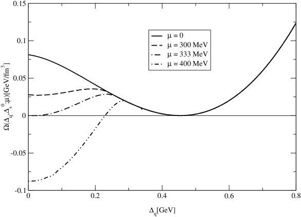
FIG. 1.: Dependence of the thermodynamical potential on the light flavor gap $\Delta_{q}=\Delta_{u}=\Delta_{d}$ (order parameter) for different values of the chemical potential, $\Delta_{s}=682$ MeV.

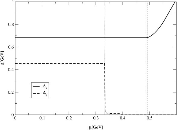
FIG. 2.: Solutions of the gap equations that minimize the potential

one can see that the strange quark gap of $\Delta_{s}=682$ MeV still remains unchanged. Thus the strange quarks are confined until a higher value of the chemical potential $\mu_{c,s}=492$ MeV is reached. This value is much bigger than the current strange quark mass. In Fig. 2 we separate by vertical lines the regions of full confinement, two-flavor deconfinement and full deconfinement. Thus, in the present model, the onset of strange quark deconfinement is inhibited. Moreover, the onset of a finite strange quark density is not determined by a drop in the strange gap which remains constant and even starts to rise for large $\mu$ values. This result of the present model drastically differs from those of bag models or NJL models. The reason is the 4-momentum dependence of the dynamical quark mass function which results in complex mass poles for the quark propagators and makes the naive identification of the mass gap with a real mass pole impossible [23].

The effect on thermodynamical quantities can be understood if we look at the pressure. In Fig. 3 we show for comparison the resulting equation of state for the pressure of the present separable model together with a two-flavor and a 3-flavor bag model. Both bag models are chosen such that the critical chemical potential for the deconfinement coincides with that of the separable model.

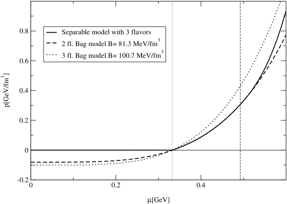
FIG. 3.: Pressure of the quark matter as a function of the chemical potential for the separable model (solid line) compared to a three-flavor (dotted line) and a two-flavor (dashed line) bag model. All models have the same critical chemical potential $\mu_{c}=333$ MeV for (light) quark deconfinement.

The pressure of the present three-flavor separable model can be well described by a two-flavor bag model with a bag constant $B=81.3$ MeV/fm³ in the region of chemical potentials $333$ MeV $\leq\mu\leq 492$ MeV where the third flavor is still confined. For comparison, the 3 flavor bag model has a the bag constant $B=100.7$ MeV/fm³ and is considerably harder that the separable one due to the additional relatively light strange quark flavor.

3 Inclusion of $\beta$ equilibrium with electrons

Quark matter in $\beta$-equilibrium is to be supplemented with the two relations for conservation of baryon charge and electric charge. In the deconfined phase there are quarks and leptons (in our model case up, down, strange quarks and electrons) with vanishing net electric charge

$$Q_{{\rm q}}(\mu^{u},\mu^{d},\mu^{s})+Q_{{\rm L}}(\mu^{e})={\frac{{2}}{{3}}}n_{u}-{\frac{{1}}{{3}}}(n_{d}+n_{s})-n_{e}=0~{}.$$ (23)

Taking into account the energy balance in weak interactions

$$d \leftrightarrow u+e^{-}+\bar{\nu}_{e}$$ (24)

$$s \leftrightarrow u+e^{-}+\bar{\nu}_{e}$$ (25)

and introducing the average quark chemical potential $\mu=\frac{1}{3}(\mu_{u}+\mu_{d}+\mu_{s})$ we can write the $\beta$ equilibrium conditions as

$$\mu_{u}=\mu-{\frac{{2}}{{3}}}\mu^{e}\,,\qquad\mu_{d}=\mu_{s}=\mu+{\frac{{1}}{{3}}}\,\mu^{e}\ .$$ (26)

Solving the equation of charge neutrality (23) one can find the chemical potential of electrons as a function of $\mu$ and using Eqs. (26) the equation of state can be given in terms of a single chemical potential $\mu$. In Fig. 4 we show the composition of the three-flavor quark matter for the Gaussian separable model in the case of $\beta$ equilibrium with electrons as a function of the energy density.

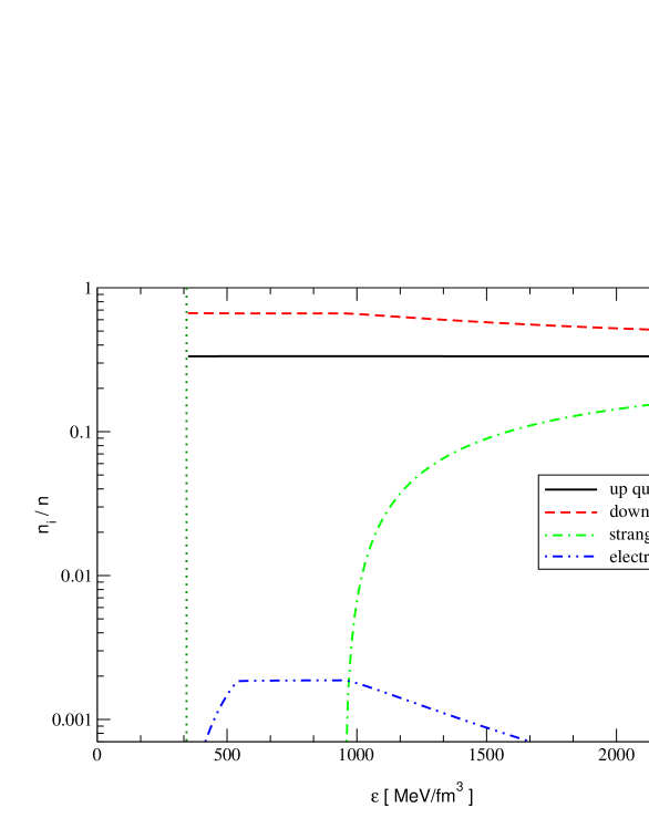
FIG. 4.: Composition of three-flavor quark matter in $\beta$ equilibrium with electrons.

As for the case without $\beta$ equilibrium we can define also in Fig. 4 the regions of quark confinement ($\varepsilon<\varepsilon_{c}=350$ MeV/fm³) and three-flavor deconfinement ($\varepsilon>\varepsilon_{c,s}=930$ MeV/fm³). In the region of two-flavor deconfinement the concentrations of electrons, up- and down- quarks coincide with those of the two-flavor bag model except for the relatively small energies close to $\varepsilon_{c}$ where the effect of a small dynamical quark mass leads to a density dependence of the composition. In Fig. 5 we demonstrate the influence of the $\beta$ equilibrium on the equation of state. It can be seen that the difference between pressures with and without $\beta$ equilibrium is limited to the region of intermediate densities, where the electron fraction reaches its maximum value $x_{e}\simeq 0.002$.

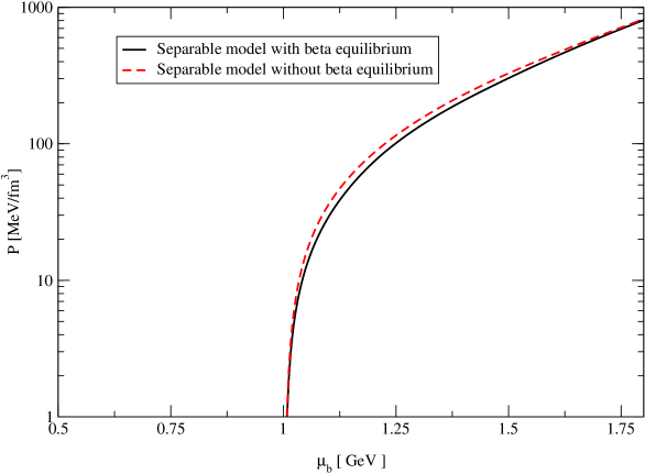
FIG. 5.: Pressure of three-flavor quark matter with $\beta$ equilibrium and without.

E Applications for compact stars

One of the main goals for studying the strange quark matter equation of state is the possible application for compact stars. In particular, the hypothesis that strange quark matter might be more stable than ordinary nuclear matter [24] has lead to the investigation of possible consequences for properties of compact stars made thereof [25]. Most of these applications use the bag model equation of state where the result depends on the value of the bag constant as a free parameter. Recently, first steps have been made towards a description of strange quark matter within dynamical quark models such as the NJL model [26], where the parameters are fixed from hadron properties. The non-confining quark dynamics of this model, however, leads to predictions for dynamical quark masses and critical parameters of the chiral phase transition which differ from those of confining models [27, 13] and might be quantitatively incorrect. Here we want to extend previous studies of compact star properties with dynamically confining quark models to the strange quark sector and find the characteristics of stable compact star configurations with the equation of state derived above.

For the calculation of the self-bound configuration for the quark matter with gravitational interaction one needs the condition of mechanical equilibrium of the thermodynamical pressure with the gravitational force. This condition is given by the Tolman-Oppenheimer-Volkoff-Equation

$$\frac{dP}{dr}=-G(\varepsilon(r)+P(r))\frac{m(r)+4\pi Gr^{3}P(r)}{r(r-2Gm(r))}~{}$$ (27)

and defines the profiles for all thermodynamical quantities in the case of nonrotating spherically symmetric distributed matter configurations in general relativity. In this equation $m$ denotes the accumulated mass in the sphere with radius $r$ given by

$$m(r)=4\pi\int_{0}^{r}\varepsilon(r^{\prime})r^{\prime 2}dr$$ (28)

The gravitational constant is denoted by $G$. The radius $R$ of the star is defined by the condition that the pressure becomes zero on the surface of the star $P(R)=0$. The total mass of the star is $M=m(R)$.

Each configuration has one independent parameter which could be chosen to be $\varepsilon(0)$, the central energy density. In Fig. 6 we show the dependence of the total mass of the configuration as a function of the central density and the radius for the separable quark model and for the bag model in the cases of two and three flavors respectively.

The rising branches of the mass-radius or mass-density relations correspond to the families of stable compact stars. The maximum possible mass for the separable model is $1.64~{}M_{\odot}$ for the three-flavor and $1.71~{}M_{\odot}$ for the two-flavor case. The maximal central density is about $1350$ MeV/fm³ which allows for the three-flavor case to have strange quark matter in the core of the quark star. The comparison with the corresponding bag model strange stars shows that the latter are more compact, their maximum radius is about $8$ km, and less massive with a maximum mass of about $1.5~{}M_{\odot}$. The maximum radius of stars within the separable model is 11 km and thus exceeds the radii for both two and three flavor bag model quark stars. The origin of this difference is the behavior of the pressure in the low density region.

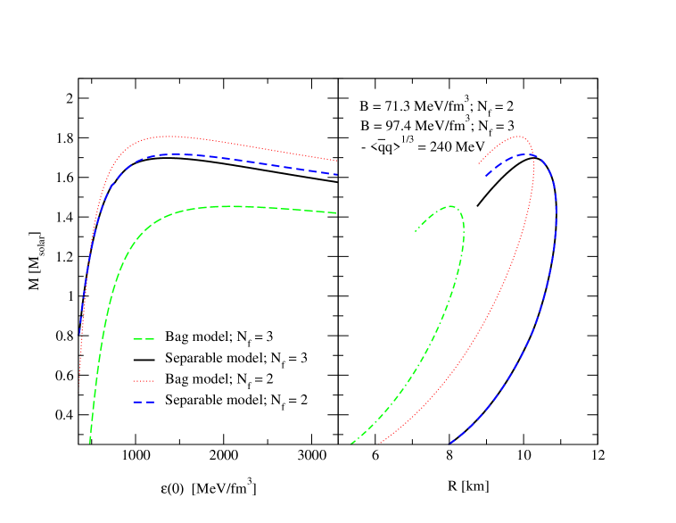
FIG. 6.: Stability for compact stars composed of quark matter.

F Conclusion

For neutron stars it is relevant to include the effects of strange flavor in a model for quark matter. In the simplest case considering $U(3)$ symmetry this can be done without increasing the complexity of the generating functional. We showed that in our separable model the gap equations decouple and can be solved separately. The resulting thermodynamics can be solved numerically and gives the equations of state for interacting quark matter. Unlike the well known NJL model the separable model is able to express the effects of confinement in the thermodynamical quantities. The new result obtained within the present approach is the separation of the deconfinement of light quark flavors at $\mu_{c}=333$ MeV from that of strange quarks which occurs only at a higher chemical potential of $\mu_{c,s}=502$ MeV. A consequence for the application of the EoS presented here in compact star calculations is that strange quarks do occur only close to the maximum mass of $1.64~{}M_{\odot}$, i.e. that for masses below $1.62~{}M_{\odot}$, only two-flavor quark matter can occur.

Acknowledgments

We like to thank our colleagues M. Buballa, Y. Kalinovsky, M. Ruivo, N. Scoccola and P.C. Tandy. Their studies of separable quark models have helped us to formulate the present one. We are grateful to R. Alkofer for pointing out Ref. [16] to us. We acknowledge the support of DAAD and DFG for scientist exchange between the Universities of Rostock and Yerevan.

Quark Matter Effects in the Cooling and Spin Evolution of Neutron Stars

David Blaschke^†, Gevorg Poghosyan^†,

Hovik Grigorian^‡

^† Department of Physics, University of Rostock, D-18051 Rostock, Germany
^‡ Department of Physics, Yerevan State University, Alex Manoogian 1,
375025 Yerevan, Armenia

A Introduction

Quantum Chromodynamics (QCD) as the fundamental theory for strongly interacting matter predicts a deconfined state of quarks and gluons under conditions of sufficiently high temperatures and/or densities which occur, e.g., in heavy-ion collisions, a few microseconds after the Big Bang or in the cores of pulsars. The unambiguous detection of the phase transition from hadronic to quark matter (or vice-versa) has been a challenge to particle and astrophysics over the past two decades [1, 2]. While the diagnostics of a phase transition in experiments with heavy-ion beams faces the problems of strong nonequilibrium and finite size, the dense matter in a compact star forms a macroscopic system in thermal and chemical equilibrium for which signals of a phase transition shall be more pronounced. Particularly interesting systems for investigating the possible occurence of quark matter in neutron star interiors are accreting compact stars in low-mass X-ray binaries. Due to their mass accretion flow these systems are candidates for the most massive compact stars in nature at the limit of black hole formation. Therefore, if the possible deconfinement phase transition in compact stars exists at all, we expect it to occur in these systems. Typical time scales for the deconfinement transition due to either the accretion of a fraction of the solar mass or due to frequency changes by a fraction of a kHz are larger than $10^{8}$ yr.

These timescales for rotational evolution seem well separated from those of thermal processes which leave traces from the composition of the neutron star interior during the time which a heat wave travels from the center to the surface of the star, i.e. less than $10^{3}$ yr.

A completely new situation might arise if the scenarios suggested for (color) superconductivity [3, 4] with large diquark pairing gaps ($\Delta_{q}\sim 50\div 100$ MeV) in quark matter are applicable to neutron star interiors. Then, fast temperature drops could occur between $10\div 500$ yr after the birth of the compact star depending on the size of the pairing gaps. The diquark pairing changes the specific heat of quark matter and therefore a different photon cooling asymptotics results in the case of color superconductivity. Unfortunately, the photon cooling era (after $10^{6}\div 10^{8}$ yr) does not allow to distinguish between details of the internal structure such as sizes of gaps and of the quark core.

The question arises whether there are candidates of compact objects which are young enough to reveal their internal composition by their cooling behaviour and which could traverse the critical phase transition line within less than $100$ yr. For the latter condition to be fulfilled, these objects should rotate fast enough (period $P\sim 2$ ms) and the braking torque acting on them should be large enough to make their spindown age small enough.

It is interesting to note the recently reported $2.14$ ms optical pulsar candidate in SN 1987A [5] would fulfill these requirements and it could be interesting to investigate the combined effects of deconfinement on rotational and cooling evolution more in detail and develop speculations about the mysterious disappearance of this source $6.5$ yr after the supernova explosion.

In this contribution we will review the status of the separate investigations of quark matter effects in the cooling and rotational evolution of neutron stars.

B Cooling of young neutron stars

Let us consider how the color superconducting quark matter, if it exists in interiors of massive neutron stars, may affect the neutrino cooling of hybrid neutron stars (HNS), see [6]. Various phases are possible. The two-flavor (2SC) or the three-flavor (3SC) superconducting phases allow for unpaired quarks of one color whereas in the color-flavor locking (CFL) phase all the quarks are paired.

Estimates of the cooling evolution have been performed [7] for a self-bound isothermal quark core neutron star (QCS) which has a crust but no hadron shell, and for a quark star (QS) which has neither crust nor hadron shell. It has been shown there in the case of the 2SC (3SC) phase of a QCS that the consequences of the occurrence of gaps for the cooling curves are similar to the case of usual hadronic neutron stars (enhanced cooling). However, for the CFL case it has been shown that the cooling is extremely fast since the drop in the specific heat of superconducting quark matter dominates over the reduction of the neutrino emissivity. As has been pointed out there, the abnormal rate of the temperature drop is the consequence of the approximation of homogeneous temperature profiles the applicability of which should be limited by the heat transport effects. Page et al. (2000) estimated the cooling of HNS where heat transport effects within the superconducting quark core have been disregarded. Neutrino mean free paths in color superconducting quark matter have been discussed in [8] where a short period of cooling delay at the onset of color superconductivity for a QS has been conjectured in accordance with the estimates of [7] in the CFL case for small gaps.

A detailed discussion of the neutrino emissivity of quark matter without taking into account of the possibility of the color superconductivity has been given first in Ref. [9]. In this work the quark direct Urca (QDU) reactions $d\rightarrow ue\bar{\nu}$ and $ue\rightarrow d{\nu}$ have been suggested as the most efficient processes. In the color superconducting matter the corresponding expression for the emissivity modifies as

$\displaystyle\epsilon_{\nu}^{{\rm QDU}}\simeq 9.4\times 10^{26}\alpha_{s}(\varrho/\varrho_{0})Y_{e}^{1/3}\zeta_{{\rm QDU}}~{}T_{9}^{6}~{}{\rm erg~{}cm^{-3}~{}s^{-1}},$

where due to the pairing the emissivity of QDU processes is suppressed by a factor, very roughly given by $\zeta_{{\rm QDU}}\sim\mbox{exp}(-\Delta_{q}/T)$. At $\varrho/\varrho_{0}\simeq 2$ the strong coupling constant is $\alpha_{s}\approx 1$ decreasing logarithmically at still higher densities, $Y_{e}=\varrho_{e}/\varrho$ is the electron fraction. If for somewhat larger density the electron fraction was too small ($Y_{e}<Y_{ec}\simeq 10^{-8}$), then all the QDU processes would be completely switched off [10] and the neutrino emission would be governed by two-quark reactions like the quark modified Urca (QMU) and the quark bremsstrahlung (QB) processes $dq\rightarrow uqe\bar{\nu}$ and $q_{1}q_{2}\rightarrow q_{1}q_{2}\nu\bar{\nu}$, respectively. The emissivities of QMU and QB processes are smaller than that for QDU being suppressed by factor $\zeta_{{\rm QMU}}\sim\mbox{exp}(-2\Delta_{q}/T)$ for $T<T_{{\rm crit},q}\simeq 0.4~{}\Delta_{q}$. For $T>T_{{\rm crit},q}$ all the $\zeta$ factors are equal to unity. The modification of $T_{{\rm crit},q}(\Delta_{q})$ relative to the standard BCS formula is due to the formation of correlations as, e.g., instanton- anti-instanton molecules. The contribution of the reaction $ee\rightarrow ee\nu\bar{\nu}$ to the emissivity is very small [11], $\epsilon_{\nu}^{ee}\sim 10^{12}\,Y_{e}^{1/3}(\varrho/\varrho_{0})^{1/3}T_{9}^{8}~{}{\rm erg~{}cm^{-3}~{}s^{-1}}$, but it can become important when quark processes are blocked out for large values of $\Delta_{q}/T$ in superconducting quark matter.

For the quark specific heat [6] used expression of [9] being however suppressed by the corresponding $\zeta$ factor due to color superfluidity. Therefore gluon-photon and electron contributions play important role.

The heat conductivity of the matter is the sum of partial contributions $\kappa=\sum_{i}\kappa_{i},\,\,\,\kappa_{i}^{-1}=\sum_{j}\kappa_{ij}^{-1}~{},$ where $i,j$ denote the components (particle species). For quark matter $\kappa$ is the sum of the partial conductivities of the electron, quark and gluon components $\kappa=\kappa_{e}+\kappa_{q}+\kappa_{g}$, where $\kappa_{e}\simeq\kappa_{ee}$ is determined by electron-electron scattering processes since in superconducting quark matter the partial contribution $1/\kappa_{eq}$ (as well as $1/\kappa_{gq}$ ) is additionally suppressed by a $\zeta_{{\rm QDU}}$ factor, as for the scattering on impurities in metallic superconductors. Due to very small resulting value of $\kappa$ the typical time necessary for the heat to reach the star surface is large, delaying the cooling of HNS.

The equation of state (EoS) used in Ref. [6] included a model for hadronic matter, and regions of mixed phase and of pure quark matter. A hard EoS for the hadron matter was used, finite size effects were disregarded in description of the mixed phase, and the bag constant $B$ was taken to be rather small as motivated from confining chiral quark models [12, 13]. That led to the presence of a wide region of mixed and quark phases already for the HNS of the mass $M=1.4~{}M_{\odot}$. On the other hand, the absence of a dense hadronic region within this EoS allowed to diminish uncertainties in the description of in-medium effects in hadronic matter suppressing them relative to that used in the ”standard scenario”.

With the above inputs, the evolution equation for the temperature profile has been solved in Ref. [6]. In order to demonstrate the influence of the size of the diquark and nucleon pairing gaps on the evolution of the temperature profile solutions were performed with different values of the quark and nucleon gaps. Comparison of the cooling evolution ($\mbox{lg}~{}T_{s}$ vs. $\mbox{lg}~{}t$) of HNS of the mass $M=1.4~{}M_{\odot}$ is given in Fig. 1. The curves for $\Delta_{q}\stackrel{{\scriptstyle\scriptstyle>}}{{\phantom{}{}_{\sim}}}1$ MeV are very close to each other demonstrating typical large gap behaviour. The behaviour of the cooling curve for $t\leq 50\div 100$ yr is in straight correspondence with the heat transport processes. The subsequent time evolution is governed by the processes in the hadronic shell and by a delayed transport within the quark core with a dramatically suppressed neutrino emissivity from the color superconducting region. In order to demonstrate this feature a calculation was performed with the nucleon gaps ($\Delta_{i}(n),~{}i=n,p$) being artificially suppressed by a factor 0.2. Then up to $\mbox{lg}(t[{\rm yr}])\stackrel{{\scriptstyle\scriptstyle<}}{{\phantom{}{}_{\sim}}}4$ the behaviour of the cooling curve is analogous to the one would be obtained for pure hadronic matter. The curves labelled ”MMU” show the cooling of hadron matter with inclusion of appropriate medium modifications in the $NN$ interaction.

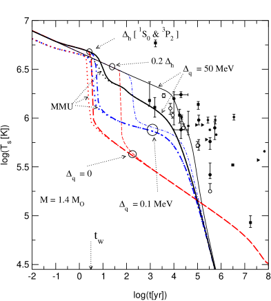
FIG. 1.: Evolution of the surface temperature $T_{s}$ of HNS with $M=1.4M_{\odot}$ for $T_{s}=(10T_{m})^{2/3}$, where $T$ is in K, see [14]. Data are from [15] (full symbols) and from [16] (empty symbols), $t_{w}$ is the typical time which is necessary for the cooling wave to pass through the crust.

These effects have an influence on the cooling evolution only for $\mbox{lg}(t[{\rm yr}])\stackrel{{\scriptstyle\scriptstyle<}}{{\phantom{}{}_{\sim}}}2$ since the specific model EQS used does not allow for high nucleon densities in the hadron phase at given example of HNS of $M=1.4~{}M_{\odot}$. The effect would be much more pronounced for larger star masses, a softer EQS for hadron matter and smaller values of the gaps in the hadronic phase. Besides, incorporation of finite size effects within description of the mixed phase reducing its region should enlarge the size of the pure hadron phase.

The unique asymptotic behaviour at $\mbox{lg}(t[{\rm yr}])\geq 5$ for all the curves corresponding to finite values of the quark and nucleon gaps is due to a competition between normal electron contribution to the specific heat and the photon emissivity from the surface since small exponentials switch off all the processes related to paired particles. This tail is very sensitive to the interpolation law $T_{s}=f(T_{m})$ used to simplify the consideration of the crust. The curves coincide at large times due to the uniquely chosen relation $T_{s}\propto T_{m}^{2/3}$.

The curves for $\Delta_{q}=0.1$ MeV demonstrate an intermediate cooling behaviour between those for $\Delta_{q}=50$ MeV and $\Delta_{q}=0$. Heat transport becomes not efficient after first $5\div 10$ yr. The subsequent $10^{4}$ yr evolution is governed by QDU processes and quark specific heat being only moderately suppressed by the gaps and by the rates of NPBF processes in the hadronic matter (up to $\mbox{lg}(t[{\rm yr}])\leq 2.5$). At $\mbox{lg}(t[{\rm yr}])\geq 4$ begins the photon cooling era.

The curves for normal quark matter ($\Delta_{q}=0$) are governed by the heat transport at times $t\stackrel{{\scriptstyle\scriptstyle<}}{{\phantom{}{}_{\sim}}}5$ yr and then by QDU processes and the quark specific heat. The NPBF processes are important up to $\mbox{lg}(t[{\rm yr}])\leq 2$, the photon era is delayed up to $\mbox{lg}(t[{\rm yr}])\geq 7$. For times smaller than $t_{w}$ (see Fig. 1) the heat transport is delayed within the crust area [17]. Since for simplicity this delay was disregarded in the heat transport treatment, for such small times the curves should be interpreted as the $T_{m}(t)$ dependence scaled to guide the eye by the same law $\propto T_{m}^{2/3}$, as $T_{s}$.

For the CFL phase with large quark gap, which is expected to exhibit the most prominent manifestations of color superconductivity in HNS and QCS configurations, [6] thus demonstrated an essential delay of the cooling during the first $50\div 300$ yr (the latter for a QCS) due to a dramatic suppression of the heat conductivity in the quark matter region. This delay makes the cooling of HNS and QCS systems not as rapid as one could expect when ignoring the heat transport. In HNSs compared to QCSs (large gaps) there is an additional delay of the subsequent cooling evolution which comes from the processes in pure hadronic matter.

In spite of that we find still too fast cooling for those objects compared to ordinary NS. Therefore, with the CFL phase of large quark gap it seems rather difficult to explain the majority of the presently known data both in the cases of the HNS and QCS, whereas in the case of pure hadronic stars the available data are much better fitted even within the same simplified model for the hadronic matter. For 2SC (3SC) phases one may expect analogous behaviour to that demonstrated by $\Delta_{q}=0$ since QDU processes on unpaired quarks are then allowed, resulting in a fast cooling. It is however not excluded that new observations may lead to lower surface temperatures for some supernova remnants and will be better consistent with the model which also needs further improvements. On the other hand, if future observations will show very large temperatures for young compact stars they could be interpreted as a manifestation of large gap color superconductivity in the interiors of these objects.

C Spin evolution of old neutron stars

It is the aim of the present paper to investigate the conditions for an observational verification of the existence of the critical line $N_{{\rm crit}}(\Omega)$ which separates the QCS configurations from hadronic ones. We will show evidence that in principle such a measurement is possible since this deconfinement transition line corresponds to a maximum of the moment of inertia, which is the key quantity for the rotational behavior of compact objects, see Fig. 2.

In the case of rigid rotation the moment of inertia is defined by

$$I(\Omega,N)=J(\Omega,N)/\Omega~{},$$ (1)

where the angular momentum $J(\Omega,N)$ of the star can be expressed in invariant form as

$$J(\Omega,N)=\int T_{\phi}^{t}\sqrt{-g}dV~{},$$ (2)

with $T_{\phi}^{t}$ being the nondiagonal element of the energy momentum tensor, $\sqrt{-g}dV$ the invariant volume and $g=\det||g_{\mu\nu}||$ the determinant of the metric tensor. We assume that the superdense compact object rotates stationary as a rigid body, so that for a given time-interval both the angular velocity as well as the baryon number can be considered as global parameters of the theory. The result of our calculations for the moment of inertia (1) can be cast into the form

$$I=I^{(0)}+\sum_{\alpha}\Delta I_{\alpha},$$ (3)

where $I^{(0)}$ is the moment of inertia of the static configuration with the same central density and $\Delta I_{\alpha}$ stands for contributions to the moment of inertia from different rotational effects which are labeled by $\alpha$: matter redistribution, shape deformation, and changes in the centrifugal forces and the gravitational field [18].

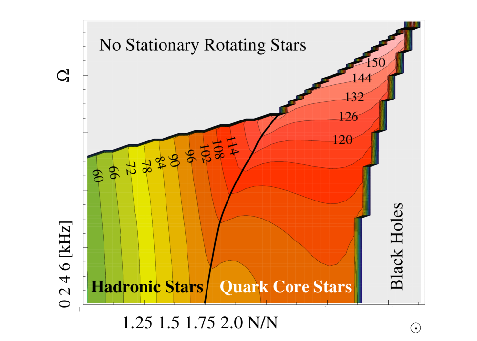
FIG. 2.: Phase diagram for configurations of rotating compact objects in the plane of angular velocity $\Omega$ and mass (baryon number $N$). Contour lines show the values of the moment of inertia in M_⊙km². The line $N_{{\rm crit}}(\Omega)$ which separates hadronic from quark core stars corresponds the set of configurations with a central density equal to the critical density for the occurence of a pure quark matter phase..

In Fig. 2 we show the resulting phase diagram for compact star configurations which exhibits four regions: (i) the region above the maximum frequency $\Omega_{{\rm K}}(N)$ where no stationary rotating configurations are found, (ii) the region of black holes for baryon numbers exceeding the maximum value $N_{{\rm max}}(\Omega)$, and the region of stable compact stars which is subdivided by the critical line $N_{{\rm crit}}(\Omega)$ into a region of (iii) quark core stars and another one of (iv) hadronic stars, respectively. The numerical values for the critical lines are model dependent. For this particular model EoS due to the hardness of the hadronic branch (linear Walecka model [19]) there is a maximum value of the baryonic mass on the critical line $N_{{\rm crit}}(\Omega_{k})=1.8N_{\odot}$, such that for stars more massive than that one all stable rotating configurations have to have a quark core.

The simple case of the spindown evolution of isolated (non-accreting) pulsars due to magnetic dipole radiation would be described by vertical lines in Fig. 2. All other possible trajectories correspond to processes with variable baryon number (accretion). In the phase of hadronic stars, $\dot{\Omega}$ first decreases as long as the moment of inertia monotonously increases with $N$. When passing the critical line $N_{{\rm crit}}(\Omega)$ for the deconfinement transition, the moment of inertia starts decreasing and the internal torque term $K_{{\rm int}}$ changes sign. This leads to a narrow dip for $\dot{\Omega}(N)$ in the vicinity of this line. As a result, the phase diagram gets populated for $N\stackrel{{\scriptstyle<}}{{\sim}}N_{{\rm crit}}(\Omega)$ and depopulated for $N\stackrel{{\scriptstyle>}}{{\sim}}N_{{\rm crit}}(\Omega)$ up to the second maximum of $I(N,\Omega)$ close to the black-hole line $N_{{\rm max}}(\Omega)$. The resulting population clustering of compact stars at the deconfinement transition line is suggested to emerge as a signal for the occurence of stars with quark matter cores. In contrast to this scenario, in the case without a deconfinement transition, the moment of inertia could at best saturate before the transition to the black hole region and consequently $\dot{\Omega}$ would also saturate. This would entail a smooth population of the phase diagram without a pronounced structure.

The clearest scenario could be the evolution along lines of constant $\Omega$ in the phase diagram. These trajectories are associated with processes where the external and internal torques are balanced. A situation like this has been described, e.g. by [20] for accreting binaries emitting gravitational waves.

We consider the spin evolution of a compact star under mass accretion from a low-mass companion star as a sequence of stationary states of configurations (points) in the phase diagram spanned by $\Omega$ and $N$. The process is governed by the change in angular momentum of the star

$$\frac{d}{dt}(I(N,\Omega)~{}\Omega)=K_{{\rm ext}}~{},$$ (4)

where

$$K_{{\rm ext}}=\sqrt{GM\dot{M}^{2}r_{0}}-N_{{\rm out}}$$ (5)

is the external torque due to both the specific angular momentum transfered by the accreting plasma and the magnetic plus viscous stress given by $N_{{\rm out}}=\kappa\mu^{2}r_{c}^{-3}$, $\kappa=1/3$ [21]. For a star with radius $R$ and magnetic field strength $B$, the magnetic moment is given by $\mu=R^{3}~{}B$. The co-rotating radius $r_{c}=\left(GM/\Omega^{2}\right)^{1/3}$ is very large ($r_{c}\gg r_{0}$) for slow rotators. The inner radius of the accretion disc is

$\displaystyle r_{0}\approx\left\{\begin{array}[]{cc}R~{},&\mu<\mu_{c}\\ 0.52~{}r_{A}~{},&\mu\geq\mu_{c}\end{array}\right.$

where $\mu_{c}$ is that value of the magnetic moment of the star for which the disc would touch the star surface. The characteristic Alfvén radius for spherical accretion with the rate $\dot{M}=m\dot{N}$ is $r_{A}=\left(2\mu^{-4}GM\dot{M}^{2}\right)^{-1/7}$. Since we are interested in the case of fast rotation for which the spin-up torque due to the accreting plasma in Eq. (5) is partly compensated by $N_{{\rm out}}$, eventually leading to a saturation of the spin-up, we neglect the spin-up torque in $N_{{\rm out}}$ which can be important only for slow rotators [22],

From Eqs. (4), (5) one can obtain the first order differential equation for the evolution of angular velocity

$$\frac{d\Omega}{dt}=\frac{K_{{\rm ext}}(N,\Omega)-K_{{\rm int}}(N,\Omega)}{I(N,\Omega)+{\Omega}({\partial I(N,\Omega)}/{\partial\Omega})_{N}}~{},$$ (6)

where

$$K_{{\rm int}}(N,\Omega)=\Omega\dot{N}({\partial I(N,\Omega)}/{\partial N})_{\Omega}~{}.$$ (7)

Solutions of (6) are trajectories in the $\Omega-N$ plane describing the spin evolution of accreting compact stars. Since $I(N,\Omega)$ exhibits characteristic functional dependences [23] at the deconfinement phase transition line $N_{{\rm crit}}(\Omega)$ we expect observable consequences in the $\dot{P}-P$ plane when this line is crossed.

In our model calculations we assume that both the mass accretion and the angular momentum transfer processes are slow enough to justify the assumption of quasistationary rigid rotation without convection. The moment of inertia of the rotating star can be defined as $I(N,\Omega)=J(N,\Omega)/\Omega~{}$, where $J(N,\Omega)$ is the angular momentum of the star. For a more detailed description of the method and analytic results we refer to [18] and the works of [24, 25], as well as [26, 27].

The time dependence of the baryon number for the constant accreting rate $\dot{N}$ is given by

$$N(t)=N(t_{0})+(t-t_{0})\dot{N}~{}.$$ (8)

For the magnetic field of the accretors we consider the exponential decay [28]

$$B(t)=[B(0)-B_{\infty}]\exp(-t/\tau_{B})+B_{\infty}~{}.$$ (9)

We solve the equation for the spin-up evolution (6) of the accreting star for decay times $10^{7}\leq\tau_{B}{\rm[yr]}\leq 10^{9}$ and initial magnetic fields in the range $0.2\leq B(0){\rm[TG]}\leq 4.0$. The remnant magnetic field is chosen to be $B_{\infty}=10^{-4}$TG [29].

At high rotation frequency, both the angular momentum transfer from accreting matter and the influence of magnetic fields can be small enough to let the evolution of angular velocity be determined by the dependence of the moment of inertia on the baryon number, i.e. on the total mass. This case is similar to the one with negligible magnetic field considered in [18, 30, 31] where $\mu\leq\mu_{c}$ in Eq. (6), so that only the so called internal torque term (7) remains.

1 Waiting time and population clustering

The question arises whether there is any characteristic feature in the spin evolution which distinguishes trajectories that traverse the critical phase transition line from those remaining within the initial phase.

The results of Ref. [32] show that the waiting time for accreting stars along their evolution trajectory is larger in a hadronic configuration than in a QCS, after a time scale when the mass load onto the star becomes significant. This suggests that if a hadronic star enters the QCS region, its spin evolution gets enhanced thus depopulating the higher frequency branch of its trajectory in the $\Omega-N$ plane. In Fig. 3 we show contours of waiting time regions in the phase diagram. The initial baryon number is $N(0)=1.4N_{\odot}$ and the initial magnetic field is taken from the interval $0.2\leq B(0)[{\rm TG}]\leq 4.0$ .

The region of longest waiting times is located in a narrow branch around the phase transition border and does not depend on the evolution scenario after the passage of the border, when the depopulation occurs and the probability to find an accreting compact star is reduced. Another smaller increase of the waiting time and thus a population clustering could occur in a region where the accretor is already a QCS. For an estimate of a population statistics we show the region of evolutionary tracks when the values of initial magnetic field are within $0.6\leq B(0)[{\rm TG}]\leq 1.0$ as suggested by the observation of frequency clustering in the narrow interval $375\geq\nu[{\rm Hz}]\geq 225$.

As a strategy of search for QCSs we suggest to select from the LMXBs exhibiting the QPO phenomenon those accreting close to the Eddington limit [28] and to determine simultaneously the spin frequency and the mass [33] for sufficiently many of these objects. The emerging statistics of accreting compact stars should then exhibit the population clustering shown in Fig. 3 when a deconfinement transition is possible. If a structureless distribution of objects in the $\Omega-N$ plane will be observed, then no firm conclusion about quark core formation in compact stars can be made.

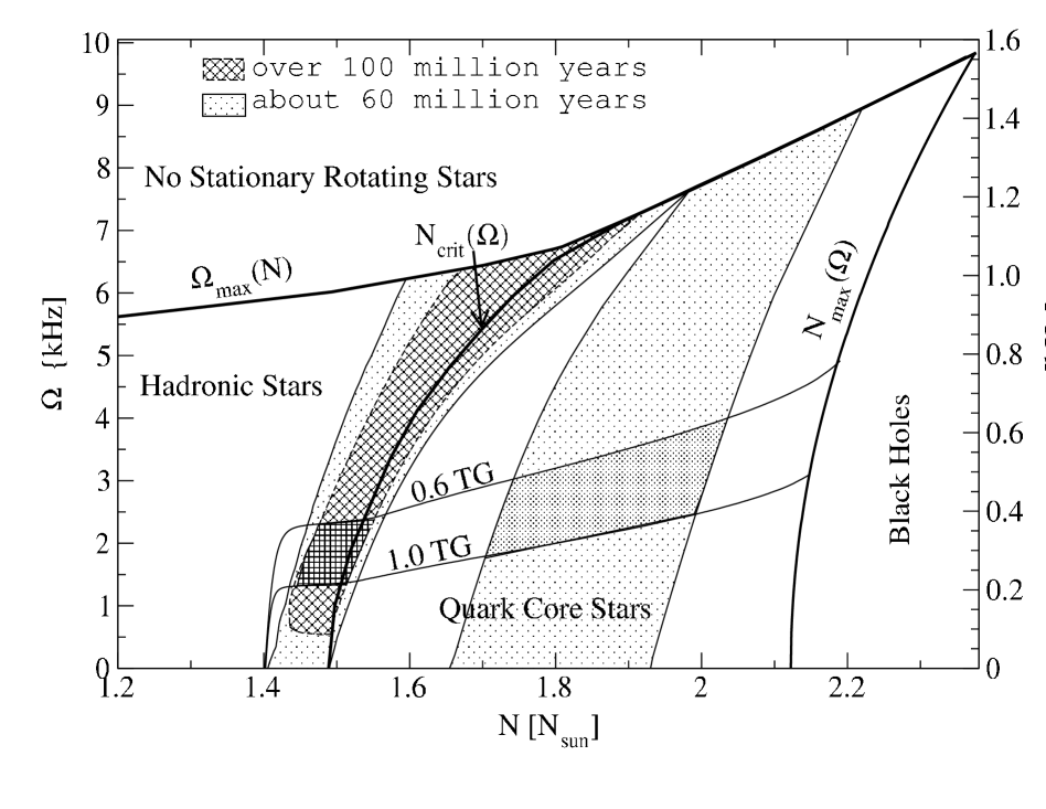
FIG. 3.: Regions of waiting times in the phase diagram for compact hybrid stars for the (9,-8) scenario. For an estimate of a population statistics we show the region of evolutionary tracks when the interval of initial magnetic field values is restricted to $0.6\leq B(0)[{\rm TG}]\leq 1.0$. Note that the probability of finding a compact star in the phase diagram is enhanced in the vicinity of the critical line for the deconfinement phase transition $N_{{\rm crit}}(\Omega)$ by at least a factor of two relative to all other regions in the phase diagram.

For the model equation of state on which the results of our present work are based, we expect a baryon number clustering rather than a frequency clustering to be a signal of the deconfinement transition in the compact stars of LMXBs. The model independent result of our study is that a population clustering in the phase diagram for accreting compact stars shall measure the critical line $N_{{\rm crit}}(\Omega)$ which separates hadronic stars from QCSs where the shape of this curve can discriminate between different models of the nuclear EoS at high densities.

D Conclusion

The investigations of cooling and rotational evolution of compact stars with quark matter cores show that the presence of quark matter in these objects could be an observable phenomenon. In order to develop the prognosis of signals for the occurence of quark matter in neutron stars further, and to identify candidate objects for this phenomenon, we need to improve the scenarios presented here in several ways.

On the one hand the models for the EoS need to be improved so that one goes beyond the simple mean-field level of description. The equation of state could be further constrained not only by the saturation properties of nuclear matter but also by comparison with informations about excitation properties and softness obtained from relativistic heavy-ion collisions.

On the other hand the scenarii for quark matter occurence should be developed. It is conceivable that already in the hot and dense protoneutron star stage immediately after a supernova explosion quark matter can occur and modify the propagation of neutrinos [34]. Effects on the hydrodynamical, gravitational and cooling evolution are expected.

A particularly interesting aspect is the possibility of cross-effects between: rotation and cooling (see introduction), accretion and cooling, magnetic field and rotation, etc. which leads to the prediction of correlations between observables. Such stronger constraints will help to prove or disprove the hypothesis of quark matter occurence in neutron stars.

Acknowledgement

The results for the cooling evolution of neutron stars reported here are based on an approach which has been developed together with D.N. Voskresensky. This work is a result of the collaboration between the Universities of Rostock and Yerevan which is supported by a DAAD program. G.P. acknowledges support by DFG under grant No. ARM 436/17/00. D.B. is grateful for hospitality and support at the ECT* Trento during the collaboration meetings on Color Superconductivity and on Dynamical aspects of QCD phase transitions.

Conformal Cosmology and Supernova Data

Danilo Behnke^†, David Blaschke^†,

Victor Pervushin^‡, Denis Proskurin^‡

^† Fachbereich Physik, Universität Rostock, 18051 Rostock, Germany
^‡Joint Institute for Nuclear Research, 141980 Dubna, Russia

A Introduction

Now there is a very interesting situation in the modern observational cosmology stimulated by new data on the distance-redshift relation published by the supernova cosmology project (SCP) [1] and on the large-scale structure of the microwave background radiation [2]. The SCP data point to an accelerated expansion of the universe and have stimulated new developments within the standard cosmological model. The old naive version of this model with the dust dominance was not sufficient to explain these new data. New fits of the modern data in the framework of the standard Friedmann-Robertson-Walker (FRW) model were forced to introduce a nonvanishing $\Lambda$-term [3, 4]. The occurence of this term has also been interpreted as due to a new form of matter called ”quintessence” [3], a time dependent speed of light [5] or the fine structure constant [6]. What is the origin of the ”quintessence” and why does its density approximately coincide with that of matter (luminous plus dark one) at the present stage? Present theories - containing a scalar field - can describe the data by fitting its effective potential [7] but cannot answer these questions.

One of the interesting alternatives to the standard FRW cosmological model is the Jordan-Brans-Dicke (JBD) scalar-tensor theory [8, 9] with two homogeneous degrees of freedom, the scalar field and the scale factor. Another alternative is the conformal-invariant version of General Relativity (GR) based on the scalar dilaton field and the geometry of similarity (following Weyls ideas [10]) developed in [8, 11, 12, 13, 14]. This dilaton version of GR (considered also as a particular case of the Jordan-Brans-Dicke scalar tensor theory of gravitation [16]) is the basis of some speculations on the unification of Einstein’s gravity with the Standard Model of electroweak and strong interactions [11, 13, 17] including modern theories of supergravity [17]. In the conformal-invariant Lagrangian of matter, the dilaton scales the masses of the elementary particles in order to conserve scale invariance of the theory. However, in the current literature  [17] a peculiarity of the conformal-invariant version of Einstein’s dynamics has been overlooked. The conformal-invariant version of Einstein’s dynamics is not compatible with the absolute standard of measurement of lengths and times given by an interval in the Riemannian geometry as this interval is not conformal-invariant. As it has been shown by Weyl in 1918, conformal-invariant theories correspond to the relative standard of measurement of a conformal-invariant ratio of two intervals, given in the geometry of similarity as a manifold of Riemannian geometries connected by conformal transformations [10]. The geometry of similarity is characterized by a measure of changing the length of a vector in its parallel transport. In the considered dilaton case, it is the gradient of the dilaton $\Phi$ [13]. In the following, we call the scalar conformal-invariant theory the conformal general relativity (CGR) to distinguish it from the original Weyl theory where the measure of changing the length of a vector in its parallel transport is a vector field (that leads to the defect of the physical ambiguity of the arrow of time pointed out by Einstein in his comment to Weyl’s paper [10]). In the present paper we will apply this approach to a description of the Hubble diagram (m(z)-relation) including recent data from the SCP [1] at $z\sim 1$. We make a prediction for the behaviour at $z>1$ which drastically deviates from that of the standard FRW cosmology with a $\Lambda$ - term. We suggest this as a test which could discriminate between alternative cosmologies when new data are present in near future.

The present paper is devoted to the definition of the cosmological parameters in the Conformal Cosmology by the analogy with the standard cosmological model [18]. To emphasize the mathematical equivalence of both cases we try to repeat the standard model definitions restricting ourselves by the consideration of the dust-, curvature-, and $\Lambda$-terms.

B Theory and Geometry

We start from the conformal-invariant theory described by the sum of the dilaton action and the matter action

$$W=W_{\rm CGR}+W_{\rm matter}.$$ (1)

The dilaton action is the Penrose-Chernikov-Tagirov one for a scalar (dilaton) field with the negative sign

$$W_{\rm CGR}(g|\Phi)=\int d^{4}x\left[-\sqrt{-g}\frac{\Phi^{2}}{6}R(g)+\Phi\partial_{\mu}(\sqrt{-g}g^{\mu\nu}\partial_{\nu}\Phi)\right]~{}.$$ (2)

The conformal-invariant action of the matter fields can be chosen in the form

$$W_{\rm matter}=\int d^{4}x\left[{\cal L}_{(\Phi=0)}+\sqrt{-g}(-\Phi F+\Phi^{2}B-\lambda\Phi^{4})\right]~{},$$ (3)

where $B$ and $F$ are the mass contributions to the Lagrangians of the vector ($v$) and spinor ($\psi$) fields, respectively,

$$B=v_{i}(y_{v})_{ij}v_{j}~{};~{}~{}F=\bar{\psi}_{\alpha}(y_{s})_{\alpha\beta}\psi_{\beta}~{},$$ (4)

with $(y_{v})_{ij}$, and $(y_{s})_{\alpha\beta}$ being the mass matrices of vector bosons and fermions coupled to the dilaton field. The massless part of the Lagrangian density of the considered vector and spinor fields is denoted by ${\cal L}_{(\Phi=0)}$. The class of theories of the type  (1) includes the superconformal theories with supergravity [17] and the standard model with a massless Higgs field [13] as the mass term would violate the conformal symmetry.

C Homogeneous Approximations

In the Conformal Cosmology, the evolution of a universe is described by the scalar dilaton field which can be decomposed into a homogeneous, time dependent component and fluctuations, $\Phi(T,x)=\varphi(T)+\chi(T,x)$. In the homogeneous approximation we neglect the fluctuations and start with the line element of a homogeneous and isotropic universe, which is described by the conformal version of the Friedmann-Robertson-Walker (FRW) metric without the scale factor, as it disappears due to conformal invariance:

$$(ds)^{2}_{c}=g_{00}(t)dt^{2}-\Bigg{[}{dr^{2}\over 1-k_{c}r^{2}/r_{0}^{2}}+r^{2}\Big{(}d\theta^{2}+\sin^{2}\theta\,d\phi^{2}\Big{)}\Bigg{]}~{}.$$ (5)

We define

$$dT=\sqrt{g_{00}}dt$$ (6)

as the conformal time interval. From the constraint-type equation $\delta W/\delta g_{00}=0$ we get

$$\varphi^{\prime 2}=\rho_{c}\varphi+\lambda\varphi^{4}-\frac{k_{c}\varphi^{2}}{r_{0}^{2}}=\rho_{C}~{},$$ (7)

see also [19].

There is a direct correspondence between the conformal cosmology and the standard model obtained by the conformal transformations

$$dt_{f} = \frac{\varphi(T)}{\varphi(T_{0})}dT=\frac{a(T)}{a(T_{0})}dT~{},$$ (8)

$$\rho_{f} = \frac{\rho_{C}}{a^{4}(T)}~{},$$ (9)

$$\Lambda = \lambda\varphi(T_{0})^{4}~{},$$ (10)

where $a(T_{0})=1$, $\varphi(T_{0})=M_{\rm Planck}\sqrt{{3}/{(8\pi)}}$. The Friedmann time and density are denoted by $t_{f}$ and $\rho_{f}$, respectively, $a(T)$ is the scale factor and $T_{0}$ the present value of the conformal time.

D Determination of the Conformal Cosmological Parameters

We can define the conformal Hubble-constant

$$H_{c}=\frac{\varphi^{\prime}}{\varphi}=\frac{1}{\varphi}\frac{d\varphi}{dT}~{}.$$ (11)

and rewrite (7) to

$$H_{c}^{2}(T)=\frac{\rho_{c}}{\varphi(T)}+\lambda\varphi(T)^{2}-\frac{k_{c}}{r_{0}^{2}}.$$ (12)

Applying it to the present time ($T=T_{0}$), we can write

$$1=\Omega_{m,c}+\Omega_{\Lambda,c}+\Omega_{k,c}~{},$$ (13)

with the dimensionless parameters

$$\Omega_{m,c} \equiv {\rho_{c}\over\varphi_{0}H_{c,0}^{2}}~{},$$ (14)

$$\Omega_{\Lambda,c} \equiv {\lambda\varphi_{0}^{2}\over H_{c,0}^{2}}~{},$$ (15)

$$\Omega_{k,c} \equiv -\;{k\over r_{0}^{2}H_{c,0}^{2}}~{},$$ (16)

where $H_{c,0}$ is the value of $\varphi^{\prime}/\varphi$ at the present time. So far, we have discussed only one of the independent equations that arises among the set given in Einstein’s field equations. In order to proceed, we need the other. This is in fact equivalent to the statement of conservation of matter, which means that the quantity $\rho_{c}$ is constant in time, and the present-day value of the dust matter density is

$$\rho_{o}=\rho_{c}\varphi_{0}~{}.$$ (17)

From now on we will use dimensionless variables instead of $\varphi$ and $T$. We define

$$y\equiv\varphi/\varphi_{0}\,,\qquad\tau_{c}\equiv H_{c,0}(T-T_{0})\,.$$ (18)

Using these variables, we can rewrite Eq. (12) in the following form:

$$\left(\frac{dy}{d\tau_{c}}\right)^{2} = \frac{1}{H^{2}_{c,0}}\left[{\rho_{c}y\over\varphi_{0}}+{\lambda y^{4}\varphi_{0}^{2}}-{k_{c}y^{2}\over r_{0}^{2}}\right]$$ (19)

$$= y^{2}\left[{1\over y}\Omega_{m,c}+y^{2}\Omega_{\Lambda,c}+\Omega_{k,c}\right].$$ (20)

Eliminating $\Omega_{k,c}$ now using Eq. (13), we obtain

$$\left({dy\over d\tau_{c}}\right)^{2}=y^{2}\Big{[}1+\Big{(}\frac{1}{y}-1\Big{)}\Omega_{m,c}+\Big{(}y^{2}-1\Big{)}\Omega_{\Lambda,c}\Big{]}\,,$$ (21)

or

$$d\tau_{c}={dy\over y\sqrt{1+\Big{(}{1\over y}-1\Big{)}\Omega_{m,c}+\Big{(}y^{2}-1\Big{)}\Omega_{\Lambda,c}}}\,.$$ (22)

If there was a big bang, $y$ was zero at the time of the bang, i.e., at $T=0$. On the other hand, $y=1$ now, by definition. Integrating Eq. (22) between these two limits, we obtain

$$H_{c,0}T_{0} = \int_{0}^{1}{dy\over y\sqrt{1+\Big{(}{1\over y}-1\Big{)}\Omega_{m,c}+\Big{(}y^{2}-1\Big{)}\Omega_{\Lambda,c}}}\,.$$ (23)

This is the equation which shows that the age of the universe is not independent, but rather is determined by $H_{c,0}$, $\Omega_{m,c}$ and $\Omega_{\Lambda,c}$. For the special case of a flat, dust universe without cosmological term ($\Omega_{m,c}=1$, $\Omega_{\Lambda,c}=0$), we have $T_{0}=2~{}H_{c,0}^{-1}$.

Conventionally, one does not use the dimensionless parameter $y$, but rather uses the red-shift parameter $z$, defined by

$$1+z\equiv{\varphi_{0}\over\varphi}={1\over y}\,.$$ (24)

Using this variable, Eq. (22) becomes

$$d\tau_{c}={dz\over\sqrt{(1+z)^{2}(1+\Omega_{m,c}z)-z(2+z)\Omega_{\Lambda,c}}}\,,$$ (25)

so that Eq. (23) can be written in the following equivalent form:

$$H_{c,0}T_{0} = \int_{0}^{\infty}{dz\over\sqrt{(1+z)^{2}(1+\Omega_{m,c}z)-z(2+z)\Omega_{\Lambda,c}}}\,.$$ (26)

Later we will discuss what sort of evolution does this equation represent.

In order to discuss the evolution of the universe, let us not integrate Eq. (22) all the way to the initial singularity, but rather to any arbitrary time $T$. This gives

$$H_{c,0}(T-T_{0})=\int_{0}^{y}{dy^{\prime}\over y^{\prime}\sqrt{1+\Big{(}{1\over y^{\prime}}-1\Big{)}\Omega_{m,c}+\Big{(}y^{\prime 2}-1\Big{)}\Omega_{\Lambda,c}}}\,.$$ (27)

Equivalently, using the red-shift variable, we can write

$$H_{c,0}(T_{0}-T) = \int_{0}^{z}{dz^{\prime}\over\sqrt{(1+z^{\prime})^{2}(1+\Omega_{m,c}z^{\prime})-z^{\prime}(2+z^{\prime})\Omega_{\Lambda,c}}}\,.$$ (28)

E Distance vs redshift relation

A light ray traces a null geodesic, i.e., a path for which $(ds)_{c}^{2}=0$ in (5). Thus, a light ray coming to us satisfies the equation

$$\frac{dr}{dT}=\sqrt{1-k_{c}r^{2}/r_{0}^{2}}~{},$$ (29)

where $r_{0}$ is the dimensionless co-ordinate distance introduced in Eq. (5). Using Eqs. (24) and (25), we can rewrite it as

$${dr\over\sqrt{1+\Omega_{k,c}H_{c,0}^{2}r^{2}}} = dT$$ (30)

$$= {1\over H_{c,0}}\;{dz\over\sqrt{(1+z)^{2}(1+\Omega_{m,c}z)-z(2+z)\Omega_{\Lambda,c}}}\,,$$ (31)

where on the left side, we have replaced $k_{c}$ by $\Omega_{k,c}$ using the definition of Eq. (16). Integration of this equation determines the co-ordinate distance as a function of $z$:

$$H_{c,0} r(z)={1\over\sqrt{|\Omega_{k,c}|}}\times$$ (32)

$${\rm sinn} \Bigg{[}\sqrt{|\Omega_{k,c}|}\int_{0}^{z}{dz^{\prime}\over\sqrt{(1+z^{\prime})^{2}(1+\Omega_{m,c}z^{\prime})-z^{\prime}(2+z^{\prime})\Omega_{\Lambda,c}}}\Bigg{]}~{},$$ (33)

where ${\rm sinn}(x)={\rm sinh}(x)$ for $\Omega_{k,c}>0$, ${\rm sinn}(x)={\rm sin}(x)$ for $\Omega_{k,c}<0$ and ${\rm sinn}(x)=x$ for the flat universe with $\Omega_{k,c}=0$. The equation (32) coincides with the similar relation between the coordinate distance and the redshift in Standard Cosmology [18]. The physical distance to a certain object can be defined in various ways. For what follows, we will need what is called the “luminosity distance” $\ell_{f}$, which is defined in a way that the apparent luminosity of any object goes like $1/\ell_{f}^{2}$. In Standard Cosmology we have

$$\ell_{f}(z)=a_{0}^{2}r(z)/a(z)=(1+z)a_{0}r\,.$$ (34)

Thus,

$$H_{0} \ell_{f}(z)={1+z\over\sqrt{|\Omega_{k}|}}\times$$ (35)

$${\rm sinn} \Bigg{[}\sqrt{|\Omega_{k}|}\int_{0}^{z}{dz^{\prime}\over\sqrt{(1+z^{\prime})^{2}(1+\Omega_{m}z^{\prime})-z^{\prime}(2+z^{\prime})\Omega_{\Lambda}}}\Bigg{]}\,.$$ (36)

Any observable distances $\ell_{f}(z)$ in the Standard Cosmology can be converted into observable distances $\ell_{c}(z)$ in the Conformal Cosmology by the conformal transformation

$$d\ell_{c}=(1+z)d\ell_{f}(z)~{}.$$ (37)

Considering the flat universe with $\Omega_{\Lambda}=0$ in the dust stage, we get in the Standard Cosmology

$$\ell_{f}(z)=2[(1+z)-\sqrt{1+z}]~{}.$$ (38)

In Fig. 1 we compare the results of the Standard Cosmology and for the dust case in the Conformal Cosmology for the well known effective magnitude-redshift relation $m(z)-$ given by $m(z)=5\log{[H_{0}\ell(z)]}+{\cal M}$ , where ${\cal M}$ is a constant.

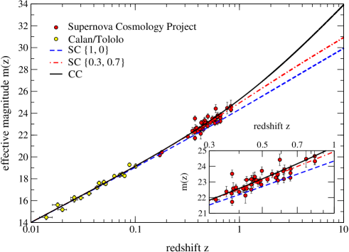
FIG. 1.: $m(z)$- relation for a flat universe model in SC and CC. The data points include those from 42 high-redshift Type Ia supernovae [1]. An optimal fit to these data within the Standard Cosmology requires a cosmological constant $\Omega_{\Lambda}=0.7$, whereas in the Conformal Cosmology presented here no cosmological constant is needed [26].

F Conclusion

We have defined the cosmological parameters $H_{c,0}$, $\Omega_{m,c}$ and $\Omega_{\Lambda,c}$ in the Conformal Cosmology. We have shown how the age of the universe depends on them. The important result of the above derivation of the cosmological parameters in the Conformal Cosmology is the fact, that we can fit the recent Supernova data at $z\sim 1$ in the Hubble diagram (m(z)-relation) in a simple dust case very well and therefore do not need a cosmological constant [26]. Furthermore we gave a prediction for the behaviour at $z>1$ which deviates from the standard FRW cosmology with a non-vanishing $\Lambda$-term. Within this model we suggest as a possible explanation of the recent data from the Supernova Cosmology Project a static (nonexpanding) flat universe where the apparent “acceleration” stems from the evolution of the scalar dilaton field in Conformal General Relativity, when applied to cosmology. This scenario provides alternative views on the origin of standard cosmological data (such as the Cosmic Microwave Background Radiation [24]), which we begin to explore. There is another way to realize the mixing of the dilaton with the standard model Higgs field [25] which was considered recently within the conformal cosmology approach [26] and which slightly modifies the predictions for the magnitude-redshift relation, Fig. 1. However, the conclusion of the present paper, that no cosmological constant is needed for a description of the recent high-redshift supernova data, remains.

List of

Participants of the Workshops on

Quark Matter in Astro- and Particle Physics

Rostock (Germany), November 2000
Dynamical Aspects of the QCD Phase Transition

Trento (Italy), March 2001

Reinhard Alkofer, Reinhard.Alkofer@uni-tuebingen.de,
Universität Tübingen, Institut für Theoretische Physik, Auf der Morgenstelle 14, D-72076 Tübingen, Germany
Danilo Behnke, danilo.behnke@physik.uni-rostock.de, Universität Rostock, Fachbereich Physik, Universitätsplatz 3, D-18051 Rostock, Germany
Michael Beyer, michael.beyer@physik.uni-rostock.de, Universität Rostock, Fachbereich Physik, Universitätsplatz 3, D-18051 Rostock, Germany
David Blaschke, david.blaschke@physik.uni-rostock.de, Universität Rostock, Fachbereich Physik, Universitätsplatz 3, D-18051 Rostock, Germany
Jacques Bloch, bloch@alpha10.tphys.physik.uni-tuebingen.de, Universität Tübingen, Institut für Theoretische Physik, Auf der Morgenstelle 14, D-72076 Tübingen, Germany
Kyrill Bugaev, bugaev@th.physik.uni-frankfurt.de, Universität Frankfurt, Institut fuer Theoretische Physik, Robert-Mayer-Str. 8-10, D- 60325 Frankfurt, Germany
Gerhard Burau, gerhard.burau@physik.uni-rostock.de, Universität Rostock, Fachbereich Physik, Universitätsplatz 3, D-18051 Rostock, Germany
Sergey Dorkin, dorkin@phys.dvgu.ru, Far Eastern State University, Vladivostok 690000, Russia
Alessandro Drago, drago@fe.infn.it, Universita’ di Ferrara, Dipartimento di Fisica, Via Paradiso 12, 44100 Ferrara, Italy
Christian Gocke, chris@darss.mpg.uni-rostock.de, Universität Rostock, Fachbereich Physik, Universitätsplatz 1, D-18051 Rostock, Germany
Kevin L. Haglin, haglin@stcloudstate.edu, Saint Cloud State University, Department of Physics and Astronomy, 720 Fourth Avenue South, MS 313, St. Cloud, MN 56301, USA
Arne Höll, hoell@darss.mpg.uni-rostock.de, Universität Rostock, Fachbereich Physik, Universitätsplatz 3, D-18051 Rostock, Germany
Jörg Hüfner, joerg.huefner@urz.uni-heidelberg.de, Universität Heidelberg, Institut für Theoretische Physik, Philosophenweg 19, D-69120 Heidelberg, Germany
Valery Ivanov, vivanov@cv.jinr.ru, Bogoliubov Laboratory of Theoretical Physics, Joint Institute for Nuclear Research, 141980 Dubna, Russia
Yura Kalinovsky, kalinov@cv.jinr.dubna.su, Laboratory of Information Technologies, Joint Institute for Nuclear Research, 141980 Dubna, Russia
Dubravko Klabucar, klabucar@phy.hr, Zagreb University, Physics Department of Faculty of Science, Bijenicka c. 32, HR-10000 Zagreb, Croatia
Kurt Langfeld, kurt.langfeld@uni-tuebingen.de, Institut für Theoretische Physik, Universität Tübingen, Auf der Morgenstelle 14, D-72076 Tübingen, Germany
Stefan Leupold, stefan.leupold@theo.physik.uni-giessen.de, Universität Giessen, Institut fuer Theoretische Physik I, Heinrich-Buff-Ring 16, D-35392 Giessen, Germany

Gouranga C. Nayak, nayak@th.physik.uni-frankfurt.de, Universität Frankfurt, Institut fuer Theoretische Physik, Robert-Mayer-Str. 8-10, D-60325 Frankfurt, Germany
Viktor Pervushin, pervush@thsun1.jinr.ru, Bogoliubov Laboratory of Theoretical Physics, Joint Institute for Nuclear Research, 141980 Dubna, Russia
Janos Polonyi, polonyi@fresnel.u-strasbg.fr, University Strasbourg, 3 rue de l’Universite, 67084 Strasbourg Cedex, France
Sasha Prozorkevich, smol@ns.ssu.runnet.ru, Saratov State University 410026, Moskovskaya, 155 Physics Department, Russia
Hugo Reinhardt, reinhardt@uni-tuebingen.de, Universität Tübingen, Institut für Theoretische Physik, Auf der Morgenstelle 14, D-72076 Tübingen, Germany
Gerd Röpke, gerd@darss.mpg.uni-rostock.de, Universität Rostock, Fachbereich Physik, Universitätsplatz 3, D-18051 Rostock, Germany
Maria Ruivo, Maria@teor.fis.uc.pt, Departamento de Fisica, Universidade de Coimbra, P-3004-516 Coimbra, Portugal
Sebastian Schmidt,
basti@pion20.tphys.physik.uni-tuebingen.de, Universität Tübingen, Institut für Theoretische Physik, Auf der Morgenstelle 14, D-72076 Tübingen, Germany
Norberto N. Scoccola, scoccola@tandar.cnea.gov.ar, Physics Dept., Comision Nac de Energia Atomica, Physics Dept. - Lab. TANDAR Comision Nac. de Energia Atomica, Av. Libertador 8250, (1429) Ciudad de Buenos Aires, Argentina
Julien Serreau, Julien.Serreau@th.u-psud.fr, Université Paris-Sud, Laboratoire de Physique Theorique, Bâtiment 210, 91405 Orsay Cedex, France
Jonivar Skullerud, jonivar@mail.desy.de, DESY Theory Group, Notkestraße 85, D–22603 Hamburg, Germany
S. A. Sofianos, sofiasa@kiaat.unisa.ac.za, University of South Africa, Dept. of Physics, Pretoria 0003, South Africa
Markus Thoma, markus.thoma@cern.ch, CERN, Theory Division, CH-1211 Geneva 23, Switzerland
Pengfei Zhuang, zhuang@tphys.uni-heidelberg.de, Universität Heidelberg, Institut für Theoretische Physik, Philosophenweg 19, D-69120 Heidelberg, Germany

REFERENCES

- [1] T. Kugo and I. Ojima, Prog. Theor. Phys. Supl. 66 (1979) 1.
- [2] N. Nakanishi and I. Ojima, Covariant Operator Formalism of Gauge Theories and Quantum Gravity, World Scientific Lecture Notes in Physics, Vol. 27, 1990.
-
[3]
R. Oehme and W. Zimmermann,
Phys. Rev. D21 (1980) 471; ibid., 1661;
R. Oehme, Phys. Rev. D42 (1990) 4209, Phys. Lett. B252 (1990) 641. -
[4]
K. Nishijima, Int. J. Mod. Phys. A9 (1994) 3799,
ibid., A10 (1995) 3155;
see also, Czech. J. Phys. 46 (1996) 1. -
[5]
R. Alkofer and L. v. Smekal, The Infrared Behavior of QCD Green’s
Functions,
Physics Reports (2001), in press [hep-ph/0007355]; and references therein. - [6] R. Haag, Local Quantum Physics, Springer, 1996; and references therein.
- [7] T. Kugo, at Int. Symp. BRS Sym., Kyoto, Sep. 1995, hep-th/9511033.
- [8] F. Lenz, H. Naus, K. Otha and M. Thies, Ann. Phys. 233 (1994) 17; ibid., 51.
- [9] M. Stingl, Z. Phys. A353 (1996) 423 [hep-th/9502157].
-
[10]
L. v. Smekal, R. Alkofer and A. Hauck, Phys. Rev. Lett. 79 (1997) 3591;
L. v. Smekal, A. Hauck and R. Alkofer, Ann. Phys. 267 (1998) 1. - [11] V. N. Gribov, Nucl. Phys. B139 (1978) 1.
- [12] D. Zwanziger, Nucl. Phys. B378 (1992) 525; ibid., B412 (1994) 657.
- [13] F. Bonnet, P. O. Bowman, D. B. Leinweber and A. G. Williams, Phys. Rev. D62 (2000) 051501.
-
[14]
For applications of DSEs to QCD at finite temperature and density, see
C. D. Roberts and S. M. Schmidt, Prog. Part. Nucl. Phys. 45 (2000) S1. -
[15]
D. Atkinson and J. C. R. Bloch,
Mod. Phys. Lett. A13 (1998) 1055;
C. Lerche and L. v. Smekal, in preparation. - [16] P. Watson and R. Alkofer, Phys. Rev. Lett. 86 (2001) , in press [hep-ph/0102332].
- [17] A. Hauck, L. v. Smekal and R. Alkofer, Comp. Phys. Comm. 112 (1998) 166.
- [18] D. Atkinson and J. C. R. Bloch, Phys. Rev. D58 (1998) 094036.
- [19] S. Furui and H. Nakajima, hep-lat/0012017; and references therein.
- [20] J. E. Mandula, Phys. Rep. 315 (1999) 273; and references therein.
- [21] J. E. Mandula and M. Ogilvie, Phys. Lett. B185 (1987) 127.
-
[22]
A. Nakamura et al.,
in RCNP Confinement 1995, pp. 90-95, hep-lat/9506024;
H. Aiso et al., Nucl. Phys. (Proc. Suppl.) B53 (1997) 570. - [23] D.B. Leinweber, J.I. Skullerud, A.G. Williams and C. Parrinello, Phys. Rev. D58 (1998) 031501; see also: K. Langfeld, these proceedings [hep-lat/0104003].
- [24] A. Cucchieri, Nucl. Phys. B508 (1997) 353; in Understanding Deconfinement in QCD, World Scientific (1999), hep-lat/9908050.
- [25] C. Alexandrou, P. de Forcrand and E. Follana, Phys. Rev. D63 (2001) 094504; hep-lat/0009003.
- [26] H. Suman and K. Schilling, Phys. Lett. B373 (1996) 314.

REFERENCES

- [1] G. S. Bali, K. Schilling and C. Schlichter, Phys. Rev. D51 (1995) 5165; [hep-lat/9409005].
-
[2]
D. B. Kaplan, Phys. Lett. B288 (1992) 342,
[hep-lat/9206013].
R. Narayanan and H. Neuberger, Phys. Lett. B302 (1993) 62, [hep-lat/9212019]; Nucl. Phys. B412 (1994) 574, [hep-lat/9307006].
P. M. Vranas, Nucl. Phys. Proc. Suppl. 94 (2001) 177, [hep-lat/0011066]. - [3] I. M. Barbour [UKQCD Collaboration], Nucl. Phys. A642 (1998) 251.
-
[4]
J. Engels, O. Kaczmarek, F. Karsch and E. Laermann,
Nucl. Phys.B558 (1999) 307; [hep-lat/9903030].
K. Langfeld and G. Shin, Nucl. Phys. B572 (2000) 266, [hep-lat/9907006]. - [5] C. D. Roberts and A. G. Williams, Prog. Part. Nucl. Phys. 33 (1994) 477, [hep-ph/9403224].
- [6] R. Alkofer and L. von Smekal, Phys. Rept. 353 (2001) 281.
- [7] C. D. Roberts and S. M. Schmidt, Prog. Part. Nucl. Phys. 45S1 (2000) 1, [nucl-th/0005064].
-
[8]
L. Baulieu and M. Schaden,
Int. J. Mod. Phys.A13 (1998) 985, [hep-th/9601039].
M. Schaden and A. Rozenberg, Phys. Rev. D57 (1998) 3670, [hep-th/9706222]. -
[9]
L. von Smekal, R. Alkofer and A. Hauck,
Phys. Rev. Lett. 79 (1997) 3591, [hep-ph/9705242].
L. von Smekal, A. Hauck and R. Alkofer, Annals Phys. 267 (1998) 1, [hep-ph/9707327]. - [10] Chr. Fischer, private communications.
- [11] D. Atkinson and J. C. Bloch, Phys. Rev.D58 (1998) 094036, [hep-ph/9712459].
- [12] D. Atkinson and J. C. Bloch, Mod. Phys. Lett. A13 (1998) 1055, [hep-ph/9802239].
-
[13]
A. Cucchieri,
Nucl.Phys. B508 (1997) 353, [hep-lat/9705005].
A. Cucchieri and T. Mendes, Nucl. Phys. Proc. Suppl. 53 (1997) 811, [hep-lat/9608051]. -
[14]
F. D. Bonnet, P. O. Bowman, D. B. Leinweber,
A. G. Williams and J. M. Zanotti, hep-lat/0101013.
F. D. Bonnet, P. O. Bowman, D. B. Leinweber and A. G. Williams, Phys. Rev.D62 (2000) 051501, [hep-lat/0002020]. - [15] D. Zwanziger, Nucl. Phys. B412 (1994) 657.
-
[16]
L. Del Debbio, M. Faber, J. Greensite and S. Olejnik,
Phys. Rev.D55 (1997) 2298, [hep-lat/9610005].
L. Del Debbio, M. Faber, J. Giedt, J. Greensite and S. Olejnik, Phys. Rev.D58 (1998) 094501, [hep-lat/9801027]. - [17] K. Langfeld, H. Reinhardt and O. Tennert, Phys. Lett. B419 (1998) 317, [hep-lat/9710068].
-
[18]
K. Langfeld, O. Tennert, M. Engelhardt and H. Reinhardt,
Phys. Lett.B452 (1999) 301, [hep-lat/9805002].
M. Engelhardt, K. Langfeld, H. Reinhardt and O. Tennert, Phys. Rev. D61 (2000) 054504, [hep-lat/9904004]. - [19] P. de Forcrand and M. D’Elia, Phys. Rev. Lett. 82 (1999) 4582, [hep-lat/9901020].

REFERENCES

- [1] L.D. Faddeev 1969 Teor. Mat. Fiz. 1 (1969) 3 (in Russian).
- [2] L. Faddeev and V. Popov, Phys. Lett. 25 B (1967) 29.
- [3] S.Gogilidze, N. Ilieva, and V. Pervushin, Int.J.Theor.Phys.A A14 (1999) 3594.
-
[4]
B.M. Barbashov, V. N. Pervushin, and M. Pawlowski,
Reparameterization-invariant dynamics of relativistic systems, Proc. of the Seminar ”Modern Problems of Theoretical Physics”, Dubna, April 26, 2000, Editors: A.V. Efremov, V.V. Nesterenko (Dubna JINR D-2-2000-201) pp 37-103. - [5] W. Heisenberg, W. Pauli, Z.Phys. 56 (1929) 1; ibid 59 (1930) 166.
- [6] P.A.M. Dirac, Can. J. Phys. 33 (1955) 650.
- [7] W. Kummer, Nuovo Cimento 31 (1964) 219.
-
[8]
Yu.L. Kalinovskii et al., Sov.J.Nucl.Phys. 49 (6) (1989) 1059;
V.N. Pervushin, Nucl. Phys. (Proc.Supp.) 15 (1990) 197. - [9] B. Zumino, J. Math. Phys. 1 (1960) 1.
-
[10]
M.A. Markov, J.Phys. (USSR) 2 (1940) 453;
H. Yukawa, Phys.Rev.77 (1950) 219. - [11] A. Eddington, Relativistic Theory of Protons and Electrons (Cambridge University Press, 1936).
- [12] L.D. Faddeev, A.A. Slavnov, Gauge fields: Introduction to Quantum Theory Benjamin-Gummings, (1984).
- [13] V.N. Pervushin, Teor. Mat. Fiz. 45 (1980) 327, English translation in Theor. Math. Phys. 45 (1981) 1100.
- [14] T.T. Wu and C.N. Yang, Phys.Rev. D12 (1975) 3845.
- [15] L.D. Faddeev and A.J. Niemi, Nature (1997) 58.
- [16] M.K. Prasad and C.M. Sommerfield, Phys. Rev. Lett. 35 (1975) 760.
- [17] V.N. Pervushin, Riv. Nuovo Cim. 8, N 10 (1985) 1; A.M. Khvedelidze and V.N. Pervushin, Helv. Phys. Acta 67 (1994) 637.
- [18] D. Blaschke, V. Pervushin, G. Röpke, Proc. of Int. Seminar Physical variables in Gauge Theories Dubna, September 21-25, 1999 (E2-2000-172, Dubna, 2000 Edited by A. Khvedelidze, M. Lavelle, D. McMullan, and V. Pervushin) p.49; [hep-th/0006249].
- [19] V.N. Pervushin and Nguyen Suan Han, Can.J.Phys. 69 (1991) 684.
- [20] G. ’t Hooft, Phys.Rep. 142 (1986) 357; Monopoles, Instantons and Confinement, [hep-th/0010225].
- [21] Yu. Kalinovsky et.al., Few-Body System 10 (1991) 87.
- [22] A.A. Bogoubskaya, et.al., Acta Phys. Polonica 21 (1990) 139.
- [23] V.N. Gribov, Nucl.Phys. B139 (1978) 1.
- [24] S. Schweber, An Introduction to Relativistic Quantum Field Theory (1961) (Row, Peterson and Co Evanston, Ill., Elmsford, N.Y).

REFERENCES

- [1] A. Chodos, R. L. Jaffe, K. Johnson, C. B. Thorne, V. F. Weisskopf, Phys. Rev. D 9 (1974) 3471; A. Chodos, R. L. Jaffe, K. Johnson, C. B. Thorne, Phys. Rev. D 10 (1974) 2599.
- [2] G. ’tHooft, in High Energy Physics, EPS International Conference, Palermo, 1975, ed. A. Zichichi, 1976; S. Mandelstam, Phys. Rep. C 23 (1976) 245; G. Parisi, Phys. Rev. D 11 (1975) 971; H. B. Nielsen, P. Olesen, Nucl. Phys. B 61 (1973) 45.
- [3] H. G. Dosch, Phys. Lett. B 190 (1987) 555; H. G. Dosch, Y. Simonov, Phys. Lett. B 205 (1988) 339; Y. Simonov, Yad. Fiz. 48 (1988) 1381.
- [4] K. Johnson, L. Lellouch, J. Polonyi, Nucl. Phys. B 367 (1991) 675.
- [5] T. Reisz, Nucl. Phys. B 318 (1989) 417.
- [6] J. Polonyi, in the Proceedings of the International School of Physics, Enrico Fermi, Course CXXX, on Selected Topics in Nonperturbative QCD, ed. A. Di Giacomo, D. Diakonov, Soc. It. di Fisica, 1996.
- [7] J. Polonyi, Phys. Lett. B 213 (1988) 340; in Quark-Gluon Plasma, edt. R. Hwa, World Scientific, 1988.
- [8] W. Greiner, B. Müller, J. Rafelski, Quantum Electrodynamics of Strong Fields, Springer (1985).
- [9] V. N. Gribov, Eur. Phys. J. C 10 (105) 91.
- [10] M. Oleszczuk, J. Polonyi, Canonical versus Grand Canonical Ensembles in QCD, MIT preprint.
- [11] M. Faber, O. Borisenko, G. Zinovev, Nucl. Phys. B 444 (1995) 563.
- [12] V. Pervushin, Riv. Nuovo Cimento 8 (1985) 1.
- [13] J. Polonyi, K. Szlachanyi, Phys. Lett. B 110 (1982) 395.
- [14] J. Alexandre, V. Branchina, J. Polonyi, Phys. Rev. D 58 (1998) 16002.
- [15] J. Alexandre, V. Branchina, J. Polonyi, Phys. Lett. B 445 (1999) 351.
- [16] R. Shankar, Rev. Mod. Phys. 66 (1944) 129.
- [17] E. Manousakis, J. Polonyi, Phys. Rev. Lett. 58 (1987) 847.
- [18] M. Oleszczuk, J. Polonyi, Ann. Phys. 277 (1993) 76.

REFERENCES

- [1] M. Alford, K. Rajagopal and F. Wilczek, Phys. Lett. B422, 247 (1998), [hep-ph/9711395].
- [2] R. Rapp, T. Schäfer, E. Shuryak and M. Velkovsky, Phys. Rev. Lett. 81, 53 (1998), [hep-ph/9711396].
- [3] M. Alford, K. Rajagopal and F. Wilczek, Nucl. Phys. B537, 443 (1999), [hep-ph/9804403].
- [4] K. Rajagopal and F. Wilczek, The condensed matter physics of QCD, in At the Frontier of Particle Physics: Handbook of QCD, edited by M. Shifman, p. 2061, Singapore, 2001, World Scientific, [hep-ph/0011333].
- [5] S. Hands, hep-lat/0109034.
- [6] E. B. Gregory, S.-H. Guo, H. Kröger and X.-Q. Luo, Phys. Rev. D62, 054508 (2000), [hep-lat/9912054].
- [7] X.-Q. Luo, E. B. Gregory, S.-H. Guo and H. Kröger, QCD at finite density, In Luo and Gregory [31], pp. 138–149, [hep-ph/0011120].
- [8] M. Alford, A. Kapustin and F. Wilczek, Phys. Rev. D59, 054502 (1999), [hep-lat/9807039].
- [9] M.-P. Lombardo, Nucl. Phys. Proc. Suppl. 83, 375 (2000), [hep-lat/9908006].
- [10] A. Hart, M. Laine and O. Philipsen, Phys. Lett. B505, 141 (2001), [hep-lat/0010008].
- [11] J. Engels, O. Kaczmarek, F. Karsch and E. Laermann, Nucl. Phys. B558, 307 (1999), [hep-lat/9903030].
- [12] S. Chandrasekharan, Nucl. Phys. Proc. Suppl. 94, 71 (2001), [hep-lat/0011022].
- [13] D. Son and M. Stephanov, Phys. Rev. Lett. 86, 592 (2001), [hep-ph/0005225].
- [14] S. Hands, B. Kogut, S. Morrison and D. Sinclair, Nucl. Phys. Proc. Suppl. 94, 457 (2001), [hep-lat/0010028].
- [15] P. Hasenfratz and F. Karsch, Phys. Lett. B125, 308 (1983).
- [16] J. Kogut, M. Stephanov, D. Toublan, J. Verbaarschot and A. Zhitnitsky, Nucl. Phys. B582, 477 (2000), [hep-ph/0001171].
- [17] S. Hands et al., Eur. Phys. J. C17, 285 (2000), [hep-lat/0006018].
- [18] S. Morrison and S. Hands, Two colours QCD at nonzero chemical potential, in Strong and Electroweak Matter, Copenhagen, 1998, p. 364, 1999, [hep-lat/9902012].
- [19] R. Aloisio, V. Azcoiti, G. Di Carlo, A. Galante and A. Grillo, Diquark condensation in two colour QCD, In Luo and Gregory [31], pp. 123–131, [hep-lat/0007018].
- [20] V. Azcoiti, V. Laliena and X.-Q. Luo, Phys. Lett. B354, 111 (1995), [hep-th/9509091].
- [21] S. Hands and S. Morrison, Diquark condensation in dense matter: A lattice perspective, in Understanding Deconfinement in QCD, edited by D. Blaschke et al., p. 31, Singapore, 2000, World Scientific, [hep-lat/9905021].
- [22] R. Aloisio, V. Azcoiti, G. Di Carlo, A. Galante and A. F. Grillo, Phys. Lett. B493, 189 (2000), [hep-lat/0009034].
- [23] R. Aloisio, V. Azcoiti, G. Di Carlo, A. Galante and A. Grillo, Nucl. Phys. B606, 322 (2001), [hep-lat/0011079].
- [24] E. Bittner, M.-P. Lombardo, H. Markum and R. Pullirsch, Nucl. Phys. Proc. Suppl. 94, 445 (2001), [hep-lat/0010018].
- [25] B. Allés, M. D’Elia, M. Lombardo and M. Pepe, Nucl. Phys. Proc. Suppl. 94, 441 (2001), [hep-lat/0010068].
- [26] Y. Liu, O. Miyamura, A. Nakamura and T. Takaishi, Simulation of SU(2) dynamical fermion at finite chemical potential and at finite temperature, In Luo and Gregory [31], pp. 132–137, [hep-lat/0009009].
- [27] S. Muroya, A. Nakamura and C. Nonaka, Nucl. Phys. Proc. Suppl. 94, 469 (2001), [hep-lat/0010073].
- [28] S. Hands, I. Montvay, M. Oevers, L. Scorzato and J. Skullerud, Nucl. Phys. Proc. Suppl. 94, 461 (2001), [hep-lat/0010085].
- [29] I. Montvay, Nucl. Phys. B466, 259 (1996), [hep-lat/9510042].
- [30] I. Montvay, Multi-bosonic algorithms for dynamical fermion simulations, in Molecular dynamics on parallel computers, World Scientific, 2000, [hep-lat/9903029].
- [31] X.-Q. Luo and E. B. Gregory, editors, Non-perturbative methods and lattice QCD, Guangzhou, 2000 (World Scientific, Singapore, 2001).

REFERENCES

- [1] P. Sprangle, A. Esarey, A. Ting, Phys. Rev. Lett. 64 (1990) 2011.
- [2] P. Gibbon, E. Förster, Plasma Phys. Control. Fusion 38 (1996) 769.
- [3] B. Bezzerides, D.F. DuBois, Ann. Phys. 70 (1972) 10.
- [4] S.R. de Groot, W.A. van Leeuwen and Ch.G. van Weert, Relativistic Kinetic Theory (North-Holland, Amsterdam, 1980).
- [5] S. Ochs, U. Heinz, Ann. Phys. 266 (1998) 351.
- [6] N.N. Bogoliubov, Dokl. Akad. Nauk SSSR 81 (1951) 757.
- [7] G.N. Fleming, Phys. Rev. B137 (1965) 188.
- [8] G.N. Fleming, J. Math. Phys. 7 (1966) 1959.
- [9] A. Höll, V.G. Morozov, G. Röpke, in preparation for Physica A (2001).
- [10] E.P. Wigner, Götting. Nachrichten 31 (1932) 546.
- [11] D. Vasak, M. Gyulassy, H.-T. Elze, Ann. Phys. 173 (1987) 462.
- [12] D.N. Zubarev, V.G. Morozov, G. Röpke, Statistical Mechanics of Nonequilibrium Processes, vol. 1 (Akademie Verlag GmbH, Berlin, 1996).
- [13] I. Bialynicki-Birula, P. Górnicki, J. Rafelski, Phys. Rev. D44 (1991) 1825.

REFERENCES

- [1] R. S. Bhalerao and G. C. Nayak, Phys. Rev. C61 (2000) 054907.
- [2] H-T. Elze and U. Heinz, Phys. Rep. 183 (1989) 81.
- [3] S.K. Wong, Nuovo Cimento A 65 (1970) 689.
- [4] J. Schwinger, Phys. Rev. 82 (1951) 664.
- [5] C. Itzykson and J. Zuber, Quantum Field Theory (McGraw-Hill Inc., 1980).
- [6] G. C. Nayak and W. Greiner, [hep-th/0001009].
- [7] B. S. DeWitt, Phys. Rev. 162 (1967) 1195 and 1239; in Dynamic theory of groups and fields (Gordon and Breach, 1965).
- [8] G. ’t Hooft, Nucl. Phys. B62 (1973) 444.
- [9] L. F. Abbott, Nucl. Phys. B185 (1981) 189.
- [10] D. D. Dietrich, G. C. Nayak and W. Greiner, [hep-th/0007139],submitted to PRD; [hep-ph/0009178], submitted to PRD.

REFERENCES

- [1] S.A. Bass, M. Gyulassy, H. Stöcker and W. Greiner, J. Phys. G G25 (1999) R1; S. Scherer et al., Prog. Part. Nucl. Phys. 42 (1999) 279; U. Heinz and M. Jacob, “Evidence for a new state of matter: An assessment of the results from the CERN lead beam programme,” [nucl-th/0002042].
- [2] L.V. Gribov and M.G. Ryskin, Phys. Rept. 189 (1990) 29; T.S. Biro, C. Gong, B. Müller and A. Trayanov, Int. J. Mod. Phys. C5 (1994) 113; L. McLerran and R. Venugopalan, Phys.Rev. D49 (1994) 2233; ibid 3352.
- [3] B. Andersson, G. Gustafson, G. Ingelman and T. Sjöstrand, Phys. Rept. 97 (1983) 33.
- [4] X. Wang and M. Gyulassy, Phys. Rev. D44 (1991) 3501.
- [5] K. Geiger, Phys. Rept. 258 (1995) 237.
- [6] B. Andersson, G. Gustafson and B. Nilsson-Almquist, Nucl. Phys. B 281 (1987) 289; K. Werner, Phys. Rept. 232 (1993) 87; S.A. Bass et al., Prog. Part. Nucl. Phys. 41 (1998) 225.
- [7] A. Casher, H. Neuberger and S. Nussinov, Phys. Rev. D20 (1979) 179.
- [8] J. Schwinger, Phys. Rev. 82 664 (1951) 664; W. Greiner, B. Müller, and J. Rafelski, Quantum Electrodynamics of Strong Fields (Springer-Verlag, Berlin, 1985).
- [9] Y. Kluger, J.M. Eisenberg, B. Svetitsky, F. Cooper and E. Mottola, Phys. Rev. Lett. 67 (1991) 2427; K. Kajantie and T. Matsui, Phys. Lett. B164 (1985) 373; A. Bialas, W. Czyż, A. Dyrek and W. Florkowski, Nucl. Phys. B296 (1988) 611. M.A. Lampert and B. Svetitsky, Phys. Rev. D61 (2000) 034011.
- [10] C.D. Roberts and S.M. Schmidt, Prog. Part. Nucl. Phys. 45 (2000) S1.
- [11] Y. Kluger, E. Mottola, and J.M. Eisenberg, Phys. Rev. D58 (1998) 125015.
- [12] F. Cooper and E. Mottola, Phys. Rev. D36 (1987) 3114; ibid D40 (1989) 456; M. Herrmann and J. Knoll, Phys. Lett. B234 (1990) 437; D. Boyanovsky, H.J. de Vega, R. Holman, D.S. Lee and A. Singh, Phys. Rev. D51 (1995) 4419; W. Dittrich and H. Gies, Springer Tracts Mod. Phys. 166 (2000) 1.
- [13] J. Rau and B. Müller, Phys. Rept. 272 (1996) 1.
- [14] S.M. Schmidt D. Blaschke, G. Röpke, S.A. Smolyansky, A.V. Prozorkevich and V.D. Toneev, Int. J. Mod. Phys. E7 (1998) 709.
- [15] S.A. Smolyansky, G. Röpke, S.M. Schmidt, D. Blaschke, V.D. Toneev and A.V. Prozorkevich, [hep-ph/9712377]; S.M. Schmidt, A.V. Prozorkevich, and S.A. Smolyansky, Creation of boson and fermion pairs in strong fields, Proceedings ’V. Workshop on Nonequilibrium Physics at Short Time Scales’, April 27-30, 1998, hep-ph/9809233.
- [16] S.M. Schmidt, D. Blaschke, G. Röpke, A.V. Prozorkevich, S.A. Smolyansky and V.D. Toneev, Phys. Rev. D59 (1999) 094005.
- [17] J.C.R. Bloch, V.A. Mizerny, A.V. Prozorkevich, C.D. Roberts, S.M. Schmidt, S.A. Smolyansky, D.V. Vinnik, Phys. Rev. D60 (1999) 116011.
- [18] J.C.R. Bloch, C.D. Roberts and S.M. Schmidt, Phys. Rev. D 61 (2000) 117502.
- [19] J.M. Eisenberg, Found. Phys. 27 (1997) 1213.
- [20] N.K. Glendenning and T. Matsui, Phys. Lett. B141 (1984) 419; M. Gyulassy and T. Matsui, Phys. Rev. D 29 (1984) 419; K. Kajantie, R. Raitio and P.V. Ruuskanen, Nucl. Phys. B222 (1983) 152; G. Baym, B.L. Friman, J.P. Blaizot, M. Soyeur and W. Czyż, Nucl. Phys. A 407 (1983) 541.
- [21] G.C. Nayak, A. Dumitru, L. McLerran and W. Greiner, “Equilibration of the gluon-minijet plasma at RHIC and LHC,” [hep-ph/0001202].
- [22] C.D. Roberts and A.G. Williams, Prog. Part. Nucl. Phys. 33 (1994) 477.
- [23] J. I. Skullerud and A. G. Williams, [hep-lat/0007028].
- [24] C.D. Roberts and S.M. Schmidt, “Temperature, chemical potential and the -meson,” in Proc. of the International Workshop XXVIII on Gross Properties of Nuclei and Nuclear Excitations, edited by M. Buballa, W. Nörenberg, B.-J. Schaefer and J. Wambach (GSI mbH, Darmstadt, 2000), pp. 185-191.
- [25] D. Blaschke, C.D. Roberts and S.M. Schmidt, Phys. Lett. B425 (1998) 232.
- [26] P. Maris and C.D. Roberts, Phys. Rev. C56 (1997) 3369.

REFERENCES

- [1] T. Matsui and H. Satz, Phys. Lett. B178 (1986) 416.
- [2] B.Z. Kopeliovich and B.G. Zakharov, Phys. Rev. D44 (1991) 3466.
- [3] J.B. Kogut and D.E. Soper, Phys. Rev. D1 (1970) 2901;
- [4] J.M. Bjorken, J.B. Kogut and D.E. Soper, D3 (1971) 1382
- [5] A.B. Zamolodchikov, B.Z. Kopeliovich and L.I. Lapidus, JETP Lett. 33 (1981) 595.
- [6] K. Golec-Biernat and M. Wüsthoff, Phys. Rev. D53 (1999) 014017; [hep-ph/9903358].
- [7] B. Kopeliovich, A. Schäfer and A. Tarasov, Nonperturbative Effects in Gluon Radiation and Photoproduction of Quark Pairs, to appear in Phys.Rev. D; [hep-ph/9908245].
- [8] W. Lucha and F.F. Schöberl, Int.J.Mod.Phys. C10 (1999) 607-620; [hep-ph/9811453].
- [9] W. Buchmüller and S.-H.H. Tye, Phys. Rev. D24 (1981) 132.
- [10] E. Eichten, K. Gottfried, T. Konoshita, K.D. Lane and T.-M. Yan, Phys. Rev. D17 (1978) 3090; Phys. Rev. D21 (1980) 203.
- [11] C. Quigg and J.L. Rosner, Phys.Lett. B71 (1977) 153.
- [12] A. Martin, Phys.Lett. B93 (1980) 338.
- [13] O. Benhar, B.Z. Kopeliovich, Ch. Mariotti, N.N. Nikolaev and B.G. Zakharov, Phys. Rev. Lett. 69 (1992) 1156.
- [14] M.V.Terent’ev, Sov.J. Nucl. Phys. 24 (1976) 106.
- [15] P. Hoyer and S. Peigné, Phys. Rev. D61 (2000) 031501(R)
- [16] H.J. Melosh, Phys. Rev. D9 (1974) 1095; W. Jaus, Phys. Rev. D41 (1990) 3394.
- [17] H1 Collab., C. Adloff et al., DESY 00-037; [hep-ex/0003020].
- [18] E401 Collab., M. Binkley et al., Phys. Rev. Lett. 48 73 (1982).
- [19] E516 Collab., B. H. Denby et al., Phys. Rev. Lett. 52 795 (1984).
- [20] ZEUS Collab., J. Breitweg et al., Z. Phys. C75 215 (1997).
- [21] K. Suzuki et al., Validity of the Color Dipole Approximation for Diffractive Production of Heavy Quarkonium, [hep-ph/0005250].
- [22] U. Camerini et al., Phys. Rev. Lett. 35 483 (1975).
- [23] NA14 Collab., R. Barate et al., Z. Phys. C33 505 (1987).
- [24] E401 Collab., M. Binkley et al., Phys. Rev. Lett. 50 302 (1983).
- [25] EMC Collab., J.J. Aubert et al., Nucl. Phys. B213 1 (1983).
- [26] NMC Collab., P. Amaudraz et al., Nucl. Phys. B371 553 (1992).
- [27] H1 Collab., C. Adloff et al., Phys. Lett. B421 385 (1998); [hep-ex/9711012]. Phys. Rev. Lett. 81 (1998) 762
- [28] H. G. Dosch, F. S. Navarra, M. Nielsen, M. Rueter, Phys. Lett. B466 (1999) 363; H.G. Dosch, T. Gousset, G. Kulzinger, H.J. Pirner, Phys.Rev. D55 (1997) 2602

REFERENCES

- [1] M.C. Abreu et al. (NA50 Collab.), Phys. Lett. B477, 28 (2000).
- [2] T. Matsui, H. Satz, Phys. Lett. B178, 416 (1986).
- [3] R. Redmer, Phys. Rep. 282, 35 (1997).
- [4] F. Karsch, M.T. Mehr, H. Satz, Z. Phys. C37, 617 (1988).
- [5] G. Röpke, D. Blaschke, H. Schulz, Phys. Lett. B202, 479 (1988).
- [6] G. Röpke, D. Blaschke, H. Schulz, Phys. Rev. D38, 3589 (1988).
- [7] D. Blaschke, G. Burau, Yu. Kalinovsky, Mott dissociation of D-mesons at the chiral phase transition and anomalous J/ suppression, in: Progress in Heavy Quark Physics 5, Dubna (2000); [nucl-th/0006071].
- [8] G. Burau, D. Blaschke, Yu. Kalinovsky, Phys. Lett. B506, 297 (2001).
- [9] S.G. Matinyan, B. Müller, Phys. Rev. C58, 2994 (1998).
- [10] Z. Lin, C.M. Ko, Phys. Rev. C62, 034903 (2000).
- [11] K. Haglin, C. Gale, Hadronic Interactions of the J/, [nucl-th/0010017].
- [12] K. Martins, D. Blaschke, E. Quack, Phys. Rev. C51, 2723 (1995).
- [13] P. Braun-Munzinger, K. Redlich, Nucl. Phys. A661, 546 (1999).
- [14] C.M. Ko, B. Zhang, X.F. Zhang, X.-N. Wang, Phys. Lett. B444, 237 (1998).
- [15] C.-Y. Wong, E. Swanson, T. Barnes, Phys. Rev. C62, 045201 (2000).
- [16] D. Blaschke, G. Burau, M. Ivanov, Yu. Kalinovsky, P.C. Tandy, in: Progress in Nonequilibrium Green Functions, Ed. M. Bonitz, World Scientific, Singapore, 2000, p. 392; [hep-ph/0002047].
- [17] J.-C. Itzykson, P.-B. Zuber, Quantum Field Theory, McGraw-Hill, New York, 1980.
- [18] F.E. Close, An Introduction to Quarks and Partons, Academic Press, London, 1979.

REFERENCES

- [1] NA50 Collab., M. C. Abreu et al., Phys. Lett. B477 (2000) 28.
- [2] T. Matsui and H. Satz, Phys. Lett. B178 (1986) 416.
- [3] D. Blaschke, G. Röpke and H. Schulz, Phys. Lett. B233 (1989) 434 ; D. Blaschke, Nucl. Phys. A525 (1991) 296c.
- [4] T. H. Hansson, S. H. Lee and I. Zahed, Phys. Rev. D37 (1988) 2672.
- [5] G. Röpke, D. Blaschke and H. Schulz, Phys. Rev. D38 (1988) 3589.
- [6] D. Kharzeev and H. Satz, Phys. Lett. B334 (1994) 155.
- [7] R. Vogt, M. Prakash, P. Koch and T. H. Hansson, Phys. Lett. B207 (1988) 263.
- [8] K. Martins, D. Blaschke and E. Quack, Phys. Rev. C51 (1995) 2723.
- [9] L.P. Kadanoff and G. Baym, Quantum Statistical Mechanics (Benjamin, New York, 1962).
- [10] T. Barnes and E. S. Swanson, Phys. Rev. D46 (1992) 131.
- [11] D. Blaschke and G. Röpke, Phys. Lett. B299 (1993) 332.
- [12] C. Wong, E. S. Swanson and T. Barnes, Phys. Rev. C62 (2000) 045201.
- [13] S. G. Matinyan and B. Müller, Phys. Rev. C58 (1998) 2994.
- [14] K. L. Haglin, Phys. Rev. C61 (2000) 031902 ; K. L. Haglin and C. Gale, Hadronic interactions of the , [nucl-th/0010017].
- [15] D. B. Blaschke, G. R. G. Burau, M. A. Ivanov, Y. L. Kalinovsky and P. C. Tandy, Dyson-Schwinger equation approach to the QCD deconfinement transition and dissociation, in: Progress in Nonequilibrium Green’s Functions, ed. M. Bonitz (World Scientific, Singapore, 2000) p. 392, [hep-ph/0002047].
- [16] D. Blaschke, Y. L. Kalinovsky, V. N. Pervushin, G. Röpke and S. M. Schmidt, Z. Phys. A346 (1993) 85.
- [17] F. O. Gottfried and S. P. Klevansky, Phys. Lett. B286 (1992) 221.
- [18] D. Blaschke, Y. L. Kalinovsky and P. C. Tandy, Quark deconfinement and meson properties at finite temperature, in: Proc. XIth International Conference Problems of Quantum Field Theory (Dubna, July 1998), eds. B.M. Barbashov, G.V. Efimov and A.V. Efremov (JINR Press, Dubna, 1999) p. 454, [hep-ph/9811476].
- [19] D. Blaschke, Y. L. Kalinovsky, P. Petrow, S. M. Schmidt, M. Jaminon and B. Van den Bossche, Nucl. Phys. A592 (1995) 561.
- [20] Y. B. He, J. Hüfner and B. Z. Kopeliovich, Phys. Lett. B477 (2000) 93.
- [21] D. Blaschke, G. Burau and Y. L. Kalinovsky, Mott dissociation of D mesons at the chiral phase transition and anomalous suppression, in: Proc. Vth International Workshop on Heavy Quark Physics (Dubna, April 2000), [nucl-th/0006071].
- [22] C.-Y. Wong, Phys. Rev. Lett. 76 (1996) 196.
- [23] K. Martins and D. Blaschke, Charmonium dissociation in hot and dense matter, in: Proc. Vth International Workshop on Heavy Quark Physics (Rostock, September 1997), eds. M. Beyer, T. Mannel and H. Schröder (University Press, Rostock, 1998) p. 189, [hep-ph/9802250].
- [24] A. Capella, E. G. Ferreiro and A. B. Kaidalov, Phys. Rev. Lett. 85 (2000) 2080.
- [25] J. Blaizot, M. Dinh and J. Ollitrault, Phys. Rev. Lett. 85 (2000) 4012.
- [26] J. Hüfner, B. Z. Kopeliovich and A. Polleri, Fluctuations of the transverse energy in Pb+Pb collisions and suppression, [nucl-th/0012003].
- [27] S. A. Bass, M. Gyulassy, H. Stöcker and W. Greiner, J. Phys. G25 (1999) R1.
- [28] W. Cassing, E. L. Bratkovskaya and S. Juchem, Nucl. Phys. A674 (2000) 249.
- [29] M. A. Ivanov, Y. L. Kalinovsky and C. D. Roberts, Phys. Rev. D60 (1999) 034018.
- [30] A. Bender, D. Blaschke, Y. Kalinovsky and C. D. Roberts, Phys. Rev. Lett. 77 (1996) 3724.
- [31] C. D. Roberts and S. M. Schmidt, Prog. Part. Nucl. Phys. 45 (2000) 1.
- [32] C. M. Ko, B. Zhang, X. F. Zhang and X. N. Wang, Phys. Lett. B444 (1998) 237.
- [33] P. Braun-Munzinger and K. Redlich, Nucl. Phys. A661 (1999) 546.

REFERENCES

- [1] J. Dukelsky, G. Röpke, P. Schuck, Nucl. Phys. A628 (1998) 17.
- [2] M. Beyer, G. Ropke and A. Sedrakian, Phys. Lett. B376 (1996) 7 [nucl-th/9601038].
- [3] M. Beyer and G. Ropke, [nucl-th/9706021].
- [4] M. Beyer, Few Body Syst. Suppl. 10 (1999) 179 [nucl-th/9809002].
- [5] M. Beyer, W. Schadow, C. Kuhrts and G. Ropke, Phys. Rev. C60 (1999) 034004 [nucl-th/9902074].
- [6] C. Kuhrts, M. Beyer and G. Ropke, Nucl. Phys. A668 (2000) 137 [nucl-th/9908032].
- [7] M. Beyer, C. Kuhrts, G. Ropke and P. D. Danielewicz, [nucl-th/9910058].
- [8] M. Beyer, S. A. Sofianos, C. Kuhrts, G. Ropke and P. Schuck, Phys. Lett. B488 (2000) 247 [nucl-th/0003071].
- [9] C. Kuhrts, M. Beyer, P. Danielewicz and G. Ropke, [nucl-th/0009037].
- [10] E.O. Alt, P. Grassberger, W. Sandhas, Nucl. Phys. B2 (1967) 167.
- [11] W. Sandhas, Acta Physica Austriaca, Suppl. XIII, 679 (1974).
- [12] E.O. Alt, P. Grassberger and W. Sandhas, Report E4-6688, JINR, Dunba 1972 and in Few particle problems in the nuclear interaction eds. I. Slaus et al. (North Holland, Amsterdam 1972) p. 299.
- [13] W. Sandhas, Czech. J. Phys. B25, 251 (1975).
- [14] L.P. Kadanoff, G. Baym, Quantum Theory of Many-Particle Systems (Mc Graw-Hill, New York, 1962); A.L. Fetter, J.D. Walecka, Quantum Theory of Many-Particle Systems, (McGraw-Hill, New York, 1971).
- [15] S. Mattiello, diploma thesis, 2000 (unpublished)
- [16] M. Beyer and S.A. Sofianos, in preparation.
- [17] G. Röpke, A. Schnell, P. Schuck, P. Noziére, Phys. Rev. Lett. 80 (1998) 3177

REFERENCES

- [1] J.P. Bondorf, A.S. Botvina, A.S. Iljinov, I.N. Mishustin, K.S. Sneppen, Phys. Rep. 257 (1995) 131.
- [2] D.H.E. Gross, Phys. Rep. 279 (1997) 119.
- [3] K.C. Chase and A.Z. Mekjian, Phys. Rev. C52 (1995) R2339.
- [4] S. Das Gupta and A.Z. Mekjian, Phys. Rev. C57 (1998) 1361.
- [5] S. Das Gupta, A. Majumder, S. Pratt and A. Mekjian, [nucl-th/9903007].
- [6] S. Das Gupta, A.Z. Mekjian and M.B. Tsang, [nucl-th/0009033].
- [7] K.A. Bugaev, M.I. Gorenstein, I.N. Mishustin and W. Greiner, Phys. Rev. C62 (2000) 044320.
-
[8]
M.I. Gorenstein, V.K. Petrov and G.M. Zinovjev, Phys. Lett.
B106 (1981) 327;
M.I. Gorenstein, W. Greiner and S.N. Yang, J. Phys. G24 (1998) 725. - [9] K.A. Bugaev, M.I. Gorenstein, I.N. Mishustin and W. Greiner, [nucl-th/0007062].
- [10] K.A. Bugaev, M.I. Gorenstein, I.N. Mishustin and W. Greiner, [nucl-th/0011055.
- [11] M.E. Fisher, Physics 3 (1967) 255.

REFERENCES

- [1]
- [2] D. Klabucar, D. Kekez, Phys. Rev. D58 (1998) 096003.
- [3] F. J. Gilman, R. Kauffmann, Phys. Rev. D36 (1987) 2761.
-
[4]
H. F. Jones, M. D. Scadron, Nucl. Phys. B155 (1979) 409;
M. D. Scadron, Phys. Rev. D29 (1984) 2076. - [5] H. Leutwyler, Nucl. Phys. Proc. Suppl. 64 (1998) 223.
- [6] R. Kaiser, H. Leutwyler, [hep-ph/9806336].
- [7] Th. Feldmann, P. Kroll, Eur. Phys. J. C 5 (1998) 327.
- [8] Th. Feldmann, P. Kroll, Phys. Rev. D58 (1998) 057501.
- [9] Th. Feldmann, P. Kroll, B. Stech, Phys. Rev. D58, 114006 (1998).
- [10] Th. Feldmann, P. Kroll, B. Stech, Phys. Lett. B449 (1999) 339.
- [11] Th. Feldmann, Int. J. Mod. Phys. A15 (2000) 159.
- [12] D. Kekez, D. Klabucar, M. D. Scadron, J. Phys. G26 (2000) 1335.
- [13] A. De Rújula, H. Georgi, S. Glashow, Phys. Rev. D12 (1975) 147.
- [14] A. Bramon, M. D. Scadron, Phys. Lett. B234 (1990) 346.
- [15] A. Bramon, R. Escribano, M. D. Scadron, Phys. Lett. B403 (1997) 339; Eur. Phys. J. C7 (1999) 271.
- [16] See e.g. C. Ayala, A. Bramon, Europhys. Lett. 4 (1987) 777 and references therein.
- [17] A. Bramon, M. D. Scadron, Phys. Rev. D40 (1989) 3779.
-
[18]
A. Patrascioiu, M. D. Scadron, Phys. Rev. D22 (1980) 2054;
R. Delbourgo, M. D. Scadron, ibid. D28 (1983) 2345;
S. R. Choudhury, M. D. Scadron, Mod. Phys. Lett. A1 (1986) 535. -
[19]
M. D. Scadron, Rep. Prog. Phys. 44 (1981) 213, see pp. 247, 268;
S. A. Coon, M. D. Scadron, Phys. Rev. C23 (1981) 1150. -
[20]
L. F. Li, H. Pagels, Phys. Rev. D5 (1972) 1509;
N. Paver, M. D. Scadron, ibid. D30 (1984) 1988. - [21] A recent review is: C. D. Roberts, [nucl-th/0007054].
- [22] P. Jain, H. J. Munczek, Phys. Rev. D48 (1993) 5403.
- [23] H. J. Munczek, P. Jain, Phys. Rev. D46 (1992) 438.
- [24] D. Kekez, B. Bistrović, D. Klabucar, Int. J. Mod. Phys. A 14 (1999) 161.
- [25] D. Kekez, D. Klabucar, Phys. Lett. B387 (1996) 14.
- [26] D. Kekez, D. Klabucar, Phys. Lett. B457 (1999) 359.
- [27] J. Gasser, H. Leutwyler, Nucl. Phys. B250 (1985) 465.
- [28] J. Kogut, L. Susskind, Phys. Rev. D10 (1974) 3468; D11 (1975) 3594.
- [29] M. R. Frank, T. Meissner, Phys. Rev. C57 (1998) 345.
- [30] L. v. Smekal, A. Mecke, R. Alkofer, [hep-ph/9707210].
- [31] C. McNeile, C. Michael, Phys. Lett. B491 (2000) 123.
- [32] R. D. Pisarski, F. Wilczek, Phys. Rev. D29 (1984) 338.
- [33] R. Alkofer, P. A. Amundsen, H. Reinhardt, Phys. Lett B218 (1989) 75.
- [34] J. Kapusta, D. Kharzeev, L. McLerran, Phys. Rev. D53 (1996) 5028.
- [35] Z. Huang, X.-N. Wang, Phys. Rev. D53 (1996) 5034.
- [36] J. B. Kogut, J.-F. Lagae, D. K. Sinclair, Phys. Rev. D58 (1998) 054504.
- [37] P. Maris, C. D. Roberts, S. M. Schmidt, P. C. Tandy, [nucl-th/0001064].
- [38] D. Blaschke, G. Burau, Yu. L. Kalinovsky, P. Maris, P. C. Tandy, Int. J. Mod. Phys. A 16 (2001) 2267.
- [39] D. Blaschke et. al., work in progress.

REFERENCES

- [1] F. Karsch and E. Laermann, Phys. Rev. D50, 6459 1994; K. Kanaya, Prog. Theor. Phys. Sup. 129 (1997) 197.
- [2] Y. Nambu and G. Jona-Lasinio, Phys. Rev. 122 (1961) 345; 124 (1961).
- [3] T. Hatsuda and T. Kunihiro, Phys. Rep. 247 (1994) 221; V. Bernard and U. G. Meissner, Nucl. Phys. A489 (1988) 647; S. Klimt, M. Lutz and W. Weise, Phys. Lett. B249 (1990) 386; S.P. Klevansky Rev. Mod. Phys. 64 (1992) 649 (1992); M.C. Ruivo et al. Nucl. Phys. A575 (1994) 460; J. Cugnon, M. Jaminon and B. van den Bossche Nucl. Phys. A598 (1996) 515; M. Fiolhais et al., Phys. Rev. C56 (1997) 331.
- [4] M.C. Ruivo and C.A. Sousa, Phys. Lett. B385 (1996) 39.
- [5] M.C. Ruivo, C.A. Sousa and C. Providência, Nucl. Phys. A651 (1999) 59.
- [6] C.A. Sousa and M.C. Ruivo, Nucl. Phys., A625 (1997) 713.
- [7] W. Broniowski and B.Hiller, Nucl. Phys., A643 (1998) 161.
- [8] M. Buballa and M. Oertel, Nucl. Phys. A642 (1998) 39c; Phys. Lett. B457 (1999) 261.
- [9] M. Alford, K. Rajagopal and F. Wilczek, Phys. Lett. B422 (1998) 247.
- [10] D. Blaschke and P.C. Tandy, in Understanding Deconfinemente in QCD, Eds. D. Blaschke, F. Karsh and C. Roberts, World. Sientific, Singapore (2000) 218.
- [11] D.B. Kaplan and A.E. Nelson, Phys. Lett. B175 (1986) 57; B192 (1987) 193.
- [12] T. Waas, M. Rho and W. Weise, Nucl. Phys., A617 (1997) 449; M. LutzPhys. Lett. B426 (1998) 12.
- [13] W. Cassing and E.L. Bratkovskaya, Phys. Rep. 308 (1999) 65.
- [14] J. Schaffner et al., Phys. Lett. B334 (1994) 268.
- [15] E. Friedmann, A. Gal and C.J. Batty, Nucl. Phys. A579 (1994) 518.
- [16] A.H. Schröter et al., Z. Phys. A350 (1994) 101.
- [17] H. Herrman, (FOPI Collaboration), Nucl. Phys. A610 (1996) 49c.
- [18] R. Barth et al. (KaoS Collaboration), Phys. Rev. Lett. 78 (1997) 4007; 82 (1999) 1640.
- [19] J.-C. Peng and G.T. Garvey, [hep-9912370].
- [20] P. Rehberg, S.P. Klevansky and J. Hüfner, Phys. Rev. C53 (1996) 410.
- [21] H. Vogl and W. Weise, Prog. Part. Nucl. Phys, 27 (1991) 195.
- [22] G. Ripka, Quarks Bound by Chiral Fields, Oxford: Clarendon Press, pp. 14-17 (1997).
- [23] M.C. Ruivo, in Hadron Physics - Effective Theories of Low Energy QCD, Eds. A. Blin et al, AIP, New York (2000) 237.

REFERENCES

- [1] F. Wilczek, [hep-ph/0003183]; K. Rajagopal, Acta Phys.Polon. B31 (2000) 3021, [hep-ph/0009058].
- [2] Y. Nambu and G. Jona-Lasinio, Phys. Rev. 122 (1961) 345; Phys. Rev. 124 (1961) 246.
- [3] U. Vogl and W. Weise, Prog. Part. Nucl. Phys. 27 (1991) 195; S. Klevansky, Rev. Mod. Phys. 64 (1992) 649; T. Hatsuda and T. Kunihiro, Phys. Rep. 247, (1994) 221.
- [4] G. Ripka, Quarks bound by chiral fields (Oxford University Press, Oxford, 1997).
- [5] T. Schaefer and E. Shuryak, Rev. Mod. Phys. 70 (1998) 323.
- [6] C.D. Roberts and A.G. Williams, Prog. Part. Nucl. Phys. 33 (1994) 477; C.D. Roberts and S.M. Schmidt, Prog. Part. Nucl. Phys. 45S1 (2000) 1.
- [7] E.R. Arriola and L.L. Salcedo, Phys. Lett. B450 (1999) 225.
- [8] G. Ripka, Nucl. Phys. A683 (2001) 463; R.S. Plant and M.C. Birse, [hep-ph/0007340].
- [9] R.D. Bowler and M.C. Birse, Nucl. Phys. A582 (1995) 655; R.S. Plant and M.C. Birse, Nucl. Phys. A628 (1998) 607.
- [10] D. Blaschke, G. Burau, Y.L. Kalinovsky, P. Maris and P.C. Tandy, Int. J. Mod. Phys. A 16 (2001) 2267; B. Szczerbińska and W. Broniowski, Acta Phys. Polon. B31 (2000) 835.
- [11] I. General, D. Gomez Dumm and N.N. Scoccola, Phys. Lett. B, in press, [hep-ph/0010034].
- [12] J. Berges and K. Rajagopal, Nucl.Phys.B538 (1999) 215; M.A. Halasz et al., Phys.Rev.D58 (1998) 096007; M. Stephanov, K. Rajagopal and E. Shuryak, Phys. Rev. Lett. 81 (1998) 4816; Phys. Rev. D60 (1999) 114028.

REFERENCES

- [1] M.C. Abreu et al. (NA50 Collab.), Phys. Lett. B477 (2000) 28
- [2] N.K. Glendenning, Compact Stars, Springer, New York (1997)
- [3] D. Pines, R.Tamagaki, S. Tsuruta (Eds.), The Structure and Evolution of Neutron Stars, Addison-Wesley, New York (1992)
- [4] N.K. Glendenning, S. Pei, F. Weber, Phys. Rev. Lett. 79 (1997) 1603.
- [5] G. Poghosyan, H. Grigorian, D. Blaschke, Astrophys. J. Letters 551 (2001) L73.
- [6] For a recent overview see D. Blaschke, F. Karsch, C.D. Roberts (Eds.), Understanding Deconfinement in QCD, World Scientific, Singapore (2000)
- [7] Y. Nambu, G. Jona-Lasinio, Phys. Rev. 122 (1961) 345; 124 (1961) 246
- [8] M.K. Volkov, Ann. Phys. 157 (1984) 282
- [9] S.P. Klevansky, Rev. Mod. Phys. 64, (1992) 649
- [10] T. Hatsuda, T. Kunihiro, Phys. Rept. 247 (1994) 221
- [11] P. Rehberg, S.P. Klevansky, J. Hüfner, Phys. Rev. C53 (1996) 410
- [12] B. Van den Bossche, Extensions du modele de Nambu–Jona-Lasinio a temperature et densite finies, Ph.D. thesis, Université de Liège (1996), unpublished
- [13] D. Blaschke, P.C. Tandy, in: [6], p. 218
-
[14]
M. Buballa, Nucl. Phys. A611 (1996) 393;
M. Buballa, M. Oertel, Phys. Lett. B457 (1999) 261. -
[15]
P. Di Vecchia, G. Veneziano, Nucl. Phys. B171 (1980) 253;
C. Rosenzweig, J. Schechter, C.G. Trahern, Phys. Rev. D21 (1980) 3388 - [16] R. Alkofer, I. Zahed, Phys. Lett. B238 (1990) 149
- [17] G. Ripka, Quarks Bound by Chiral Fields, Clarendon Press, Oxford (1997)
- [18] J.I. Kapusta, Finite-temperature field theory, Cambridge University Press, Cambridge (1989)
- [19] R.S. Plant, M. Birse, Nucl. Phys. A628 (1998) 607.
- [20] B. Golli, W. Broniowski, G. Ripka, Phys. Lett. B437 (1998) 24.
- [21] D. Blaschke, Yu.L. Kalinovsky, P.C. Tandy, Quark deconfinement and meson properties at finite temperature, in Problems of Quantum Field Theory, Dubna, July 13-17, 1998, p. 454; [hep-ph/9811476].
- [22] D. Blaschke, G. Burau, Yu.L. Kalinovsky, P. Maris, P.C. Tandy, Finite T meson correlations and quark deconfinement, Int. J. Mod. Phys. A16 (2001) 2267.
- [23] M. Buballa, D. Blaschke, in preparation.
-
[24]
A. Bodmer, Phys. Rev. D4 (1971) 1601;
E. Witten, Phys. Rev. D30 (1984) 272. -
[25]
C. Alcock, A. Olinto, Ann. Rev. Nucl. Part. Sci. 38 (1988) 161;
N.K. Glendenning, Mod. Phys. Lett. 5 (1990) 713;
Ch. Schaab, F. Weber, M.K. Weigel, N.K. Glendenning, Nucl. Phys. A605 (1996) 531;
X.-D. Li, I. Bombaci, M. Dey, J. Dey, E.P.J. Van den Heuvel, Phys. Rev. Lett. 83 (1999) 3776. - [26] K. Schertler, S. Leupold, J. Schaffner-Bielich, Phys. Rev. C60 (1999) 025801; M. Hanauske, L.M. Satarov, I.N. Mishustin, H. Stoecker, W. Greiner, Phys. Rev. D64 (2001) 043005.
- [27] D. Blaschke, H. Grigorian, G. Poghosyan, C.D. Roberts, S.M. Schmidt, Phys. Lett. B450 (1999) 207.
- [28] Ch. Kettner, F. Weber, M.K. Weigel, N. K. Glendenning, Phys. Rev. D51 (1995) 1440

REFERENCES

- [1] Quark Matter ’99, edited by L. Riccati, M. Masera and E. Vercellin (Elsevier, Amsterdam, 1999).
- [2] Understanding Deconfinement in QCD, edited by D. Blaschke, F. Karsch and C.D. Roberts (World Scientific, Singapore, 2000).
- [3] M. Alford, K. Rajagopal, F. Wilczek, Phys. Lett. B422 (1998) 247.
- [4] R. Rapp, T. Schäfer, E.V. Shuryak, M. Velkovsky, Phys. Rev. Lett. 81 (1998) 53.
- [5] J. Middleditch et al., New Astronomy 5 (2000) 243.
- [6] D. Blaschke, H. Grigorian, D.N. Voskresensky, Astron. & Astrophys. 368 (2001) 561.
- [7] D. Blaschke, T. Klähn, D.N. Voskresensky, Ap.J. 533 (2000) 406.
- [8] G. Carter, S. Reddy, Phys. Rev. D62 (2000) 103002.
- [9] N. Iwamoto, Ann. Phys. 141 (1982) 1.
- [10] R.C. Duncan, S.L. Shapiro, I. Wasserman, Ap.J. 267 (1983) 358.
- [11] A.D. Kaminker, P. Haensel, Acta Phys. Pol. B 30 (1999) 1125.
- [12] D. Blaschke, P.C. Tandy, in [2], p. 218.
- [13] C. Gocke, D. Blaschke, A. Khalatyan, H. Grigorian, these proceedings.
- [14] S. Tsuruta: Phys. Rep. 56 (1979) 237.
- [15] Ch. Schaab, D. Voskresensky, et al., Astron. Astrophys. 321 (1997) 591.
- [16] D.G. Yakovlev, K.P. Levenfish, Yu.A. Shibanov, Phys. Usp. 42 (1999) 737.
- [17] J.M. Lattimer, C.J. Pethick, M. Prakash, P. Haensel, Phys. Rev. Lett. 66 (1991) 2701.
- [18] E. Chubarian, H. Grigorian, G. Poghosyan and D. Blaschke, Astron.& Astrophys. 357 (2000) 968.
- [19] N.K. Glendenning, Compact Stars, Springer, New York (1997); chap. 9.
- [20] L. Bildsten, Ap.J. 501 (1998) L89.
- [21] V.M. Lipunov, Astrophysics of Neutron Stars, Springer, Berlin (1992).
- [22] P. Ghosh, F.K. Lamb, Ap.J. 234 (1979) 296.
- [23] D. Blaschke, H. Grigorian, G. Poghosyan, Conditions for deconfinement transition signals from compact star rotation; [astro-ph/0008005].
- [24] J.B. Hartle, Ap.J. 150 (1967) 1005.
- [25] J.B. Hartle, K.S. Thorne, Ap.J. 153 (1967) 807.
- [26] D.M. Sedrakian, E.V. Chubarian, Astrofizika 4 (1968) 239.
- [27] D.M. Sedrakian, E.V. Chubarian, Astrofizika 4 (1968) 551.
- [28] D. Bhattacharya and E.P.J. van den Heuvel, Phys. Rep. 203 (1991) 1.
- [29] D. Page, U. Geppert, T. Zannias, Astron. & Astrophys. 360 (2000) 1052.
- [30] S.L. Shapiro, S.A. Teukolsky, Black Holes, White Dwarfs, and Neutron Stars, Wiley, New York (1983).
- [31] L. Burderi, A. Possenti, M. Colpi, T. Di Salvo, N. D’Amico, Ap.J. 519 (1999) 285.
- [32] G. Poghosyan, H. Grigorian, D. Blaschke, Ap.J. Lett. 551 (2001) L73.
- [33] Lamb, F.K., Miller, M.C. 2000, [astro-ph/0007460].
- [34] M. Prakash, J.M. Lattimer, R.F. Sawyer, R.R. Volkas, Neutrino Propagation in Dense Astrophysical Systems, [astro-ph/0103095].

REFERENCES

-
[1]
A. G. Riess et al., Astron J. 116 (1998) 1009;
S. Perlmutter et al., Astrophys. J. 517 (1999) 565. - [2] J.R. Bond et al. (MaxiBoom collaboration), CMB Analysis of Boomerang & Maxima & the Cosmic Parameters , Proc. IAU Symposium 201 (PASP), CITA-2000-65 (2000) [astro-ph/0011378].
-
[3]
I. Zlatev, L. Wang and P.J. Steinhardt, Phys. Rev. Lett. 82 (1999) 896;
S. Perlmutter, M.S. Turner and M. White, Phys. Rev. Lett. 83 (1999) 670. - [4] C. Wetterich, Nucl. Phys. B 302 (1988) 668.
- [5] J. D. Barrow, H. B. Sandvik, J. Magueijo, The Behaviour of Varying-Alpha Cosmologies, astro-ph/0109414.
- [6] J. W. Moffat, A Model of Varying Fine Structure Constant and Varying Speed of Light, astro-ph/0109350, and Refs. therein.
- [7] T.D. Saini, S. Raychaudhury, V. Sahni and A.A. Starobinsky, Phys. Rev. Lett. 85 (2000) 1162.
- [8] V.N. Pervushin and V.I. Smirichinski, J. Phys. A: Math. Gen. 32 (1999) 6191.
- [9] B. Boisseau, G. Esposito-Farese, D. Polarski and A.A. Starobinsky, Phys. Rev. Lett. 85 (2000) 2236.
- [10] H. Weyl, Sitzungsber. d. Berl. Akad. (1918) 465.
- [11] M. Pawlowski and R. Raczka, Found. of Phys. 24 (1994) 1305.
- [12] L.N. Gyngazov, M. Pawlowski, V.N. Pervushin and V.I. Smirichinski, Gen. Rel. and Grav. 30 (1998) 1749.
- [13] M. Pawlowski, V.V. Papoyan, V.N. Pervushin and V.I. Smirichinski, Phys. Lett. B 444 (1998) 293.
-
[14]
R. Penrose, Relativity, Groups and Topology,
Gordon and Breach, London (1964);
N. Chernikov and E. Tagirov, Ann. Inst. Henri Poincarè 9 (1968) 109. - [15] J. V. Narlikar, Space Sci. Rev. 50 (1989) 523.
-
[16]
P. Jordan, Schwerkraft und Weltall, Vieweg und Sohn, Braunschweig (1955);
C. Brans, R.H. Dicke, Phys. Rev. 124 (1961) 925. - [17] R. Kallosh, L. Kofman, A. Linde and A. Van Proeyen, Superconformal Symmetry, Supergravity and Cosmology, Preprint CERN-TH/2000-118, [hep-th/0006179] (2000).
- [18] P.B. Pal, [hep-ph/9906447]
- [19] D. Behnke, D. Blaschke, V. Pervushin, D. Proskurin and A. Zakharov, Cosmological Consequences of Conformal General Relativity, Proc. of Int. Conf. Hot Points in Astrophysics, Dubna, JINR, August 22 - 26 (2000) [gr-qc/0011091].
- [20] A. Lichnerowicz, Journ. Math. Pures and Appl. 37 (1944) 23.
- [21] V. N. Pervushin et al., Phys. Lett B 365 (1996) 35.
- [22] A. G. Riess et al., The Farthest Knwn Supernova: Support for an Accelerating Universe and a Glimpse of the Epoch of Deceleration, Astrophys. J. (2001) in press, [astro-ph/0104455]
-
[23]
G. L. Parker, Phys. Rev. Lett 21 (1968) 562, Phys. Rev. 183 (1969) 1057, Phys. Rev. D 3 (1971) 346;
Ya. B Zel’dovich, A. A. Starobinskim ZHETF 61 (1971) 2161;
A. A. Grib, S. G. Mamaev, V. M. Mostapenko, Quantum effects in intensive external fields (Moscow, Atomizdat, 1980) (in Russian). - [24] D. Blaschke, V. Pervushin, D. Proskurin, S. Vinitsky, A. Gusev, Cosmological Creation of Vector Bosons and Fermions, Dubna Preprint JINR-E2-2001-52, [gr-qc/0103114].
- [25] J. D. Bekenstein, Ann. Phys. (NY) 82 (1974) 535.
- [26] D. Behnke, D. Blaschke, v. N. Pervushin, D. Proskurin, Description of Supernova Data in Conformal Cosmology without Cosmological Constant, Phys. Lett. B submitted, [gr-qc/0102039].