Mean-field analysis of interacting boson models with random interactions

Abstract

We investigate the origin of the regular features observed in numerical studies of the interacting boson model with random interactions, in particular the dominance of $L=0$ ground states and the occurrence of vibrational and rotational band structures. It is shown that all of these properties can be interpreted and explained in terms of a Hartree-Bose mean-field analysis, in which different regions of the parameter space are associated with geometric shapes. The same conclusions hold for the vibron model.

In empirical studies of medium and heavy even-even nuclei very regular features have been observed, such as the tripartite classification of nuclear structure into seniority, anharmonic vibrator and rotor regions [1]. In each of these three regimes, the energy systematics is extremely robust, and the transitions between different regions occur very rapidly, typically with the addition or removal of only one or two pairs of nucleons. Traditionally, this regular behavior has been interpreted as a consequence of particular nucleon-nucleon interactions, such as an attractive pairing force in semimagic nuclei and an attractive neutron-proton quadrupole-quadrupole interaction for deformed nuclei.

It came as a surprise, therefore, that recent studies of even-even nuclei in the nuclear shell model [2, 3, 4] and in the interacting boson model (IBM) [5, 6, 7, 8] with random interactions (centered around zero, i.e. equally likely to be attractive or repulsive) displayed a high degree of order. Both models showed a marked statistical preference ($>60\,\%$) for ground states with $L=0$, despite the random nature of the interactions. In addition, in the shell model evidence was found for the occurrence of pairing properties [4], and in the IBM for both vibrational and rotational band structures [5, 6].

However, these results were obtained from numerical studies. It is thus important to gain a better understanding as to why this happens. Can these properties be explained in a more intuitive way? Several attempts have been made to understand these surprising phenomena, most of them for fermionic systems and especially with regards to the dominance of $L=0$ ground states. Among others, we mention a study of the time-reversal invariance of random interactions [3, 7], the connection with the width of the energy distributions [3, 7], the distribution of the lowest energy eigenvalues [6], the effect of higher-order interactions [6, 7], the geometric chaoticity of the angular momentum coupling of individual particles [9], the connection with random polynomials [10], the correlation between wave functions and energies [11], the probability distribution of matrix elements [12], the relation with the diagonal matrix elements of the Hamiltonian [13], and average energies and variances [14].

In [9] it was shown that the overlap between the ground state wave function obtained in a single-$j$ shell model calculation with random interactions with the seniority zero state is small, and that the distribution of these overlaps follows closely the predictions for chaotic wave functions. This suggests that for fermion systems, at least for like-nucleons in a single-$j$ shell, the dominance of $L=0$ ground states may be due to the geometric chaoticity of randomly coupled individual spins, although the observed oscillations with shell size cannot be explained by such a simple scheme. On the other hand, in the IBM, besides the $L=0$ ground state dominance, a strong preponderance of vibrational and rotational values for energy ratios of yrast states was found, as well as a strong correlation with the corresponding vibrational and rotational values of the quadrupole transitions. This has been interpreted as evidence for the existence of vibrational and rotational structure [5, 6]. It is the purpose of this Rapid Communication to study the origin of the regular features observed in the IBM, when the parameters are chosen randomly.

Collective excitations in nuclei are described in the IBM in terms of a system of interacting bosons [15]. Its building blocks are a quadrupole boson $d^{\dagger}$ with $L^{P}=2^{+}$ and a scalar boson $s^{\dagger}$ with $L^{P}=0^{+}$. The total number of bosons $N$ is conserved by the IBM Hamiltonian. We consider the most general one- and two-body Hamiltonian

$$H = \frac{1}{N}\left[H_{1}+\frac{1}{N-1}H_{2}\right]~{},$$ (1)

with

$$H_{1} = \epsilon_{s}\,s^{\dagger}\cdot\tilde{s}+\epsilon_{d}\,d^{\dagger}\cdot\tilde{d}~{},$$ (2)

$$H_{2} = \frac{1}{2}\,u_{0}\,(s^{\dagger}\times s^{\dagger})^{(0)}\cdot(\tilde{s}\times\tilde{s})^{(0)}+u_{2}\,(s^{\dagger}\times d^{\dagger})^{(2)}\cdot(\tilde{d}\times\tilde{s})^{(2)}$$ (6)

$$+\sum_{\lambda=0,2,4}\frac{1}{2}\,c_{\lambda}\,(d^{\dagger}\times d^{\dagger})^{(\lambda)}\cdot(\tilde{d}\times\tilde{d})^{(\lambda)}$$

$$+\frac{1}{2\sqrt{2}}\,v_{0}\,\left[(d^{\dagger}\times d^{\dagger})^{(0)}\cdot(\tilde{s}\times\tilde{s})^{(0)}+H.c.\right]$$

$$+\frac{1}{2}\,v_{2}\,\left[(d^{\dagger}\times d^{\dagger})^{(2)}\cdot(\tilde{d}\times\tilde{s})^{(2)}+H.c.\right]~{},$$

where the nine coefficients ($\epsilon_{s}$, $\epsilon_{d}$, $u_{0}$, $u_{2}$, $c_{0}$, $c_{2}$, $c_{4}$, $v_{0}$, $v_{2}$) are chosen independently from a Gaussian distribution of random numbers with zero mean and width $\sigma$ [5, 6].

The connection between the IBM, its potential energy surfaces, equilibrium configurations and geometric shapes, can be studied with mean-field Hartree-Bose techniques by means of coherent states [16, 17]. Since the one- and two-body IBM Hamiltonian of Eq. (6) does not give rise to a triaxial deformation [18], the coherent state can be written as an axially symmetric condensate

$$\left|\,N,\alpha\,\right>\;=\;\frac{1}{\sqrt{N!}}\left(\cos\alpha\,s^{\dagger}+\sin\alpha\,d_{0}^{\dagger}\right)^{N}\,\left|\,0\,\right>~{},$$ (7)

with $-\pi/2<\alpha\leq\pi/2$. The angle $\alpha$ is related to the deformation parameters in the intrinsic frame, $\beta$ and $\gamma$ [15, 16]. The potential energy surface is then given by the expectation value of the Hamiltonian in the coherent state

$$E_{N}(\alpha)\;=\;a_{4}\,\sin^{4}\alpha+a_{3}\,\sin^{3}\alpha\cos\alpha+a_{2}\,\sin^{2}\alpha+a_{0}~{},$$ (8)

where the coefficients $a_{i}$ are linear combinations of the parameters of the Hamiltonian

$$a_{4} = \frac{1}{2}u_{0}-u_{2}+\frac{1}{10}c_{0}+\frac{1}{7}c_{2}+\frac{9}{35}c_{4}-\frac{1}{\sqrt{10}}v_{0}~{},$$ (9)

$$a_{3} = -\sqrt{\frac{2}{7}}v_{2}~{},$$ (10)

$$a_{2} = \epsilon_{d}-\epsilon_{s}-u_{0}+u_{2}+\frac{1}{\sqrt{10}}v_{0}~{},$$ (11)

$$a_{0} = \epsilon_{s}+\frac{1}{2}u_{0}~{}.$$ (12)

For random interactions, the trial wave function $\left|\,N,\alpha\,\right>$ and the corresponding energy surface $E_{N}(\alpha)$ provide information on the distribution of shapes that the model can acquire. The equilibrium configuration, or the intrinsic vibrational state, is characterized by the value of $\alpha=\alpha_{0}$ for which the energy surface attains its minimum value (this procedure is equivalent to solving the Hartree-Bose equation). For a given Hamiltonian, the value of $\alpha_{0}$ depends on the coefficients $a_{4}$, $a_{3}$ and $a_{2}$. Hence, the distribution of shapes for an ensemble of Hamiltonians depends on the joint probability distribution $P(a_{4},a_{3},a_{2})$, which for the present case is given by a multivariate normal distribution. In practice, for each Hamiltonian the minimum of the energy surface $E(\alpha)$ is determined numerically. The equilibrium configurations can be divided into three different classes: an $s$-boson or spherical condensate ($\alpha_{0}=0$), a deformed condensate with prolate or oblate symmetry ($0<\alpha_{0}<\pi/2$ or $-\pi/2<\alpha_{0}<0$, respectively), and a $d$-boson condensate ($\alpha_{0}=\pi/2$).

Each equilibrium configuration has its own characteristic angular momentum content. Even though we do not explicitly project the angular momentum states from the coherent state, the angular momentum of the ground state can be obtained from the rotational structure of the condensate in combination with the Thouless-Valatin formula for the corresponding moments of inertia. This procedure is described in detail in [17]. The results are summarized in Table I.

• The $s$-boson condensate corresponds to a spherical shape. Whenever such a condensate occurs (in 39.4 $\%$ of the cases), the ground state has $L=0$.

• The deformed condensate corresponds to an axially symmetric deformed rotor. The ordering of the rotational energy levels $L=0,2,\ldots,2N$ is determined by the sign of the moment of inertia

  $$E_{\rm rot}\;=\;\frac{1}{2{\cal I}_{3}}L(L+1)~{}.$$ (13)

  The deformed condensate occurs in 36.8 $\%$ of the cases. For ${\cal I}_{3}>0$ the ground state has $L=0$ (23.7 $\%$), while for ${\cal I}_{3}<0$ the ground state has the maximum value of the angular momentum $L=2N$ (13.1 $\%$).

• The $d$-boson condensate corresponds to a quadrupole oscillator with $N$ quanta. Its rotational structure has a more complicated structure than the previous two cases. It is characterized by the labels $\tau$, $n_{\Delta}$ and $L$. The boson seniority $\tau$ is given by $\tau=3n_{\Delta}+\lambda=N,N-2,\ldots,1$ or $0$ for $N$ odd or even, and the values of the angular momenta are $L=\lambda,\lambda+1,\ldots,2\lambda-2,2\lambda$ [15]. In this case, the rotational excitation energies depend on two moments of inertia

  $$E_{\rm rot}\;=\;\frac{1}{2{\cal I}_{5}}\tau(\tau+3)+\frac{1}{2{\cal I}_{3}}L(L+1)~{},$$ (14)

  which are associated with the spontaneously broken three- and five-dimensional rotational symmetries of the $d$-boson condensate. The $d$-boson condensate occurs in the remaining 23.8 $\%$ of the cases. The results in Table I can be understood qualitatively as follows. For ${\cal I}_{5}>0$ the ground state has $\tau=0$ for $N$ even or $\tau=1$ for $N$ odd ($\sim$ 4 $\%$), while for ${\cal I}_{5}<0$ the ground state has the maximum value of the boson seniority $\tau=N$ ($\sim$ 19 $\%$). For $\tau=0$ and $\tau=1$ there is a single angular momentum state with $L=0$ and $L=2$, respectively. For the $\tau=N$ multiplet, the angular momentum of the ground state depends on the sign of the moment of inertia ${\cal I}_{3}$. For ${\cal I}_{3}>0$ the ground state has $L=0$ for $N=3k$ or $L=2$ for $N\neq 3k$ (9 $\%$), while for ${\cal I}_{3}<0$ the ground state has the maximum value of the angular momentum $L=2N$ (10 $\%$).

Table I shows that the spherical and deformed condensates contribute constant amounts of 39.4 $\%$ and 23.7 $\%$, respectively, to the $L=0$ ground state percentage, whereas the contribution from the $d$-boson condensate depends on the number of bosons $N$. The $L=2$ ground states arise completely from the $d$-boson condensate solution. In Fig. 1 we show the percentages of ground states with $L=0$ and $L=2$ as a function of the total number of bosons $N$. A comparison of the results of the mean-field analysis (dashed lines) and the exact ones (solid lines) shows a good agreement. There is a dominance of ground states with $L=0$ for $\sim$ 63-77 $\%$ of the cases. Both for $L=0$ and $L=2$ there are large oscillations with $N$, which are entirely due to the contribution of the $d$-boson condensate. For $N=3k$ we see an enhancement for $L=0$ and a corresponding decrease for $L=2$. In the mean-field analysis, the sum of the two, which corresponds to $\sim$ 77 $\%$ of the cases, hardly depends on the number of bosons, in agreement with the exact results. For the remaining $\sim$ 23 $\%$ of the cases, the ground state has the maximum value of the angular momentum $L=2N$.

For the cases with an $L=0$ ground state, the probability distribution $P(R)$ of the energy ratio

$$R\;=\;\frac{E_{4_{1}}-E_{0_{1}}}{E_{2_{1}}-E_{0_{1}}}~{},$$ (15)

can be used to study the characteristics of the energy spectra. As mentioned above, in a numerical study of the IBM with random interactions [5] it was found that $P(R)$ exhibits two very pronounced peaks, right at the vibrational value of $R=2$ and at the rotational value of $R=10/3$. This provides a clear indication of the occurrence of vibrational and rotational structure, which was confirmed by a simultaneous study of the quadrupole transitions between the levels [5]. In Figs. 2 and 3 we show the contribution of each one of the equilibrium configurations to $P(R)$ for $N=16$ and $N=15$, respectively. For both cases, the spherical shape (solid line) contributes almost exclusively to the peak at $R=2$, and similarly the deformed shape (dashed line) to the peak at $R=10/3$, which once again confirms the vibrational and rotational character of these maxima. For $N=16$ the contribution of the $d$-boson condensate (dotted line) is small, whereas for $N=15$ it gives a contribution for small values of $R$, which corresponds to a level sequence $L=0$, $4$, $2$.

The above analysis is not only valid for the IBM, but can also be applied to other many-body systems of randomly interacting bosons. As an example, we mention the vibron model which was introduced to describe the relative motion in two-body problems, e.g. diatomic molecules [19], nuclear clusters [20] and mesons [21]. The vibron model has many of the same qualitative features as the IBM, namely vibrational and rotational spectra, but has a much simpler mathematical structure. Its building blocks are a dipole boson $p^{\dagger}$ with $L^{P}=1^{-}$ and a scalar boson $s^{\dagger}$ with $L^{P}=0^{+}$. The total number of bosons $N$ is conserved by the Hamiltonian. In this case, the coherent state is expressed as a condensate of a superposition of a scalar and a dipole boson [22]

$$\left|\,N,\alpha\,\right>\;=\;\frac{1}{\sqrt{N!}}\left(\cos\alpha\,s^{\dagger}+\sin\alpha\,p_{0}^{\dagger}\right)^{N}\,\left|\,0\,\right>~{},$$ (16)

with $0\leq\alpha\leq\pi/2$. The potential energy surface of a one- and two-body vibron Hamiltonian is a quadratic function of $\sin^{2}\alpha$

$$E_{N}(\alpha)\;=\;a_{4}\,\sin^{4}\alpha+a_{2}\,\sin^{2}\alpha+a_{0}~{}.$$ (17)

In this case, the value of $\alpha_{0}$ that characterizes the equilibrium configuration only depends on the two coefficients $a_{4}$ and $a_{2}$. The distribution of shapes for an ensemble of Hamiltonians is determined by the joint probability distribution $P(a_{4},a_{2})$. For the vibron model, the structure of the energy surface is simpler than for the IBM. This makes it possible to obtain analytic results for the probability of the occurrence of a given equilibrium configuration. As for the IBM, the solutions can be divided into three different classes.

• The $s$-boson or spherical condensate ($\alpha_{0}=0$) occurs with probability

  $$P_{1}\;=\;\frac{1}{4\pi}\left(\pi+2\arctan\sqrt{\frac{27}{16}}\right)\;=\;0.396~{}.$$ (18)

  This solution corresponds to a spherical shape which has $L=0$.

• The deformed condensate ($0<\alpha_{0}<\pi/2$) has probability

  $$P_{2}\;=\;\frac{1}{2\pi}\arctan\sqrt{\frac{64}{3}}\;=\;0.216~{}.$$ (19)

  The ordering of the rotational energy levels $L=0,1,\ldots,N$ is determined by the sign of the moment of inertia

  $$E_{\rm rot}\;=\;\frac{1}{2{\cal I}_{3}}L(L+1)~{}.$$ (20)

  For ${\cal I}_{3}>0$ the ground state has $L=0$ (13.8 $\%$), while for ${\cal I}_{3}<0$ the ground state has the maximum value of the angular momentum $L=N$ (7.8 $\%$).

• The $p$-boson condensate ($\alpha_{0}=\pi/2$) has probability

  $$P_{3}\;=\;1-P_{1}-P_{2}\;=\;0.388~{}.$$ (21)

  This solutions corresponds to a three-dimensional harmonic oscillator with $N$ quanta. Its angular momentum content is given by $L=N,N-2,\ldots,1$ or $0$ for $N$ odd or even, respectively. For ${\cal I}_{3}>0$ the ground state has $L=0$ for $N$ even or $L=1$ for $N$ odd (17.9 $\%$), while for ${\cal I}_{3}<0$ the ground state has the maximum value of the angular momentum $L=N$ (20.9 $\%$).

Table II shows that the spherical and deformed condensates contribute a constant amount of 53.4 $\,\%$ to the $L=0$ ground state percentage. For the $p$-boson condensate, the angular momentum of the ground state depends on the sign of the moment of inertia and the number of bosons $N$. For even values of $N$, the ground state either has $L=0$ or $L=N$, whereas for odd values it has either $L=1$ or $L=N$. As a result, the vibron model shows a dominance of $L=0$ ground states which oscillates between $\sim$ 53 $\%$ for odd values of $N$ and $\sim$ 71 $\%$ for even values. The $L=1$ ground states arise completely from the $p$-boson condensate solution. In Fig. 4 we show the percentages of ground states with $L=0$ and $L=1$ as a function of the total number of bosons $N$. A comparison of the results of the mean-field analysis (dashed lines) and the exact ones (solid lines) shows an excellent agreement. The oscillations in the percentages of $L=0$ and $L=1$ ground states are entirely due to the contribution of the $p$-boson condensate, whereas their sum is a constant which does not depend on $N$.

In this paper, we have studied the properties of low-lying states in the IBM with random interactions. We addressed the origin of the regular features, that were obtained before in numerical studies of the IBM, in particular the dominance of $L=0$ ground states and the occurrence of vibrational and rotational band structures. We have shown that a mean-field analysis can explain these features and provide a more intuitive understanding of their origin. The use of mean-field techniques and coherent states circumvents the use of coefficients of fractional parentage, bypasses the diagonalization of thousands of matrices, and makes it possible to associate different regions of the parameter space with particular intrinsic vibrational states, which in turn correspond to definite geometric shapes. For the IBM, there are three different equilibrium configurations or geometric shapes: a spherical shape ($\sim$ 39 $\%$), a deformed shape ($\sim$ 36 $\%$) and a condensate of quadrupole bosons ($\sim$ 25 $\%$). Since the spherical shape only has $L=0$, and the deformed shape has this value of $L$ in about two thirds of the cases, these two solutions account for $\sim$ 63 $\%$ of $L=0$ ground states. The oscillations observed for the $L=0$ ground state percentage can be ascribed completely to the contribution of the $d$-boson condensate. In addition, we found a one-to-one correspondence between the occurrence of the spherical and deformed equilibrium configurations and the peaks in the probability distribution for the energy ratio $R=2$ and $R=10/3$, respectively. Similar conclusions hold for the vibron model.

The study of interacting boson models with random interactions indicate that there is a significantly larger class of Hamiltonians that leads to regular, ordered behavior at the low excitation energies than was commonly assuemd. The fact that these properties are shared by both the IBM and the vibron model, seems to exclude an explanantion solely in terms of the angular momentum algebra, the connectivity of the model space, or the many-body dynamics of the model, as has been suggested before. The present analysis points to a more general phenomenon that does not depend so much on the details of the angular momentum coupling, but rather on the occurrence of definite, robust geometric phases such as spherical and deformed shapes.

Since the collective subspace involves a drastic truncation of the shell model space as well as a bosonic approximation, our conclusions cannot be applied directly to the fermion space. We are currently exploring a nucleon-pair truncation scheme in order to search for answers in this more complex situation [23]. These results may help us understand the appearance of robust properties in many-body quantum systems with random interactions, be it in nuclear, atomic, molecular or mesoscopic systems like quandom dots [24].

TABLE I.: Percentages of ground states with $L=0$, $2$ and $2N$, obtained in a mean-field analysis of the interacting boson model.

Shape	$L=0$	$L=2$	$L=2N$
$\alpha_{0}=0$	39.4 $\,\%$	0.0 $\,\%$	0.0 $\,\%$
$0<|\alpha_{0}|<1$	23.7 $\,\%$	0.0 $\,\%$	13.1 $\,\%$
$\alpha_{0}=1$	13.5 $\,\%$	0.0 $\,\%$	10.3 $\,\%$	$N=6k$
	0.2 $\,\%$	13.2 $\,\%$	10.4 $\,\%$	$N=6k+1,6k+5$
	4.4 $\,\%$	9.0 $\,\%$	10.4 $\,\%$	$N=6k+2,6k+4$
	9.3 $\,\%$	4.0 $\,\%$	10.5 $\,\%$	$N=6k+3$

TABLE II.: Percentages of ground states with $L=0$, $1$ and $N$, obtained in a mean-field analysis of the vibron model.

Shape	$L=0$	$L=1$	$L=N$
$\alpha_{0}=0$	39.6 $\,\%$	0.0 $\,\%$	0.0 $\,\%$
$0<\alpha_{0}<1$	13.8 $\,\%$	0.0 $\,\%$	7.8 $\,\%$
$\alpha_{0}=1$	17.9 $\,\%$	0.0 $\,\%$	20.9 $\,\%$	$N=2k$
	0.0 $\,\%$	17.9 $\,\%$	20.9 $\,\%$	$N=2k+1$

FIG. 1.: Percentages of ground states with $L=0$ and $L=2$ in the IBM with random one- and two-body interactions calculated exactly for 10,000 runs (solid lines) and in mean-field approximation (dashed lines).

FIG. 2.: Probability distribution $P(R)$ of the energy ratio $R$ obtained for $N=16$ and 10,000 runs for the spherical (solid line), deformed (dashed line) and $d$-boson condensate (dotted line) equilibrium configurations, respectively.

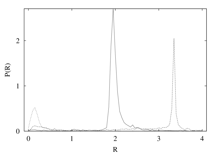
FIG. 3.: As Fig. 2, but for $N=15$.

FIG. 4.: Percentages of ground states with $L=0$ and $L=1$ in the vibron model with random one- and two-body interactions calculated exactly for 100,000 runs (solid lines) and in mean-field approximation (dashed lines).

REFERENCES

- [1] N.V. Zamfir, R.F. Casten and D.S. Brenner, Phys. Rev. Lett. 72, 3480 (1994).
- [2] C.W. Johnson, G.F. Bertsch and D.J. Dean, Phys. Rev. Lett. 80, 2749 (1998).
- [3] R. Bijker, A. Frank and S. Pittel, Phys. Rev. C 60, 021302 (1999).
- [4] C.W. Johnson, G.F. Bertsch, D.J. Dean and I. Talmi, Phys. Rev. C 61, 014311 (2000).
- [5] R. Bijker and A. Frank, Phys. Rev. Lett. 84, 420 (2000).
- [6] R. Bijker and A. Frank, Phys. Rev. C 62, 014303 (2000).
- [7] R. Bijker, A. Frank and S. Pittel, Rev. Mex. Fís. 46 S1, 47 (2000).
- [8] D. Kusnezov, N.V. Zamfir and R.F. Casten, Phys. Rev. Lett. 85, 1396 (2000).
- [9] D. Mulhall, A. Voyla and V. Zelevinsky, Phys. Rev. Lett. 85, 4016 (2000).
- [10] D. Kusnezov, Phys. Rev. Lett. 85, 3773 (2000); R. Bijker and A. Frank, Phys. Rev. Lett 87, 029201 (2001); D. Kusnezov, Phys. Rev. Lett 87, 029202 (2001).
- [11] L. Kaplan, T. Papenbrock and C.W. Johnson, Phys. Rev. 63, 4307 (2001).
- [12] S. Droždž and M. Wójcik, preprint nucl-th/0007045.
- [13] Y.M. Zhao and A. Arima, preprint nucl-th/0108052.
- [14] V. Velázquez and A.P. Zuker, preprint nucl-th/0106020.
- [15] F. Iachello and A. Arima, The interacting boson model (Cambridge University Press, 1987).
- [16] J.N. Ginocchio and M. Kirson, Phys. Rev. Lett. 44, 1744 (1980); A.E.L. Dieperink, O. Scholten and F. Iachello, Phys. Rev. Lett. 44, 1747 (1980).
- [17] J. Dukelsky, G.G. Dussel, R.P.J. Perazzo, S.L. Reich and H.M. Sofia, Nucl. Phys. A 425, 93 (1984).
- [18] P. van Isacker and J.Q. Chen, Phys. Rev. C 24, 684 (1981).
- [19] F. Iachello, Chem. Phys. Lett. 78, 581 (1981).
- [20] F. Iachello, Phys. Rev. C 23, 2778 (1981).
- [21] F. Iachello, N.C. Mukhopadhyay and L. Zhang, Phys. Rev. D 44, 898 (1991).
- [22] O.S. van Roosmalen and A.E.L. Dieperink, Ann. Phys. (N.Y.) 139, 198 (1982); S. Levit and U. Smilansky, Nucl. Phys. A 389, 56 (1982).
- [23] Y.M. Zhao, S. Pittel, R. Bijker, A. Frank and A. Arima, to be published.
- [24] Y. Alhassid, Rev. Mod. Phys. 72, 895 (2000).