Spectral Function of Quarks in Quark Matter

Abstract

We investigate the spectral function of light quarks in infinite quark matter using a simple, albeit self-consistent model. The interactions between the quarks are described by the SU(2) Nambu–Jona-Lasinio model. Currently mean-field effects are neglected and all calculations are performed in the chirally restored phase at zero temperature. Relations between correlation functions and collision rates are used to calculate the spectral function in an iterative process.

I Introduction

It is well known that short-range correlations have influence on the properties of nuclear matter and finite nuclei. The spectral functions observed in $A(e,e^{\prime}p)X$ x1 and $A(e,e^{\prime}pp)X$ x2 experiments are much wider spread than explained by mean-field dynamics. Due to short-range correlations a substantial amount of high-momentum processes is contained in the spectral function.

There have been many theoretical approaches, mainly based on nuclear many-body theory, trying to understand the short-range correlations in nuclei. The results of these calculations have converged in the last years ben ; dick . In particular, the significant population of high-momentum states in the nucleon momentum distribution which is an overall measure for short-range correlations is described rather well.

Our present study is motivated by the work of Lehr et al. le . They have calculated the nucleon spectral function in nuclear matter in a simple model based on transport theory. Direct relations between collision rates and correlation functions form a self-consistency problem and were used to determine the spectral function iteratively. In their calculations the drastic assumption of an averaged, constant scattering amplitude was made. Hence the results are dominated by the properties of the available phase space.

It has turned out that the results of Lehr et al. agree surprisingly well with experimental data cda and sophisticated ”state-of-the-art” calculations from many-body theory ben . Spectral functions, momentum distributions, occupation probabilities, and response functions are all in close agreement with other calculations. It is in particular striking that the only parameter in that model, the coupling strength, is enough to describe size and slope of the high-momentum tail in the nucleon momentum distribution in nuclear matter.

This leads to two conclusions. First, the properties of the nucleon spectral function in nuclear matter are determined by phase space effects and an average strength of the short-range correlations. Second, the detailed structure of the interaction seems to be unimportant as long as the calculations are made in a self-consistent framework.

Due to the success of this model, we take up the concept and make the assumption that similar conditions apply for the short-range correlations in quark matter. Only a few changes to the existing nucleon model are necessary to get a working model for quark matter. First of all, the low current masses of up and down quarks make it necessary to perform the calculations relativistically. This implies some complications since the relativistic, fermionic spectral function is a $4\times 4$ matrix in spinor space. Using symmetry arguments it can be shown that a reduction to three scalar functions is possible. This makes all expressions look more complicated and increases the numerical efforts. However, it does not change the fundamental concept of the model in any way.

In addition a sensible model for the quark interactions has to be used. Our basic assumption is that the details of the interaction should be relatively unimportant as long as the overall strength is correct and the relevant symmetries are respected. Hence we use the well known Nambu–Jona-Lasinio model (NJL model) in its SU(2) version in our calculations. It has the same symmetries as QCD and describes an effective pointlike interaction with a constant coupling strength. Usually the NJL model and its extensions are used in a mean-field approximation. In the spirit of our works on nucleons, we present here an approach that goes beyond the mean-field approximation in a self-consistent way.

In the present work, we use the standard NJL model and do not consider an additional attractive interaction in the quark-quark channel as it appears in extended NJL models that are used in recent works on color superconductivity csc . The aspect of color superconductivity – albeit interesting – is beyond the scope of the present work. A more detailed discussion can be found in sec. II of this paper.

The calculations we present in the following are restricted to the chirally restored phase where the quarks are massless. The relativistic structure of the spectral function gets simpler in this phase, thus simplifying the analytic expressions and reducing the time needed for the numerical calculations significantly. We will come back to that point below.

In sec. II the theoretical aspects of the model are summarized. It is shown how expressions for the self-energy and the spectral function are constructed that are directly related to each other. The resulting self-consistency problem can be solved in an iterative approach. The technical details and the results of our numerical calculations are presented in sec. III. We show the results for the spectral function, its width and the momentum distribution of the quarks. The role of short-range correlations is investigated. Section IV summarizes our results and gives an outlook.

II The Model

II.1 Basic relations

In Ref. le , the model we adopt is described for nonrelativistic nucleons. Many of the details concerning the definition and meaning of the basic quantities can also be found in Refs. kb ; dan . Some aspects of working with relativistic nucleons are discussed in Ref. bo . The fundamental elements of our model are the one-particle Green’s functions without ordering, $g^{>}$ and $g^{<}$. For relativistic fermions they are defined as

$$ig^{>}_{\alpha\beta}(1,1^{\prime}) = \langle\psi_{\alpha}(1)\bar{\psi}_{\beta}(1^{\prime})\rangle$$

$$-ig^{<}_{\alpha\beta}(1,1^{\prime}) = \langle\bar{\psi}_{\beta}(1^{\prime})\psi_{\alpha}(1)\rangle,$$ (1)

where the $\psi$ are field operators in the Heisenberg picture. The indices denote the spin degrees of freedom; isospin and color indices have been supressed here. $1$ and $1^{\prime}$ denote two space-time coordinates. Since we describe fermions with our model the field operators are spinors and the Green’s functions are $4\times 4$ matrices in spinor space.

At this point we also introduce the retarded Green’s function $g^{\mathrm{ret}}$. It is closely related to $g^{\gtrless}$,

$$g^{\mathrm{ret}}_{\alpha\beta}(1,1^{\prime})=\Theta(t_{1}-t_{1^{\prime}})\left[g^{>}_{\alpha\beta}(1,1^{\prime})-g^{<}_{\alpha\beta}(1,1^{\prime})\right].$$ (2)

The Fourier-transformed Green’s functions are used to define the spectral function $\mathcal{A}(p)$. Obviously $\mathcal{A}(p)$ takes over the matrix structure of the Green’s functions

$$\mathcal{A}_{\alpha\beta}(p)=i[g^{>}_{\alpha\beta}(p)-g^{<}_{\alpha\beta}(p)]=-2\mathrm{Im}g^{\mathrm{ret}}_{\alpha\beta}(p),$$ (3)

where ”Im” is given by $\mathrm{Im}F=\frac{1}{2i}(F-\gamma_{0}F^{\dagger}\gamma_{0})$, and correspondingly $\mathrm{Re}F=\frac{1}{2}(F+\gamma_{0}F^{\dagger}\gamma_{0})$.

In addition to eq. (3) the Green’s functions are related to the spectral function via the energy-momentum space distribution function. In thermal equilibrium one has

$$-ig^{<}_{\alpha\beta}(p) = \mathcal{A}_{\alpha\beta}(p)n_{F}(p_{0}),$$ (4)

$$ig^{>}_{\alpha\beta}(p) = \mathcal{A}_{\alpha\beta}(p)[1-n_{F}(p_{0})],$$ (5)

with the thermal Fermi distribution $n_{F}(p_{0})$. At zero temperature the Fermi distribution becomes a step function, $n_{F}(p_{0})=\Theta(\omega_{F}-p_{0})$.

The single particle self-energy of an interacting quantum system can be split into a mean-field part $\Sigma^{\mathrm{mf}}$ and the collisional self-energies $\Sigma^{\gtrless}$. Like the spectral function the self-energy has a matrix structure in spinor space:

$$\Sigma_{\alpha\beta}(1,1^{\prime})=\Sigma^{\mathrm{mf}}_{\alpha\beta}(1,1^{\prime})+\Theta(t_{1}-t_{1^{\prime}})\Sigma^{>}_{\alpha\beta}(1,1^{\prime})+\Theta(t_{1^{\prime}}-t_{1})\Sigma^{<}_{\alpha\beta}(1,1^{\prime}).$$ (6)

The mean-field self-energy is time local, $\Sigma^{\mathrm{mf}}\sim\delta(t_{1}-t_{1^{\prime}})$. It describes the effects corresponding to the motion of noninteracting particles in a mean-field potential and is responsible for the dynamical generation of the constituent quark masses. The collisional part of the self-energy contains the effects that arise from decays and particle collisions in the medium.

As for the Green’s functions a retarded self-energy is introduced

$$\Sigma^{\mathrm{ret}}_{\alpha\beta}(1,1^{\prime})=\Sigma^{\mathrm{mf}}_{\alpha\beta}(1,1^{\prime})+\Theta(t_{1}-t_{1^{\prime}})\left[\Sigma^{>}_{\alpha\beta}(1,1^{\prime})-\Sigma^{<}_{\alpha\beta}(1,1^{\prime})\right].$$ (7)

In momentum space the width of the spectral function is given by the imaginary part of this retarded self-energy. One has

$$\Gamma_{\alpha\beta}(p)=-2\mathrm{Im}\Sigma^{\mathrm{ret}}_{\alpha\beta}(p)=i[\Sigma^{>}_{\alpha\beta}(p)-\Sigma^{<}_{\alpha\beta}(p)].$$ (8)

$\Sigma^{\mathrm{mf}}$ does not contribute to the imaginary part of $\Sigma^{\mathrm{ret}}(p)$ since it is time local. Hence the width of the spectral function is completely given by the collisional self-energies $\Sigma^{\gtrless}$. In kb it has been shown that $i\Sigma^{>}(p)$ and $-i\Sigma^{<}(p)$ are identical to the total collision rates for scattering into (gain rate) and out of (loss rate) the configuration $(p_{0},\vec{p})$, respectively.

From analyticity it follows that the real part of the self-energy is related to $\Gamma$ by a dispersion relation

$$\mathrm{Re}\Sigma^{\mathrm{ret}}(p)=\Sigma^{\mathrm{mf}}(p)+\mathcal{P}\int\frac{dp_{0}^{\prime}}{2\pi}\frac{\Gamma(p_{0}^{\prime},\vec{p})}{p_{0}-p_{0}^{\prime}}.$$ (9)

If the width is known over the full energy range the real part of $\Sigma^{\mathrm{ret}}$ can be calculated dispersively.

II.2 Interactions in the NJL Model

In the following, we use the standard SU(2) version of the NJL model klev ; klvw . It has been designed to resemble the symmetries of QCD. In particular, it allows the dynamical generation of fermion masses via the mechanism of chiral symmetry breaking. The Lagrangian of this effective interaction is given by

$$\mathcal{L}_{\mathrm{NJL}}=\bar{\psi}i\partial\!\!\!/\psi+G[(\bar{\psi}\psi)^{2}+(\bar{\psi}i\gamma_{5}\vec{\tau}\psi)^{2}],$$ (10)

where $G$ is the coupling strength, independent of energy and momentum, and the $\tau_{i}$ are the isospin Pauli matrices. The small current quark masses are neglected here.

The pointlike interaction renders this model nonrenormalizable. In our calculations we deal with this problem by introducing a cutoff for the three-momenta. This cutoff and the coupling constant are the free parameters of the NJL model. Usually their values are chosen so that the model reproduces the correct values for the quark condensate and the pion decay constant in vacuum.

Before we continue with the discussion of our present model we want to comment on its relation to other present investigations. Recent works on color superconductivity csc ; berg ; lang consider an extended NJL model. In the case of two flavors the interaction is given by

$$\mathcal{L}_{\mathrm{int}}=G_{1}[(\bar{\psi}\psi)^{2}+(\bar{\psi}i\gamma_{5}\vec{\tau}\psi)^{2}]+G_{2}(\bar{\psi}i\gamma_{5}\tau_{2}\lambda_{2}\bar{\psi}^{T})(\psi^{T}Ci\gamma_{5}\tau_{2}\lambda_{2}\psi),$$ (11)

where $C$ is the charge conjugation operator and $\lambda_{2}$ is a Gell-Mann matrix in color space. $G_{1}$ and $G_{2}$ are coupling constants. In the mean-field approximation, the new term on the right of eq. (11) introduces an attractive interaction in the quark-quark channel that can lead to a pairing of quarks at the Fermi surface. This pairing breaks the color symmetry spontaneously and gives rise to color superconductivity. We note in the passing that the use of such an extended Lagrangian is not free from ambiguities berg ; lang due to the freedom of Fierz rearrangements.

As we will discuss below, we go beyond the mean-field approximation in our approach. We have decided as a first step to construct a consistent model based on the well established Lagrangian (10). An additional attractive quark-quark channel is not considered at this stage. Color superconductivity is definitely an interesting phenomenon and can be incorporated into the model in the future.

II.3 Structure of the relativistic expressions

As shown above the spectral function of relativistic fermions has a matrix structure. The most general form of this structure is found by writing the spectral function in terms of the 16 linear independent products of the $\gamma$ matrices (Clifford algebra) and demanding the invariance under certain symmetries bd . We consider here parity and time-reversal symmetry. A strongly interacting system of infinite size and in thermal equilibrium is invariant under these transformations. In the rest frame of the medium this leads to the following form for the spectral function:

$$\mathcal{A}(p)=\rho_{\mathrm{s}}(p_{0},\vec{p}^{\,2})+\rho_{\mathrm{0}}(p_{0},\vec{p}^{\,2})\cdot\gamma^{0}+\rho_{\mathrm{v}}(p_{0},\vec{p}^{\,2})\hat{\vec{p}}\cdot\vec{\gamma},$$ (12)

where $\hat{\vec{p}}$ is a unit vector in the momentum direction. As a first step we restrict our calculations in the present work to the chirally restored phase. Since the ”scalar” term $\rho_{\mathrm{s}}$ is not chirally invariant it has to be zero; the spectral function is then completely determined by the two scalar functions $\rho_{0}$ and $\rho_{\mathrm{v}}$. Note that the spectral function for free quarks with $p_{0}>0$ is given by $\mathcal{A}=\pi|\vec{p}|^{-1}\!\not\!p\,\delta(p_{0}-|\vec{p}|)$. According to our choice of signs in eq. (12) this means that $\rho_{0}>0$ and $\rho_{\mathrm{v}}<0$ in this case.

The structure of the self-energies $\Sigma^{\gtrless}$ and the width $\Gamma$ are identical to that of the spectral function. They too consist of three scalar functions,

$$\Sigma^{\gtrless}(p) = \Sigma^{\gtrless}_{\mathrm{s}}(p_{0},\vec{p}^{\,2})+\Sigma^{\gtrless}_{\mathrm{0}}(p_{0},\vec{p}^{\,2})\cdot\gamma^{0}+\Sigma^{\gtrless}_{\mathrm{v}}(p_{0},\vec{p}^{\,2})\hat{\vec{p}}\cdot\vec{\gamma},$$ (13)

$$\Gamma(p) = \Gamma_{\mathrm{s}}(p_{0},\vec{p}^{\,2})+\Gamma_{\mathrm{0}}(p_{0},\vec{p}^{\,2})\cdot\gamma^{0}+\Gamma_{\mathrm{v}}(p_{0},\vec{p}^{\,2})\hat{\vec{p}}\cdot\vec{\gamma},$$ (14)

with $\Sigma^{\gtrless}_{\mathrm{s}}=\Gamma_{\mathrm{s}}=0$ in the chirally symmetric phase.

II.4 Self-consistent expressions

The mean-field part $\Sigma^{\mathrm{mf}}$ of the self-energy is given by the tadpole diagrams. Currently chiral symmetry is restored ”by hand” in our model. This means that the system under consideration is forced into the chirally restored phase by setting the constituent quark masses, i.e., the Hartree term of $\Sigma^{\mathrm{mf}}$ to zero. The Fock term contains a part that needs not to be zero but this part can be absorbed in a redefinition of the chemical potential klev . Note that one can do this for any temperature and chemical potential since the gap equation for the quark masses klev ; klvw is always solved for $m=0$. However, thermodynamically this might not be the favored phase when there exists also a finite solution for the gap equation.

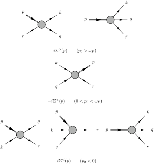
Figure 2: Scattering processes corresponding to the self-energies $\Sigma^{\gtrless}(p)$ in the Born approximation. The double lines carry the four-momentum $p$ of $\Sigma^{\gtrless}$; $p,q,k,r$ denote quarks with four-momentum $(p_{0},\vec{p})$, etc. (with $p_{0},q_{0},k_{0},r_{0}>0$), and $\bar{p},\bar{q},\bar{k},\bar{r}$ denote antiquarks with four-momentum $(-p_{0},\vec{p})$, etc. (with $p_{0},q_{0},k_{0},r_{0}<0$). Total collision rates are found by integrating over the four-momenta $k,q,r$ (respectively $\bar{k},\bar{q},\bar{r}$), i.e., all lines except the double line. In the first row the scattering-out processes contributing to the loss rate $i\Sigma^{>}$ are shown. The second row shows the only contribution to the gain rate $-i\Sigma^{<}$ for positive $p_{0}$. In the last row the processes contributing to the antiparticle loss rate $-i\Sigma^{<}$ at $p_{0}<0$ are shown. Note that there are no contributions to $\Sigma^{>}$ for $p_{0}<\omega_{F}$ and to $\Sigma^{<}$ for $p_{0}>\omega_{F}$ at zero temperature.

The collisional self-energies $\Sigma^{\gtrless}$ can be calculated diagrammatically. We restrict ourselves to the lowest order, given by the direct and the exchange Born diagram (see Fig. 1). In this approximation only two particle correlations are included in the model. The corresponding processes at finite chemical potential (cf. Ref. kb ) are shown in Fig. 2.

In perturbation theory the particle and antiparticle lines in the diagrams of Fig. 1 are interpreted as free propagators. Our model, however, takes into account the in-medium character of the intermediate states. The lines are interpreted as full relativistic Green’s functions which again depend on the self-energies via the spectral function (eqs. (4) and (5)). This way we end up with self-consistent expressions for the self-energies. In the language of Feynman diagrams the use of full Green’s functions means that we sum over a whole class of diagrams. Note that no ambiguities concerning Fierz rearrangements appear here. All interactions at the two loop level caused by the interaction term in eq. (10) are included in our approach. In particular, we find contributions from quark-quark as well as from quark-antiquark scattering (cf. Fig. 2).

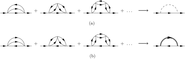
Figure 4: Series of diagrams that correspond to the coupling of dynamically generated mesons (a) and diquarks (b) to the quarks (see klev ; klvw for details). The dashed line is a pion or sigma and the dotted line is a diquark. In the present model only the lowest order diagram, the sunset diagram, is included.

At this point it might be illuminating to discuss which Feynman diagrams are resummed by our approach and which ones are not. We use full propagators for the calculation of the sunset diagram depicted in Fig. 1. In this way we include diagrams like the ones shown in Fig. 3. We do not sum up the series shown in Fig. 4 (a) (we only have the first term). Series of that type would correspond to the coupling of dynamically generated pions or sigmas to the quarks klev ; klvw . Clearly such series are relevant in the chirally broken phase. We also do not sum up the series shown in Fig. 4 (b), which corresponds to coupling to diquarks. This is expected to be relevant if the phenomenon of color superconductivity is tackled.

Working out the diagrams and replacing the Green’s functions $g^{\gtrless}$ by spectral functions according to eqs. (4) and (5) one gets for the two components of $i\Sigma^{>}(p)$ in the chirally restored phase

$$i\Sigma^{>}_{0}(p) = \frac{G^{2}}{(2\pi)^{6}}\int dk_{0}dq_{0}\int_{<\Lambda}du^{2}dv^{2}\int d\cos\vartheta_{uv}[1-n_{F}(k_{0})]uv$$ (15)

$$\Bigg{\{}14\left[\left(\rho_{0}(k)\rho_{0}(q)-\rho_{\mathrm{v}}(q)\rho_{\mathrm{v}}(k)\frac{u^{2}-v^{2}}{|\vec{u}+\vec{v}||\vec{u}-\vec{v}|}\right)n_{F}(q_{0})[1-n_{F}(r_{0})]\right.$$

$$\left.\times\frac{1}{2|\vec{p}|v}\int^{\vec{p}^{\,2}+v^{2}+2|\vec{p}|v}_{\vec{p}^{\,2}+v^{2}-2|\vec{p}|v}dr^{2}\rho_{0}(r_{0},r^{2})\right]_{{\vec{k}=\frac{1}{2}(\vec{u}-\vec{v})\atop\vec{q}=\frac{1}{2}(\vec{u}+\vec{v})}\atop r_{0}=p_{0}+q_{0}-k_{0}}$$

$$-\left[\left(\rho_{0}(k)\rho_{0}(q)-\rho_{\mathrm{v}}(q)\rho_{\mathrm{v}}(k)\frac{u^{2}-v^{2}}{|\vec{u}+\vec{v}||\vec{u}-\vec{v}|}\right)[1-n_{F}(q_{0})]n_{F}(r_{0})\right.$$

$$\left.\times\frac{1}{2|\vec{p}|u}\int^{\vec{p}^{\,2}+u^{2}+2|\vec{p}|u}_{\vec{p}^{\,2}+u^{2}-2|\vec{p}|u}dr^{2}\rho_{0}(r_{0},r^{2})\right]_{{\vec{k}=\frac{1}{2}(\vec{u}-\vec{v})\atop\vec{q}=\frac{1}{2}(\vec{u}+\vec{v})}\atop r_{0}=q_{0}+k_{0}-p_{0}}\Bigg{\}}$$

and

$$i\Sigma^{>}_{\mathrm{v}}(p) = \frac{G^{2}}{(2\pi)^{6}}\int dk_{0}dq_{0}\int_{<\Lambda}du^{2}dv^{2}\int d\cos\vartheta_{uv}[1-n_{F}(k_{0})]uv$$

$$\Bigg{\{}14\left[\left(\rho_{0}(k)\rho_{0}(q)-\rho_{\mathrm{v}}(q)\rho_{\mathrm{v}}(k)\frac{u^{2}-v^{2}}{|\vec{u}+\vec{v}||\vec{u}-\vec{v}|}\right)n_{F}(q_{0})[1-n_{F}(r_{0})]\right.$$

$$\left.\times\frac{1}{4|\vec{p}|v}\int^{\vec{p}^{\,2}+v^{2}+2|\vec{p}|v}_{\vec{p}^{\,2}+v^{2}-2|\vec{p}|v}dr^{2}\rho_{\mathrm{v}}(r_{0},r^{2})\frac{1}{r}\left(\frac{r^{2}-v^{2}}{\vec{p}^{2}}+1\right)\right]_{{\vec{k}=\frac{1}{2}(\vec{u}-\vec{v})\atop\vec{q}=\frac{1}{2}(\vec{u}+\vec{v})}\atop r_{0}=p_{0}+q_{0}-k_{0}}$$

$$+\left[\left(\rho_{0}(k)\rho_{0}(q)-\rho_{\mathrm{v}}(q)\rho_{\mathrm{v}}(k)\frac{u^{2}-v^{2}}{|\vec{u}+\vec{v}||\vec{u}-\vec{v}|}\right)[1-n_{F}(q_{0})]n_{F}(r_{0})\right.$$

$$\left.\times\frac{1}{4|\vec{p}|u}\int^{\vec{p}^{\,2}+u^{2}+2|\vec{p}|u}_{\vec{p}^{\,2}+u^{2}-2|\vec{p}|u}dr^{2}\rho_{\mathrm{v}}(r_{0},r^{2})\frac{1}{r}\left(\frac{r^{2}-u^{2}}{\vec{p}^{2}}+1\right)\right]_{{\vec{k}=\frac{1}{2}(\vec{u}-\vec{v})\atop\vec{q}=\frac{1}{2}(\vec{u}+\vec{v})}\atop r_{0}=q_{0}+k_{0}-p_{0}}\Bigg{\}}.$$

Here $\vec{u}=\vec{q}+\vec{k}$ and $\vec{v}=\vec{q}-\vec{k}$ are the center of mass and relative momenta in the scattering processes of Fig. 2. $\vartheta_{uv}$ is the angle between the two vectors $\vec{u}$ and $\vec{v}$. The subscript ”$<\Lambda$” at the integrals indicates that a three-momentum cutoff is applied. This notation requires some comments: The integrals in eqs. (15) and (II.4) are integrals for $\vec{u}$ and $\vec{v}$. In practice, however, the cutoff is applied to $\vec{k}$ and $\vec{q}$ in the calculations. The vectors $\vec{k}$ and $\vec{q}$ are the momenta of the particles and antiparticles in Fig. 1, thus they must be regularized when working out the diagrams.

The expressions for $-i\Sigma^{<}_{0}(p)$ and $-i\Sigma^{<}_{\mathrm{v}}(p)$ are not presented here. They are easily found from eqs. (15) and (II.4) by replacing all functions $n_{F}$ by $(1-n_{F})$ and vice versa.

Eqs. (15) and (II.4) relate the collisional self-energies (collision rates) to the spectral function. Note that the zeroth and the vector component of eq. (12) are mixed. Finally, the components of the spectral function have to be expressed in terms of the self-energies $\Sigma^{\gtrless}$ via the width $\Gamma$. The expressions are found by inserting the explicit form of the relativistic in-medium Green’s function,

$$g^{\mathrm{ret}}(p)=\frac{1}{\not\!p-\Sigma^{\mathrm{ret}}(p)},$$ (17)

into the definition of the spectral function (3). Since the chirally restored phase is considered the quarks are massless and no mass term appears in the denominator.

When working out the imaginary part of $g^{\mathrm{ret}}$ one also needs the real part of the self-energy $\Sigma^{\mathrm{ret}}$. In principle it can be calculated from $\Gamma$ by use of the dispersion relation (9). The studies of Lehr et al. le have shown that the influence of $\mathrm{Re}\Sigma^{\mathrm{ret}}$ on the nucleon spectral function and the nucleon momentum distribution in nuclear matter is small. In their first calculations they have replaced $\mathrm{Re}\Sigma^{\mathrm{ret}}(p)$ by a constant value independent of energy and momentum. It was found that this violation of analyticity leads only to minor effects in the results.

In our present calculations, we are not able to use the dispersion relation (9) due to technical reasons. We work on a finite grid in energy and momentum space, the boundaries of which have been chosen to include all significant parts of the spectral function. The width $\Gamma_{0}$, however, extends much further into the high energy regions than the spectral function. As we do not know $\Gamma_{0}$ outside the grid, the $p_{0}$ integration of the dispersion integral cannot be performed.

In principle, one could find $\mathrm{Re}\Sigma^{\mathrm{ret}}$ in a different way. Using the dispersion relation for the retarded propagator, $\mathrm{Re}g^{\mathrm{ret}}$ can be calculated from the spectral function. Then it is possible to deduce $\mathrm{Re}\Sigma^{\mathrm{ret}}$ from eq. (17). We have checked this and it turned out that the real part of the self-energy is very small compared to $p_{0}$ and $|\vec{p}|$, i.e., in $\not\!p-\mathrm{Re}\Sigma^{\mathrm{ret}}$ the dominant part is $\not\!p$. Since we know from the nucleons that the real part of $\Sigma^{\mathrm{ret}}$ is relatively unimportant $\mathrm{Re}\Sigma^{\mathrm{ret}}$ is set to zero in the following.

The following expressions for $\rho_{0}$ and $\rho_{\mathrm{v}}$ are found from eqs. (3) and (17), when $\mathrm{Re}\Sigma^{\mathrm{ret}}$ is set to zero

$$\rho_{0}(p_{0},\vec{p}^{\,2}) = \frac{(p_{0}^{2}+\vec{p}^{\,2})\Gamma_{0}+\frac{1}{4}(\Gamma_{0}^{2}-\Gamma_{\mathrm{v}}^{2})\Gamma_{0}+2p_{0}|\vec{p}|\Gamma_{\mathrm{v}}}{[p_{0}^{2}-\vec{p}^{\,2}-\frac{1}{4}\Gamma_{0}^{2}+\frac{1}{4}\Gamma_{\mathrm{v}}^{2}]^{2}+[p_{0}\Gamma_{0}-\Gamma_{\mathrm{v}}|\vec{p}|]^{2}},$$ (18)

$$\rho_{\mathrm{v}}(p_{0},\vec{p}^{\,2}) = -\frac{(p_{0}^{2}+\vec{p}^{2})\Gamma_{\mathrm{v}}-\frac{1}{4}(\Gamma_{0}^{2}-\Gamma_{\mathrm{v}}^{2})\Gamma_{\mathrm{v}}+2p_{0}|\vec{p}|\Gamma_{0}}{[p_{0}^{2}-\vec{p}^{\,2}-\frac{1}{4}\Gamma_{0}^{2}+\frac{1}{4}\Gamma_{\mathrm{v}}^{2}]^{2}+[p_{0}\Gamma_{0}-\Gamma_{\mathrm{v}}|\vec{p}|]^{2}}.$$ (19)

The two relations look very similar. Up to some signs only $\Gamma_{0}$ and $\Gamma_{\mathrm{v}}$ are exchanged in the numerator. Near the on-shell point $\rho_{0}$ and $\rho_{\mathrm{v}}$ differ only by a minus sign at positive $p_{0}$ if terms $\sim\mathcal{O}(\Gamma^{3})$ are neglected

$$\rho_{0}(p_{0},p_{0}^{2})\approx\frac{2p_{0}^{2}\Gamma_{0}+2p_{0}|p_{0}|\Gamma_{\mathrm{v}}}{\cdots}~{},\qquad\rho_{\mathrm{v}}(p_{0},p_{0}^{2})\approx-\frac{2p_{0}^{2}\Gamma_{\mathrm{v}}+2p_{0}|p_{0}|\Gamma_{0}}{\cdots}.$$ (20)

Eqs. (15) and (II.4), (18) and (19), and eq. (8) form a set of equations describing a self-consistency problem. A direct solution of this problem is not possible but the equations can be used to calculate the spectral function iteratively.

III Numerics and results

III.1 Details of the calculation

All calculations were performed at zero temperature in the chirally restored phase. We have used two different quark densities. Motivated from the investigations for nucleons in nuclear matter, we chose the quark matter in the first case such that it is comparable to regular nuclear matter. As every nucleon consists of three valence quarks the quark density was set to $\rho_{\mathrm{qm}}=3\cdot\rho_{\mathrm{nm}}=3\cdot 0.17\,\mathrm{fm}^{-3}$. For the number of flavors we use $N_{\mathrm{f}}=2$ (up and down). This yields a Fermi energy and a Fermi momentum of $\omega_{F}=p_{F}=0.268\,\mathrm{GeV}$ for massless quarks. In reality quark matter with that chemical potential would not be in the chirally restored phase. Therefore, we have also worked with a three times higher density, $\rho_{\mathrm{qm}}=1.53\,\mathrm{fm}^{-3}$, corresponding to a Fermi energy of $\omega_{F}=0.387\,\mathrm{GeV}$. This case seems to be more realistic for chirally symmetric quark matter, the chemical potential is well beyond the chiral phase transition in the NJL model klev ; klvw . Note that all states at energies up to $\omega_{F}$ are filled. This includes the states at negative energies. Thus there are no holes in the Dirac sea which could be identified with populated antiquark states.

The three-momentum cutoff $\Lambda=653\,\mathrm{MeV}$ and the coupling constant $G=2.14\cdot\Lambda^{-2}$ of the NJL model were chosen so that the model gives the known values for the quark condensate, $\langle\bar{u}u\rangle=\langle\bar{d}d\rangle=-(250\,\mathrm{MeV})^{3}$, and the pion coupling constant, $f_{\pi}=93\,\mathrm{MeV}$, in vacuum klev . In the case of the lower density we performed also calculations with two times and four times larger coupling strengths to investigate the influence on the spectral function.

The calculations were carried out on an energy-momentum grid with boundaries $-653\,\mathrm{MeV}\leq p_{0}\leq 653\,\mathrm{MeV}$ and $|\vec{p}|\leq 653\,\mathrm{MeV}$ (in correspondence to the NJL cutoff) and a mesh size of $6.53\,\mathrm{MeV}$ in both directions. Due to the cutoff a grid of that size is sufficient to include all significant parts of the spectral function. The states with negative energies $p_{0}$ are interpreted as anti-quark states with positive energies $|p_{0}|$ in the discussion of the results.

To initialize the calculations a constant width, $\Gamma_{0}=1\,\mathrm{MeV}$ and $\Gamma_{\mathrm{v}}=0$, was used. In principle it would be interesting to start from a quasiparticle approximation with a width much smaller than the final result. This would allow to observe the redistribution of strength away from the peaks during the iterations. However, this is numerically not feasible. So the initialization values are not too far away from the final results and only two iterations were necessary to reach self-consistency.

III.2 Results

In this section, we present the results of our iterative calculations. Before the spectral function is discussed we have a look at the width $\Gamma$. This is helpful to understand the resulting spectral functions and it allows a clearer observation of the iterative process than the spectral function itself.

We show the results for $\rho_{0}$ and $\Gamma_{0}$ but not for $\rho_{\mathrm{v}}$ and $\Gamma_{\mathrm{v}}$. Most of the interesting structure of the spectral function is located around the on-shell peaks. It has been discussed that $\rho_{0}$ and $\rho_{\mathrm{v}}$ differ at most by a sign near those peaks (eq. (20)). Thus it is not surprising that both look very similar and it is sufficient to show only one of them. The reason to show $\rho_{0}$ is that the density of states (particles minus antiparticles) is given by $\rho_{0}$ alone,

$$\mathrm{Tr}\{\gamma_{0}\mathcal{A}(p)\}=4\cdot N_{\mathrm{f}}N_{\mathrm{c}}\rho_{0}(p_{0},\vec{p}^{\,2}).$$ (21)

There is no simple relation between $\Gamma_{0}$ and $\Gamma_{\mathrm{v}}$ justifying to show only one. But our results show that $\Gamma_{\mathrm{v}}$ is much smaller than $\Gamma_{0}$ (this has also been observed in calculations for relativistic nucleons horo ). Hence $\Gamma_{\mathrm{v}}$ seems rather uninteresting since its influence on the spectral function is minimal.

Figure 5 shows cuts of the width $\Gamma_{0}$ at several momenta for $\omega_{F}=0.268\,\mathrm{GeV}$. The dotted line is the result after the first iteration while the solid line displays the final, self-consistent result. Physically the most interesting area lies in the energy range $0<p_{0}<\omega_{F}$ since that is the location of the populated quark states. All states above the Fermi energy as well as the antiquark states at negative $p_{0}$ are unoccupied (no holes in the Dirac sea). $\Gamma_{0}$ takes on low values of $0.1-1\,\mathrm{MeV}$ in this zone, being close to the initialization value.

The two most important features of $\Gamma_{0}$ are clearly visible. First, the width is zero along the Fermi energy $\omega_{F}$, the quarks along this line are quasiparticles. Due to Pauli blocking and energy conservation it is not possible to scatter into or out of this configurations at zero temperature. Second, the width grows explosively at high $|p_{0}|$. The reason for this is the pointlike interaction of the NJL model. The self-energies $\Sigma^{\gtrless}$ essentially sum up the phase space available for scattering processes. The opening of this phase space at large $|p_{0}|$ can be directly read off from $\Gamma_{0}$. The three-momentum cutoff applied in the calculations stops this inflational behavior at higher energies. These energies, however, are outside of our grid. A simple (on-shell) estimate shows that the maximum width is reached at $\Lambda<|p_{0}|<2\Lambda$ and that the width must be zero for $|p_{0}|>3\Lambda$ .

Another noticeable feature is the local minimum in the antiparticle sector, most visible at low momenta. This is a phase space effect that can be easily explained by the energy and momentum dependence of the particle correlations. In the bottom row of Fig. 2 all processes contributing to the width at negative $p_{0}$ are shown. Phase space opens for the processes $\bar{p}k\rightarrow\bar{q}r$ and $\bar{p}\rightarrow\bar{k}\bar{q}r$ at $p_{0}=0$ and $p_{0}=-\omega_{F}$, respectively, and grows with decreasing $p_{0}$. On the other hand the process $\bar{p}kq\rightarrow r$ is possible for $p_{0}>-|\vec{p}|$ only. Its phase space grows with increasing $p_{0}$ and is maximal at $p_{0}=0$. The overlap of these three processes leads to the observed minimum that is situated approximatly at $p_{0}=-|\vec{p}|$ for low momenta.

In Fig. 6, the width $\Gamma_{0}$ is shown for $\omega_{F}=0.268\,\mathrm{GeV}$ at several values for the coupling strength; all curves are self-consistent final results. The solid lines show the result at the original coupling of $G=2.14\cdot\Lambda^{-2}$, the dashed lines were obtained for $G=2\cdot 2.14\cdot\Lambda^{-2}$ and the dotted lines display the width at a coupling strength of $G=4\cdot 2.14\cdot\Lambda^{-2}$. The larger couplings lead to a significant increase of the width. Since $G$ enters the self-energies as a factor of $G^{2}$ it is not surprising that a two times larger coupling results in a four times larger width and a four times larger coupling causes a width 16 times larger. The shape of $\Gamma_{0}$ does not change very much. Only the gap in the antiquark sector gets smeared out due to the increased width which weakens the restrictions for the scattering processes.

Figure 7 displays $\Gamma_{0}$ for the different chemical potentials $\omega_{F}=0.268\,\mathrm{GeV}$ and $\omega_{F}=0.387\,\mathrm{GeV}$ at the regular coupling strength. The higher chemical potential has a similar effect as an increased coupling. Essentially, a scaling of the width can be observed while the general shape of $\Gamma_{0}$ remains unaffected. For $p_{0}>\omega_{F}$ one would expect a width $\Gamma_{0}\sim\rho$. This is, however, hard to see because of the vicinity to the cutoff in our calculations. For $p_{0}<\omega_{F}$, i.e., for the hole width, one expects a width $\Gamma_{0}\sim\rho^{2}$ (see Fig. 2, second line), because both momenta $k$ and $q$ lie within the Fermi sea. The observed scaling, however, is slightly smaller. This is due to the fact that the cutoff suppresses outgoing states with energies $r_{0}>\Lambda$ that can be reached when $\omega_{F}>\Lambda/2$. So the widths in our results differ not by a factor of $9$ but only by a factor of $\sim 6$ as one would expect for a Fermi energy of $\omega_{F}=\Lambda/2$ (this is the largest Fermi energy possible for which no outgoing states are suppressed).

The spectral function defines the spectrum of possible energies $p_{0}$ for a particle or antiparticle with momentum $\vec{p}$ that is added to the medium. In Fig. 8, $\rho_{0}$ is shown for the three coupling strengths at the lower chemical potential of $\omega_{F}=0.268\,\mathrm{GeV}$. The structure is clearly dominated by the two peaks at $p_{0}=|\vec{p}|$ and $p_{0}=-|\vec{p}|$. These are the on-shell peaks of the quarks and the antiquarks. Because of the small widths they are very narrow and most of the strength is concentrated there. As one would expect from the results for $\Gamma_{0}$ the peaks get broader and less high when the coupling is increased. Thus strength is removed from the peaks to the off-shell regions. The background of the spectral function seems to scale with the coupling in a similar way as $\Gamma_{0}$. Approximately a quadratic dependence is found.

The spectral function for the quarks and the antiquarks is not symmetric. This is due to the finite chemical potential: The quarks of our medium fill up all states up to the Fermi energy. Due to Pauli blocking only scattering processes with outgoing quarks at energies above $\omega_{F}$ are allowed. Incoming quarks from the medium must always have energies below $\omega_{F}$. On the other hand, all antiquark states are empty. Scattering processes with outgoing antiquarks at all energies are possible. However, there are no processes with incoming antiquarks from the medium.

Since we are interested in short-range correlations the spectral function at large momenta above the Fermi momentum is of particular interest. The cut at $|\vec{p}|=0.3\,\mathrm{GeV}$ in Fig. 8 indicates that short-range correlations seem rather weak for the original coupling strength, the spectral function is very small at $0<p_{0}<\omega_{F}$. Only when the coupling is increased a significant population of high momentum states can be observed.

In Fig. 9, the influence of the chemical potential on the spectral function is illustrated. As expected from the results for the width the peaks get broader and less high for the larger chemical potential of $\omega_{F}=0.387\,\mathrm{GeV}$. Of particular interest is the cut for $|\vec{p}|=0.5\,\mathrm{GeV}$ (i.e., $p>p_{F}$). A bump in the region of the occupied quark states indicates the growing importance of short-range correlations for higher $\omega_{F}$ (one should compare this bump to the cuts for $|\vec{p}|=0.3\,\mathrm{GeV}$ in Fig. 8 to take into account the different Fermi momenta).

Finally we take a look at the (normalized) momentum distribution of the quarks which is given by

$$n(|\vec{p}|)=\int_{0}^{\omega_{F}}\frac{dp_{0}}{\pi}\rho_{0}(p_{0},|\vec{p}|).$$ (22)

The momentum distribution of nucleons in nuclear matter or nuclei shows a depletion of occupation probabilites by about 10% le . The resulting high-momentum tail is taken as a universal sign of short-range correlations. Figure 10 displays the quark momentum distribution at the different coupling strengths for $\omega_{F}=0.268\,\mathrm{GeV}$. As expected for an infinite system a sharp step at the Fermi momentum appears. At the lowest coupling a depletion of only 0.1% is found. This confirms the previous interpretation of the spectral function. For the coupling twice as large the short-range correlations increase but still the depletion effect is below 1%. Only for the largest couplings we find a high-momentum tail of a few percent, comparable to the case of nucleons. Figure 11 shows again that the larger chemical potential has an effect similar to the increased couplings. The depletion for $\omega_{F}=0.387\,\mathrm{GeV}$ grows by almost one order of magnitude compared to the case of $\omega_{F}=0.268\,\mathrm{GeV}$ and the original coupling strength. It has a size of almost 1% and is comparable to the result for the two times larger coupling.

IV Summary and conclusions

In this paper we have presented an approach to the spectral function of quarks in quark matter. Based on a successful concept for nuclear matter it was shown how to construct a simple model for the quarks. Using the relations between collisional self-energies and the spectral function an iterative method was derived that goes beyond the quasiparticle approximation. Assuming that the exact structure of the interaction is irrelevant for the calculations – an important finding for nuclear matter – the pointlike interaction of the NJL model was used in the calculations.

Our calculations, which are currently restricted to zero temperature and the chirally restored phase, show that we are able to deal with the numerical difficulties implied by this approach. However, the results also indicate that the influence of short-range correlations is small compared to nuclear matter. This finding, however, might be an artefact of the present model, the NJL model with vacuum parameters in the Born approximation. Since we know now that the model is technically feasible we can go beyond the simple model presented here. It is our plan to use more sophisticated interaction models for future calculations and to explore also other phases with broken symmetries.

Figure 1: Lowest order contributions to the self-energy $i\Sigma^{>}(p)$ in the SU(2) NJL model (Born diagrams). Since we have a pointlike interaction the direct and the exchange diagrams look the same in this figure.

Figure 3: Examples for diagrams that are resummed in our self-consistent calculation. In this figure the lines correspond to free propagators. Once the elementary sunset diagram on the left is constructed from full propagators the other diagrams are automatically resummed.

Figure 5: Width of the spectral function of quarks at different momenta. The dashed line shows the result after the first iteration, the solid line shows the final result after two iterations.

Figure 6: Width of the spectral function of quarks at different momenta. The solid line shows the width at the usual coupling strength ($G=2.14\cdot\Lambda^{-2}$), the dashed line is the result at a coupling twice as large and the dotted line has been obtained with a coupling four times larger than the usual value.

Figure 7: Width of the spectral function at two different momenta. The solid line shows the result at a chemical potential of $\omega_{F}=0.387\,\mathrm{GeV}$ while the dashed line has been found for $\omega_{F}=0.268\,\mathrm{GeV}$ (cf. Fig. 6). In both cases a coupling of $G=2.14\cdot\Lambda^{-2}$ has been used.

Figure 8: The spectral function of quarks at different momenta and couplings (cf. Fig. 6 for details).

Figure 9: The spectral function for two different chemical potentials and momenta (see Fig. 7 for details).

Figure 10: Quark momentum distribution in quark matter at different coupling strengths (see Fig. 6 for details).

Figure 11: Quark momentum distribution in quark matter for two different chemical potentials (see Fig. 7 for details).

References

- (1) For a review see, e.g., P.K.A. de Witt Huberts, J. Phys. G (Nucl. Part. Phys.) 16, 507 (1990).
- (2) G. Rosner, in Perspectives in Hadronic Physics edited by S. Boffi, C. Ciofi degli Atti, and M.M. Giannini (World Scientific, Singapore, 1998).
- (3) O. Benhar, A. Fabrocini, S. Fantoni, Nucl. Phys. A505, 267 (1989); O. Benhar, A. Fabrocini, S. Fantoni, Nucl. Phys. A550, 201 (1992).
- (4) A. Ramos, A. Polls, and W.H. Dickhoff, Nucl. Phys. A503, 1 (1990); A. Ramos, A. Polls, and W.H. Dickhoff, Phys. Rev. C 43, 2239 (1991).
- (5) J. Lehr, M. Effenberger, H. Lenske, S. Leupold, U. Mosel, Phys. Lett. B 483, 324 (2000); J. Lehr, H. Lenske, S. Leupold, U. Mosel, Nucl. Phys. A703, 393 (2002).
- (6) C. Ciofi degli Atti, E. Pace, G. Salme, Phys. Rev. C 43, 1155 (1991).
- (7) See, e.g., R. Rapp, T. Schäfer, E.V. Shuryak, M. Velkovsky, Phys. Rev. Lett. 81, 53 (1998); M.G. Alford, K. Rajagopal, F. Wilczek, Phys. Lett. B 422, 247 (1998); G.W. Carter, D. Diakonov, Phys. Rev. D 60, 016004 (1999); T.M. Schwarz, S.P. Klevansky, G. Papp, Phys. Rev. C 60, 055205 (1999); M. Buballa, M. Oertel, Nucl. Phys. A703, 770 (2002); M. Kitazawa, T. Koide, T. Kunihiro, Y. Nemoto, Phys. Rev. D 65, 091504 (2002); M. Huang, P. Zhuang, W. Chao, Phys. Rev. D 65, 076012 (2002).
- (8) L.P. Kadanoff, G. Baym, Quantum Statistical Mechanics (Benjamin, New York, 1962).
- (9) P. Danielewicz, Ann. Phys. (NY) 152, 305 (1984).
- (10) W. Botermans, R. Malfliet, Phys. Rep. 198, 115 (1990).
- (11) S.P. Klevansky, Rev. Mod. Phys. 64, 649 (1992).
- (12) S. Klimt, M. Lutz, U. Vogl, W. Weise, Nucl. Phys. A516, 429 (1990).
- (13) J. Berges, K. Rajagopal, Nucl. Phys. B538, 215 (1999).
- (14) K. Langfeld, M. Rho, Nucl. Phys. A660,475 (1999).
- (15) J.D. Bjorken, S.D. Drell, Relativistic Quantum Fields (McGraw-Hill, New York, 1965).
- (16) C.J. Horowitz, B.D. Serot, Phys. Lett. B 137, 287 (1984).