Interplay of pairing and multipole interactions in a simple model

Abstract

The interplay of pairing and other interactions is addressed in this work using a simple single-$j$ model. We show that enhancements in pairing correlations observed through studies of the spectra of deformed systems, moments of inertia, changes in transitional multipole amplitudes, and direct calculations of the pairing component in the wave function, indicate that even without explicit matrix elements responsible for pairing, a paired state can still appear from the kinematic coupling of pairing to deformation and from other geometrical restrictions that are of extreme importance in mesoscopic systems. Furthermore, we demonstrate that macroscopic transitions such as oblate to prolate shape changes can lead to strong dynamic enhancements of pairing correlations. In this work we emphasize that the pairing condensate has an important dynamic and kinematic effect on other residual interactions.

I Introduction

The fact that a large number of nuclei in their ground state or in their low lying excited states are paired is supported by an overwhelming amount of experimental evidence. This includes observation of odd-even mass difference, appearance of a gap in the spectra, reduction of the moment of inertia, and analog of the Josephson effect in pair transfer reactions. By pairing in this work we imply the attractive interaction between pairs of nucleons on time-conjugate orbitals. It is widely accepted that the pairing interaction is responsible for creating a superconducting paired state, however the realistic interaction is much more diverse than bare pairing. The complex interplay of all interactions that still leads to a paired state is far from being understood. Coherence between the pairs or even larger groups of nucleons can be formed in different quantum states, furthermore coherence may appear in the particle-hole ($p-h$) channel with other components of interaction contributing to collective excitations (in nuclei - shape vibrations and giant resonances) and deformation of the mean field. All these effects are expected to dynamically and/or kinematically effect the paired state. There are also incoherent components of the interactions that introduce the stochastization of dynamics, but still can be influenced by the presence of collective features in dynamics.

The appearance of a paired state is traditionally attributed to the strong short-range residual interactions between nucleons. However, in realistic nuclear systems all interaction matrix elements are correlated. There is no pure pairing interaction. It is well known in the theory of superconductivity, and in application to nuclear structure it has been shown by Belyaev [1] long time ago, that an interaction with only pairing matrix elements would contradict the fundamental principle of gauge invariance. Recent studies of systems with two-body random interactions [2, 3] indicate that survival of collective phenomena such as pairing in realistic systems may hinge on these correlations between different types of matrix elements. These studies have shown that the paired ground state does not appear in systems governed by two-body random interactions; furthermore, even weak but uncorrelated interactions of non-pairing type are very destructive with respect to the pairing state.

Mesoscopic nature is yet another important property of nuclear systems. It has strong effect on kinematics and geometry of collective modes, interplay between different excitations and phase transitions. Finiteness was argued to be one of the main reasons for existence of the superconducting state in realistic nuclei [4].

In this work we show that observed pairing effects in nuclei do not result just from strong pairing matrix elements. Paired state appears from a very complex interplay of all residual interactions and their dynamic and kinematic behavior. Throughout this work we use a simple single $j$-level model with only one species of particle in order to discuss this interplay. This model provides strong kinematic constraints and the clearly pronounced role of antisymmetry requirements. Pairing problem can be solved exactly in a single $j$-level and treatment of all other interactions is substantially simpler.

In Sec. II we introduce and discuss the kinematics of interactions in the single $j$-level model. The main results of this work are presented in Sec. III, where we investigate the dynamics of paired systems, and using a perturbative treatment of non-pairing interactions in the basis of paired states [5] discuss the renormalizing effects of the pairing condensate on other residual interactions, consider the stability of the pairing condensate and evaluate the applicability of the pairing-based treatment. We emphasize that a single-$j$ system is very kinematically constrained and for a number of independent choices of interactions the seniority, the number of unpaired particles, remains conserved. The interplay of pairing and quadrupole forces is studied in the “pairing plus quadrupole” (P+Q) model. We introduce an important concept of kinematic pairing as specific pairing effects that appear from kinematic restrictions present in a mesoscopic many-body system; they also contribute to dynamics of nucleon-phonon interaction [4, 6, 7]. With numerical studies we show that those effects, ignored in the standard P+Q model, result in a significant enhancement of pairing and directly influence the observable quantities, such as energy spectra, moments of inertia, and intensities of multipole transitions. For the systems with a nearly half-occupied shell, where the transition from oblate to prolate deformation takes place, pairing can be further enhanced due to the fact that in average the spherical shape tends to be restored in this region.

II Kinematics of residual interactions

The mean field is recognized as one of the most effective approaches in study of quantum many-body systems. Along with the shape and symmetry properties of the average many-body potential, the mean field also determines quantum numbers of elementary excitations, the quasiparticles. Low-lying states in the system as well as the response to external perturbations can be understood in terms of the quasiparticles and their interactions, which in the lowest order are just pairwise collisions, see Fig. 1.

Spherical symmetry of the mean field is present in many nuclei throughout the periodic table. With the use of a spherical basis we guarantee the exact angular momentum conservation, avoiding approximate projections. Although the further discussion can be presented in a general form, we limit our consideration to a single $j$-level, that is $\Omega=2j+1$ -fold degenerate. The general rotationally invariant two-body interaction Hamiltonian in a single $j$-shell,

$$H=\sum_{L}V_{L}\sum_{\Lambda}P^{\dagger}_{L\,\Lambda}P_{L\,\Lambda}$$ (1)

defines the scattering of nucleon pairs coupled to angular momentum $L\,,$

$$P_{L\,\Lambda}^{\dagger}=\frac{(-)^{L-\Lambda}}{\sqrt{2}}\,\sum_{m_{1}m_{2}}\,\sqrt{2L+1}\,\left(\begin{array}[]{ccc}j&L&j\\ m_{1}&-\Lambda&m_{2}\end{array}\right)\,a^{\dagger}_{1}a^{\dagger}_{2}\,.$$ (4)

Rotational symmetry and Pauli antisymmetry here result in the limitation that $L$ is even, otherwise the scattering amplitudes $V_{L}$ can be arbitrary. The $L=0$ term is responsible for pairing, the interaction of pairs on time-conjugate orbitals, $|1\rangle=|j\,m\rangle$ and $|\tilde{1}\rangle=(-)^{j-m}|j\,-m\rangle\,.$ The strength of pairing is determined by $V_{0}\,.$

A Interactions in the particle-hole channel

The interaction in Eq. (1) was given in the particle-particle ($p-p$) channel. The interaction can also be presented in the particle-hole ($p-h$) channel. The nucleon hole can be defined via a canonical transformation $\hat{C}\,,$

$$\hat{C}\,a^{\dagger}_{j\,m}\,\hat{C}^{-1}=(-)^{j-m}\,a_{j\,-m}\,\quad{\rm and}\quad\hat{C}\,a_{j\,m}\,\hat{C}^{-1}=(-)^{j-m}\,a^{\dagger}_{j\,-m}\,.$$ (5)

The multipoles, particle-hole pair states coupled to a particular angular momentum $K\,,$ are defined as

$${\cal M}_{K\,\kappa}=\,\sum_{m_{1}m_{2}}\,(-)^{j-m_{1}}\left(\begin{array}[]{ccc}j&K&j\\ -m_{1}&\kappa&m_{2}\end{array}\right)\,a^{\dagger}_{2}a_{1}\,,$$ (8)

with the property $({\cal M}_{K\,\kappa})^{\dagger}=(-)^{\kappa}\,{\cal M}_{K\,-\kappa}\,.$ The lowest multipole operators with $K=0$ and $K=1$ are related to the constants of motion, number of fermions $N$, and components of angular momentum operator $J_{\kappa}\,,$

$${\cal M}_{0\,0}=\frac{N}{\sqrt{\Omega}}\,,\quad{\cal M}_{1\,\kappa}=\frac{J_{\kappa}}{\sqrt{j(j+1)\Omega}}\,,$$ (9)

where $\Omega=2j+1\,.$

The algebra of pair operators on one level is given by the following equations

$$[P_{L^{\prime}\,\Lambda^{\prime}},\,{P_{L\,\Lambda}}^{\dagger}]=\delta_{L\,L^{\prime}}\,\delta_{\Lambda\,\Lambda^{\prime}}+2\,(-)^{\Lambda}\,\sqrt{(2L+1)(2L^{\prime}+1)}\,$$ (10)

$$\times\sum_{K\,\kappa}\,(2K+1)\,\left\{\begin{array}[]{ccc}L&L^{\prime}&K\\ j&j&j\end{array}\right\}\,\left(\begin{array}[]{ccc}L&L^{\prime}&K\\ -\Lambda&\Lambda^{\prime}&\kappa\end{array}\right)\,{\cal M}_{K\,\kappa}^{\dagger}\,,$$

$$[{\cal M}_{K\,\kappa},\,{P_{L\,\Lambda}}^{\dagger}]=-2\,(-)^{\Lambda}\,\sqrt{(2L+1)}\,\sum_{L^{\prime}\,\Lambda^{\prime}}\,\sqrt{2L^{\prime}+1}\,\left\{\begin{array}[]{ccc}L^{\prime}&K&L\\ j&j&j\end{array}\right\}\,\left(\begin{array}[]{ccc}L^{\prime}&K&L\\ \Lambda^{\prime}&\kappa&-\Lambda\end{array}\right)\,P_{L^{\prime}\,\Lambda^{\prime}}^{\dagger}\,,$$ (11)

$$[{\cal M}_{K\,\kappa},\,{\cal M}_{K^{\prime}\,\kappa^{\prime}}]=\sum_{Q\,q}\,(1-(-)^{K+K^{\prime}+Q})\,(2Q+1)(-)^{q}\,\left\{\begin{array}[]{ccc}K&K^{\prime}&Q\\ j&j&j\end{array}\right\}\,\left(\begin{array}[]{ccc}K&K^{\prime}&Q\\ \kappa&\kappa^{\prime}&-q\end{array}\right)\,{\cal M}_{Q\,q}\,.$$ (12)

It follows from the last expression that the odd multipolarity multipole operators form a closed subalgebra. Another subalgebra relevant to pairing is formed by operators $P_{0\,0}\,,\,\,P_{0\,0}^{\dagger}\,$ and ${\cal M}_{0\,0}\,,$ it will be discussed in detail in the following section.

The original Hamiltonian (1) can be expressed in terms of interacting multipoles:

$$H=\sum_{L}V_{L}\sum_{\Lambda}P^{\dagger}_{L\,\Lambda}P_{L\,\Lambda}=\epsilon N-\sum_{K}\frac{\tilde{V}_{K}}{2}\sum_{\kappa}{\cal M}^{\dagger}_{K\,\kappa}{\cal M}_{K\,\kappa}\,.$$ (13)

The transformation formulas between the $p-p$ and $p-h$ channels on one level are

$$\tilde{V}_{K}=(2K+1)\sum_{L}\,(2L+1)\,\left\{\begin{array}[]{ccc}j&j&L\\ j&j&K\end{array}\right\}V_{L}\,,$$ (14)

$$V_{L}=\sum_{K}\,\left\{\begin{array}[]{ccc}j&j&K\\ j&j&L\end{array}\right\}\tilde{V}_{K}\,,$$ (15)

$$\epsilon=\frac{1}{2\Omega}\,\sum_{K}\,\tilde{V}_{K}\,.$$ (16)

This transformation, often attributed to Pandya [8], was first seriously discussed from the viewpoint of underlying physics and practically used by Belyaev [9], see also [10, 11]. Schematically the transformation from the $p-p$ to $p-h$ channel is shown in Fig. 1.

FIG. 1.: Schematic diagram showing two-body scattering process. Two channels, particle-particle ($s$-channel) and particle-hole ($t$-channel), are indicated by the horizontal arrow with the matrix element $V_{L}$ and by the vertical arrow with the amplitude $\tilde{V}_{K}\,,$ respectively, where $L$ and $K$ are total angular momenta in corresponding channels.

Fermionic antisymmetry requires that pairs of fermions on one level couple to even angular momentum, therefore interaction (1) is defined by $j+1/2$ independent parameters $V_{L}$ with $L=0,2,\dots 2j-1\,.$ This fact is obscured in the Hamiltonian in the $p-h$ channel, where particle and hole can couple to any angular momentum. The number of independent parameters is still the same, however instead of a simple limitations $V_{L}=0$ for $L=1,3,\dots 2j$ in the $p-h$ channel the constraints for $\tilde{V}_{K}$ are given by linear conditions

$$\tilde{V}_{K}=(2K+1)\sum_{K^{\prime}}\,(-)^{K+K^{\prime}}\,\left\{\begin{array}[]{ccc}j&j&K^{\prime}\\ j&j&K\end{array}\right\}\tilde{V}_{K^{\prime}}\,.$$ (17)

Analogous relations are known in the macroscopic Fermi-liquid theory.

It is convenient to introduce a projection operator $\hat{\Theta}$ that acting on $V_{L}$ projects out only its physical component,

$$\hat{\Theta}\,V_{L}=\frac{1+(-)^{L}}{2}\,V_{L}\,.$$ (18)

A similar operator also exists in the space of $\tilde{V}_{K}\,,$ which is just a linearly transformed set of interaction parameters, see Eq. (14). However, it is no longer diagonal:

$$\hat{\Theta}\,\tilde{V}_{K}=\frac{1}{2}\,\tilde{V}_{K}+\frac{1}{2}\,(2K+1)\sum_{K^{\prime}}\,(-)^{K+K^{\prime}}\,\left\{\begin{array}[]{ccc}j&j&K^{\prime}\\ j&j&K\end{array}\right\}\tilde{V}_{K^{\prime}}\,.$$ (19)

The condition that all $V_{L}$ with odd $L$ vanish is equivalent to $\hat{\Theta}V_{L}=V_{L}\,,$ similarly in the $p-h$ channel Eq. (19) is equivalent to $\hat{\Theta}\tilde{V}_{K}=\tilde{V}_{K}\,.$

Eq. (17) can be viewed as an eigenvalue equation, where the kernel can be brought to a symmetric form by a simple rescaling of ${\tilde{V}}_{K}$ by $(2K+1)^{1/2}$. This eigenvalue problem can be resolved by separating the 6-$j$ symbol in the kernel with the recoupling technique. This, though, does not lead to anything new, because as a result one obtains that among $2j+1$ eigenvalues there are $j+1/2$ eigenvalues that are zero and the same number of eigenvalues equal to one, which is a consequence of this operation being a projection. Any physical eigenmode for the set of ${\tilde{V}}$ corresponds to one particular $V_{L}$, and can be constructed using Eq. (14), since the projection operator is diagonal in the $p-p$ channel.

The special cases of Eqs. (17) and (14) result in

$$\sum_{K}\,\tilde{V}_{K}=\sum_{L}(2L+1)V_{L}=-\Omega\tilde{V}_{0}\,,\quad\sum_{K}\,(-)^{K}\,\tilde{V}_{K}=-\Omega V_{0}\,,$$ (20)

and effective single-particle energy in (16) can be written as

$$\epsilon=\frac{1}{2\Omega}\,\sum_{L}(2L+1)V_{L}=-\frac{\tilde{V}_{0}}{2}=\frac{1}{2\Omega}\,\sum_{K}\,\tilde{V}_{K}\,\,.$$ (21)

These constraints are usually not addressed in nuclear models, because the Hamiltonian given in the $p-h$ form is still good even if they are not satisfied, it merely contains the components that identically vanish in any fermionic many-body state, and still only $j+1/2$ independent combinations of parameters determine the interaction. The arbitrary amount of these components make the $p-h$ form of the Hamiltonian expressing the same interaction not unique. The unique form can be reached if all non-physical components are removed with projection operators (18) or (19). After projection the interaction remains physically identical to the original one, but the new parameters satisfy Eq. (17).

The situation can be illustrated by an example of monopole interaction, where all nucleon pairs interact with identical strength, $V_{L}=1$ for all even $L\,,$

$$H=\sum_{L=0,2,\dots 2j-1}\sum_{\Lambda}P^{\dagger}_{L\,\Lambda}P_{L\,\Lambda}\,.$$ (22)

This interaction is very simple because its effect is only in counting the number of particle pairs in the system, therefore all states have the same energy

$$E=\frac{N(N-1)}{2}\,.$$ (23)

Going to the $p-h$ channel Eq. (14), we rewrite (22) in the form of interacting multipoles

$$H=\epsilon N-\sum_{K}\frac{\tilde{V}_{K}}{2}\sum_{\kappa}{\cal M}^{\dagger}_{K\,\kappa}{\cal M}_{K\,\kappa}\,$$ (24)

where

$$\tilde{V}_{K}=-\frac{\Omega}{2}\,\left(\delta_{K\,0}-\frac{2K+1}{\Omega}\right)\,,\quad{\rm and}\quad\epsilon=\frac{\Omega-1}{4}.$$ (25)

All components of this interaction respect Pauli principle and Eq. (17) is fulfilled. However, it is not obvious that the action of this Hamiltonian is equivalent to counting the particle pairs. In order to gain a simpler form we add to this Hamiltonian a non-acting part

$$H^{\prime}=H+\sum_{L=1,3,\dots 2j}\sum_{\Lambda}P^{\dagger}_{L\,\Lambda}P_{L\,\Lambda}\,.$$ (26)

Transforming $H^{\prime}\,,$ where all $V_{L}=1\,,\quad L=0,1,2,\dots 2j\,,$ to the $p-h$ channel, we get

$$\tilde{V}_{K}=-\Omega\,\delta_{K\,0}\,,\quad{\rm and}\quad\epsilon=-\frac{1}{2}\,.$$ (27)

Thus, only the monopole term is present in this interaction and

$$H^{\prime}=\frac{N(N-1)}{2}\,.$$ (28)

Although Hamiltonians $H$ and $H^{\prime}$ have a very different form in the $p-h$ channel, they are identical in their action on a physical state. Despite the fact that introduction of inactive components may allow for a simpler form of the Hamiltonian, the form where Eq. (17) is satisfied, is preferred, not only because it allows to define interaction in the unique way, but also because it explicitly shows couplings between different physical $p-h$ excitations by virtue of Eq. (17).

The role that each interaction parameter $V_{L}$ or $\tilde{V}_{K}$ plays in determining the state of a many-body system is very complex, and generally for realistic systems these parameters are correlated by their common physical origin (such as core polarization or meson exchange for example) beyond the previously discussed kinematic restrictions. In realistic systems there are some $V_{L}$, $\tilde{V}_{K}\,,$ and possibly their certain linear combinations, that have a significant tendency to form nuclear states with special coherent properties and symmetries. The $V_{0}\,,$ pairing matrix element $V_{0}$, is known to be responsible for collective and macroscopic coherent effects similar to superconductivity and superfluidity in large many-body fermionic systems. Similarly, in the particle-hole channel $\tilde{V}_{2}$ plays an important role for formation of collective vibrations and quadrupole deformation.

B Particle-hole symmetry

Residual interactions can be formulated in the hole-hole (h-h) channel. With the transformation in Eq. (5) pair operators transform as

$$\hat{C}\,P^{\dagger}_{L\,\Lambda}\,\hat{C}^{-1}=P_{L\,-\Lambda}\,(-)^{1-\Lambda}\,,\quad{\rm and}\quad\hat{C}\,{\cal M}^{\dagger}_{K\,\kappa}\,\hat{C}^{-1}=(-)^{1+K}\,{\cal M}^{\dagger}_{K\,\kappa}\,,\quad K\neq 0\,.$$ (29)

The number operator transforms as

$$\hat{C}\,N\,\hat{C}^{-1}=\Omega-N\,.$$ (30)

With the help of the identity

$$\sum_{\Lambda}\,[P_{L\,\Lambda},\,{P_{L\,\Lambda}}^{\dagger}]=(2L+1)\left(1-\frac{2N}{\Omega}\right)\,,$$ (31)

the Hamiltonian in Eq. (1) can be transformed to the hole-hole representation

$$\hat{C}\,H\,\hat{C}^{-1}=\sum_{L}V_{L}\sum_{\Lambda}P^{\dagger}_{L\,\Lambda}P_{L\,\Lambda}-\tilde{V_{0}}(\Omega-2N)\,.$$ (32)

Since the number of particles (or holes) is a constant of motion, the $p-p$ to $h-h$ transformation simply results in a constant shift of energy, while leaving the interaction invariant. The same result can be traced using the multipole-multipole ($p-h$) representation of interactions. Here all multipole terms with $K\neq 0$ are invariant, and any changes are due to the monopole and single-particle terms. Particle-hole invariance results in important consequences [12]: an expectation value of any odd multipole moment of the $N$-particle system is equal to the multipole moment of the corresponding state in the $\Omega-N$ system; any even multipole moment is equal in magnitude but has an opposite sign in the corresponding states of the $p-h$ conjugate system. In particular, the particle-hole symmetry requires that expectation values of all even multipole moments identically vanish in the half-occupied shell. Therefore, a half-occupied shell can not be deformed. As we further show, this effect turns out to be helpful for preserving a paired state. This kinematic suppression of deformation is a result of a phase transition on the mean-field level from oblate to prolate deformation. Similar to the pairing phase transition, the mesoscopic nature of the system smoothens the sharp changes, thus extending the region of large fluctuations and suppressed deformations.

III Pairing and other interactions

A Pairing interactions and degenerate model

The first steps towards understanding the nucleon pairing were taken even before Bardeen, Cooper and Schrieffer developed their powerful BCS method [13] in 1957. The degenerate model involves a single degenerate single-particle level. The algebraic properties involving $P\equiv P_{0\,0}\,,$ $P^{\dagger}\equiv P^{\dagger}_{0\,0}\,,$ and ${\cal M}\equiv{\cal M}_{0\,0}$ operators on one level are particularly simple:

$$\left[{\cal M}_{K\kappa},\,P^{\dagger}\right]=\frac{2(-)^{\kappa}}{\sqrt{\Omega(2K+1)}}\,P^{\dagger}_{K\,-\kappa}\,$$ (33)

for even $K\,,$ and

$$\left[{\cal M}_{K\kappa},\,P^{\dagger}\right]=0\,$$ (34)

for odd $K\,,$

$$\left[P_{L\Lambda},\,P^{\dagger}\right]=\delta_{L\,0}\,\delta_{\Lambda\,0}-\frac{2\sqrt{2L+1}}{\sqrt{\Omega}}\,{\cal M}_{L\Lambda}\,.$$ (35)

The important $L=0$ case,

$$\left[P,\,P^{\dagger}\right]=1-\frac{2}{\sqrt{\Omega}}\,{\cal M}=1-\frac{2N}{\Omega}\,,$$ (36)

shows that the zero spin set of operators ($P\,,$ $P^{\dagger}\,,$ and ${\cal M}$) form the SU(2) algebra. By defining a quasispin ${\vec{\cal L}}\,,$

$${\cal L}_{z}=\frac{N}{2}-\frac{\Omega}{4}\,,\quad{\cal L}^{+}=\sqrt{\frac{\Omega}{2}}\,P^{\dagger}\,,\quad{\cal L}^{-}=\sqrt{\frac{\Omega}{2}}\,P\,,$$ (37)

we can satisfy the commutation relations. The pure pairing interaction preserves quasispin; this can be converted into conservation of seniority, the number of unpaired particles $s$. This is the cornerstone of Kerman’s [15] method and the EP algorithm [5] of exact solution of the pairing problem for the realistic level scheme. The eigenvalues of ${\cal L}_{z}$ and ${\vec{\cal L}}^{2}={\cal L}({\cal L}+1)$ are related to the particle number $N$ and seniority $s$ according to

$${\cal L}_{z}=\frac{N}{2}-\frac{\Omega}{4}\,,\quad{\cal L}=\frac{\Omega}{4}-\frac{s}{2}\,.$$ (38)

By repeatedly commuting pair operators we get

$$\left[P,\,\left(P^{\dagger}\right)^{n}\right]=\left(P^{\dagger}\right)^{n-1}\,n\left(1-\frac{2n-2}{\Omega}-\frac{2N}{\Omega}\,\right)\,,$$ (39)

$$\left[P_{L\,\Lambda},\,\left(P^{\dagger}\right)^{n}\right]=-\frac{2n(n-1)}{\Omega}\,\left(P^{\dagger}\right)^{n-2}\,(-)^{\Lambda}P^{\dagger}_{L\,-\Lambda}-\frac{2n\sqrt{2L+1}}{\sqrt{\Omega}}\left(P^{\dagger}\right)^{n-1}{\cal M}_{L\Lambda}\,,\,\,L\neq 0\,,$$ (40)

and

$$\left[M_{K\,\kappa},\,\left(P^{\dagger}\right)^{n}\right]=\left\{\begin{array}[]{l}\frac{2n}{\sqrt{\Omega(2K+1)}}\,\left(P^{\dagger}\right)^{n-1}\,(-)^{\kappa}P^{\dagger}_{K\,-\kappa}\,,\quad K\,\,{\rm even}\\ 0\,,\quad K\,\,{\rm odd}\end{array}\right.\,.$$ (41)

The last expression results from $[[M_{K\,\kappa},\,P^{\dagger}],\,P^{\dagger}]=0\,.$

Collective paired states (the condensate) can be built on any state $|N=s,\,s\rangle$ with $s$ unpaired particles by the simple action of the pair creation operators $\left(P^{\dagger}\right)^{n}|s,\,s\rangle$, resulting in the state with $n$ pairs in a condensate $|N=2n+s,\,s\rangle\,.$ The normalization of such a state can be obtained using the momentum algebra, or iteratively with the help of the commutation relations,

$$\langle N=s,\,s|P^{n}\left(P^{\dagger}\right)^{n}|N=s,\,s\rangle=\frac{[(\Omega/2)-s]!\,n!}{(\Omega/2)^{n}\,[(\Omega/2)-n-s]!}\,\langle N=s,\,s|N=s,\,s\rangle\,.$$ (42)

The seniority formalism is useful because it takes all unpaired states $|s,s\rangle$ as a foundation upon which all other states are uniquely built by adding a paired condensate. The simplest lowest non-zero seniority states are the $s=1$ state $|N=1,\,1(jm)\rangle=a^{\dagger}_{jm}|0\rangle$ and the $s=2$ state $(P_{L\neq 0\,\Lambda})^{\dagger}|0\rangle=|2,\,s=2(L\Lambda)\rangle$, both of which are normalized to unity with our definitions.

B Pairing-based treatment on non-pairing residual interactions

In this subsection we will assume that the system is paired, the ground state has seniority $s=0$ (assuming even $N$), and the lowest excited state has $s=2\,.$ Using the paired states we will evaluate the contribution of all residual interactions to the energy, the EP+monopole method [5]; using the states with $s=2$ we will discuss the behavior of two unpaired nucleons in the presence of the $N-2$-particle condensate, and address the validity of the initial assumption that in the presence of all residual interactions the system is still paired.

In the lowest order of perturbation theory for the $s=0$ state we have to examine the expectation values of all terms in the Hamiltonian of Eq. (13) for the paired state $|N,s=0\rangle\,.$ Following the commutation relations (41) we obtain

$$\sum_{\kappa}\langle N,\,0|{\cal M}^{\dagger}_{K\,\kappa}{\cal M}_{K\,\kappa}|N,\,0\rangle=\frac{2N(\Omega-N)}{\Omega(\Omega-2)}\,,\quad K=2,4,\dots\,,$$ (43)

where only even multipoles contribute. The $K=0$ case is proportional to the square of the particle number

$$\langle N,\,0|{\cal M}^{\dagger}{\cal M}|N,\,0\rangle=\frac{N^{2}}{\Omega}\,.$$ (44)

Using (40) it can be shown that

$$\langle N,\,0|P^{\dagger}_{L\,\Lambda}P_{L\,\Lambda}|N,\,0\rangle=\frac{N(N-2)}{\Omega(\Omega-2)}\,,\quad L\neq 0\,.$$ (45)

The $L=0$ corresponds to the solution of pairing in the degenerate model,

$$\langle N,\,s|P^{\dagger}P|N,\,s\rangle=\frac{N-s}{2\Omega}\,(\Omega-N-s+2)\,,$$ (46)

where the number of particles in the state is $N=2n+s\,.$ This expression is valid for any seniority $s\,.$ The expectation value of the Hamiltonian in the paired state is thus

$$\langle N,\,0|H|N,\,0\rangle=\frac{V_{0}}{2}\,\frac{N(\Omega-N)}{\Omega-2}+\frac{N(N-2)}{\Omega(\Omega-2)}\sum_{L}(2L+1)V_{L}$$

$$=\frac{V_{0}}{2}\frac{N(\Omega-N)}{\Omega-2}-\tilde{V}_{0}\,\frac{N(N-2)}{\Omega-2}\,.$$ (47)

The same result can be obtained in the multipole channel. The result (47) is of particular interest since here the exact expectation value of the full Hamiltonian on the paired wave function is just the sum of the pairing and monopole contributions. The treatment of energy within the “exact pairing plus monopole” (EP+M₀) approximation is therefore the lowest order perturbation treatment [5]. It is also important to mention that $s=4\,$ is the lowest seniority mixed with $s=0$ by the non-pairing part of the Hamiltonian. This is related to the conservation of angular momentum. The state of two unpaired particles cannot have spin zero since two particles on a single $j$-level have only one spin zero state which belongs to seniority zero.

To consider the states of higher seniority it is convenient to utilize the quasispin group properties. All states with a given seniority have the same expectation value of ${\bf{\cal L}}^{2}$ and the number of particles in the paired condensate is reflected only in the quasispin projection ${\cal L}_{z}\,.$ With the help of the SU(2) quasispin group all operators can be classified by their seniority selection rules, and any expectation value $\langle N,s|X|N^{\prime},s^{\prime}\rangle$ can be related to a quasispin-reduced matrix element $\langle s||X||s^{\prime}\rangle\,$ using the Wigner-Eckart theorem. These procedures are discussed in detail by Talmi [16]. From the previously discussed commutation relations it follows that for odd $L\,,$ ${\cal M}_{L\,\Lambda}$ is a quasispin scalar, while the even-$L$ pair operators $P^{\dagger}_{L\,\Lambda}\,,$ $P_{L\,\Lambda}\,,$ and ${\cal M}_{L\,\Lambda}$ can be combined in components of quasispin vectors, for $L=0$ they define quasispin via Eq. (37) The Hamiltonian (13) is a mixture of scalar, vector and second rank tensor in quasispin space,

$$H={\cal H}_{0}+{\cal H}_{1}+{\cal H}_{2}\,.$$

With the aid of the multipole expansion, the components of the Hamiltonian can be explicitly extracted. Due to the symmetry properties, the product of two identical vectors cannot have a vector component, because the cross product of two equal vectors is identically zero. Therefore ${\cal M}^{\dagger}_{K\,\kappa}{\cal M}_{K\,\kappa}$ with non-zero even values of $K\,$ contain no quasivector component. Thus, the quasivector part is fully contained in the $K=0$ terms

$${\cal H}_{1}=-\tilde{V}_{0}\left(N-\frac{\Omega}{2}\right)=-2\tilde{V}_{0}{\cal L}_{z}\,.$$ (48)

The quasispin-quadrupole parts, that are only present in terms ${\cal M}^{\dagger}_{K\,\kappa}{\cal M}_{K\,\kappa}$ with even $K\,,$ can be separated by decomposing the product, for example

$$({\cal L}^{z})^{2}=\underbrace{\frac{1}{6}\left(2({\cal L}^{z})^{2}+{\cal L}^{+}\,{\cal L}^{-}+{\cal L}^{-}\,{\cal L}^{+}\right)}_{\rm scalar}+\underbrace{\frac{1}{6}\left(4({\cal L}^{z})^{2}-{\cal L}^{+}\,{\cal L}^{-}-{\cal L}^{-}\,{\cal L}^{+}\right)}_{\rm quadrupole}\,.$$ (49)

Therefore

$${\cal H}_{2}=\frac{1}{3}\,\sum_{L}\left(V_{L}+\frac{2\tilde{V}_{L}}{2L+1}\right)\sum_{\Lambda}P^{\dagger}_{L\,\Lambda}P_{L\,\Lambda}\,-\,\frac{V_{0}+2\tilde{V}_{0}}{3}\left(\frac{\Omega}{4}-N\right)\,,$$ (50)

and the remaining part is a quasiscalar

$${\cal H}_{0}=\frac{2}{3}\,\sum_{L}\left(V_{L}-\frac{\tilde{V}_{L}}{2L+1}\right)\sum_{\Lambda}P^{\dagger}_{L\,\Lambda}P_{L\,\Lambda}\,+\,\frac{V_{0}}{3}\left(\frac{\Omega}{4}-N\right)+\,\frac{\tilde{V}_{0}}{3}\left(N-{\Omega}\right)\,.$$ (51)

The quasivector part is proportional to ${\cal L}_{z}$ and can act only within a multiplet, generating no change in seniority. Therefore in all transitions generated by the Hamiltonian and leading to a change in seniority the quadrupole part ${\cal H}_{2}$ is the only active component, changing seniority by either 2 or 4 units. Using the Wigner-Eckart theorem for transitions generated by the second rank tensor in seniority, we obtain

$$\frac{\langle N,s|H|N,s-4\rangle}{\langle s,s|H|s,s-4\rangle}=\frac{1}{2}\sqrt{\frac{(N-s+4)(N-s+2)(\Omega-N-s+2)(\Omega-N-s+4)}{2(\Omega-2s+2)(\Omega-2s+4)}}\,,$$ (52)

$$\frac{\langle N,s|H|N,s-2\rangle}{\langle s,s|H|s,s-2\rangle}=\,\frac{\Omega-2N}{\Omega-2s}\,\sqrt{\frac{(N-s+2)(\Omega-N-s+2)}{2(\Omega-2s+2)}}\,.$$ (53)

The situation with the diagonal in seniority contribution is somewhat more difficult since both components, quasiscalar and second rank tensor in quasispin space, are active in this case

$$\langle N,s(\xi)|H|N,s(\xi^{\prime})\rangle=\langle s,s(\xi)|H|s,s(\xi^{\prime})\rangle-\tilde{V}_{0}(N-s)\delta_{\xi\xi^{\prime}}-$$ (54)

$$\frac{6(N-s)(\Omega-N-s)}{(\Omega-2s)(\Omega-2s-2)}\,\langle s,s(\xi)|{\cal H}_{2}|s,s(\xi^{\prime})\rangle\,;$$

$\xi$ here denotes all other quantum numbers not related to quasispin which are needed to identify the state. It can be convenient to extract a quadrupole component using two states in the quasispin multiplet: a state with no paired particles and a state with the same seniority but with one condensate pair. It can than be shown [16] that

$$\langle N,s(\xi)|{\cal H}_{2}|N,s(\xi^{\prime})\rangle=\frac{\Omega-2s}{12}\,\left(\langle s+2,s(\xi)|H|s+2,s(\xi^{\prime})\rangle-\langle s,s(\xi)|H|s,s(\xi^{\prime})\rangle+2\tilde{V}_{0}\delta_{\xi\xi^{\prime}}\right)\,.$$ (55)

The previously obtained formula for the $s=0$ case, Eq. (47), results from the following conditions

$$\langle N=0,s=0|H|N=0,s=0\rangle=0\,,\quad\langle N=0,s=0|{\cal H}_{2}|N=0,s=0\rangle=-\frac{\Omega(V_{0}+2\tilde{V}_{0})}{12}\,.$$ (56)

The $s=1$ expression follows directly from Eq. (54) supplemented with

$$\langle 1,1(jm)|H|1,1(jm)\rangle=0\,,\quad\langle 1,1(jm)|{\cal H}_{2}|1,1(jm)\rangle=-\frac{(\Omega-4)(V_{0}+2\tilde{V}_{0})}{12}\,,$$ (57)

$$\langle N,1(jm)|H|N,1(jm)\rangle=\frac{N-1}{\Omega-2}\left((\Omega-N-1)\frac{V_{0}}{2}-(N-1)\tilde{V}_{0}\right)\,.$$ (58)

The answer here contains only the pairing and monopole terms. An extra particle influences the pairing condensate only through the Pauli blocking.

Two unpaired particles above the pairing condensate behave differently, and their interaction is strongly renormalized. For the $s=2$ case we get

$$\langle N,2(JM)|H|N,2(JM)\rangle=V_{J}-(N-2)\tilde{V_{0}}+$$ (59)

$$\frac{(N-2)(\Omega-N-2)}{(\Omega-6)(\Omega-4)}\left\{(\Omega-8)(\frac{V_{0}}{2}+\tilde{V}_{0})-2V_{J}-\frac{4\tilde{V}_{J}}{2J+1}\right\}\,.$$

This equation shows that unpaired particles interact in the channel with angular momentum $L$ with a reduced strength

$$V^{\prime}_{L}=V_{L}\,\left(1-2\frac{N_{\rm p}(\Omega-N_{\rm p}-4)}{(\Omega-6)(\Omega-4)}\right)\,\,,\quad N_{\rm p}=N-s\,,$$ (60)

because of the presence of the $N_{\rm p}$-particle condensate. The reduction is proportional to the expectation value of $P^{\dagger}P$ and has a parabolic dependence on $N_{\rm p}$, resulting in the maximum weakening of the pair interaction by about a factor of $1/2\,.$ Addition of two unpaired particles implies an extra blocking of pairing and therefore requires more energy as compared to the case of the two particles being paired. The additional energy comes from a two-quasiparticle excitation and is proportional to $V_{0}\,.$ The nontrivial contribution from other interactions also enters through the monopole and $\tilde{V}_{J}$ terms.

To investigate the stability of the paired state we consider the separation energy of a particle pair from the condensate $S=E(N,s=0)-E(N,s=2)\,.$ In the approximation of large $\Omega\,$ and $N_{\rm p}\,,$ Eqs. (47) and (59) give

$$S=V_{0}-V_{L}+2\left(V_{L}+\frac{2\,\tilde{V}_{L}}{2L+1}\right)\,\frac{N_{\rm p}}{\Omega}\,\left(1-\frac{N_{\rm p}}{\Omega}\right)=V_{0}-V^{\prime}_{L}+4\,\frac{\tilde{V}_{L}}{2L+1}\,\frac{N_{\rm p}}{\Omega}\,\left(1-\frac{N_{\rm p}}{\Omega}\right)\,.$$ (61)

The self-consistency of this treatment based on pairing requires that pairing be stable and $S<0\,.$ Eq. (61) as a function of the condensate size $N_{\rm p}/\Omega$ has three extremum points. The two points at the edges of occupancy $N_{\rm p}/\Omega=0$ and $N_{\rm p}/\Omega=1$ are equivalent due to particle-hole symmetry and result in the obvious condition

$$V_{0}<V_{L}\,,\,{\rm for\,\,any}\,\,L\neq 0\,.$$ (62)

A non-trivial condition appears in the third point of extremum, for the half-filled shell $N_{\rm p}/\Omega=1/2\,,$ where

$$V_{0}<\frac{V_{L}}{2}-\frac{\tilde{V_{L}}}{2L+1}\,\,{\rm for\,\,any\,\,even}\,\,L\neq 0\,.$$ (63)

Quenching of residual matrix elements in the $p-p$ channel, according to Eq. (60) is an important phenomenon, which can prevent non-pairing interactions, especially ones that are incoherent with respect to the mean field deformation, from destructing the paired state. However, as can be seen from Eq. (63), the multipole-multipole correlations can damage the pairing state, and the above pairing-based treatment may become inappropriate. In Sec. IV we will continue the discussion of interplay of pairing and coherent multipole modes.

C Seniority conservation and kinematics of interactions

The one level model is very restrictive kinematically, and constraints are somewhat favoring pairing. Although the interaction on a single level is defined with the explicit use of $j+1/2$ independent parameters, such as $V_{L}$ with even $L\,,$ there are only few independent linear combinations that result in a seniority mixing interaction. Besides an obvious pairing component $V_{0}\,,$ it is also possible to find a number of interactions that produce no quadrupole part ${\cal H}_{2}=0\,.$ It follows from Eq. (50) that this will happen if for an arbitrary even $L$

$$V_{L}+\frac{2\tilde{V}_{L}}{2L+1}=0\,.$$ (64)

This condition results in linear equation

$$\sum_{L^{\prime}}\,{\cal K}_{L\,L^{\prime}}\,V_{L^{\prime}}=0\,,\quad{\rm where}\quad{\cal K}_{L\,L^{\prime}}=\delta_{L\,L^{\prime}}+(2L^{\prime}+1)\,\left\{\begin{array}[]{ccc}j&j&L^{\prime}\\ j&j&L\end{array}\right\}\,.$$ (65)

Since

$${\cal K}^{2}=3{\cal K}\,,$$ (66)

the kernel ${\cal K}$ has only two different eigenvalues, 3 and 0. All eigenvectors corresponding to the zero eigenvalue of ${\cal K}$ are independent solutions of Eq. (64). Solutions of Eq. (64) can be obtained as

$$V_{L}=\left(\begin{array}[]{ccc}j&j&L\\ {m}&-{m}&0\end{array}\right)^{2}\,,\quad L=0,2,\dots 2j-1\,.$$ (67)

The corresponding parameters in the $p-h$ channel are

$$\tilde{V}_{K}=\frac{2K+1}{2}\left\{(-)^{K}\,\left(\begin{array}[]{ccc}j&j&K\\ {m}&-{m}&0\end{array}\right)^{2}-\left(\begin{array}[]{ccc}j&j&K\\ {m}&{m}&-2{m}\end{array}\right)^{2}\right\}\,,\quad K=0,1,\dots 2j\,.$$ (68)

In the above equation the second term in the brackets identically vanishes for all even values of $K\,.$ It is clear that Eq. (64) is satisfied by (67) and (68). Not all solutions generated by $j+1/2$ different values of $m=1/2,\,3/2,\,\dots j$ are linearly independent, this in general allows for existence of some independent linear combinations of interaction parameters $V_{L}$ that result in seniority mixing Hamiltonians. The number of linearly independent solutions of Eq. (64) is $2k+1-\delta_{r\,0}\,,$ where $k$ and $r$ are determined as $j+1/2=3k+r\,,$ where r=0,1,2 is the residue. (67) generates all these solutions, they correspond to the zero eigenvalue of the kernel ${\cal K}\,,$ and result in Hamiltonians that preserve seniority. Furthermore, since the quasiscalar ${\cal H}_{0}$ and quasivector ${\cal H}_{1}$ parts of the interaction result in a trivial $N$-dependence of the spectra as follows from (54),

$$E(N,s(\xi))=E(N=s,s(\xi))-\tilde{V}_{0}(N-s)\,,$$ (69)

the relative spacings between states of the same quantum numbers including seniority are independent of $N$ for interactions that satisfy Eq. (64).

As a remark we note that the $\delta$-interaction can be generated by Eq. (67) with ${m}=1/2$ and thus conserves seniority [12]. In addition to all these $(2k+1-\delta_{r\,0})$ choices, there is one trivial and linearly independent (for $j>1/2$) freedom of selecting $V_{0}$ that also results in a seniority conserving Hamiltonian. To emphasize these kinematic limitations we just mention that for $j\leq 7/2$ any interaction conserves seniority and as it has been recently noticed in [17] for $j=19/2\,,$ for example, out of 9 possible independent choices of parameters only 2 lead to seniority non-conservation. In the limit of large $j$ only about one third of parameters result in seniority mixing Hamiltonians. Finally, for the linearly independents sets of interaction parameters corresponding to the eigenvalue 3, the resulting Hamiltonian is almost purely quadrupole in quasispin

$${\cal H}_{2}=H-V_{0}\left(\frac{\Omega}{4}-N\right)\,,\quad{\cal H}_{0}=-\frac{V_{0}\,\Omega}{4}\,.$$ (70)

The fact that it is possible to find non-zero sets of interaction parameters that result in a vanishing quadrupole in quasispin component of the Hamiltonian is non-trivial, it is furthermore interesting that the number of independent possibilities is large. This is a result of a very restrictive kinematics of interactions on a single $j$-level.

For a random choice of the two-body interaction, even with all of the above kinematic constraints the probability of getting a seniority preserving Hamiltonian is negligible as well as the conditions of condensate stability (63) are not necessarily satisfied. Thus, although random systems exhibit trends similar to those encountered in realistic nuclei with pairing [18, 19], the numerical studies show no enhancement of pairing in the low-lying states of random Hamiltonians. It has been demonstrated [2] that in the ground state wave function of a random Hamiltonian on a single $j$-level the $s=0$ pairing component appears on a statistical level, i.e. with the same probability as any other component allowed by symmetries. Therefore it has been argued that the presence of regular pairing, a prominent part of realistic physics, is not reproduced in randomly interacting systems [3]. The intrinsic feature of interactions describing realistic systems is the presence of correlations between different interaction parameters. These correlations, along with kinematic features, such as discussed above and other dynamic couplings, is what makes the pairing effects survive and even dominate in the low-lying states of many realistic nuclei.

IV Pairing plus quadrupole model

As discussed above, the most general Hamiltonian can be separated into three parts, quasiscalar, quasivector and a second rank tensor in quasispin. The perturbation theory based on pairing treats exactly all quasiscalar and quasivector components. Since all odd multipoles are quasiscalars, only those non-pairing interactions that can be expressed in terms of the multipole operators of an even order, starting from $K=2\,,$ are of interest as the most orthogonal to pairing. This leads to the Hamiltonian

$$H=G\,P^{\dagger}P-\sum_{K=2,4\dots}\frac{\chi_{K}}{2}\sum_{\kappa}{\cal M}^{\dagger}_{K\,\kappa}{\cal M}_{K\,\kappa}\,.$$ (71)

The lowest possible $K=2$ multipole is responsible for quadrupole deformations and is usually the most energetically favorable. Thus, we will further concentrate on the pairing plus quadrupole (P+Q) Hamiltonian as defined below,

$$H=G\,P^{\dagger}P-\frac{\chi_{2}}{2}\sum_{\kappa}{\cal M}^{\dagger}_{2\,\kappa}{\cal M}_{2\,\kappa}\,.$$ (72)

The physically relevant parameters correspond to attractive pairing $G<0$ and attraction in the quadrupole channel, $\chi_{2}>0\,.$ This Hamiltonian is interesting for a number of reasons: it accounts for both short- and long-range parts of the residual interaction of nucleons through pairing and quadrupole parts, respectively, and consists of two very different components. Each of them separately is known to be responsible for collective phenomena, however acting simultaneously they lead to an interesting interplay. The study of pairing versus deformation within P+Q model is usually carried out with Hartree-Bogoliubov (HB) technique [21]. In fact the model is often defined as an arena for application of the HB method [20], ignoring exchange terms and previously discussed kinematic limitations. Studying the P+Q model beyond the HB approximation will be our further goal.

A Kinematic pairing

The interaction parameters of the Hamiltonian (72) do not satisfy Eq. (17) and, as previously discussed, this Hamiltonian contains a non-physical part. As a result the fact that quadrupole part contributes to pairing as well as to all other components in the $p-p$ or $p-h$ channel, and that pairing makes a contribution to the quadrupole part is not seen explicitly. In order to observe these kinematic couplings we will reduce the form of the Hamiltonian (72) with projection operators to a unique form where conditions (17) are satisfied. We rewrite the Hamiltonian (72) in the following form

$$H=\epsilon N+\sum_{L}V_{L}\sum_{\Lambda}P^{\dagger}_{L\,\Lambda}P_{L\,\Lambda}=\,-\sum_{K}\frac{\tilde{V}_{K}}{2}\sum_{\kappa}{\cal M}^{\dagger}_{K\,\kappa}{\cal M}_{K\,\kappa}\,,$$ (73)

removing the unphysical part with the projection operation,

$$\tilde{V}_{K}=\hat{\Theta}_{K}\,\chi_{2}-(-)^{K}\,(2K+1)\frac{G}{\Omega}\,.$$ (74)

Thus

$$\tilde{V}_{K}=\frac{\chi_{2}}{2}\,\delta_{K\,2}+(2K+1)\,(-)^{K}\,\left(\frac{\chi_{2}}{2}\,\left\{\begin{array}[]{ccc}j&j&2\\ j&j&K\end{array}\right\}-\frac{G}{\Omega}\right)\,.$$ (75)

In particular, the monopole part is

$$\tilde{V}_{0}=-\frac{\chi_{2}+2G}{2\Omega}\,,$$ (76)

and there is a renormalization of the quadrupole strength which in the large $\Omega$ limit behaves as

$$\tilde{V}_{2}=\frac{\chi_{2}}{2}-5\,\frac{\chi_{2}+2G}{2\Omega}\,.$$ (77)

In the particle-particle channel we have

$$V_{L}=\delta_{L\,0}\,G+\chi_{2}\,\left\{\begin{array}[]{ccc}j&j&2\\ j&j&L\end{array}\right\}\,,\quad\epsilon=-\frac{\chi_{2}}{2\Omega}\,.$$ (78)

Eq. (78) shows that $V_{0}=G-\chi_{2}/\Omega\,,$ which indicates that even a pure attractive quadrupole interaction ($G=0$) generates attractive pairing with the strength of the order $V_{0}\sim-1/\Omega\,.$ Furthermore, as follows from the properties of $6j$-symbols, even in the case of $G=0$ pairing is still the most attractive residual two-body force $V_{0}<V_{L\neq 0}\,.$ Therefore, in this model the pure attractive quadrupole-quadrupole Hamiltonian has a paired ground state ($s=0$ and $J=0$) for nearly magic configurations $N=2$ and $N=\Omega-2\,,$ this effect was also observed in other studies of nucleon-phonon interactions [4]. A typical behavior of $V_{L}$ and $\tilde{V}_{K}$ as a function of $L$ and $K\,,$ respectively, is shown in Fig. 2.

The above expression indicates that if $\Omega$ is very large then only $V_{0}\approx G$ and $\tilde{V}_{2}\approx\chi_{2}/2$ do not scale as $1/\Omega$, which leads to the usual P+Q model [21] with effectively decoupled quadrupole and pairing modes. This is not surprising because kinematic pairing as well as other kinematic couplings have mesoscopic geometry of nuclear systems as a source.

In the P+Q model the condition for stability of pairing in a nearly full or nearly empty shell, Eq. (62), is fulfilled even without any explicit pairing component $G=0\,,$ since as discussed above $V_{0}<V_{L\neq 0}\,.$ However, an instability with the origin in the quadrupole channel appears in the middle of the shell, where Eq. (63) leads to the following inequality in the limit of large $\Omega\,,$

$$G+\frac{\chi_{2}}{10}\,<0\,.$$ (79)

FIG. 2.: Interaction parameters in the particle-particle channel (upper plot) and particle-hole channel (lower plot) for a pure quadrupole-quadrupole interaction, $\chi_{2}=1\,$ and $G=0$, in the model space $j=15/2$ are plotted as a function of multipolarity. Notice different scales on the two panels.

For the general case of Hamiltonian (71), the condition (79) becomes

$$G+\frac{\chi_{K}}{2(2K+1)}\,<0\,,\quad K\,\,{\rm is\,\,even}\,.$$ (80)

From the properties of the $6j$-symbols it follows that the kinematic pairing resulting from any attractive multipole-multipole (even multipolarity) interaction is always attractive and is the strongest two-body component $V_{0}<V_{L\neq 0}\,$ in the $p-p$ channel. The above result also indicates that lower multipoles ($K=2$ is the lowest one) are more likely to destroy pairing because of the suppression factor $1/(2K+1)\,.$

For completeness we present an exact equation for the separation energy of a pair from the condensate which is the minus excitation energy of the first $J^{+}$ state with seniority $s=2$ for the model defined by the Hamiltonian (71),

$$S=G+B_{J}\,.$$ (81)

Here $B_{J}$ is independent of $G$ ($J\neq 0$) and given by equation

$$B_{J}=-V_{J}-(N-2)\frac{Y}{2}+\frac{(N-2)(\Omega-N-2)}{(\Omega-6)(\Omega-4)}\left\{(\Omega-8)Y+4V_{J}+\frac{2\chi_{J}}{2J+1}\right\}\,$$

$$-\frac{NY}{2(\Omega-2)}\,(\Omega-2N+2)\,,$$

where

$$Y=\frac{1}{\Omega}\,\sum_{K=2,4,6\dots}\chi_{K}=G-V_{0}\,,$$ (82)

and $V_{J}$ are determined as

$$V_{J}=\delta_{J\,0}\,G+\sum_{K}\,\chi_{K}\,\left\{\begin{array}[]{ccc}j&j&K\\ j&j&J\end{array}\right\}\,.$$

With pairing as the only interaction, the lowest excited state in the system with seniority $s=2$ is at two-quasiparticle excitation energy, which is $G$ in this case. Other interactions can lower this energy by a constant $B_{J}$ which is mainly effected by the term $\chi_{J}/(2J+1)\,.$ Since we are dealing with the zeroth order perturbation theory, this gap between the ground state and a lowest excited state of a given spin behaves linearly with the pairing strength. For example, in the P+Q model (see Fig. 3) the state $J=2$ is the lowest excited state in the paired region.

FIG. 3.: The spectrum of lowest even-spin states relative to the lowest spin zero state in the system of six particles on $j=15/2$ orbital for the P+Q interaction as a function of $G\,.$ Two dashed straight lines that correspond to perturbation theory $E_{2}-E_{0}=-G-B_{2}\,$ and $E_{4}-E_{0}=-G-B_{4}\,$ are plotted for comparison (in this model $B_{2}=0.031$ and $B_{4}=-0.074$). The quadrupole strength is set at $\chi_{2}=1\,.$

The pairing based description for the system of six particles on the $j=15/2$ level becomes unstable for $G\geq-0.1\,$ (negative $G$ corresponds to attraction in the pairing channel) as predicted by Eq. (79) with $\chi_{2}=1\,;$ this agrees well with the comparison presented in Fig. 3 . However, in the region where unperturbed paired states can not be used to describe the system, such as the extreme case of no explicit pairing, $G=0\,,$ the effects of kinematic pairing are still quite strong. In order to emphasize this, the numerical values of overlaps between the ground states of P+Q systems with no explicit pairing ($G=0\,,\,\,\chi_{2}=1$) and paired systems ($G=-1\,,\,\,\chi_{2}=0$) are shown in Fig. 4. These results indicate significant pairing, that greatly exceeds the statistical prediction relevant to random interactions [2], shown in the figure by dashed lines.

FIG. 4.: One-level systems with $j=15/2$ and $j=21/2\,,$ upper and lower plots, respectively, are considered with pure quadrupole-quadrupole interaction, $G=0\,.$ The wave function of the spin zero ground state is overlapped with the spin zero ground state of a paired system ($G=-1$ and $\chi_{2}=0$), i.e. with the seniority $s=0$ state, that is unique for a single $j$-level system. The square of this overlap is plotted in solid line as a function of a particle number. This result is compared to the statistical expectation of pairing from random interactions, shown by dashed curve. The statistical expectation is defined here as an inverse number of spin zero states in the system [2].

The enhancement of pairing in the middle of the shell, observed in both plots of Fig. 4, is related to another kinematic feature. As it was discussed, exactly in the middle of the shell, due to the particle-hole symmetry the deformation must disappear which allows for more pairing correlations. In the following subsection we will further discuss this issue.

The same result is seen from the upper plot of Fig. 5 which shows that the pure quadrupole-quadrupole interaction, the region of $G=0\,,$ has a ground state dominated by the $s=0$ pairing component. Only in the region where kinematic pairing is explicitly balanced (this point $V_{0}=0$ is shown by the dashed vertical line) by the repulsive explicit pairing given via positive $G\,,$ the preference to $s=0$ pairing component disappears, and all $J=0$ states have almost the same overlap with $s=0$ wave function. The lower plot of Fig. 5 addresses the low-lying properties of the spectrum in the same region of parameters; it will be discussed in the following subsection.

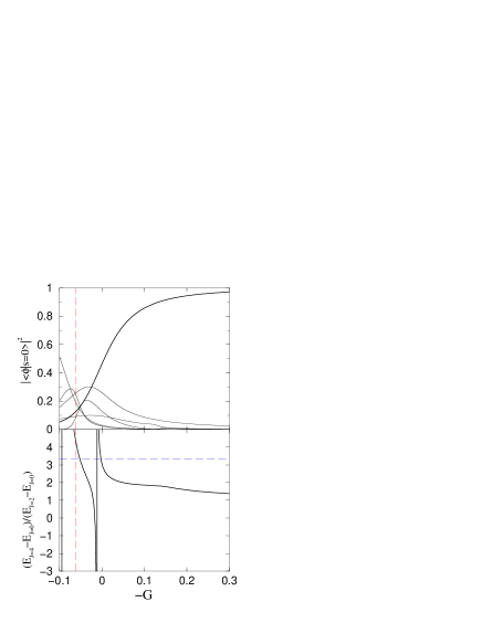
FIG. 5.: Properties of the system of six particles on $j=15/2$ orbital with the P+Q interaction are studied as a function of the parameter $G\,;$ the quadrupole strength is set at $\chi_{2}=1\,.$ The upper plot shows the overlap of all six $J=0$ eigenstates in this system with the $s=0$ pairing state, which is defined as a ground state wave function for the pairing interaction $G=-1\,$ and $\chi_{2}=0\,.$ Lower plot shows the ratio $(E_{J=4}-E_{J=0})/(E_{J=2}-E_{J=0})$ as a function of $G$, here $E_{J=4,2,0}$ are the energies of the lowest states with spin 4, 2, and 0, respectively.

B Pairing and deformation

In this subsection we will investigate the interplay of pairing and deformation in the P+Q model. Rotational bands in the low end of the spectrum, and the Alaga intensity rules will serve us as tools in this study. The lower part of Fig. 5 shows that an indication for a rotational band near the “no pairing” region, $G=0\,.$ Here, judging by the excitation energy, the lowest states with $J=0,2$ and 4 are forming a collective rotational band. As it is clear from the figure this region is very small. Thus, for the most part we will concentrate here on a pure quadrupole-quadrupole interaction

$$H=-\frac{\chi_{2}}{2}\sum_{\kappa}{\cal M}^{\dagger}_{2\,\kappa}{\cal M}_{2\,\kappa}\,,$$ (83)

which, as we have shown above, is still significantly influenced by the kinematic pairing, with the bandhead $J=0$ state dominated by the $s=0$ pairing component.

We note that although single-$j$ model is very limited, an exact rotational spectrum can still be formed using

$$H=\chi_{1}\sum_{\kappa}{\cal M}^{\dagger}_{1\,\kappa}{\cal M}_{1\,\kappa}=\frac{\chi_{1}}{j(j+1)\Omega}J^{2}\,,$$ (84)

which is seniority conserving and, according to Eq. (15) can be defined in the $p-p$ channel with the aid of the set of parameters

$$V_{L}=L(L+1)-2j(j+1)\propto\left\{\begin{array}[]{ccc}j&j&L\\ j&j&1\end{array}\right\}\,.$$ (85)

This interaction remarkably well satisfies the Alaga intensity rules, see below, for reasonably large $j$ and $N\,.$ In the model with random interactions [2, 22], the contributions (85) determine the effective statistical moment of inertia. Similar to this example other odd-multipolarity multipoles can be used to create seniority conserving interactions, this is another way of finding solutions to Eq. (64).

The main hint for the presence of deformation comes from the mean field approximation [21] (with exchange terms ignored by definition of the model this is in fact a Hartree approximation). For axially symmetric deformation, the average values of the multipole moments are

$$\langle{\cal M}_{2\,0}\rangle=\sum_{m}\frac{2(3m^{2}-j(j+1))}{\sqrt{\Omega(\Omega^{2}-1)(\Omega^{2}-2)}}\,n_{m}\,,$$ (86)

in terms of the occupation numbers $n_{m}=\langle a^{\dagger}_{m}\,a_{m}\,\rangle$ in the intrinsic frame with the $z$-axis oriented along the symmetry axis, and

$$\langle{\cal M}_{2\,-2}\rangle=\langle{\cal M}_{2\,2}\rangle=0\,.$$

The single-particle energies in the body-fixed frame can be obtained via the usual self-consistency requirement

$$\epsilon_{m}=-\chi_{2}\,\,\frac{2(3m^{2}-j(j+1))}{\sqrt{\Omega(\Omega^{2}-1)(\Omega^{2}-2)}}\,\langle{\cal M}_{2\,0}\rangle\,.$$ (87)

This problem can be solved exactly [21]. The minimum energy corresponds to the Fermi occupation of the $N$ lowest pairwise degenerate orbitals $|m|=1/2,3/2,\dots(N-1)/2$ for prolate or $|m|=j,j-1,\dots j-(N-2)/2$ for oblate shapes. The corresponding quadrupole moment is then given as

$$\langle{\cal M}_{2\,0}\rangle=-\frac{1}{4}\,\frac{N(\Omega^{2}-N^{2})}{\sqrt{\Omega(\Omega^{2}-1)(\Omega^{2}-4)}}$$ (88)

for prolate deformation and

$$\langle{\cal M}_{2\,0}\rangle=\frac{1}{4}\,\frac{N(2\Omega-N)(\Omega-N)}{\sqrt{\Omega(\Omega^{2}-1)(\Omega^{2}-4)}}$$ (89)

for oblate deformation. The deformation energy, defined as

$$E_{\rm deformation}=-\frac{\chi_{2}}{2}\,|\langle{\cal M}_{2\,0}\rangle|^{2}\,,$$ (90)

shows that oblate deformation is preferred for $N<\Omega/2$ and prolate correspondingly for $N>\Omega/2\,.$ In the middle of the shell there is a phase transition from prolate to oblate deformation. In this region energies associated with prolate and oblate deformation become equal. The average quadrupole moments at this point do not vanish; they are opposite in sign for prolate and oblate deformation. Because of this phase transition, mesoscopic nature of the system, and all other kinematic terms ignored in the model, the true ground state is a superposition of oblate and prolate forms in the region of a half-occupied shell. At the exact point of half-occupancy the particle-hole symmetry requires $\langle{\cal M}_{2\,0}\rangle=0\,$ for the true ground state of the system. The oblate to prolate transition turns out to be advantageous to pairing, as can be seen from Fig. 4. The content of pairing, the $s=0$ component in the wave function, is slightly enhanced in the middle of the shell. This enhancement, being accompanied by strong effects of kinematic pairing near both limits $N=0$ and $N=\Omega\,,$ is largely responsible for the presence of pairing correlations throughout the entire region within a single shell.

The moment of inertia in the cranking approximation, that will be of use in our further discussion, is given by the following expression

$${\cal I}=-\sum_{m\,m^{\prime}}\frac{n_{m}-n_{m^{\prime}}}{\epsilon_{m}-\epsilon_{m^{\prime}}}\,|j_{x}|^{2}\,.$$ (91)

With a sharp Fermi surface only four terms in the sum, $|m|=|m^{\prime}|\pm 1$ will work. Utilizing Eqs. (87) and (9) we obtain

$${\cal I}_{\rm prolate}=\frac{\Omega(\Omega^{2}-1)(\Omega^{2}-4)}{6\,\chi_{2}\,N^{2}}\,,\quad{\cal I}_{\rm oblate}=\,\frac{\Omega(\Omega^{2}-1)(\Omega^{2}-4)}{6\,\chi_{2}\,(\Omega-N)^{2}}\,.$$ (92)

The Elliot’s SU(3) model has a clear rotational structure and can serve as a link for understanding a macroscopic deformation and its microscopic description. In the quadrupole-quadrupole Hamiltonian under consideration the SU(3) algebra is broken in such a kinematic way that boosts competing pairing. The commutator of the quadrupole operators, according to Eq. (12), consists of vector and octupole components

$$[{\cal M}_{2\,\kappa},\,{\cal M}_{2\,\kappa^{\prime}}]=6\,\sum_{q}\,(-)^{q}\,\left\{\begin{array}[]{ccc}2&2&1\\ j&j&j\end{array}\right\}\,\left(\begin{array}[]{ccc}2&2&1\\ \kappa&\kappa^{\prime}&-q\end{array}\right)\,{\cal M}_{1\,q}$$ (93)

$$+14\,\sum_{q}\,(-)^{q}\,\left\{\begin{array}[]{ccc}2&2&3\\ j&j&j\end{array}\right\}\,\left(\begin{array}[]{ccc}2&2&3\\ \kappa&\kappa^{\prime}&-q\end{array}\right)\,{\cal M}_{3\,q}\,.$$

The octupole component is what breaks the SU(3) algebra; ignoring this term, and similar to Eq. (9), introducing a quadrupole operator according to

$${\cal M}_{2\,q}=\frac{{Q}_{q}}{\sqrt{5\,j(j+1)\,\Omega}}\,,$$ (94)

we obtain a SU(3) algebra in the standard form

$$[J_{q}\,,J_{q^{\prime}}]=-\sqrt{2}\,C_{1q,\,1q^{\prime}}^{1q+q^{\prime}}\,J_{q+q^{\prime}}\,$$ (95)

$$[{Q}_{q}\,,J_{q^{\prime}}]=-\sqrt{6}\,C_{2q,\,1q^{\prime}}^{2q+q^{\prime}}\,{Q}_{q+q^{\prime}}\,$$ (96)

$$[{Q}_{q}\,,{Q}_{q^{\prime}}]=3\sqrt{10}\,C_{2q,\,2q^{\prime}}^{1q+q^{\prime}}\,J_{q+q^{\prime}}\,.$$ (97)

The quadrupole-quadrupole Hamiltonian can be expressed via the bilinear Casimir operator of this group

$${\cal C}=Q\cdot Q+3\,J\cdot J\,.$$ (98)

The expectation value of this invariant operator depends only on quantum numbers $\lambda$ and $\mu$ that label representations, see for example [23],

$$\langle{\cal C}\rangle=4(\lambda^{2}+\mu^{2}+\lambda\,\mu+3\lambda+3\mu)\,.$$ (99)

For a given representation $(\lambda\,\mu)\,,$ where $\lambda\geq\mu\,,$ the angular momentum can be

$$L=\left\{\begin{array}[]{lc}K,K+1,K+2,\dots K+\lambda&K\neq 0\,,\cr\lambda,\lambda-2\dots(1\,\,{\rm or}\,\,0)&K=0\,,\cr\end{array}\right.\,$$ (100)

where an integer $K$ takes values $K=\mu,\mu-2,\dots(1\,\,{\rm or}\,\,0)\,.$ Assuming a deformed band based on the ground state $K=0$ we choose $\mu=0$ and $\lambda=N(\Omega-N)/2\,$ where $\lambda$ coincides with the maximum possible value of angular momentum in the system. Thus in the approximation of SU(3) symmetry the expectation value of the quadrupole-quadrupole Hamiltonian becomes

$$\langle N\,(J)|H|N\,(J)\rangle=-\frac{2\,\chi_{2}\,N(\Omega-N)(N\Omega-N^{2}+6)}{5\,\Omega(\Omega^{2}-1)}+\frac{6\,\chi_{2}\,J(J+1)}{5\,\Omega(\Omega^{2}-1)}$$ (101)

The SU(3) model results in exact rotational bands with the $N$-independent moment of inertia

$${\cal I}=\frac{5\Omega(\Omega^{2}-1)}{12\chi_{2}}\,.$$ (102)

In Fig. 6 the moments of inertia obtained from Eqs. (92) and (102) and from fitting the $J=0,2,4$ states in the spectra obtained from exact diagonalization are compared. In a view of the previous discussion it is not surprising that observed moments of inertia are significantly lower than ones predicted by both of the considered models. This effect should be attributed to pairing, which is mainly of a kinematic origin.

FIG. 6.: Moments of inertia obtained using different models and from fitting the low-lying states in the exact spectrum are compared as a function of a number of particles. The pure quadrupole-quadrupole interaction is used ($\chi_{2}=1$ and $G=0$) for the system on a single $j=15/2$ level. The solid line corresponds to the moment of inertia coming from fitting the exact spectrum, short-dashed line corresponds to the moment of inertia from the mean field treatment, and long dashed line is for the SU(3) model, the latter predicts an $N$-independent value.

Static deformation of a nucleus manifests itself via relations (the so-called Alaga intensity rules) between the diagonal expectation values of multipole moments and off-diagonal, transitional amplitudes corresponding to the same $K$ band. We consider here a quadrupole moment of the lowest excited $J=2$ state and the E2 transition between this state and the $J=0$ ground state. In a single level model the quadrupole operator must be proportional to ${\cal M}_{2\,\kappa}$ as it is the only particle-hole operator with the correct rotational properties. We define quadrupole moment of the state as

$${\cal Q}=\langle JM=J|{\cal M}_{2\,0}|J\,M=J\rangle\,.$$ (103)

The B(E2) transition strength is defined as

$${\rm B(E2)}=\sum_{M_{f}\,\kappa}\,|\langle JM_{f}|{\cal M}_{2\,\kappa}|J\,M_{i}|^{2}\,.$$ (104)

The Alaga intensity rules are then expressed via relation [24, 25]

$$\frac{{\cal Q}^{2}}{\rm B(E2)}=\frac{4}{49}\,.$$ (105)

Within the pairing based treatment of interactions which implies no seniority mixing, this ratio can be calculated analytically. We assume that the lowest $J=2$ state has pure seniority $s=2\,.$ Due to the seniority conservation, this is the only state that can directly decay into the ground state, assumed here to have $s=0\,,$ via an E2 transition. The amplitude of this transition is given by

$$\langle s=2,K\kappa|{\cal M}^{\dagger}_{K\,\kappa}|s=0\rangle=-\sqrt{\frac{2N(\Omega-N)}{(2K+1)\Omega(\Omega-2)}}\,,$$ (106)

therefore in the limit of strong pairing

$${\rm B(E2)}=\frac{2N(\Omega-N)}{\Omega(\Omega-2)}\,.$$ (107)

The rate of this transition is maximized for a half-occupied system. The corresponding quadrupole moment in the $J=2$ and $s=2$ state can be determined from

$$\langle N,s=2,(JM)|{\cal M}_{K\,0}|N,s=2,(JM)\rangle$$ (108)

$$=2(2J+1)\,\frac{2N-\Omega}{\Omega-4}\,(-)^{M}\left(\begin{array}[]{ccc}J&K&J\\ M&0&-M\end{array}\right)\left\{\begin{array}[]{ccc}J&K&J\\ j&j&j\end{array}\right\}\,.$$

Application for quadrupole $K=2$ results in the following expression

$${\cal Q}=\frac{4}{7}\,\frac{(2N-\Omega)(\Omega+4)}{\sqrt{\Omega(\Omega^{2}-1)(\Omega^{2}-4)}}\,.$$ (109)

The quadrupole moment goes to zero for the half-occupied shell as required by the particle-hole symmetry.

In general, the paired state is not deformed and thus the B(E2) transition probability in (107) and the quadrupole moment (109) do not satisfy the intensity rule (105). With the quadrupole-quadrupole interaction presented, a deformation can appear and Alaga intensity rules can be fulfilled. In Fig. 7 for the system $j=15/2$ and $N=6\,,$ the quadrupole moment, B(E2) transition strength, and the ratio ${\cal Q}^{2}/{\rm B(E2)}$ are presented as a function of the pairing strength $G\,.$ Dashed lines show the results for the strong pairing limit, obtained using Eqs. (107) and (109).

FIG. 7.: The quadrupole characteristics of the first excited $2^{+}$ state, the diagonal quadrupole moment $Q$, Eq. (97), middle panel, and the reduced transition probability to the ground state, B(E2), Eq. (98), upper panel, in the P+Q model for the single $j=15/2$ level and $N=6\,,$ as a function of pairing strength $G\,.$ Long dashed line on all plots indicates the results from pairing based description. The lower plot shows the prediction of the Alaga intensity rule $Q^{2}/{\rm B(E2)}=4/49\,,$ short dashed line.

Fig. 8 compares the behavior of the ratio $Q^{2}/{\rm B(E2)}$ as a function of the pairing strength $G$ in different systems $N=2,4,6,8,10$ with $j=21/2\,.$ There are two special cases. For $N=2$ (the same is true for $N=\Omega-2\,$) the ground state is paired, and the Alaga ratio is determined exactly via Eqs. (107) and (109). The second case is for $N=\Omega/2\,,$ where due to particle-hole symmetry $Q^{2}/{\rm B(E2)}=0\,.$ For all other situations Alaga intensity rules are fulfilled to a sufficient degree of accuracy for the pure quadrupole-quadrupole Hamiltonian $G=0\,.$ As the pairing strength increases, the ratio $Q^{2}/{\rm B(E2)}$ moves away from the Alaga value towards the limit determined by pairing, which is shown by thin dashed lines. Curves corresponding to systems with a number of particles close to $N=2\,$ ($N=\Omega-2\,$) or $N=\Omega/2\,$ converge to the pairing limit significantly faster. This fact is yet another manifestation of preference for pairing correlations in these systems.

FIG. 8.: Ratio $Q^{2}/{\rm B(E2)}$ for systems with different numbers of particles $N$ on a single $j=21/2$ level is plotted in solid lines as a function of pairing strength $G\,.$ Thin dashed lines, with corresponding values of $N$ marked on the right, indicate the intensity ratios for corresponding systems in the limit of validity of pairing perturbation theory. All results should be compared with $Q^{2}/B(E2)=4/49\approx 0.082\,,$ the Alaga intensity ratio of a rotating rigid body.

V Conclusions

The pairing interaction is a very important part of the general residual interaction. However the fact that many nuclei are paired in their ground or low-lying exited states is a result of a non-trivial interplay of pairing matrix elements and other parts of the residual interaction, as well as kinematic constraints. It has been earlier shown through a number of numerical studies that the realistic interaction is different from an arbitrary symmetry preserving random interaction. The difference lies in the correlations between the interaction parameters that exist even in the truncated shell model space, reflecting the overall properties of the nuclear medium. Interactions that permit paired states and allow for deformations produce very correlated sets of residual two-body matrix elements. Apart from the dynamic correlations there are kinematic couplings between different collective modes, that mainly appear from the geometrical restrictions imposed on collective excitations.

In many realistic systems pairing is relatively weak compared to the critical value of phase transition defined by BCS. However, as was shown by numerous authors, pairing correlations in mesoscopic systems extend far beyond the BCS phase transition. This makes the exact treatment of pairing a necessary component in the study of a sensitive interplay between pairing and other interactions.

The simple single-level systems considered in this work has served as an excellent testing ground. The SU(2) quasispin algebra allows for an exact solution of the pairing problem, and perturbation theory based on the paired state [5] can be further developed with ease. This makes it possible to address important questions of the stability of the paired state as well as to investigate dynamic renormalizations of two-body interactions in the presence of the pairing condensate.

The interaction parameters for a one-level system in the particle-particle and particle-hole channels can be related to each other, revealing kinematic constraints in a simple form. Additional restrictions on the behavior of the system come from the exact particle-hole symmetry. As a result of this symmetry, all multipole moments of even multipolarity are identically zero for a half-occupied shell. These constraints turned out to be very important for the preservation of pairing in the presence of deformation. Interplay of pairing and deformation was discussed using the P+Q model. The particular case of this model, the pure quadrupole-quadrupole interaction with no explicit pairing, has been addressed in detail. This interaction was expected to be the one most “orthogonal” to pairing; however, strong evidence of pairing correlations was found even in this case. We have shown that the pairing is the strongest attractive component in the quadrupole-quadrupole interaction when the latter is converted from the $p-h$ to $p-p$ channel. This means that for any attractive, i.e. favoring deformation, quadrupole-quadrupole interaction on a single $j$-level, the ground state of a two particle or two-hole system is a paired state ($J=0$ and $s=0\,$). The same is in fact true for a more general Hamiltonian containing any attractive multipole-multipole interaction of even multipolarity. This results in enhanced pairing correlations in near-magic configurations. An additional enhancement of pairing was observed in the systems close to the half-filled shell. This is related to the prolate-oblate phase transition taking place in this region; it weakens deformation thus allowing for more pairing. A number of calculations was performed to emphasize the discussed aspects, and the results were compared to the predictions of the mean field approximation and Elliot’s SU(3) model. Direct overlaps with the $s=0$ paired wave-function, excitation spectrum, intensities of transitions and moments of inertia all indicate an appearance of pairing, consistent with the kinematic constraints.

The simple model used in this work is only a very limited approximation to the situation in nuclear systems. However, the observed effects of pairing enhancement via kinematic or dynamic interplay with other interactions have to exist to some extent in realistic systems. The situation in the realistic shell model becomes much more diverse as it is complicated by an increasingly large number of interaction parameters, weakening of antisymmetry requirements and other kinematic restrictions, and a diversity of collective modes. Pairing itself becomes different, isovector and isoscalar pairing modes can compete, the pairing state of the lowest total seniority $s=0$ is not unique and can involve coherent and incoherent pair vibrations [26] which, under effects of other interactions, may result in a paired condensate that is different from the prediction of the regular BCS.

Acknowledgements: The author wishes to thank V. Zelevinsky, B. A. Brown and D. Mulhall for motivating discussions and useful criticism, without their help this work would not be possible. The NSF support of this research is greatly appreciated.

REFERENCES

- [1] S. T. Belyaev, Yad. Phys. 4, 936 (1966), [Sov. J. Nucl. Phys. 4, 671 (1967)]; S. T. Belyaev, Phys. Lett. B 28, 365 (1969).
- [2] D. Mulhall, A. Volya and V. Zelevinsky, Phys. Rev. Lett. 85, 4016 (2000).
- [3] M. Horoi, B. A. Brown, and V. Zelevinsky, Phys. Rev. Lett. 87, 062501 (2001).
- [4] S. G. Kadmenskii, P. A. Luk’yanovich, Yu. I. Remesov, and V. I. Furman, Sov. J. Nucl. Phys. 45, 585 (1987).
- [5] A. Volya, B. A. Brown, and V. Zelevinsky, Phys. Lett. B 509, 37 (2001).
- [6] S. G. Kadmenskii and P. A. Luk’yanovich, Sov. J. Nucl. Phys. 49 (2), 238 (1989).
- [7] F. Barranco, R. A. Broglia, G. Gori, E. Vigezzi, P. F. Bortignon, and J. Terasaki, Phys. Rev. Lett. 83, 2147 (1999).
- [8] S. P. Pandya, Phys. Rev. 103, 956 (1956).
- [9] S. T. Belyaev, J. Exptl. Theoret. Phys. (USSR) 39, 1387; JETP 12, 963 (1962).
- [10] A. de-Shalit and I. Talmi, Nuclear Shell Theory (Academic Press, New York, 1963).
- [11] G. F. Bertsch, The Practitioner’s Shell Model (North-Holland, Amsterdam, 1972).
- [12] R. D. Lawson, Theory of the Nuclear Shell Mondel (Clarendon Press, Oxford, 1980).
- [13] J. Bardeen, L.N. Cooper and J.R. Schrieffer, Phys. Rev. 108, 1175 (1957).
- [14] G. Racah, Phys. Rev. 62, 438 (1942); Phys. Rev. 63, 367 (1943).
- [15] A. K. Kerman, R. D. Lawson, and M. H. Macfarlane, Phys. Rev. 124, 162 (1961).
- [16] I. Talmi, Simple Models of Complex Nuclei (Hartwood Academic Publishers, Chur, 1993).
- [17] D. J. Rowe and G. Rosensteel, Phys. Rev. Lett. 87, 172501 (2001).
- [18] C. W. Johnson, G. F. Bertsch, D. J. Dean, and I. Talmi, Phys. Rev. C 61, 014311 (2000).
- [19] I. Talmi, Nucl. Phys. A686, 217 (2001).
- [20] P. Ring and P. Schuck, The Nuclear Many-Body Problem, (Springer-Verlag, New York, 1980).
- [21] M. Baranger, K. Kumar, Nucl. Phys. 62, 113 (1965).
- [22] V. Zelevinsky, D. Mulhall, and A. Volya, Yad. Phys. 63, 579 (2001) [Physics of Atomic Nuclei 64, 525 (2001)].
- [23] J. P. Elliot, Selected Topics in Nuclear Theory (International Atomic Energy Agency, Vienna, 1963).
- [24] V. Zelevinsky, Introduction to Nuclear Theory, lecture course (Niels Bohr Institite, University of Copenhagen, 1995).
- [25] A. Bohr and B. Mottelson, Nuclear Structure, Vol. 2 (Benjamin, New York, 1974).
- [26] A. Volya, V. Zelevinsky, B. A. Brown, LANL preprint nucl-th/0109022.