HFB Calculations Near the Drip Lines

Abstract

We present the first set of results of solving the Hartree-Fock-Bogoliubov equations, which describe the self-consistent mean field theory with pairing interaction. Calculations for even-even nuclei are carried out on a two-dimensional axially symmetric lattice, in coordinate space. An important aspect of our method is the proper representation of the quasi-particle continuum wavefunctions, which are considered for energies up to 60 MeV. This stage is essential for a proper description of nuclei near the drip lines, due to the strong coupling between weakly bound states and the particle continuum for such nuclei. High accuracy is achieved by representing the operators and wavefunctions using the technique of basis-splines. Calculations for $Sn$ isotopes are presented to demonstrate the reliability of the method.

1 Introduction

The study of structures and reactions of nuclei far from stability has been one of the most active fields of nuclear physics in the past decade [1, 2]. The microscopic description of such nuclei will lead to a better understanding of the interplay among the strong, Coulomb, and the weak interactions as well as the enhanced correlations present in these many-body systems.

The experimental developments as well as recent advances in computational physics have sparked renewed interest in nuclear structure theory. In contrast to the well-understood behavior near the valley of stability, there are many open questions as we move towards the proton and neutron driplines and towards the limits in mass number. The neutron dripline represents mostly “terra incognita”. In these exotic regions of the nuclear chart, some of the topics of interest are the effective N-N interaction at large isospin, large pairing correlations and their density dependence, neutron halos/skins, and proton radioactivity. Specifically, we are interested in calculating ground state observables such as the total binding energy, charge radii, proton and neutron densities, separation energies for neutrons and protons, pairing gaps, and potential energy surfaces. It is generally acknowledged that an accurate treatment of the pairing interaction is essential for describing exotic nuclei [3, 4].

In Section 2 the general outline of the HFB formalism is shown in second quantization and its representation in coordinate space. Section 3 shows the reduction of the HFB equations for cylindrical coordinates. The last two sections include results and discussion of our HFB calculations.

2 Hartree-Fock-Bogoliubov Formalism

2.1 Basic outline of HFB equations

The many-body Hamiltonian in occupation number representation has the form

$$\hat{H}=\sum_{i,j}<i|\ t\ |j>\ \hat{c}_{i}^{\dagger}\ \hat{c}_{j}\ +\frac{1}{4}\sum_{i,j,m,n}<ij|\ \tilde{v}^{(2)}\ |mn>\ \hat{c}_{i}^{\dagger}\ \hat{c}_{j}^{\dagger}\ \hat{c}_{n}\ \hat{c}_{m}\ +\ ...$$ (1)

Similar to the BCS theory, one performs a canonical transformation to quasiparticle operators $\hat{\beta},\hat{\beta}^{\dagger}$

$$\left(\begin{array}[]{c}\hat{\beta}\\ \hat{\beta}^{\dagger}\end{array}\right)=\left(\begin{array}[]{cc}U^{\dagger}&V^{\dagger}\\ V^{T}&U^{T}\end{array}\right)\left(\begin{array}[]{c}\hat{c}\\ \hat{c}^{\dagger}\end{array}\right)\ .$$ (2)

The HFB ground state is defined as the quasiparticle vacuum

$$\hat{\beta}_{k}\ |\Phi_{0}>\ =\ 0\ .$$ (3)

The HFB ground state energy together with the constraint on the particle number is given by

$$E({\mathcal{R}})=<\Phi_{0}|\hat{H}-\lambda\hat{N}|\Phi_{0}>\ ,$$ (4)

where $\mathcal{R}$ is the generalized density matrix, function of the normal density $\rho_{i,j}$ and the pairing tensor $\kappa_{i,j}$. We derive the equations of motion from the variational principle

$$\delta\ [E({\mathcal{R}})-{\rm{tr}}\ \Lambda({\mathcal{R}}^{2}-{\mathcal{R}})]=0\ ,$$ (5)

which results in the standard HFB equations

$$[{\mathcal{H}},{\mathcal{R}}]\ =\ 0\ ,$$ (6)

with the generalized single-particle Hamiltonian

$${\mathcal{H}}=\left(\begin{array}[]{cc}(h-\lambda)&\tilde{h}\\ \tilde{h}&-(h-\lambda)\ ,\end{array}\right)\ ,$$ (7)

where $h$ and $\tilde{h}$ denote the particle and pairing Hamiltonians, respectively and the Lagrange multiplier $\lambda$ is the Fermi energy.

2.2 HFB equations in coordinate space

For certain types of effective interactions (e.g. Skyrme mean field and pairing delta-interactions) the “particle” Hamiltonian $h$ and the “pairing” Hamiltonian $\tilde{h}$ are diagonal in isospin space and local in position space,

$$h({\bf r}\sigma q,{\bf r}^{\prime}\sigma^{\prime}q^{\prime})\ =\ \delta_{q,q^{\prime}}\ \delta({\bf r}-{\bf r}^{\prime})h^{q}_{\sigma,\sigma^{\prime}}({\bf r})$$ (8)

and

$$\tilde{h}({\bf r}\sigma q,{\bf r}^{\prime}\sigma^{\prime}q^{\prime})\ =\ \delta_{q,q^{\prime}}\ \delta({\bf r}-{\bf r}^{\prime})\tilde{h}^{q}_{\sigma,\sigma^{\prime}}({\bf r})\ .$$ (9)

Inserting these into the above HFB equations results in a 4x4 structure in spin space:

$$\left(\matrix{(h^{q}-\lambda)&\tilde{h}^{q}\cr\tilde{h}^{q}&-(h^{q}-\lambda)\cr}\right)\left(\matrix{\phi^{q}_{1,\alpha}\cr\phi^{q}_{2,\alpha}\cr}\right)=E_{\alpha}\left(\matrix{\phi^{q}_{1,\alpha}\cr\phi^{q}_{2,\alpha}\cr}\right)\ ,$$ (10)

with

$$h^{q}=\left(\matrix{h^{q}_{\uparrow\uparrow}({\bf r})&h^{q}_{\uparrow\downarrow}({\bf r})\cr h^{q}_{\downarrow\uparrow}({\bf r})&h^{q}_{\downarrow\downarrow}({\bf r})\cr}\right)\ ,\ \ \ \tilde{h}^{q}=\left(\matrix{\tilde{h}^{q}_{\uparrow\uparrow}({\bf r})&\tilde{h}^{q}_{\uparrow\downarrow}({\bf r})\cr\tilde{h}^{q}_{\downarrow\uparrow}({\bf r})&\tilde{h}^{q}_{\downarrow\downarrow}({\bf r})\cr}\right)$$ (11)

and

$$\phi^{q}_{1,\alpha}=\left(\matrix{\phi^{q}_{1,\alpha}({\bf r},\uparrow)\cr\phi^{q}_{1,\alpha}({\bf r},\downarrow)\cr}\right)\ ,\ \ \ \phi^{q}_{2,\alpha}=\left(\matrix{\phi^{q}_{2,\alpha}({\bf r},\uparrow)\cr\phi^{q}_{2,\alpha}({\bf r},\downarrow)\cr}\right)\ .$$ (12)

Because of the structural similarity between the Dirac equation and the HFB equation in coordinate space, we encounter here similar computational challenges: for example, the spectrum of quasiparticle energies $E$ is unbounded from above and below. The spectrum is discrete for $|E|<-\lambda$ and continuous for $|E|>-\lambda$. For even-even nuclei it is customary to solve the HFB equations with a positive quasiparticle energy spectrum $+E_{\alpha}$ [5] and consider all negative energy states as occupied in the HFB ground state.

3 2-D Reduction for Axially Symmetric Systems

For simplicity, we assume that the HFB quasi-particle Hamiltonian is invariant under rotations ${\hat{R}}_{z}$ around the z-axis, i.e. $[{\mathcal{H}},{\hat{R}}_{z}]=0$. Due to the axial symmetry of the problem, it is advantageous to introduce cylindrical coordinates $(\phi,r,z)$.

It is possible to construct simultaneous eigenfunctions of the generalized Hamiltonian ${\mathcal{H}}$ and the z-component of the angular momentum, ${\hat{j}}_{z}$

$${\mathcal{H}}\ \psi_{n,\Omega,q}(\phi,r,z) = E_{n,\Omega,q}\ \psi_{n,\Omega,q}(\phi,r,z)$$

$${\hat{j}}_{z}\ \psi_{n,\Omega,q}(\phi,r,z) = \hbar\Omega\ \psi_{n,\Omega,q}(\phi,r,z)\ ,$$ (13)

with the quantum numbers $\Omega=\pm\frac{1}{2},\pm\frac{3}{2},\pm\frac{5}{2},...$. The simultaneous quasiparticle eigenfunctions take the form

$$\psi_{n,\Omega,q}(\phi,r,z)=\left(\begin{array}[]{c}\phi^{(1)}_{n,\Omega,q}(\phi,r,z)\\ \phi^{(2)}_{n,\Omega,q}(\phi,r,z)\\ \end{array}\right)=\frac{1}{\sqrt{2\pi}}\left(\begin{array}[]{c}e^{i(\Omega-\frac{1}{2})\phi}\ \phi^{(1)}_{n,\Omega,q}(r,z,\uparrow)\\ e^{i(\Omega+\frac{1}{2})\phi}\ \phi^{(1)}_{n,\Omega,q}(r,z,\downarrow)\\ e^{i(\Omega-\frac{1}{2})\phi}\ \phi^{(2)}_{n,\Omega,q}(r,z,\uparrow)\\ e^{i(\Omega+\frac{1}{2})\phi}\ \phi^{(2)}_{n,\Omega,q}(r,z,\downarrow)\end{array}\right)\ .$$ (14)

We introduce the following useful notation

$$U^{(1,2)}_{n\Omega q}(r,z)=\phi^{(1,2)}_{n,\Omega,q}(r,z,\uparrow)\ ,\ L^{(1,2)}_{n\Omega q}(r,z)=\phi^{(1,2)}_{n,\Omega,q}(r,z,\downarrow)\ .$$ (15)

From the vanishing commutator, $[{\mathcal{H}},j_{z}]$, we can determine the $\phi$-dependence of the HFB quasi-particle Hamiltonian and arrive at the following structure for the Hamiltonian

$$h(\phi,r,z)=\left(\begin{array}[]{cc}h^{\prime}_{\uparrow\uparrow}\ (r,z)&e^{-i\phi}\ h^{\prime}_{\uparrow\downarrow}\ (r,z)\\ e^{+i\phi}\ h^{\prime}_{\downarrow\uparrow}\ (r,z)&h^{\prime}_{\downarrow\downarrow}\ (r,z)\end{array}\right)\ .$$ (16)

and the pairing Hamiltonian

$$\tilde{h}(\phi,r,z)=\left(\begin{array}[]{cc}\tilde{h}^{\prime}_{\uparrow\uparrow}\ (r,z)&e^{-i\phi}\ \tilde{h}^{\prime}_{\uparrow\downarrow}\ (r,z)\\ e^{+i\phi}\ \tilde{h}^{\prime}_{\downarrow\uparrow}\ (r,z)&\tilde{h}^{\prime}_{\downarrow\downarrow}\ (r,z)\end{array}\right)\ ,$$ (17)

Inserting equations (16) and (17) into the eigenvalue Eq. (10) , we arrive at the “reduced 2-D problem” [9] in cylindrical coordinates:

$$\left(\matrix{(h^{\prime}_{\uparrow\uparrow}-\lambda)&h^{\prime}_{\uparrow\downarrow}&\tilde{h^{\prime}}_{\uparrow\uparrow}&\tilde{h^{\prime}}_{\uparrow\downarrow}\cr h^{\prime}_{\downarrow\uparrow}&(h^{\prime}_{\downarrow\downarrow}-\lambda)&\tilde{h^{\prime}}_{\downarrow\uparrow}&\tilde{h^{\prime}}_{\downarrow\downarrow}\cr\tilde{h^{\prime}}_{\uparrow\uparrow}&\tilde{h^{\prime}}_{\uparrow\downarrow}&-(h^{\prime}_{\uparrow\uparrow}-\lambda)&-h^{\prime}_{\uparrow\downarrow}\cr\tilde{h^{\prime}}_{\downarrow\uparrow}&\tilde{h^{\prime}}_{\downarrow\downarrow}&-h^{\prime}_{\downarrow\uparrow}&-(h^{\prime}_{\downarrow\downarrow}-\lambda)\cr}\right)\left(\matrix{U^{(1)}_{n,\Omega,q}\cr L^{(1)}_{n,\Omega,q}\cr U^{(2)}_{n,\Omega,q}\cr L^{(2)}_{n,\Omega,q}\cr}\right)=E_{n,\Omega,q}\ \left(\matrix{U^{(1)}_{n,\Omega,q}\cr L^{(1)}_{n,\Omega,q}\cr U^{(2)}_{n,\Omega,q}\cr L^{(2)}_{n,\Omega,q}\cr}\right)$$

Here $\tilde{h^{\prime}}$, $h^{\prime}$, $U$’s, and $L$’s are all functions of $(r,z)$ only. For a given angular momentum projection quantum number $\Omega$, we solve the eigenvalue problem to obtain energy eigenvalues $E_{n,\Omega,q}$ and eigenvectors $\psi_{n,\Omega,q}$ for the HFB quasi-particle states.

3.1 HFB Hamiltonian using the Skyrme interaction

Using the Skyrme form for the particle Hamiltonian, $h_{q}$, we can write

$$h_{q}=-{\bf\nabla\cdot}\frac{\hbar^{2}}{2m_{q}^{*}}{\bf\nabla}+U_{q}+U_{C}-i{\bf B}_{q}{\bf\cdot}\left({\bf\nabla\times\sigma}\right)\;\;.$$ (18)

where the effective mass is defined by

$$\frac{\hbar^{2}}{2m_{q}^{*}}=\frac{\hbar^{2}}{2m_{q}}+\frac{1}{4}(t_{1}+t_{2})\rho+\frac{1}{8}(t_{2}-t_{1})\rho_{q}\;\;.$$ (19)

Applying the cylindrical form of the Laplacian operator to the standard form of the wavefunction in Eq.(14), and invoking the axial symmetry of $f$ we find

$$\hat{t}_{q}=\left(\begin{array}[]{cc}t_{11}&0\\ 0&t_{22}\end{array}\right)$$ (20)

where the elements are given by

$$t_{11} = f\left(\frac{\partial^{2}}{\partial r^{2}}+\frac{1}{r}\frac{\partial}{\partial r}-\left(\frac{(\Omega-1/2)}{r}\right)^{2}+\frac{\partial^{2}}{\partial z^{2}}\right)+\frac{\partial f}{\partial r}\frac{\partial}{\partial r}+\frac{\partial f}{\partial z}\frac{\partial}{\partial z}$$ (21)

$$t_{22} = f\left(\frac{\partial^{2}}{\partial r^{2}}+\frac{1}{r}\frac{\partial}{\partial r}-\left(\frac{(\Omega+1/2)}{r}\right)^{2}+\frac{\partial^{2}}{\partial z^{2}}\right)+\frac{\partial f}{\partial r}\frac{\partial}{\partial r}+\frac{\partial f}{\partial z}\frac{\partial}{\partial z}\ ,$$ (22)

$f$ being the effective mass. The local potential terms could also be cast into a matrix form

$$\hat{v}_{q}=\left(\begin{array}[]{cc}v_{11}&0\\ 0&v_{22}\end{array}\right)\ ,$$ (23)

where

$$v_{11}=v_{22}=U_{q}+U_{C}\;\;.$$ (24)

The individual terms are constructed simply by summing appropriately weighted scalars as indicated by Eqs. (3.1) and including the Coulomb potential and the Slater exchange (26) term:

$$U_{q} = t_{0}\left[\left(1+\frac{1}{2}x_{0}\right)\rho-\left(\frac{1}{2}+x_{0}\right)\rho_{q}\right]$$

$$+ \frac{1}{4}\left(t_{1}+t_{2}\right)\tau-\frac{1}{8}\left(t_{1}-t_{2}\right)\tau_{q}$$

$$+ \frac{1}{12}t_{3}\left(1+\frac{1}{2}x_{3}\right)\left(\alpha+2\right)\rho^{\alpha+1}$$

$$- \frac{1}{12}t_{3}\left(\frac{1}{2}+x_{3}\right)\left[\alpha\rho^{\alpha-1}\sum_{q}\rho_{q}^{2}+2\rho^{\alpha}\rho_{q}\right]$$

$$- \frac{1}{2}t_{4}\left[{\bf\nabla\cdot J+\nabla\cdot J}_{q}\right]$$

$$+ \frac{1}{8}\left(t_{2}-3t_{1}\right)\nabla^{2}\rho+\frac{1}{16}\left(t_{2}+3t_{1}\right)\nabla^{2}\rho_{q}\;\;,$$

$$U_{C}=e^{2}\int d^{3}r^{\prime}\frac{\rho_{p}({\bf r^{\prime}})}{|{\bf r}-{\bf r^{\prime}}|}-e^{2}\left(\frac{3}{\pi}\right)^{1/3}\left[\rho_{p}({\bf r})\right]^{1/3}\;\;.$$ (26)

The Hartree-Fock spin-orbit operator

$$-i{\bf B}_{q}{\bf\cdot}\left({\bf\nabla\times\sigma}\right)\longrightarrow\hat{w}_{q}\;\;,$$ (27)

could similarly be cast into the form

$$\hat{w}_{q}=\left(\begin{array}[]{cc}w_{11}&w_{12}\\ w_{21}&w_{22}\end{array}\right)\ ,$$ (28)

with

$$w_{11} = {\cal B}_{r}\frac{\Omega-1/2}{r}$$

$$w_{12} = \left[-{\cal B}_{z}\frac{\Omega+1/2}{r}-{\cal B}_{z}\frac{\partial}{\partial r}+{\cal B}_{r}\frac{\partial}{\partial z}\right]$$

$$w_{21} = \left[-{\cal B}_{z}\frac{\Omega-1/2}{r}+{\cal B}_{z}\frac{\partial}{\partial r}-{\cal B}_{r}\frac{\partial}{\partial z}\right]$$

$$w_{22} = -{\cal B}_{r}\frac{\Omega+1/2}{r}\ ,$$

where

$${\cal B}_{r}\equiv{\bf B_{q}\cdot e_{r}}=\nabla_{r}\frac{t_{4}}{2}(\rho+\rho_{q})\ \ \ ,\ \ \ {\cal B}_{z}\equiv{\bf B_{q}\cdot e_{z}}=\nabla_{z}\frac{t_{4}}{2}(\rho+\rho_{q})\ \ .$$ (29)

3.2 Densities and currents

While the form of the single particle Hamiltonian remains the same as Skyrme HF Hamiltonian, the densities and currents need to be written in terms of the quasi-particle wavefunctions. We obtain the following expressions for the normal density $\rho_{q}({\bf r})$ and pairing density $\tilde{\rho}_{q}({\bf r})$, which are defined as the spin-averaged diagonal elements

$$\rho_{q}({\bf r})\ =\ \sum_{\sigma}\rho({\bf r}\sigma q,{\bf r}\sigma q)\ =\ \sum_{\sigma}\sum_{\alpha}\phi_{2,\alpha}({\bf r}\sigma q)\ \phi_{2,\alpha}^{*}({\bf r}\sigma q)$$ (30)

and

$$\tilde{\rho_{q}}({\bf r})\ =\ \sum_{\sigma}\tilde{\rho}({\bf r}\sigma q,{\bf r}\sigma q)\ =\ -\sum_{\sigma}\sum_{\alpha}\phi_{2,\alpha}({\bf r}\sigma q)\ \phi_{1,\alpha}^{*}({\bf r}\sigma q)\ .$$ (31)

The physical interpretation of $\tilde{\rho_{q}}$ has been discussed in [4]: the quantity $[\tilde{\rho_{q}}({\bf r})\ \Delta V/2]^{2}$ gives the probability to find a correlated pair of nucleons with opposite spin projection in the volume element $\Delta V$.

Using the structure of the bi-spinor wavefunctions defined earlier we find the following expressions for the normal and pairing densities.

$$\rho_{q}(r,z)=\frac{1}{2\pi}\left(2\sum_{\Omega>0}^{\Omega_{max}}\right)\sum_{E_{n}>0}^{E_{max}}\left[|U^{(2)}_{n\Omega q}(r,z)|^{2}+|L^{(2)}_{n\Omega q}(r,z)|^{2}\right]\\$$ (32)

$$\tilde{\rho}_{q}(r,z)=-\frac{1}{2\pi}\left(2\sum_{\Omega>0}^{\Omega_{max}}\right)\sum_{E_{n}>0}^{E_{max}}\left[U^{(2)}_{n\Omega q}(r,z)U^{(1)*}_{n\Omega q}(r,z)+L^{(2)}_{n\Omega q}(r,z)L^{(1)*}_{n\Omega q}(r,z)\right]\ .$$ (33)

Similarly, the kinetic energy density and the divergence of the current become

$$\tau_{q}({\bf r})\ =\ \nabla\cdot\nabla^{\prime}\rho_{q}({\bf r},{\bf r}^{\prime})|_{{\bf r}={\bf r}^{\prime}}\ =\ \sum_{\sigma}\sum_{\alpha}|\nabla\ \phi_{2,\alpha}({\bf r}\sigma q)|^{2}\ ,$$ (34)

$$\tau_{q}(r,z)=\frac{1}{2\pi}\left(2\sum_{\Omega>0}^{\Omega_{max}}\right)\sum_{E_{n}>0}^{E_{max}}\left[\frac{(\Omega-1/2)^{2}}{r^{2}}\left|U^{(2)}_{n\Omega q}\right|^{2}+\frac{(\Omega+1/2)^{2}}{r^{2}}\left|L^{(2)}_{n\Omega q}\right|^{2}\right.$$

$$\left.+\left|\frac{\partial U^{(2)}_{n\Omega q}}{\partial r}\right|^{2}+\left|\frac{\partial L^{(2)}_{n\Omega q}}{\partial r}\right|^{2}+\left|\frac{\partial U^{(2)}_{n\Omega q}}{\partial z}\right|^{2}+\left|\frac{\partial L^{(2)}_{n\Omega q}}{\partial z}\right|^{2}\right]$$ (35)

$$\nabla\cdot{\bf J}_{q}({\bf r})=\frac{1}{2\pi}\left(2\sum_{\Omega>0}^{\Omega_{max}}\right)\sum_{E_{n}>0}^{E_{max}}2\left[\frac{\partial U^{(2)}_{n\Omega q}}{\partial r}\frac{\partial L^{(2)}_{n\Omega q}}{\partial z}-\frac{\partial L^{(2)}_{n\Omega q}}{\partial r}\frac{\partial U^{(2)}_{n\Omega q}}{\partial z}\right.$$

$$+\left.\frac{\Omega-1/2}{r}U^{(2)}_{n\Omega q}\left(\frac{\partial U^{(2)}_{n\Omega q}}{\partial r}-\frac{\partial L^{(2)}_{n\Omega q}}{\partial z}\right)-\frac{\Omega+1/2}{r}L^{(2)}_{n\Omega q}\left(\frac{\partial U^{(2)}_{n\Omega q}}{\partial z}+\frac{\partial L^{(2)}_{n\Omega q}}{\partial r}\right)\right].$$

The total number of protons and neutrons is obtained by integrating over their densities

$$N_{q}=\int d^{3}r\ \rho_{q}({\bf r})=2\pi\int_{0}^{\infty}rdr\int_{-\infty}^{\infty}dz\ \rho_{q}(r,z)$$ (36)

Finally, we state the normalization condition for the four-spinor quasiparticle wavefunctions as

$$\int d^{3}r\ \psi^{\dagger}_{n\Omega q}({\bf r})\ \psi_{n\Omega q}({\bf r})\ =\ 1$$ (37)

which leads to

$$\int_{0}^{\infty}rdr\int_{-\infty}^{\infty}dz\left[|U^{(1)}_{n\Omega q}(r,z)|^{2}+|L^{(1)}_{n\Omega q}(r,z)|^{2}+|U^{(2)}_{n\Omega q}(r,z)|^{2}+|L^{(2)}_{n\Omega q}(r,z)|^{2}\right]\ =\ 1\ .$$

3.3 Pairing interaction.

If one assumes that the effective interaction $\bar{v}^{(2)}_{pair}$ is local,

$$\bar{v}^{(2)}_{pair}({\bf r}\sigma,{\bf r}^{\prime}-\sigma^{\prime};{\bf r_{1}}^{\prime}\sigma_{1}^{\prime},{\bf r_{2}}^{\prime}-\sigma_{2}^{\prime})\ =\ \delta({\bf r_{1}}^{\prime}-{\bf r})\ \delta_{\sigma_{1}^{\prime},\sigma}\ \delta({\bf r_{2}}^{\prime}-{\bf r}^{\prime})\ \delta_{\sigma_{2}^{\prime},\sigma^{\prime}}V_{p}({\bf r}\sigma,{\bf r}^{\prime}-\sigma^{\prime})$$

one finds the following expression for the pairing mean field

$$\tilde{h}({\bf r}\sigma,{\bf r}^{\prime}\sigma^{\prime})\ =\ V_{p}({\bf r}\sigma,{\bf r}^{\prime}-\sigma^{\prime})\ \tilde{\rho}({\bf r}\sigma,{\bf r}^{\prime}\sigma^{\prime})\ .$$ (38)

For the local pairing interaction $V_{p}$ we utilize

$$V_{p}({\bf r}\sigma,{\bf r}^{\prime}-\sigma^{\prime})\ =\ V_{0}\ \delta({\bf r}-{\bf r}^{\prime})\ \delta_{\sigma,\sigma^{\prime}}\ F({\bf r})\ .$$ (39)

This parameterization describes two primary pairing forces: a pure delta interaction ($F=1$) that gives rise to volume pairing, and a density dependent delta interaction (DDDI) that gives rise to surface pairing. The DDDI interaction generates the following pairing mean field for the two isospin orientations $q=\pm\frac{1}{2}$

$$\tilde{h}_{q}({\bf r}\sigma,{\bf r}^{\prime}\sigma^{\prime})\ =\ \frac{1}{2}\ V_{0}^{(q)}\tilde{\rho_{q}}({\bf r})F({\bf r})\ \delta({\bf r}-{\bf r}^{\prime})\ \delta_{\sigma,\sigma^{\prime}}\;\;.$$ (40)

The pairing contribution to the nuclear binding energy is

$$E_{pair}=E_{pair}^{(p)}+E_{pair}^{(n)}=\int d^{3}r\left[\frac{V_{0}^{(p)}}{4}\tilde{\rho}_{p}^{\ 2}({\bf r})+\frac{V_{0}^{(n)}}{4}\tilde{\rho}_{n}^{\ 2}({\bf r})\right]F({\bf r})\ .$$ (41)

3.4 Lattice representation of spinor wavefunctions and Hamiltonian

For a given angular momentum projection quantum number $\Omega$, we solve the eigenvalue problem on a 2-D grid $(r_{\alpha},z_{\beta})$ where $\alpha=1,...,N_{r}$ and $\beta=1,...,N_{z}$. The four components of the spinor wavefunction $\psi(r,z)$ are represented on the 2-D lattice by a product of Basis Spline functions $B_{i}(x)$ evaluated at the lattice support points. Further details are given in Ref. [11].

For the lattice representation of the Hamiltonian, we use a hybrid method [10, 11] in which derivative operators are constructed using the Galerkin method; this amounts to a global error reduction. Local potentials are represented by the B-Spline collocation method (local error reduction). The lattice representation transforms the differential operator equation into a matrix form

$$\sum_{\nu=1}^{N}{\cal{H}}_{\mu}^{\ \nu}\psi^{\Omega}_{\nu}=E^{\Omega}_{\mu}\psi^{\Omega}_{\mu}\ \ \ (\mu=1,...,N)\ ,$$ (42)

with $N=4\times N_{r}\times N_{z}$. The method of direct diagonalization with LAPACK is implemented to solve this eigenvalue problem. Our HFB code is written in Fortran 90 and makes extensive use of new data concepts, dynamic memory allocation and pointer variables. The code uses as a starting point the result of a HF+BCS calculation, which makes HFB converge substantially faster.

Since the problem is self-consistent we use an iterative method for the solution. The Fermi level, $\lambda$, is calculated in every iteration by means of a simple root search, and used for the next iteration. This process is done until a suitable convergence is achieved. The quasiparticle energies and corresponding wavefunctions are calculated up to 60 MeV. In practice a cutoff at this energy is imposed, but this limit can be set higher if necessary. Further details will be given elsewhere [16].

4 Results

In table 1 we diplay the results of calculations for two tin isotopes ${}^{120}Sn$ and ${}^{150}Sn$. In the calculations of ${}^{150}Sn$ we used a box size ($R_{box}$) of 20 $fm$. The numerical mesh includes 17 and 34 points in $r$ and $z$ direction respectively. These points are geometrically distributed, giving more data points in the central region, where the particle and pairing densities are denser. The maximum $\Omega$ number was $\frac{17}{2}$ for this case. For the 1-D calculations, $R_{box}=30fm$, linear spacing of 0.25 $fm$ and $j_{max}$ of $\frac{21}{2}$ was used.

Table 1: Comparison of calculations for tin isotopes. The 1-D calculations were made by Dobaczewski [4] using the $SkP$ interaction for ${}^{120}Sn$, and $SkM^{*}$ for ${}^{150}Sn$. Calculations made by our HFB 2-D code used $SkM^{*}$.

	${}^{120}Sn$			${}^{150}Sn$
Observables	Exp.	1-D	2-D	1-D	2-D
Binding Energy (Mev)	-1020		-1021	-1155	-1157
Fermi Energy (n) (Mev)		-7.94	-8.39	-1.86	-1.99
Fermi Energy (p) (Mev)			-7.58	-16.13	-15.95
Pairing Gap (n) (Mev)	1.378	1.256	1.85	1.55	2.10
Pairing Gap (p) (Mev)		0.00	0.00	0.00	0.00
Beta 2	-0.004		-0.008		-0.001

According to the results shown in table 1 for $Sn$ isotopes, the agreement is evident with respect to the 1-D calculations by Dobaczewski, although ${}^{120}Sn$ calculations were done with different Skyrme forces. We encounter some differences in the pairing gap. This is likely to be explained by the dependence of the pairing gap on the box size, which was 30 $fm$ for 1-D calculations but 20 $fm$ for 2-D calculations.

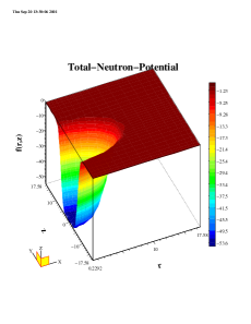
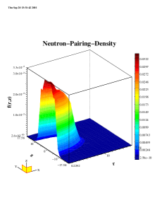
Figure 1: Neutron potential and pairing density for ${}^{150}Sn$.

In figure 1 we show the total neutron potential and the neutron pairing density. As we can see the pairing effect in the case of ${}^{150}Sn$ is appreciable.

5 Conclusions

We have seen that our calculations are close to the experimental values, and that our two-dimensional, axially symmetric code agrees with the calculations of the one-dimensional HFB code [4] for spherical nuclei.

The axial symmetry imposed in our HFB code is expected to be well suited in describing deformed nuclei far from stability. Our HFB approach for such nuclei works especially well in treating strong coupling to the continuum, which was shown to be crucial for obtaining convergence.

References

- [1] “Scientific Opportunities with an Advanced ISOL Facility”, Panel Report (Nov. 1997), ORNL
- [2] “RIA Physics White Paper”, RIA 2000 Workshop, Raleigh-Durham, NC (July 2000), distributed by NSCL, Michigan State University
- [3] J. Dobaczewski, H. Flocard, and J. Treiner, Nucl. Phys. A422 (1984) 103.
- [4] J. Dobaczewski, W. Nazarewicz, T.R. Werner, J.F. Berger, C.R. Chinn, and J. Dechargé, Phys. Rev. C53 (1996) 2809.
- [5] P. Ring and P. Schuck, “The Nuclear Many-Body Problem”, Springer Verlag, New York (1980), in particular chapters 6 and 7.
- [6] P.-G. Reinhard, D.J. Dean, W. Nazarewicz, J. Dobaczewski, J. A. Maruhn, and M.R. Strayer, Phys. Rev. C 60, 014316 (1999)
- [7] E. Chabanat, P. Bonche, P. Haensel, J. Meyer, and R. Schaeffer, Nucl. Phys. A 635 (1998) 231; Nucl. Phys. A 643 (1998) 441
- [8] M.V. Stoitsov, J. Dobaczewski, P. Ring, and S. Pittel, Phys. Rev. C 61, 034311 (2000)
- [9] V.E. Oberacker and A.S. Umar, in “Perspectives in Nuclear Physics” (ed. J.H. Hamilton, H.K. Carter and R.B. Piercey), World Scientific Publ. Co. (1999), p. 255-266.
- [10] D.R. Kegley, V.E. Oberacker, M.R. Strayer, A.S. Umar, and J.C. Wells, J. Comp. Phys. 128 (1996) 197.
- [11] D.R. Kegley, Ph.D. thesis, Vanderbilt University (1996)
- [12] J.C. Wells, V.E. Oberacker, M.R. Strayer and A.S. Umar, Int. J. Mod. Phys. C6 (1995) 143
- [13] W. Nazarewicz, J. Dobaczewski, T.R. Werner, J.A. Maruhn, P.-G. Reinhard, K.Rutz, C.R. Chinn, A.S. Umar, M.R. Strayer, Phys. Rev. C53, 740 (1996).
- [14] C.R. Chinn, A.S. Umar, M. Vallieres, and M.R. Strayer, Phys. Rev. E50, 5096 (1994).
- [15] A.S. Umar, M.R. Strayer, J.-S. Wu, D.J. Dean, and M.C. Güçlü, Phys. Rev. C44, 2512 (1991).
- [16] E. Terán, V.E. Oberacker, and A.S. Umar, (in preparation).