Radiative corrections in neutrino-deuterium disintegration

Abstract

The radiative corrections of order $\alpha$ for the charged and neutral current neutrino-deuterium disintegration for energies relevant to the SNO experiment are evaluated. Particular attention is paid to the issue of the bremsstrahlung detection threshold. It is shown that the radiative corrections to the total cross section for the charged current reaction are independent of that threshold, as they must be for consistency, and amount to a slowly decreasing function of the neutrino energy $E_{\nu}$, varying from $\sim$ 4% at low energies to $\sim$ 3% at the end of the ⁸B spectrum. The differential cross section corrections, on the other hand, do depend on the bremsstrahlung detection threshold. Various choices of the threshold are discussed. It is shown that for a realistic choice of the threshold, and for the actual electron energy threshold of the SNO detector, the deduced ⁸B $\nu_{e}$ flux should be decreased by $\sim$ 2%. The radiative corrections to the neutral current reaction are also evaluated.

PACS number(s): 13.10.+q, 13.15.+g, 25.30.Pt

I Introduction

Solar neutrinos from ⁸B decay have been detected at the Sudbury Neutrino Observatory (SNO) [1] via the charged current (CC) reaction

$$\nu_{e}+d\rightarrow p+p+e^{-}~{}.$$ (1)

In the next phase of the SNO experiment, currently underway, the rate of the neutral current deuteron disintegration (NC)

$$\nu_{e}+d\rightarrow p+n+\nu_{e}~{}$$ (2)

will be also measured.

From the measurement of the CC reaction rate the flux at Earth of the ⁸B solar $\nu_{e}$ was determined to be [1],

$$\Phi_{SNO}^{CC}(\nu_{e})=1.75\pm 0.07({\rm stat})_{-0.11}^{+0.12}({\rm syst})\pm 0.05({\rm theor})\times 10^{6}{\rm cm}^{-2}{\rm s}^{-1}~{}.$$ (3)

The ⁸B solar neutrinos were also detected in the precision measurement by the Super-Kamiokande Collaboration (SK) [2] using the elastic scattering (ES) on electrons. That reaction is sensitive not only to the charged current weak interaction but also to the neutral current interaction. From the SK measurement the ⁸B solar neutrino flux was deduced to be

$$\Phi_{SK}^{ES}(\nu_{e})=2.32\pm 0.03({\rm stat})_{-0.07}^{+0.08}({\rm syst})\times 10^{6}{\rm cm}^{-2}{\rm s}^{-1}~{}.$$ (4)

The difference between these two flux determinations, at the 3.3 $\sigma$ level, can be regarded as a ‘smoking gun’ proof of neutrino oscillations, independent of the solar model flux calculation. By itself, $\nu_{e}e$ NC scattering cannot account for the difference between (3) and (4). The excess ES events must involve a neutrino species which contributes disproportionately to the NC rate. According to the oscillation hypothesis, some of the ⁸B solar $\nu_{e}$ oscillate into another active neutrino flavor $\nu_{\mu\tau}$. These $\nu_{\mu\tau}$ neutrinos then cannot cause the charged current reaction, Eq.(1), but they can and do undergo NC scattering on electrons. Assuming that this is what is really happening, one arrives at the total ⁸B solar neutrino flux consistent with the Standard Solar Model [3, 4]. This agreement may be used as a supporting evidence for the oscillation hypothesis, which will be further tested by comparing the CC and NC reaction rates measured by the SNO experiment alone.

The goal of the present work is the evaluation of the radiative (order $\alpha$) corrections to the cross sections of the CC and NC reactions. Precise knowledge of these cross sections has obvious relevance for the determination of the ⁸B neutrino flux. Experimentally, one measures the number and energies of the electron events for the CC reaction, or the number of neutron events for the NC reaction, which after corrections for cuts and experimental efficiencies, is an integral over the incoming neutrino energies of the ⁸B solar neutrino flux (possibly modified by the neutrino oscillations) times the differential cross section. Hence any error in the cross section causes a corresponding error in the deduced flux.

In analyzing the SNO CC data the theoretical cross section of Ref. [5] was used. The assumed uncertainty of the calculated cross section is reflected in the theoretical uncertainty of the deduced flux, Eq.(3). However, radiative corrections were not applied to the CC cross section.

The radiative corrections to the CC reaction (1) were evaluated by Towner [6]. That analysis was recently questioned by Beacom and Parke[7], who noted that the total CC cross section for detected and undetected bremsstrahlung differ, according to the analysis of Ref. [6]. Such a difference is unphysical. The observation of Ref. [7] has lead to understandable confusion among experimentalists as to the appropriate radiative corrections to apply to the SNO data. While the published SNO result did not include any radiative corrections, the level of confidence in future CC/NC comparisons could depend significantly on a proper treatment of the radiative corrections. Thus, in what follows we revisit the analysis of Ref. [6], in an effort to resolve the present controversy.

While we have no quarrel with the basic treatment of the radiative corrections to the CC reaction in [6], we confirm the observations of Ref. [7] and identify the origins of the inconsistency in Towner’s results: (a) neglect of a strong momentum-dependence in the Gamow-Teller ³S${}_{1}\to^{1}$S₀ matrix element, and (b) improper ordering of limits involving $E_{\gamma}^{min}$ and the infrared regulator. After correcting for these issues, we obtain identical total CC cross sections for detected and undetected bremsstrahlung. The results imply an $E_{\nu}$-dependent correction to the total CC cross section which varies from $\sim 4\%$ to $\sim 3\%$ over the range of available neutrino energies.

In addition to foregoing, we also recast the treatment in Ref. [6] of hadronic effects in the radiative corrections into the language of effective field theory (EFT). Although the traditional treatment in Ref. [8] and EFT frameworks are equivalent, the latter provides a systematic approach for long-distance, hadronic effects presently uncalculable from first principles in QCD. As discussed in Ref. [8], matching the asymptotic and long-distance calculations (in EFT) involves use of a hadronic scale, $M_{had}$, whose choice introduces a small theoretical uncertainty into the radiative corrections. We argue that the choice of $M_{had}$ made in Ref. [6] is possibly inappropriate for the process at hand, and attempt to quantify the uncertainty associated with the choice of an appropriate value. Given the SNO experimental error, this theoretical uncertainty is unlikely to affect the interpretation of the CC results. It may, however, be relevant to future, more precise determinations of Gamow-Teller transitions in other contexts.

Finally, for completeness, we revisit the analysis of the NC radiative correction computed in Ref. [6]. In this case, bremsstrahlung contributions are highly suppressed, the correction is governed by virtual gauge boson exchange, and the result is esssentially $E_{\nu}$-independent. We obtain a correction to the NC cross section that is a factor of four larger than given in Ref. [6], which neglected the dominant graph. The implication of a complete analysis is the application of a $\sim 1.5\%$ correction to the tree-level NC cross section.

Our discussion of these points is organized in the remainder of the paper as follows. In Section II we present our formalism for the CC radiative corrections. Given the thorough discussion of this formalism in Ref. [6], we restrict ourselves to only brief explanation of the basic formalism that is used to evaluate the corresponding Feynman graphs and deduce the formulae for the differential cross section. In Section III we discuss the delicate issue of bremsstrahlung thresholds and the ‘detector dependence’ of the CC radiative corrections. In particular, we derive the corrections for two extreme cases of very high and very low thresholds, and for an intermediate, more realistic case [9]. We show in Section III where our results disagree with those of Ref. [6], and trace the origin of these discrepancies. Detailed tabular evaluation of the modification of the differential CC cross section for the ‘realistic’ bremsstrahlung threshold is provided as well. In Section IV we consider the effects of the electron spectrum distortion. In particular, we consider the test of the oscillation null hypothesis, where the unperturbed $\nu_{e}$ spectrum of the ⁸B decay is expected. In Section V we derive the corrections to the NC reaction rate and discuss the differences with their treatment in [6]. We conclude in Section VI. Finally, in Appendix we collect needed formulae for the evaluation of the triple differential cross section (in $E_{e},E_{\gamma}$ and the angle between them) for an arbitrary bremsstrahlung threshold.

II General considerations

In the charged current neutrino disintegration of deuterons at rest in the laboratory frame, Eq.(1), the incoming $\nu_{e}$ energy $E_{\nu}$, corrected for the mass difference $\Delta=M_{d}-2M_{p}=-0.931$ MeV, is shared by the outgoing electron (energy $E_{e}$), the energy of the relative motion of the two protons $p^{2}/M_{p}$, and by the energy of a bremsstrahlung photon $E_{\gamma}$ (if such a photon is emitted), i.e.,

$$E_{\nu}+\Delta=E_{e}+p^{2}/M_{p}+(E_{\gamma})~{}.$$ (5)

This energy conservation condition must be, naturally, always obeyed. For the neutrino energies we are considering the motion of the center of mass of the protons can be neglected.

Since radiative corrections are only few percent in magnitude, we follow Towner [6] and use for the ‘tree level’ differential cross section the formula based on the effective range theory (see [10, 11])

$$\left(\frac{{\rm d}\sigma_{CC}}{{\rm d}E_{e}}\right)_{tree}=\frac{2G_{F}^{2}}{\pi}V_{ud}^{2}g_{A}^{2}M_{p}p_{e}E_{e}p|I(p^{2})|^{2},$$ (6)

where for $p^{2}$ we should substitute $M_{p}(E_{\nu}+\Delta-E_{e})$. It is important to remember that the radial integral, the overlap of the radial wave function of the two continuum protons and the bound state

$$I(p^{2})=\int u_{cont}^{*}(pr)u_{d}(r)dr$$ (7)

also depends on the momentum $p$ of the relative motion of the two protons.

We plot in Fig. 1 the quantity $|I(p^{2})|^{2}$ evaluated as in Ref. [10], i.e., using the scattering length and effective range approximation as well as the Coulomb repulsion of the two final protons. The most important feature of the $p^{2}$ dependence is its width when expressed in the relevant units of $p^{2}/M_{p}$, the kinetic energy of the continuum protons. It is easy to understand the width of the curve as demonstrated in the figure. The dashed line represents the same $|I(p^{2})|^{2}$ evaluated neglecting Coulomb repulsion as well as effective range. In that case a simple analytic expression obtains,

$$|I(p^{2})|^{2}\simeq\frac{const}{(1+a_{pp}^{2}p^{2})(1+\frac{p^{2}}{E_{b}M_{p}})^{2}}~{},$$ (8)

where $E_{b}$ is the deuteron binding energy and the proton-proton scattering length is $a_{pp}$ = -7.82 fm. The value of the proportionality constant is irrelevant in the present context. Thus the width is determined essentially by $\sim(\hbar c)^{2}/(a_{pp}^{2}M_{p})\sim$ 0.7 MeV (the term with $p^{2}/E_{b}M_{p}$ contributes very little to the width) in agreement with the more accurate evaluation. We explain the relevance of this width later, in Section III.

The radiative corrections consist of two components: the exchange of virtual photons and $Z$-bosons and the emission of real bremsstrahlung photons. The Feynman graphs for the exchange of virtual $\gamma$ quanta and $Z$ bosons are shown in Fig. 2. The bremsstrahlung graps are shown in Fig. 3. The photon emission by the moving electron is dominant ( graph (b) in Fig. 3), but the complete set of graphs must be considered for gauge invariance. The treatment of radiative corrections proceeds along the well tested lines developed for the treatment of beta decay (see Ref. [8] for a review).

Let us consider the virtual exchange corrections first. While the treatment of corrections involving only leptons is straightforward, those involving hadronic participants require considerable care. To that end, it is useful to adopt the framework of an EFT, valid below a scale $\mu\sim 1$ GeV. Long-distance physics ($p\lesssim\mu$) associated with non-perturbative strong interactions are subsumed into hadronic matrix elements of appropriate hadronic operators. Short distance physics ($p\gtrsim\mu$) contributions are contained in coefficient functions $C(\mu)$ multiplying the effective operators (see, e.g., the discussion in Ref. [12]). In the present case, the CC reaction of Eq. (1) is dominated by the pure Gamow-Teller transition ³S${}_{1}\to^{1}$S₀. Thus, for the low-energy EFT, we require matrix elements of the effective, hadronic axial current. The resulting CC amplitude is

$$M(^{3}{S}_{1}\to^{1}{S}_{0})=-{G_{F}\over\sqrt{2}}V_{ud}{\bar{e}}\gamma_{\lambda}(1-\gamma_{5})\nu C(\mu)\langle^{1}{S}_{0}|{\tilde{A}}^{\lambda}|^{3}{S}_{1}\rangle+\cdots\ \ ,$$ (9)

where $C(\mu)$ is the short-distance coefficient function mentioned above; ${\tilde{A}}^{\lambda}$ is an effective, isovector axial current operator built out of low-energy degrees of freedom (e.g., nucleon and pion fields); the $+\cdots$ denote contributions from higher-order effective operators; and where the $\mu$-dependence of $C(\mu)$ compensates for that of the axial current matrix element, leading to a $\mu$-independent result. In effect, the presence of $C(\mu)$ is needed for matching of the effective theory onto the full theory (QCD plus the electroweak Standard Model).

Note that we have normalized the amplitude to the Fermi constant determined from the muon lifetime, $G_{F}=1.16639(5)\times 10^{-5}$ GeV^-2 [13]. Thus, $C(\mu)$ contains the difference

$$\Delta r_{\beta}^{A(p\geq\mu)}-\Delta r_{\mu}\ \ ,$$ (10)

where $\Delta r_{\beta}^{A(p\geq\mu)}$ contains the short distance virtual corrections to the axial vector semileptonic amplitude and $\Delta r_{\mu}$ denotes the Standard Model electroweak radiative corrections to the muon decay amplitude. In the difference (10), all universal short-distance effects (Fig. 2a-c) cancel, leaving only contributions from the non-universal parts of diagrams in Fig. 2b-d.

As a corollary, we emphasize that care must be exercised in choosing a value for the axial coupling constant $g_{A}$ used in computing $\langle^{1}{S}_{0}|{\tilde{A}}^{\lambda}|^{3}{S}_{1}\rangle$. Typically, $g_{A}$ is determined from the experimental ratio [14]

$$\lambda={G_{A}^{\prime}\over G_{V}^{\prime}}={G_{A}(1+\Delta r_{\beta}^{A})\over G_{V}(1+\Delta r_{\beta}^{V})}\approx{G_{A}\over G_{V}}(1+\Delta r_{\beta}^{A}-\Delta r_{\beta}^{V})\ ,$$ (11)

where $\Delta r_{\beta}^{V}$ ($\Delta r_{\beta}^{A}$) denotes the total radiative correction to the vector (axial vector) semileptonic amplitude. The CVC relation implies $G_{V}=G_{F}V_{ud}$, while the axial coupling constant is defined via $G_{A}=g_{A}G_{F}V_{ud}$. To the extent that $\Delta r_{\beta}^{V}=\Delta r_{\beta}^{A}$, the ratio $\lambda$ is just $g_{A}$. As we note below, however, hadronic contributions to $\Delta r_{\beta}^{V}$ and $\Delta r_{\beta}^{A}$ are in general not identical. While we speculate that the differences are considerably smaller than relevant here, arriving at a reasonable estimate requires a future, more systematic study.

The asymptotic (short-distance) contributions to $C(\mu)$ have been computed in Ref. [8] using current algebra techniques and the short-distance operator product expansion. The result implies

$$C(\mu)=1+{\alpha\over 2\pi}\left[3{\bar{Q}}\ln\frac{M_{Z}}{\mu}+\frac{3}{2}\ln\frac{M_{Z}}{\mu}+\frac{1}{2}{\cal A}_{g}(\mu)\right]+b(\mu)\ \ ,$$ (12)

where ${\bar{Q}}$ is the average charge of the quarks involved in the transition

$${\bar{Q}}=\frac{1}{2}(Q_{u}+Q_{d})=\frac{1}{6}\ \ ,$$ (13)

${\cal A}_{g}(\mu)$ contains short-distance QCD corrections, and $b(\mu)$ must be included to correct for any mismatch between the $\mu$-dependence appearing elsewhere in $C(\mu)$ and that appearing in the matrix element of ${\tilde{A}}_{\lambda}$. Explicit expressions for the short-distance QCD contributions ${\cal A}_{g}(\mu)$ may be found in Ref. [8]. We note that the second term of Eq. (12) ($\propto{\bar{Q}}$) arises from the sum of box diagrams involving $(\gamma,W)$ and $(Z,W)$ pairs, while the third term arises from QED external leg and vertex corrections. When long-distance, ${\cal O}(\alpha)$ virtual effects arising from the matrix elements in Eq. (9) are included along with those appearing in $C(\mu)$, the $\mu$-dependence of the third term in Eq. (12) cancels completely.

Long-distance virtual photon contributions also contain an infrared singularity which is conventionally regulated by including a photon “mass” $\lambda$. The resulting $\lambda$-dependence is cancelled by corresponding $\lambda$-dependence in the bremsstrahlung cross section, yielding a $\lambda$-independent correction to the total CC cross section. In what follows, then, it is convenient to consider the ${\cal O}(\alpha)$ correction to the tree-level cross section:

$$d\sigma_{CC}=d\sigma_{CC}^{tree}\left[1+\frac{\alpha}{\pi}g\right]~{},$$ (14)

where the correction factor $g$ depends on $E_{\nu}$ and $E_{e}$ as well as on $E_{\gamma}$ when bremsstrahlung photons are detected. This function receives contributions from $C(\mu)$,

$$\frac{\alpha}{\pi}g_{v}^{p\gtrsim\mu}=2\left[C(\mu)-1\right]\ ,$$ (15)

long-distance ($p\lesssim\mu$) virtual contributions to the the axial current matrix element in Eq. (9), $g_{v}^{p\lesssim\mu}$, and the bremsstrahlung differential cross section, $g_{b}$.

In the analysis of Ref. [6], the long-distance contributions arising from virtual processes is obtained by treating the nucleon as a point-like, relativistic particle. The result is

$$g_{v}^{p\lesssim\mu} = \frac{3}{2}{\rm ln}\left(\frac{\mu}{M_{p}}\right)+3{\bar{Q}}{\rm ln}\left(\frac{\mu}{M_{A}}\right)+{\cal A}-\frac{3}{8}$$ (16)

$${\cal A} = \frac{1}{2}\beta{\rm ln}\left(\frac{1+\beta}{1-\beta}\right)-1+2{\rm ln}\left(\frac{\lambda}{m_{e}}\right)\left[\frac{1}{2\beta}{\rm ln}\left(\frac{1+\beta}{1-\beta}\right)-1\right]$$ (18)

$$+\frac{3}{2}{\rm ln}\left(\frac{M_{p}}{m_{e}}\right)-\frac{1}{\beta}\left[\frac{1}{2}{\rm ln}\left(\frac{1+\beta}{1-\beta}\right)\right]^{2}+\frac{1}{\beta}L\left(\frac{2\beta}{1+\beta}\right)~{}.$$

Here, $L$ is the Spence function and the $-3/8$ is added to obtain agreement with the $\beta$-decay correction [8] and neutrino capture reaction $\bar{\nu_{e}}+p\rightarrow e^{+}+n$ as calculated in Refs. [15, 16]. Note that when this $-3/8$ is added to ${\cal A}$, the resulting expression agrees with the calculations of Refs. [8, 15, 16].

We observe that the sum $g_{v}^{p\gtrsim\mu}+g_{v}^{p\lesssim\mu}$ is independent of $M_{p}$. It does, however, contain the logarithm

$$3{\bar{Q}}\ln\frac{M_{Z}}{M_{A}}$$ (19)

where $M_{A}$ has been chosen in Ref. [6] as a hadronic scale associated with the long-distance part of the $(W,\gamma)$ box diagram. Neglecting terms proportional to $E_{e}$ and $m_{e}$, the sum of the box and crossed-box diagrams depends on the antisymmetric T-product of currents

$$\epsilon_{\mu\nu\lambda\rho}\int\ d^{4}xe^{ik\cdot x}\langle^{1}{S}_{0}|T[J^{\lambda}_{EM}(x)J^{\rho}_{CC}(0)]|^{3}{S}_{1}\rangle\ \ \ ,$$ (20)

where $J^{\lambda}_{EM}$ and $J^{\rho}_{CC}$ denote the electromagnetic and weak charged currents, respectively, and where the $\mu$ and $\nu$ indices are contracted with loop momentum and the lepton current. In order that the antisymmetric T-product appearing in Eq. (20) produce a Gamow-Teller transition, only the vector current part of $J^{\rho}_{CC}$ must be retained. In contrast, for pure Fermi transitions as considered in Ref. [8], only the axial vector charged current operator contributes. In that work, a choice for the hadronic scale was made based by considering $\pi$ $\beta$-decay (a pure Fermi transition), and a vector meson dominance model for the axial vector charged current operator, leading to the appearance of the $a_{1}$ meson mass $M_{A}$ as the long-distance hadronic scale.

In the present case, such a choice appears inappropriate, since the relevant current operator is a vector, rather than axial vector current. To the extent that the vector meson dominance picture is as applicable to nucleons as to pions, a more reasonable choice for the hadronic scale would be $m_{\rho}$. However, such a choice is unabashedly model-dependent and calls for some estimate of the theoretical uncertainty. On general grounds, it is certainly reasonable to choose a hadronic scale anywhere between the chiral scale $\Lambda_{\chi}=4\pi F_{\pi}\approx$ 1.17 GeV and $\Lambda_{QCD}\approx$ 200 MeV. Indeed, the latter choice could arise naturally from $\Delta$-intermediate state contributions to the $(W,\gamma)$ box diagrams. Thus, we replace the logarithm in Eq. (19)

$$3{\bar{Q}}\ln\frac{M_{Z}}{M_{had}}=2.39_{-.21}^{+.67}\ ,$$ (21)

where the central value corresponds to $M_{had}=m_{\rho}$; the upper value corresponds to $M_{had}=\Lambda_{QCD}$; and the lower value is obtained with $M_{had}=\Lambda_{\chi}$. This range corresponds to a spread of 0.2% in predictions for the cross section . While this uncertainty is too small to affect the determination of the ⁸B neutrino flux, it could affect more precise determinations of Gamow-Teller transitions for other purposes.

The choice of $M_{had}$ amounts to use of a model for $b(\mu)$. A source of potentially larger theoretical uncertainties lies in possible additional, model-dependent contributions to this constant. While a complete study of these effects goes beyond the scope of the present work, we observe that the hadronic uncertainty cannot be finessed away using, e.g., chiral perturbation theory, since we have no independent measurements from which to fix the relevant low-energy constants. Moreover, the $\mu$-dependence introduced through the short-distance QCD correction ${\cal A}_{g}(\mu)$ must be cancelled by a corresponding $\mu$-dependent term in $b(\mu)$. To date, no calculation has produced such a cancellation. While the effect of this uncorrected mismatch between short- and long-stance effects is likely to be small, we are unable to quantify it at the present time.

In contrast to the virtual corrections, the bremsstrahlung correction $g_{b}$ is relatively free from hadronic uncertainties. In order to evaluate the bremsstrahlung part, one has to add, in principle, the contribution of all graphs with photon lines attached to all external charged particles. Only the sum of these graphs is gauge-invariant. However, for the low energies, the electron bremsstrahlung dominates over the proton, deuteron, and $W$ bremsstrahlung.

Writing again the correction to the cross section in the form $1+\alpha/\pi g_{b}(E_{e},E_{\nu})$ one obtains the differential bremsstrahlung correction in the form

$$\frac{{\rm d}g_{b}(E_{e},E_{\nu},k)}{{\rm d}k} = \left[\frac{E_{\nu}+\Delta-E_{e}-E_{\gamma}}{E_{\nu}+\Delta-E_{e}}\right]^{1/2}\frac{k^{2}}{2E_{\gamma}}$$ (22)

$$\times \int_{-1}^{+1}{\rm d}x\left[\frac{E_{\gamma}}{E_{e}^{2}(E_{\gamma}-\beta kx)}+\beta^{2}\frac{E_{e}+E_{\gamma}}{E_{e}}\frac{1-k^{2}x^{2}/E_{\gamma}^{2}}{(E_{\gamma}-\beta kx)^{2}}\right]~{},$$ (23)

where $k$ is the photon momentum, and $E_{\gamma}=(k^{2}+\lambda^{2})^{1/2}$, i.e. $\lambda$ is as before the ‘photon mass’. Also, $x=\cos(\theta_{e,\gamma})$.

The dependence on the ‘photon mass’ $\lambda$ is eliminated only when one adds to the $\lambda$ dependent part of the virtual correction $\cal A$ an integral over the bremsstrahlung spectrum up to some $E_{\gamma}^{min}\gg\lambda$. We will discuss the various possible choices of $E_{\gamma}^{min}$ in the next section, but here as an example we evaluate one of the integrals that appears in that context

$$\int_{0}^{E_{\gamma}^{min}}\frac{k^{2}{\rm d}k}{\sqrt{\lambda^{2}+k^{2}}}\int_{-1}^{+1}\frac{{\rm d}x}{(E_{\gamma}-\beta kx)^{2}}=2\int_{0}^{E_{\gamma}^{min}}\frac{k^{2}{\rm d}k}{\sqrt{\lambda^{2}+k^{2}}(\lambda^{2}+m_{e}^{2}/E_{e}^{2}k^{2})}$$ (24)

$$= 2\frac{E_{e}^{2}}{m_{e}^{2}}\left[\int_{0}^{E_{\gamma}^{min}}\frac{{\rm d}k}{\sqrt{\lambda^{2}+k^{2}}}-\int_{0}^{E_{\gamma}^{min}}\frac{\lambda^{2}{\rm d}k}{\sqrt{\lambda^{2}+k^{2}}(\lambda^{2}+m_{e}^{2}/E_{e}^{2}k^{2})}\right]$$ (25)

$$= 2\frac{E_{e}^{2}}{m_{e}^{2}}\left[{\rm ln}\frac{2E_{\gamma}^{min}}{\lambda}-\frac{1}{2\beta}{\rm ln}\left(\frac{1+\beta}{1-\beta}\right)\right]~{},$$ (26)

where $\beta=p_{e}/E_{e}$ and the last integral, which is independent of $E_{\gamma}^{min}$, was evaluated after the substition $z=k/\lambda$ in the limit $E_{\gamma}^{min}/\lambda\rightarrow\infty$. One must not use the limit $E_{\gamma}^{min}\rightarrow 0$ before all terms containing $\lambda$ are eliminated.

To evaluate the full radiative correction, we assume that in an experiment one measures the number of events with energy $E_{obs}\pm{\rm d}E_{obs}$. Here $E_{obs}=E_{e}$ when the bremsstrahlung photon (if such a photon is emitted) has energy of less than $E_{\gamma}^{min}$. We will also assume that when $E_{\gamma}\geq E_{\gamma}^{min}$ then $E_{obs}=E_{e}+E_{\gamma}$. (In the next section we will also consider a modification to the latter rule, making it closer to the actual conditions of the SNO experiment [9].)

Thus the radiative correction to the cross section can be expressed as

$$\left(\frac{{\rm d}\sigma_{CC}}{{\rm d}E_{obs}}\right)_{rad}=\frac{\alpha}{\pi}\left[g_{v}+g_{b}^{low}(E_{\gamma}<E_{\gamma}^{min})+g_{b}^{high}(E_{\gamma}\geq E_{\gamma}^{min})\right]~{}.$$ (27)

We describe in the next section how to evaluate these three functions in general and for three particular choices of $E_{\gamma}^{min}$.

III Radiative corrections to the CC cross section

Treatment of radiative corrections involving virtual photon exchange as well as bremsstrahlung photon emission is a delicate issue due to the appearence of infrared divergencies. In our analysis we follow the conventional approach of introducing infrared regulator in the form of photon mass $\lambda$, and split the bremsstrahlung contributions into two pieces below and above the threshold value $E_{\gamma}^{min}$ as explained above. When contribution from virtual photon exchange are added to the piece with $E_{\gamma}<E_{\gamma}^{min}$, the dependence on infrared regulator $\lambda$ is eliminated. However, it is effectively replaced by a dependence on $E_{\gamma}^{min}$.

The threshold $E_{\gamma}^{min}$ is a detector-dependent quantity, and may vary depending on the experimental conditions. In addition, the experimental conditions also dictate how to combine the piece with $E_{\gamma}<E_{\gamma}^{min}$ ( $g_{v}+g_{b}^{low}$) and the $E_{\gamma}>E_{\gamma}^{min}$ part. Thus it is impossible to give a completely general recipe here.

With this caveat in mind, in our analysis we adopt a following framework. Each detected CC event is characterized by the recorded energy $E_{obs}$ which in general is a function of electron energy $E_{e}$ and, if present, photon energy $E_{\gamma}$: $E_{obs}={E_{obs}}(E_{e},E_{\gamma})$. In the following we concentrate in particular on the role played in this context by the threshold $E_{\gamma}^{min}$.

We consider the following situations:

A) The electrons are always recorded above the electron detection threshold $E_{e}^{min}$, and the bremsstrahlung photons are never detected, i.e. $E_{\gamma}^{min}\rightarrow\infty$.

B) The electrons are always recorded above the electron detection threshold $E_{e}^{min}$, and the bremsstrahlung photons are also always detected, i.e. $E_{\gamma}^{min}\rightarrow 0$.

C) A more realistic case, resembling the actual situation in the SNO detector [9] when only part of the $E_{\gamma}$ energy is recorded, namely $E_{obs}=(E_{e}-m_{e})\theta(E_{e}-E_{e}^{min})+m_{e}+(E_{\gamma}-E_{\gamma}^{min})\theta(E_{\gamma}-E_{\gamma}^{min})$. Here $\theta(x)$ is the step function.

We simplify the cases A) and B) even further by considering an idealized detector with $E_{e}^{min}=m_{e}$, i.e. all electrons and, thus, all neutrino interaction events are detected. When integrated over $E_{obs}$ one arrives at the total number of events caused by a neutrino of energy $E_{\nu}$. That quantity must be, naturally, independent on the bremsstrahlung threshold $E_{\gamma}^{min}$. This is the consistency requirement imposed by Beacom and Parke [7]. We verify that our results fulfill this condition.

In Fig. 4 we plot as an example the normalized radiative correction to the differential cross-section ${{\delta d\sigma(E_{\nu},E_{obs})}\over{dE_{obs}}}/{\sigma_{tot}^{tree}(E_{\nu})}$ for $E_{\nu}$ = 10 MeV and two extreme cases $E_{\gamma}^{min}\rightarrow\infty$ (bremsstrahlung never detected, full line) and $E_{\gamma}^{min}\rightarrow 0$ (bremsstrahlung always detected, dashed line). The two corresponding curves are quite different, reflecting the different dependence of $E_{obs}$ on $E_{e}$ and $E_{\gamma}$. However, the areas under the curves are equal as they must for consistency.

It is interesting to note that evaluation by Towner [6] considers the same limiting cases. However, the results of Ref. [6] give different corrections to the total cross section, $\delta\sigma^{tot}$, i.e. they fail the consistency check. In fact, our results and Ref. [6] differ in both extremes. We trace now the origin of these discrepancies.

A The case of $E_{\gamma}^{min}\rightarrow\infty$, no bremsstrahlung detected

Let us first consider the limit $E_{\gamma}^{min}\rightarrow\infty$. In that case we have to integrate the bremsstrahlung spectrum over the photon momentum from $0\rightarrow\infty$. At the same time, the energy conservation condition, Eq. (5), must be obeyed. Since now $E_{obs}\equiv E_{e}$, then for a fixed $E_{\nu}+\Delta-E_{e}$ the quantity $p^{2}/M_{p}$ must be varied together with $E_{\gamma}$. As noted above, and illustrated in Fig. 1, the quantity $|I(p^{2}/M_{p})|^{2}$ is a rapidly varying function which falls off quickly for $p^{2}/M_{p}\geq$ 0.7 MeV. Therefore to correctly account for this dependence we write

$$\left(\frac{{\rm d}\sigma_{CC}}{{\rm d}E_{e}}\right)_{b}={\alpha\over\pi}\left(\frac{{\rm d}\sigma_{CC}}{{\rm d}E_{e}}\right)_{tree}\int_{0}^{E_{\gamma}^{min}}{{|I(E_{\nu}+\Delta-E_{e}-E_{\gamma}^{k})|^{2}}\over{|I(E_{\nu}+\Delta-E_{e})|^{2}}}\frac{{\rm d}g_{b}(E_{e},E_{\nu},k)}{{\rm d}k}dk,$$ (28)

where $g_{b}(E_{e},E_{\nu},k)$ is given in Eq. (22). If $|I(E_{\nu}+\Delta-E_{e}-E_{\gamma})|^{2}$ could in fact be treated as a constant, the ratio of the two $I^{2}$ would be unity, and Eq. (28) would be identical to Eq. (13) in [6]. To make the connection with Ref. [6] even more concrete we write (note that for $E_{\gamma}<E_{\gamma}^{min}$, $E_{obs}=E_{e}$):

$$\left(\frac{{\rm d}\sigma_{CC}}{{\rm d}E_{obs}}\right)_{b} = \left(\frac{{\rm d}\sigma_{CC}}{{\rm d}E_{obs}}\right)_{b}^{[Towner]}+{\alpha\over\pi}\left(\frac{{\rm d}\sigma_{CC}}{{\rm d}E_{obs}}\right)_{tree}$$ (29)

$$\times \int_{0}^{E_{\gamma}^{min}}\left({{|I(E_{\nu}+\Delta-E_{obs}-E_{\gamma}^{k})|^{2}}\over{|I(E_{\nu}+\Delta-E_{obs})|^{2}}}-1\right)\frac{{\rm d}g_{b}(E_{obs},E_{\nu},k)}{{\rm d}k}dk~{}.$$ (30)

(In Eqs. (28,29) the upper limit of the integral obviously should not extend beyond the corresponding bremssstrahlung endpoint.)

The first term on the r.h.s of Eq. (29) is the contribution present in Ref. [6]. It contains infrared divergence that disappears after contributions from virtual photons are added. The second term is infrared finite. Due to the shape of $|I(E_{\nu}+\Delta-E_{e}-E_{\gamma}^{k})|^{2}$ this term enhances the contribution of the low energy tail in $({\rm d}\sigma_{CC}/{\rm d}E_{obs})_{b}$. The overall result of the low $E_{obs}$ tail enhancement is that the total cross-section is increased by about 3% compared to corresponding result in [6] for the considered case of $E_{\nu}$ = 10 MeV.

B The case $E_{\gamma}^{min}\rightarrow 0$, bremsstrahlung always detected

If one wants to study the opposite extreme $E_{\gamma}^{min}\rightarrow 0$ it is crucial in Eq. (27) to first add all three terms, eliminate infrared cutoff dependence, and only then take the limit $E_{\gamma}^{min}\rightarrow 0$. The order of limits $\lambda\rightarrow 0$ and $E_{\gamma}^{min}\rightarrow 0$ is important because upper limit of integrals like Eq. (24) is $E_{\gamma}^{min}/{\lambda}$. Since $\lambda$ ultimately is an infinitesimal unphysical parameter it is mandatory to maintain $E_{\gamma}^{min}\gg\lambda$ during the entire course of the calculation . This leads to a non-intuitive result that the second term in Eq. (27) has a non-zero contribution even in the limit $E_{\gamma}^{min}\rightarrow 0$. In particular, one must write the following expression corresponding to the second term on the r.h.s of Eq. (27), i.e. for $E_{\gamma}\leq E_{\gamma}^{min}$:

$$\left(\frac{{\rm d}\sigma_{CC}}{{\rm d}E_{obs}}\right)_{b}=\left(\frac{{\rm d}\sigma_{CC}}{{\rm d}E_{obs}}\right)_{tree}{{\alpha}\over{\pi}}\left(2\ln\left({{E_{\gamma}^{min}}\over{\lambda}}\right)\left[\frac{1}{2\beta}\ln\left(\frac{1+\beta}{1-\beta}\right)-1\right]+{\cal C}(\beta)\right)+{\cal O}(E_{\gamma}^{min})$$ (31)

with

$${\cal C}(\beta)=2\ln(2)\left[\frac{1}{2\beta}\ln\left(\frac{1+\beta}{1-\beta}\right)-1\right]+1+\frac{1}{4\beta}\ln\left(\frac{1+\beta}{1-\beta}\right)$$ (32)

$$\times\left[2+\ln\left({{1-\beta^{2}}\over 4}\right)\right]+{1\over{\beta}}\left[{L(\beta)-L(-\beta)}\right]+{1\over 2\beta}\left({L\left({{1-\beta}\over{2}}\right)-L\left({{1+\beta}\over{2}}\right)}\right)~{},$$ (33)

where for $\beta<1$ the Spence function is

$$L(\beta)=\int_{0}^{\beta}{{\ln(|1-x|)}\over x}dx=-\sum_{k=1}^{\infty}\frac{\beta^{k}}{k^{2}}~{}.$$ (34)

The $\lambda$-dependent terms in Eq. (31) will be cancelled by $\lambda$-dependent pieces from virtual photon contributions, and the logarithmic divergence in $E_{\gamma}^{min}$ will disappear after the piece with $E_{\gamma}>E_{\gamma}^{min}$ is added to the cross-section (third term in Eq. (27)). Only after this is done is one allowed to take $E_{\gamma}^{min}\rightarrow 0$. The most striking feature of Eq. (32) is that it is independent of $E_{\gamma}^{min}$. Consequently, it survives in the limit $E_{\gamma}^{min}\rightarrow 0$. It appears that this procedure was not followed in Ref. [6] and, therefore, equation (44) and Table II in [6] must be modified accordingly. We plot in Fig. 5 the cross section correction $(\alpha/\pi)g(E_{obs})$, which is for $E_{\gamma}^{min}\rightarrow 0$ independent of the neutrino energy $E_{\nu}$. Note that it differs in slope compared with its analog in Table II of Ref. [6].

The two aforementioned modifications to the treatment in Ref. [6] allowed us to bring the two cases $E_{\gamma}^{min}\rightarrow\infty$ and $E_{\gamma}^{min}\rightarrow 0$ in agreement in terms of correction to the total cross-section and resolve the discrepancy mentioned in Ref. [7]. In either of these extreme cases, by integrating over $E_{obs}$ we obtain the QED correction to the total cross section as a function of the neutrino energy $E_{\nu},~{}\delta\sigma^{tot}(E_{\nu})$, displayed in Fig. 6.

C Realistic bremsstrahlung threshold

The treatment of the more realistic case is now straightforward. First and second terms (virtual and $E_{\gamma}<E_{\gamma}^{min}$) on the r.h.s of Eq. (27) are evaluated by setting $E_{\gamma}^{min}=1$ MeV [9] and $E_{e}=E_{obs}$. In the third term one has to set $E_{\gamma}+E_{e}=E_{obs}+E_{\gamma}^{min}=\rm const$ and integrate over $E_{e}$.

In particular, suppose we write the double differential cross-section for the $d+\nu_{e}\rightarrow p+p+e+\gamma$ as $d^{2}\sigma_{CC}^{\gamma}/(dE_{e}dE_{\gamma})=f(E_{e},E_{\gamma})$. Then the total cross-section with $E_{\gamma}>E_{\gamma}^{min}$ MeV is:

$$\left(\sigma_{CC}^{\gamma}\right)_{tot}= {\int}_{m_{e}}^{E_{\nu}+\Delta}dE_{e}{\int}_{E_{\gamma}^{min}}^{E_{\nu}+\Delta-E_{e}}f(E_{e},E_{\gamma})dE_{\gamma}$$ (35)

$$= {\int}_{m_{e}}^{E_{\nu}+\Delta-E_{\gamma}^{min}}dE_{obs}{\int}_{m_{e}}^{E_{obs}}f(E_{e},E_{obs}+E_{\gamma}^{min}-E_{e})dE_{e}~{}.$$ (36)

We simply performed the change of integration variables from $(E_{e},E_{\gamma})$ to $(E_{obs},E_{e})$ in the spirit of Ref. [6]. Now we can write in the notation of Eq. (27):

$${\alpha\over\pi}g_{b}^{high}(E_{\gamma}\geq E_{\gamma}^{min})={\int}_{m_{e}}^{E_{obs}}f(E_{e},E_{obs}+E_{\gamma}^{min}-E_{e})dE_{e}~{}.$$ (37)

The result, as expected, is a function of $E_{obs}$ only. In order to generalize to the case $E_{e}^{min}>m_{e}$ one has to be careful because change of variables from $(E_{e},E_{\gamma})$ to $(E_{obs},E_{e})$ becomes less trivial. It is possible to show, however, that the following relationship holds:

$${\alpha\over\pi}g_{b}^{high}(E_{\gamma}\geq E_{\gamma}^{min},E_{e}^{min}>m_{e})={\alpha\over\pi}g_{b}^{high}(E_{\gamma}\geq E_{\gamma}^{min},E_{e}^{min}=m_{e})$$ (38)

$$+ \int_{m_{e}}^{E_{e}^{min}}[f(E_{e},E_{obs}+E_{\gamma}^{min}-m_{e})-f(E_{e},E_{obs}+E_{\gamma}^{min}-E_{e})]dE_{e}~{},$$ (39)

where $f(x,y)$ is the function defined before in Eq. (35). Eq. (38) allows one to obtain the correct spectrum, Eq. (27), for any electron threshold in terms of the ideal case where all electrons are detected. We note that it is only the third term in Eq. (27) that (implicitly) depends on $E_{e}^{min}$. The impact of the refinement in Eq. (38) is rather small for low values of $E_{e}^{min}$. We evaluated it for $E_{e}^{min}=1.5$ MeV (1 MeV kinetic energy). The effect of the second line in Eq. (38) is a 0.03% modification of the differential cross section. Consequently, we neglect this refinement in our analysis.

The spectrum for the case C) is shown in Fig. 4 in the dash-dotted line. As expected, the upper 1 MeV of that spectrum coincides with the $E_{\gamma}^{min}\rightarrow\infty$ case. Note that the areas under all three cases in Fig. 4 are the same, as they must for consistency.

In Table I we provide detailed tabular information on the correction to the differential cross section for the full range of neutrino energies $E_{\nu}$ and $E_{obs}$ for the case C).

IV Folding with the ⁸B spectrum.

In an actual solar neutrino experiment, like SNO, the recorded quantity is the number of events with energy $E_{obs}$ (or the total number of events integrated over $E_{obs}$). This is an integral over the product of the incoming neutrino spectrum and the differential cross section, i.e.

$$\frac{{\rm d}\sigma}{{\rm d}E_{obs}}=\int_{0}^{\infty}\frac{{\rm d}\sigma(E_{\nu})}{{\rm d}E_{obs}}f(E_{\nu}){\rm d}E_{\nu}~{},$$ (40)

where $f(E_{\nu})$ is properly normalized incoming neutrino spectrum, possibly modified by neutrino oscillation. When testing the ‘null hypothesis’, i.e. asking whether neutrinos oscillate, one takes for the incoming neutrino spectrum simply the shape of the $\nu_{e}$ spectrum from ⁸B decay [17] (normalized to unity over the whole range of $E_{\nu}$).

In Fig. 7 we show the folded correction to the differential cross section, Eq. (40) (full line). The case C), i.e. the realistic bremsstrahlung detection threshold has been used to produce the full curve. For comparison we also show similarly folded tree level cross section, scaled by a factor 1/40 so that it fits in the same figure (dashed line). One can see that the two curves are similar in shape which is basically dictated by the incoming ⁸B spectrum, but the QED correction is shifted toward smaller $E_{obs}$, roughly by the value $E_{\gamma}^{min}$ = 1 MeV.

When integrated from the threshold used in the SNO analysis, $E_{obs}^{min}-m_{e}$ = 6.75 MeV, the full line represents $\sim$ 2% increase of the total total cross section, therefore $\sim$ 2% decrease of the deduced flux, Eq. (3), when the radiative corrections are properly included. If it would be possible to reduce the threshold to very low values, the reduction of the flux would be $\sim$ 3%.

These relative increases of the total cross section obviously differ somewhat from the values displayed in Fig. 6 that were obtained for monochromatic neutrinos. The difference is, naturally, caused by the effect of the shape of the radiative correction to the differential cross section in combination with the shape of the ⁸B $\nu_{e}$ spectrum. In particular, for the actual SNO $E_{obs}^{min}$ threshold one could have expected an increase of the cross section (or count rate) due to radiative correction of $\sim$ 3% based on Fig. 6 while the folding with the incoming ⁸B spectrum reduces this value to $\sim$ 2%.

V Radiative corrections to the NC cross section

The NC cross section is governed by the effective four fermion low-energy Lagrangian [18]

$${\cal L}^{\nu-had}=-{G_{F}\over 2\sqrt{2}}{\bar{\nu}}\gamma^{\mu}(1-\gamma_{5})\nu\left[\xi_{V}^{T=1}V_{\mu}^{T=1}+\xi_{V}^{T=0}V_{\mu}^{T=0}+\xi_{A}^{T=1}A_{\mu}^{T=1}+\xi_{A}^{T=0}A_{\mu}^{T=0}\right]\ \ \ ,$$ (41)

where

$$V_{\mu}^{T=1}=\frac{1}{2}\left[{\bar{u}}\gamma_{\mu}u-{\bar{d}}\gamma_{\mu}d\right] V_{\mu}^{T=0}=\frac{1}{2}\left[{\bar{u}}\gamma_{\mu}u+{\bar{d}}\gamma_{\mu}d\right]$$ (42)

$$A_{\mu}^{T=1}=\frac{1}{2}\left[{\bar{u}}\gamma_{\mu}\gamma_{5}u-{\bar{d}}\gamma_{\mu}\gamma_{5}d\right] A_{\mu}^{T=0}=\frac{1}{2}\left[{\bar{u}}\gamma_{\mu}\gamma_{5}u+{\bar{d}}\gamma_{\mu}\gamma_{5}d\right]\ \ \ ,$$ (43)

and where only the effects of up- and down-quarks have been included. At tree level in the Standard Model, one has

$$\xi_{V}^{T=1}=2(1-2\sin^{2}\theta_{W}) \xi_{V}^{T=0}=-4\sin^{2}\theta_{W}$$ (44)

$$\xi_{A}^{T=1}=-2 \xi_{A}^{T=0}=0\ \ \ .$$ (45)

As noted in Ref. [6], the incident and scattered neutrinos do not contribute to the bremsstrahlung cross section at ${\cal O}(G_{F}^{2}\alpha)$, while radiation of real photons from the participating hadrons is negligible. Thus, the dominant radiative corrections involve virtual exchanges, which modify the $\xi_{V,A}^{T}$ from their tree-level values:

$$\xi_{V,A}^{T}\rightarrow\xi_{V,A}^{T}|_{tree}(1+R_{V,A}^{T})\ \ \ ,$$ (46)

where the $R_{V,A}^{T}$ contain the ${\cal O}(\alpha)$ corrections. Since the NC amplitudes are squared in arriving at the cross section, the total correction to the NC cross section will go as twice the relevant $R_{V,A}^{T}$. (In the notation of Ref. [6], $R_{A}^{T=1}=(\alpha/2\pi)g_{v}^{NC}$.)

As emphasized in Ref. [6], considerable simplification follows when one considers only the dominant break-up channel: ³S${}_{1}(T=0)\to^{1}$S${}_{0}(T=1)$. As a $\Delta T=1$, pure spin-flip transition, this amplitude is dominated at low-energies by the Gamow-Teller operator. Magnetic contributions are of recoil order and, thus, $v/c$ suppressed. Consequently, we need retain only the $A_{\mu}^{T=1}$ term in Eq. (41) and consider only the correction $R_{A}^{T=1}$.

The source of corrections to $R_{A}^{T=1}$ include corrections to the $W$ and $Z$-boson propagators (Fig. 8, graph (a)); electroweak and QED vertex corrections to the $Z\nu\nu$ and $Zqq$ couplings (Fig.8, graph (b)); external leg corrections (Fig. 8, graph (c)); and box diagrams involving the exchange of two $W$’s or two $Z$’s (Fig. 8, graph (d)). The presence of $W$-boson propagator corrections arises when the NC amplitude is normalized to the Fermi constant $G_{F}$ determined from muon decay. Only the difference between the gauge boson propagator corrections enters the $R_{V,A}^{T}$ in this case. Note that $Z$-$\gamma$ mixing does not contribute to $R_{A}^{T=1}$ since the neutrino has no EM charge and the photon has no axial coupling to quarks at $q^{2}=0$. Similarly, one encounters no $Z\gamma$ box diagrams for neutrino-hadron scattering.

In the analysis of Ref. [6], only the $ZZ$ box contribution was included, yielding a correction $R_{A}^{T=1}\approx 0.002$. Inclusion of all diagrams, however, produces a substantially larger correction. From the up-dated tabulation of effective $\nu$-$q$ couplings given in Ref. [13], we obtain

$$R_{A}^{T=1}=\rho^{NC}_{\nu N}+\lambda_{dR}-\lambda_{uR}+\lambda_{uL}-\lambda_{dL}-1\approx 0.0077\ ,$$ (47)

where we have followed the notation of Ref. [13]. In particular, the $WW$ box graph contributes roughly 80% of the total:

$$R_{A}^{T=1}(WW-{box})={5\alpha\over 8\pi\sin^{2}\theta_{W}}\approx 0.0063\ .$$ (48)

The net effect of the total correction is therefore $g_{v}^{NC}$ = 6.63, i.e., $\sim 1.5\%$ increase in the NC cross section, as compared to the $0.4\%$ increase quoted in Ref. [6].

VI Conclusions

The radiative correction of order $\alpha$ for the charged and neutral current neutrino-deuterium disintegration and energies relevant to the SNO experiment are consistently evaluated. For the CC reaction the contribution of the virtual $\gamma$ and $Z$ exchange is divided into high and low momentum parts, and the dependence on the corresponding scale $\mu\sim$ 1 GeV separating the two regimes is discussed in detail. For the bremsstrahlung emission we discuss the important role of the bremsstrahlung detection threshold $E_{\gamma}^{min}$. In particular, we consider the two extreme cases $E_{\gamma}^{min}\rightarrow\infty$ and $E_{\gamma}^{min}\rightarrow 0$ as well as a more realistic intermediate case. We show that our treatment, unlike Ref. [6], gives consistent, i.e. $E_{\gamma}^{min}$-independent, correction to the total cross section, shown in Fig. 6. This correction, slowly decreasing with increasing neutrino energy $E_{\nu}$, amounts to $\sim$ 4% at low energies and $\sim$ 3% at the end of the ⁸B spectrum.

The magnitude of this correction is in accord with the correction to the inverse neutron beta decay, $\bar{\nu}_{e}+p\rightarrow n+e^{+}$ evaluated in Refs. [15, 16] and with the correction for the $pp$ fusion reaction evaluated in Ref. [19]. Note that in these references only the ‘outer radiative corrections’, i.e. only the low momentum part of the virtual photon exchange was considered. The high momentum part, which is independent of the incoming or outgoing lepton energies, and which is universal for all semileptonic weak reactions involving $d\leftrightarrow u$ quark transformation, amounts to $\sim$ 2.4% [20] and should be added to the results quoted in Refs. [15, 16, 19].

We identify the origin of the inconsistency of the treatment of Ref. [6]: (a) neglect of a strong momentum-dependence in the Gamow-Teller ³S${}_{1}\to^{1}$S₀ matrix element, which affects the case of $E_{\gamma}^{min}\rightarrow\infty$, and (b) improper ordering of limits involving $E_{\gamma}^{min}$ and the infrared regulator, which affects the case of $E_{\gamma}^{min}\rightarrow 0$. For the more realistic choice of $E_{\gamma}^{min}$ we provide a detailed evaluation of the correction to the differential cross section.

We also discuss the effect of folding the cross section with the (unobserved directly) spectrum of the ⁸B decay. We conclude that for the realistic choice of $E_{\gamma}^{min}$ and for the electron detection threshold of the SNO collaboration, the solar ⁸B $\nu_{e}$ flux deduced neglecting the radiative correction would be overestimated by $\sim$2 %.

Next we consider the effect of radiative corrections to the neutral current deuteron disintegration, so far not analyzed by the SNO collaboration. In that case the radiative corrections, associated with the Feynman graphs in Fig. 8, are dominated by the virtual $Z$ and $W$ exchange, in particular be the box graph in Fig. 8 (d). The corresponding neutrino energy independent correction to the NC total cross section is $\sim$ 1.5%.

We provide in the Appendix a set of formulae relevant for the case of an arbitrary bremsstrahlung threshold $E_{\gamma}^{min}$. These formulae allow one to evaluate the CC reaction differential cross section in terms of the electron energy $E_{e}$, the photon energy $E_{\gamma}$, and the angle between the momenta of the electron and photon.

Appendix

Here we provide a recipe for obtaining radiative correction to differential cross-section for the reaction $d+\nu_{e}\rightarrow e+p+p$. The prescription is infrared finite and allows arbitrary values of cutoffs for detection of electrons and photons.

Unlike the discussion in the main text here we do not choose any particular model for what an experiment can detect. The only assumption that we make is that the bremsstrahlung photons cannot be seen below certain energy $E_{\gamma}^{min}$. Therefore, contributions from all photons with energies below this cutoff are added and the only thing that is left for detection is the electron energy.

We make no assumptions as to how photons with $E_{\gamma}>E_{\gamma}^{min}$ are recorded. For their contribution we provide triple differential cross-section that depends on electron energy, photon energy and angle between the direction of the electron and emitted photon. This expression can be incorporated in the detector-specific simulation software for appropriate analysis.

We combine the contributions from photons with $E_{\gamma}<E_{\gamma}^{min}$ with virtual photon and Z exchanges to get infrared finite answer (first two terms in Eq. (27)). The result is:

$${\left(d\sigma(E_{e},E_{\nu})\over{dE_{e}}\right)}_{(E_{\gamma}<E_{\gamma}^{min})} = {\left(d\sigma(E_{e},E_{\nu})\over{dE_{e}}\right)}_{tree}{\alpha\over\pi}\biggl{\{}2~{}{\rm ln}\left({E_{max}\over m_{e}}\right)\left[\frac{1}{2\beta}\ln\left(\frac{1+\beta}{1-\beta}\right)-1\right]$$ (52)

$$+I_{1}(E_{max},E_{\nu})+I_{2}(E_{max},E_{\nu})+{\cal C}(\beta)+{\cal A^{\prime}}(\beta)-{3\over 8}$$

$$+g_{v}^{p\gtrsim\mu}+\frac{3}{2}{\rm ln}\left(\frac{\mu}{M_{p}}\right)+3{\bar{Q}}{\rm ln}\left(\frac{\mu}{M_{A}}\right)$$

$$+\int_{0}^{E_{max}}\left({{|I(E_{\nu}+\Delta-E_{obs}-E_{\gamma})|^{2}}\over{|I(E_{\nu}+\Delta-E_{obs})|^{2}}}-1\right)\frac{{\rm d}g_{b}(E_{obs},E_{\nu},E_{\gamma})}{{\rm d}E_{\gamma}}dE_{\gamma}\biggr{\}}~{}$$

$$E_{max} = {\rm Min}\left[E_{\gamma}^{min},E_{\nu}+\Delta-E_{e}\right]~{}.$$ (54)

where $\cal C(\beta)$ is defined in Eq. (32), $g_{v}^{p\gtrsim\mu}$ is taken from Eq. (15), and ${\cal A^{\prime}}(\beta)$, $I_{1}(E_{max},E_{\nu})$, and $I_{2}(E_{max},E_{\nu})$ are defined as follows (see [6]):

$${\cal A^{\prime}}(\beta) = \frac{1}{2}\beta~{}{\rm ln}\left(\frac{1+\beta}{1-\beta}\right)-1+\frac{3}{2}~{}{\rm ln}\left(\frac{M_{p}}{m_{e}}\right)-\frac{1}{\beta}\left[\frac{1}{2}{\rm ln}\left(\frac{1+\beta}{1-\beta}\right)\right]^{2}+\frac{1}{\beta}L\left(\frac{2\beta}{1+\beta}\right)$$ (55)

$$I_{1}(E_{max},E_{\nu}) = -{1\over{\beta~{}E_{e}^{2}}}~{}{\rm ln}\left(\frac{1+\beta}{1-\beta}\right){{(E_{\nu}+\Delta-E_{e})^{2}}\over 15}$$ (57)

$$\times\left[\left(5-3\left(1-{E_{max}\over{E_{\nu}+\Delta-E_{e}}}\right)\right)\left(1-{E_{max}\over{E_{\nu}+\Delta-E_{e}}}\right)^{3/2}-2\right]$$

$$I_{2}(E_{max},E_{\nu}) = 2\left[\frac{1}{2\beta}\ln\left(\frac{1+\beta}{1-\beta}\right)-1\right]$$ (59)

$$\times\int_{0}^{E_{max}}\left[\left(1-{Q\over{E_{\nu}+\Delta-E_{e}}}\right)^{1/2}\left(1+{Q\over E_{e}}\right)-1\right]{dQ\over Q}~{}.$$

For $E_{\gamma}>E_{\gamma}^{min}$ we write the triple differential cross-section

$${\left(d\sigma(E_{e},E_{\nu})\over{dE_{e}~{}dE_{\gamma}~{}dx}\right)}_{(E_{\gamma}>E_{\gamma}^{min})} = {\alpha\over{\pi}}\frac{G_{F}^{2}}{\pi}V_{ud}^{2}g_{A}^{2}M_{p}\beta(E_{e})E_{e}^{2}$$ (62)

$$\times(M_{p}(E_{\nu}+\Delta-E_{e}-E_{\gamma}))^{1/2}|I(E_{\nu}+\Delta-E_{e}-E_{\gamma})|^{2}$$

$$\times E_{\gamma}\left[\frac{1}{E_{e}^{2}(1-\beta~{}x)}+\beta^{2}\frac{E_{e}+E_{\gamma}}{E_{e}~{}E_{\gamma}^{2}}\frac{1-x^{2}}{(1-\beta~{}x)^{2}}\right]$$

where $x$ is cosine of the angle between photon and electron momenta. We have integrated over the corresponding azimuthal angle.

TABLE I.: Values of the correction to the differential cross-section, $\delta\left({{d\sigma(E_{\nu},E_{obs})}\over{dE_{obs}}}\right)/\sigma^{tot}(E_{\nu})$, normalized to the total tree-level cross-section, in %/MeV. The neutrino energy $E_{\nu}$ in MeV labels the columns, while the total energy observed in the detector, $E_{obs}$, in the form $E_{\nu}+\Delta-E_{obs}$ also in MeV, labels the lines. The dash-dotted curve in Fig. 4 corresponds to the column with $E_{\nu}$=10 MeV.

$E_{\nu}+\Delta-E_{obs}$	$E_{\nu}$: 2	3	4	5	6	7	8	9	10	11	12	13	14	15
0.1	6.15	1.44	0.59	0.21	-0.02	-0.18	-0.31	-0.40	-0.48	-0.55	-0.62	-0.67	-0.72	-0.79
0.2	10.64	3.22	1.60	0.83	0.36	0.02	-0.23	-0.43	-0.60	-0.75	-0.88	-0.99	-1.10	-1.25
0.3	10.57	4.17	2.31	1.37	0.77	0.35	0.02	-0.24	-0.47	-0.66	-0.82	-0.98	-1.11	-1.26
0.4	7.88	4.45	2.73	1.78	1.16	0.71	0.35	0.07	-0.17	-0.38	-0.57	-0.73	-0.88	-1.02
0.5	4.00	4.32	2.92	2.06	1.47	1.03	0.69	0.41	0.17	-0.04	-0.23	-0.39	-0.54	-0.67
0.75		3.16	2.71	2.22	1.82	1.49	1.22	1.00	0.80	0.63	0.48	0.34	0.21	0.10
1.		1.84	2.10	1.93	1.72	1.52	1.34	1.18	1.04	0.91	0.80	0.69	0.60	0.51
1.25		0.81	1.66	1.86	1.91	1.92	1.91	1.89	1.88	1.86	1.85	1.83	1.82	1.81
1.5		0.16	1.08	1.42	1.59	1.69	1.75	1.80	1.84	1.88	1.91	1.94	1.96	1.98
1.75			0.54	0.97	1.16	1.29	1.37	1.44	1.49	1.54	1.58	1.61	1.65	1.68
2.			0.29	0.63	0.82	0.94	1.03	1.10	1.15	1.20	1.24	1.27	1.31	1.34
2.25			0.13	0.40	0.57	0.69	0.77	0.83	0.89	0.93	0.96	1.00	1.03	1.05
2.5			0.03	0.25	0.40	0.50	0.58	0.64	0.68	0.72	0.75	0.78	0.81	0.83
2.75				0.13	0.27	0.37	0.43	0.49	0.53	0.56	0.59	0.62	0.64	0.66
3.				0.07	0.18	0.27	0.33	0.37	0.41	0.44	0.47	0.49	0.51	0.53
3.5				0.01	0.08	0.14	0.19	0.23	0.26	0.28	0.30	0.32	0.34	0.35
4.					0.02	0.07	0.11	0.14	0.16	0.18	0.20	0.22	0.23	0.24
4.5						0.03	0.06	0.08	0.10	0.12	0.14	0.15	0.16	0.17
5.						0.01	0.03	0.05	0.07	0.08	0.09	0.10	0.11	0.12

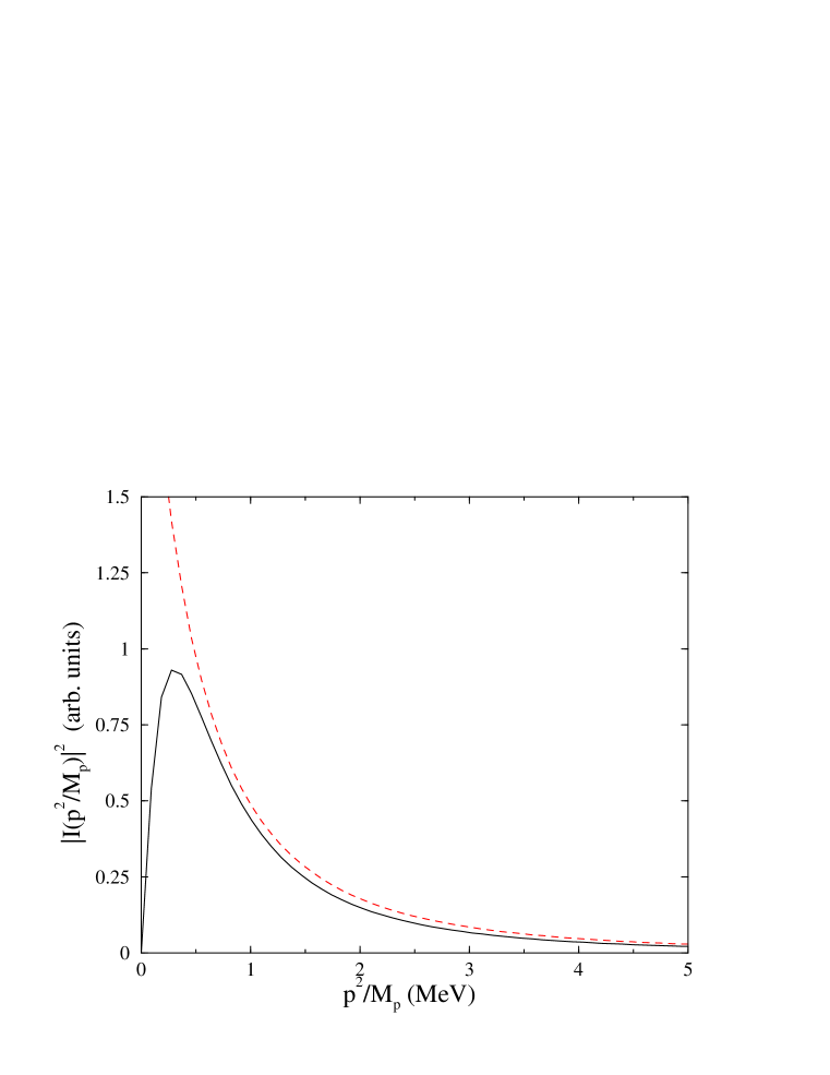
FIG. 1.: Radial integral $|I(p^{2}/M_{p})|^{2}$. Exact result (solid line) and scaled approximation with Coulomb repulsion and effective range set to zero (dashed line) are shown.

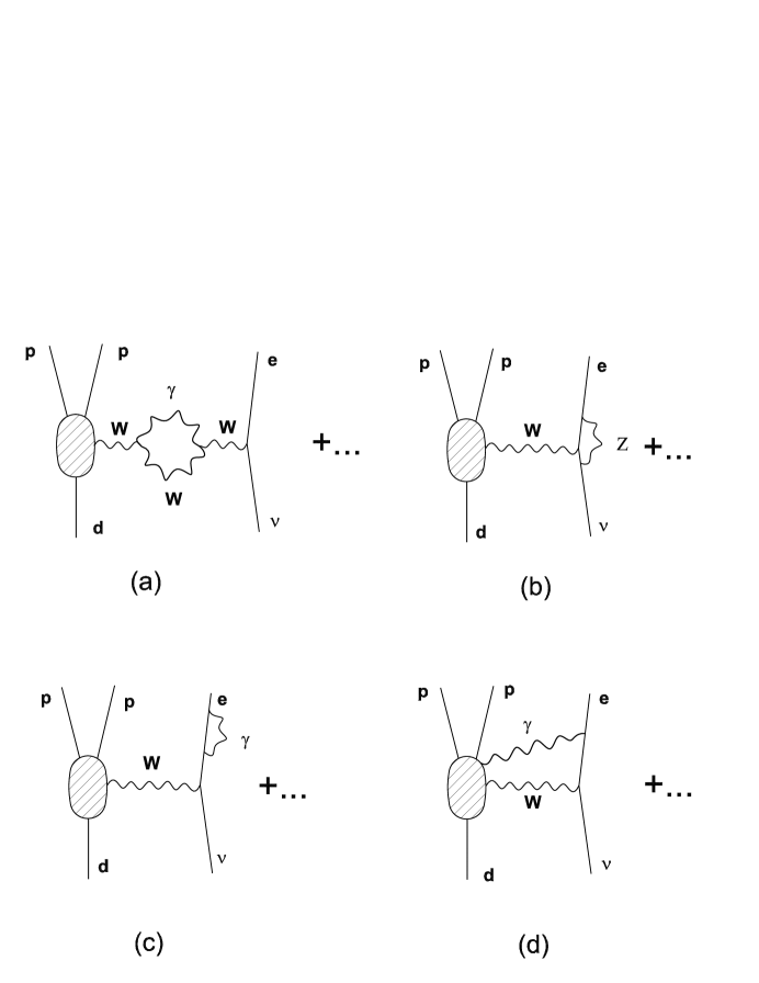
FIG. 2.: Order $\alpha$ radiative corrections to the charged-current breakup of deuteron: $d+\nu_{e}\rightarrow p+p+e$ involving virtual $\gamma$ quanta and $Z$ boson exchange. The large shaded oval represents the vertex with all its hadronic complications.

FIG. 3.: Order $\alpha$ corrections due to bremsstrahlung emission. See caption to Fig. 2.

FIG. 4.: Corrections to the differential cross-sections as a function of the observed energy, normalized to the total tree-level cross-section. Solid line corresponds to $E_{\gamma}^{min}\rightarrow\infty$ ($E_{obs}=E_{e}$), dashed line to $E_{\gamma}^{min}\rightarrow 0$ ($E_{obs}=E_{e}+E_{\gamma}$), and the dot-dashed line is obtained by setting $E_{obs}=E_{e}+(E_{\gamma}-1)\theta(E_{\gamma}-1)$. All lines are evaluated for $E_{\nu}$ = 10 MeV.

FIG. 5.: Correction to the cross section for $E_{\gamma}^{min}\rightarrow 0$. Note that in this case the corrections does not depend on $E_{\nu}$.

FIG. 6.: Radiative corrections to the CC total cross section as a function of neutrino energy.

FIG. 7.: Radiative corrections to the total CC cross section folded with the incoming ⁸B $\nu_{e}$ spectrum as a function of the detected energy $E_{obs}$ (full line) Also shown is similarly folded tree level CC reaction cross section, scaled by a factor of 1/40 (dashed line).

FIG. 8.: Feynman graphs relevant for the radiative correction to the NC cross section (see text for explanation).

REFERENCES

- [1] Q. R. Ahmad et al. Phys. Rev. Lett. 87, 071301 (2001).
- [2] S. Fukuda et al. Phys. Rev. Lett. 86, 5651 (2001).
- [3] J. N. Bahcall, M. H. Pinsonneault, and J. P. Zahn, Astrophys. J. 555, 990 (2001).
- [4] A. S. Brun, S. Turck-Chièze, and J. P. Zahn, Astrophys. J. 525, 1032 (1999); S. Turck-Chièze et al. Astrophys. J. Lett. 555, L69 (2001).
- [5] S. Nakamura, T. Sato, V. Gudkov, and K. Kubodera, Phys. Rev. C 63, 034617 (2001); M. Butler, J.-W.Chen, and X. Kong, Phys. Rev. C 63, 035501 (2001).
- [6] I. S. Towner, Phys. Rev. C 58, 1288 (1998).
- [7] J. F. Beacom and S. J. Parke, Phys. Rev. D 64, 091302 (2001); hep-ph/0106128.
- [8] A. Sirlin, Rev. Mod. Phys. 50, 573 (1978).
- [9] R. G. H. Robertson, private communication.
- [10] F. J. Kelly and H. Überall, Phys. Rev. Lett. 16, 145 (1966).
- [11] S. D. Ellis and J. N. Bahcall, Nucl. Phys. A114, 636 (1968).
- [12] X. Ji and M.J. Musolf, Phys. Lett. B257, 409 (1991).
- [13] Particle Data Group, Review of Particle Properties, E. Phys. J. C 15, 1 (2000). See, in particular, Table 10.3.
- [14] I.S. Towner and J.C. Hardy, in Symmetries and Fundamental Interactions in Nuclei, W.C. Haxton and E.M. Henley, eds., World Scientific (Singapore) 1995, p.183-250.
- [15] P. Vogel, Phys. Rev. D 29, 1918 (1984).
- [16] S. A. Fayans, Sov. J. Nucl. Phys. 42, 590 (1985).
- [17] J. N. Bahcall and B. R. Holstein, Phys. Rev. C 33, 2121 (1986).
- [18] M.J. Musolf, et al., Phys. Rep. 239, 1 (1994).
- [19] I. S. Batkin and M. K. Sundaresan, Phys. Rev. D 52, 5362 (1995).
- [20] J. C. Hardy and I. S. Towner, nucl-th/9812036.