Three- and Four-body correlations in nuclear matter

Abstract

Few-nucleon correlations in nuclear matter at finite densities and temperatures are explored. Using the Dyson equation approach leads to effective few-body equations that include self energy corrections and Pauli blocking factors in a systematic way. Examples given are the nucleon deuteron in-medium reaction rates, few-body bound states including the $\alpha$-particle, and $\alpha$-particle condensation.

1 Introduction

Strongly correlated many-particle systems provide an exciting field for applications of few-body methods. Examples are nuclear matter, quark matter (quark gluon plasma), ionic plasmas, among others. In an equilibrium situation at finite temperatures and densities one usually introduces a mean field to describe the gross features of many-particle systems. However, many exciting phenomena, such as the formation of clusters below a certain density (Mott density) and the appearance of superconductivity below a critical temperature, cannot be described in a framework of noninteracting quasiparticles (ideal system). Within a quantum statistical approach it is possible to go beyond such a picture and consider the residual interactions between the quasiparticles. A well known equation, e.g., to study two-body correlations is known as Bethe-Goldstone equation and/or Feynman-Galitskii equation, depending on details [1]. To go beyond two-body correlations is desirable for many reasons. Among them are: i) For a microscopic description of the heavy ion collision, three-body reaction rates are an important input into the collision integral. Their medium dependence has hardly been studied [2, 3, 4, 5]. ii) Bound states are effected by the density and temperature of the medium and the binding energy may become zero leading to the Mott effect [6, 7, 8, 9, 10]. iii) Since the $\alpha$-particle is the strongest bound nucleus it should be relevant for the equation of state of nuclear matter. It might induce $\alpha$-condensation and quartetting which would be a different state of matter besides superfluidity induced by pairing or pair condensation [11]. iv) The three-quark system is particularly interesting because it is a reasonable model of baryons and useful to study the phase transition between the quark phase and the hadronic phase of nuclear matter [12, 13]. v) The three-body input into the two-body t-matrix implied by the equations hierarchy has not been studied and might, e.g., affect the critical temperature.

The first three issues will be addressed in the following, iv) is given to some detail in Ref. [13] of this issue, and v) is left for future investigations and is relevant, e.g., for the question of a possible color superconducting phase.

2 Theoretical tools

We utilize the Dyson equations to tackle the many-particle problem. An review is given in Ref. [14]. This enables us to decouple the hierarchy of equations finally deriving effective in-medium few-body equations. The many-particle Hamiltonian is given by

$$H=\sum_{1}H_{0}(1)a_{1}^{\dagger}a_{1}+\;\frac{1}{2}\;\sum_{121^{\prime}2^{\prime}}V_{2}(12,1^{\prime}2^{\prime})\;a^{\dagger}_{1}a^{\dagger}_{2}a_{2^{\prime}}a_{1^{\prime}}$$ (1)

where $H_{0}$ is the single particle energy and $V_{2}$ a generic two-body potential. The chronological equal time cluster Green function for a given number of particles is defined by

$${\cal G}_{\alpha\beta}^{\tau-\tau^{\prime}} = -i\langle T_{\tau}A_{\alpha}(\tau)A_{\beta}^{\dagger}(\tau^{\prime})\rangle,\qquad{\langle\dots\rangle={\rm Tr}\{\rho_{0}\dots\}}$$ (2)

where $A_{\alpha}=a_{1}a_{2}a_{3}\dots a_{n}$, e.g., are Heisenberg operators and $\rho_{0}$ the equilibrium density operator. The respective Dyson equation for the cluster is

$$i\frac{\partial}{\partial\tau}\;{\cal G}^{\tau-\tau^{\prime}}_{\alpha\beta} = \delta(\tau-\tau^{\prime})\underbrace{\langle[A_{\alpha},A_{\beta}^{\dagger}]_{\pm}\rangle}_{=:{\cal N}^{\tau}_{\alpha\beta}}+\sum_{\gamma}\int d\bar{\tau}\;{{\cal M}^{\tau-\bar{\tau}}_{\alpha\gamma}}\;{\cal G}^{\bar{\tau}-\tau^{\prime}}_{\gamma\beta}.$$ (3)

The mass matrix that appears in (3) is given by

$${\cal M}^{\tau-\tau^{\prime}}_{\alpha\beta} = \underbrace{\delta(\tau-\tau^{\prime}){\cal M}^{\tau}_{\alpha\beta,0}}_{\mbox{\rm cluster mean field}}+\underbrace{{\cal M}^{\tau-\tau^{\prime}}_{\alpha\beta,\rm irr.}}_{\mbox{\rm retardation}}$$ (4)

$$({\cal M}{\cal N})^{\tau}_{\alpha\beta,0} = \langle[[A_{\alpha},H](\tau),A_{\beta}^{\dagger}(\tau)]\rangle$$ (5)

$$({\cal MN})^{\tau-\tau^{\prime}}_{{\rm irr.},\alpha\beta} = \sum_{\gamma}\langle T_{\tau}[A_{\alpha},H]_{\tau},[A^{\dagger}_{\beta},H]_{\tau^{\prime}}]\rangle_{{\rm irreducible}}.$$ (6)

More details are given in [14]. The equation (3) is expressed in momentum space and the time component as Matsubara frequency $\tau\rightarrow z_{\lambda}$ that is analytically continued into the complex plane, $z_{\lambda}\rightarrow z$, for a textbook treatment see [1]. To arrive at suitable calculable expressions the following approximations are utilized: i) Only the cluster mean field contribution to the kernel (4) is used; ii) The density operator $\rho$ is evaluated for an uncorrelated medium. This way the equations hierarchy is decoupled and effective few-body equations that describe few-body correlations including medium effects have been derived. For $A_{\alpha}=a_{1}$, the one-particle Green functions is

$$G(z)=(z-\varepsilon_{1})^{-1}$$ (7)

where the quasi-particle self energy is

$$\varepsilon_{1}=\frac{k^{2}_{1}}{2m_{1}}+\sum_{2}V_{2}(12,\widetilde{12})f_{2}\simeq\frac{k^{2}_{1}}{2m_{1}^{\rm eff}}+\Sigma^{\rm HF}(0).$$ (8)

The last equation introduces the effective mass that is a valid concept for the rather low densities considered here and $\mu^{\rm eff}\equiv\mu-\Sigma^{\rm HF}(0)$. The Fermi function $f_{i}\equiv f(\varepsilon_{i})$ for the $i$-th particle is given by

$$f(\varepsilon_{i})=\frac{1}{e^{\beta(\varepsilon_{i}-\mu)}+1}.$$ (9)

The resolvent $G_{0}$ for $n$ noninteracting quasiparticles is

$$G_{0}(z)=(z-H_{0})^{-1}N\equiv R_{0}(z)N,\qquad H_{0}=\sum_{i=1}^{n}\varepsilon_{i}$$ (10)

where $G_{0}$, $H_{0}$, and $N$ are formally matrices in $n$ particle space. The Pauli-blocking for $n$-particles is

$$N=\bar{f}_{1}\bar{f}_{2}\dots\bar{f}_{n}\pm f_{1}f_{2}\dots f_{n},\qquad\bar{f}=1-f$$ (11)

where the upper sign is for Fermi-type and the lower for Bose type clusters. Note that $NR_{0}=R_{0}N$. Straight forward evaluation of (3) using the Wick theorem leads also to the full resolvent $G(z)$. For each number of particles in the cluster the resolvents have the same formal structure and can be written in a convenient way close to the one for the isolated system, viz.

$$G(z)=(z-H_{0}-V)^{-1}{N}\equiv R(z){N},\qquad V\equiv\sum_{\mathrm{pairs}\;\alpha}N_{2}^{\alpha}V_{2}^{\alpha}.$$ (12)

Note that $V^{\dagger}\neq V$ and $R(z)N\neq NR(z)$. To be specific, for an interaction in pair $\alpha=(12)$ the effective potential reads

$$\langle 123\dots|{N_{2}^{(12)}}V_{2}^{(12)}|1^{\prime}2^{\prime}3^{\prime}\dots\rangle={(\bar{f}_{1}\bar{f}_{2}-f_{1}f_{2})}V_{2}(12,1^{\prime}2^{\prime})\delta_{33^{\prime}}\dots$$ (13)

For further use in the Alt Grassberger Sandhas (AGS) equations [15] we give also the channel resolvent

$$G_{\alpha}(z)=(z-H_{0}-N_{2}^{\alpha}V_{2}^{\alpha})^{-1}N\equiv R_{\alpha}(z)N.$$ (14)

For the two-body case as well as for a two-body subsystem embedded in the $n$-body cluster the standard definition of the $t$ matrix leads to the Feynman-Galitskii equation for finite temperature and densities [1],

$$T_{2}^{\alpha}(z)=V_{2}^{\alpha}+V_{2}^{\alpha}N^{\alpha}_{2}R_{0}(z)T_{2}^{\alpha}(z).$$ (15)

Introducing the AGS transition operator via

$$R(z)=\delta_{\alpha\beta}R_{\alpha}(z)+R_{\alpha}(z){U_{\alpha\beta}(z)}R_{\beta}(z)$$ (16)

the effective inhomogeneous in-medium AGS equation reads

$$U_{\alpha\beta}(z)=(1-{\delta}_{\alpha\beta})R^{-1}_{0}(z)+\sum_{\gamma\neq\alpha}{N^{\gamma}_{2}}T_{2}^{\gamma}(z)R_{0}(z)U_{\gamma\beta}(z).$$ (17)

The homogeneous in-medium AGS equation uses the form factors defined by

$$|F_{\beta}\rangle\equiv\sum_{\gamma}\bar{\delta}_{\beta\gamma}{N_{2}^{\gamma}}V_{2}^{\gamma}|\psi_{B_{3}}\rangle$$ (18)

to calculate the bound state $\psi_{B_{3}}$. Because of the non-symmetric form of the potential the equation for the form factors and the dual are different

$$|F_{\alpha}\rangle = \sum_{\beta}\bar{\delta}_{\alpha\beta}{N_{2}^{\beta}}T_{2}^{\beta}(B_{3})R_{0}(B_{3})|F_{\beta}\rangle$$ (19)

$$|\tilde{F}_{\alpha}\rangle = \sum_{\beta}\bar{\delta}_{\alpha\beta}T_{2}^{\beta}(B_{3}){N_{2}^{\beta}}R_{0}(B_{3})|\tilde{F}_{\beta}\rangle.$$ (20)

Finally, the four-body bound state is described by

$$|{\cal F}^{\sigma}_{\beta}\rangle=\sum_{\tau\gamma}\bar{\delta}_{\sigma\tau}\underbrace{U^{\tau}_{\beta\gamma}(B_{4})}_{\mbox{3-body}}R_{0}(B_{4}){N_{2}^{\gamma}}\underbrace{T_{2}^{\gamma}(B_{4})}_{\mbox{2-body}}R_{0}(B_{4})|{\cal F}^{\tau}_{\gamma}\rangle,\qquad\alpha\subset\sigma,\gamma\subset\tau.$$ (21)

where $\sigma,\tau$ denote the four-body partitions. The two-body input is given in (15) and the three-body input by (17), both medium dependent.

3 Results

3.1 Reaction rates

An experiment to explore the equation of state of nuclear matter is heavy ion collisions at various energies. Here we focus on intermediate to low scattering energies and compare results to a recent experiment ¹²⁹Xe+¹¹⁹Sn at 50 MeV/A by the INDRA collaboration [16]. A microscopic approach to tackle the heavy ion collision is given by the Boltzmann equation for different particle distributions $F\equiv(f_{p},f_{n},f_{d},f_{t},f_{h})$ up to $h$ and $t$ [9, 10],

$$\frac{\partial}{\partial t}F(t)+\{\varepsilon,F(t)\}={\cal K}^{\rm in}_{i}[F(t)]\,(F(t)\pm 1)-{\cal K}^{\rm out}_{i}[F(t)]\,F(t)$$ (22)

where $\varepsilon$ is the mean field energy and ${\cal K}$ denotes the respective collision integrals that include, e.g., the one for deuteron loss $Nd\rightarrow NNN$,

$${\cal K}^{\rm out}_{d}(P,t) = \int d^{3}k\int d^{3}k_{1}d^{3}k_{2}d^{3}k_{3}\;\underbrace{|\langle k_{1}k_{2}k_{3}|U_{0}|kP\rangle|^{2}_{dN\rightarrow pnN}}_{\mbox{medium dependent!}}$$ (23)

$$\qquad\times\bar{f}_{N}(k_{1},t)\bar{f}_{N}(k_{2},t)\bar{f}_{N}(k_{3},t)f_{N}(k,t)+\dots$$

where $\bar{f}\equiv 1-f$. A solution is given via a Boltzmann Uehling Uhlenbeck (BUU) simulation  [9, 10]. As indicated in (23) the reaction rate is in principle medium dependent. However, previously this medium dependence has been neglected. Within linear response theory for infinite nuclear matter the use of in-medium rates leads to faster time scales for the deuteron life time and the chemical relaxation time as has been shown in detail in Refs. [3, 4].

Figure 1: BUU simulation of the deuteron formation during the central collision of ¹²⁹Xe+¹¹⁹Sn at 50 MeV/A.

Figure 2: Ratio of proton to deuteron numbers as a function of c.m. energy. The experimental data are from the INDRA collaboration.

Now we use the in-medium AGS equations (17) that reproduce the experimental data in the limit of an isolated three-body system. For details on the specific interaction model see Ref. [2]. We investigate the influence of medium dependent rates in the BUU simulation of the heavy ion collision as compared to use of isolated (i.e. experimental) rates. Figure 2 shows that the net effect (gain-minus-loss, eq.(23)) of deuteron production becomes larger for the use of in-medium rates (solid line) compared to using the isolated rates (dashed line). The change is significant, however, a comparison with experimental data is difficult since deuterons may also be evaporating from larger clusters that has not been taken into account in the present calculation so far. The ratio of protons to deuterons may be better suited for a comparison to experiments that is shown in Figure 2. The use of in-medium rates (solid line) lead to a shape closer to the experimental data (dots) than the use of isolated rates (dashed line).

3.2 Bound states, Mott effect

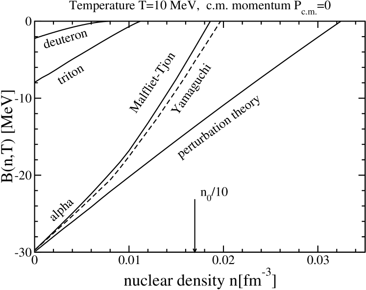
Figure 3: Difference between the pole energy of the bound state and the continuum, $B(n,T)=E_{\rm pole}-E_{\rm cont}$.

Figure 4: Critical temperatures of condensation/pairing leading to superfluid nuclear matter. For an explanation see text.

In these calculation, besides the change of rates, also the Mott effect has been taken into account. Figure 4 shows the dependence of the binding energy for different clusters at a given temperature of $T=10$ MeV and at rest in the medium. At first sight an Efimov effect [17] might be expected in the vicinity of the Mott transition of the deuteron. However, two main reasons prevent the Efimov effect to appear in a simple way: i) The deuteron binding energy in the medium depends parametric (through the blocking factors) on the deuteron momentum. Since the deuteron-like subsystem is not at rest, in other words the effective strength of the potential that enters into the three-body problem varies with momenta, a possible Efimov effect is washed out. ii) The excited states that should appear from the continuum (Efimov states) are as well blocked by the medium. This blocking may not be so strong as the ground states, because the momentum distribution is peaked at higher momenta. As a consequence only a careful quantitative analysis might answer the question of Efimov states. On the other hand nuclear matter might not be the best system to eventually observe such an effect.

In Figure 4 part of the phase diagram of nuclear matter is shown. The lines indicate phase transitions. The critical temperatures of condensation/pairing (dashed line, [11]) leading to superfluid nuclear matter are shown. The possible area of $\alpha$ condensation (solid line) as suggested by [11] is also given. The latter is based on a variational calculation using the 2+2 component of the $\alpha$ particle to evaluate the condition for the onset of superfluidity for the four-particle system $B(T_{c},\mu,P=0)=4\mu$. The critical temperature found by solving the homogeneous AGS equation for $\mu<0$ confirms the onset of $\alpha$ condensation even at higher values (dotted line). For $\mu>0$ the condition $B=4\mu$ for the phase transition can also be fulfilled. However, the homogeneous AGS equation cannot be used to investigate the steep fall-off predicted in Ref. [11] because of continuum poles that are not compensated by the blocking factors of the potential as is the case for the two-body problem. Whether the steep fall-off is of physical origin or due to the use of a homogeneous equation also for $\mu>0$ needs further investigation.

Work supported by Deutsche Forschungsgemeinschaft.

References

- [1] Kadanoff L. P., Baym G.: Quantum statistical mechanics (Benjamin, New York 1962); Fetter A. L., Walecka J.D.: Quantum Theory of Many-Particle Systems, (McGraw-Hill, New York 1971)
- [2] Beyer M., Röpke G. and Sedrakian A.: Phys. Lett. B376, 7 (1996)
- [3] Beyer M. and Röpke G.: Phys. Rev. C 56, 2636 (1997)
- [4] Kuhrts C., Beyer M. and Röpke G.: Nucl. Phys. A668, 137 (2000)
- [5] Kuhrts C., Beyer M., Danielewicz P.D. and Röpke G.: Phys. Rev. C 63, 034605 (2001)
- [6] Beyer M., Schadow W., Kuhrts C. and Röpke G.: Phys. Rev. C 60, 034004 (1999)
- [7] Beyer M.: Few Body Systems Suppl. 10, 179 (1999)
- [8] Beyer M., Sofianos S.A., Kuhrts C., Röpke G. and Schuck P.: Phys. Lett. B488, 247 (2000)
- [9] Danielewicz P. and Bertsch G.F.: Nucl. Phys. A 533, 712 (1991)
- [10] Danielewicz P. and Pan Q.: Phys. Rev. C 46, 2002 (1992)
- [11] Röpke G., Schnell A., Schuck P., Nozieres P.: Phys. Rev. Lett. 80, 3177 (1998)
- [12] Beyer M., Mattiello S., Frederico T. and Weber H.J.: Phys. Lett. B (2001) in print [arXiv:hep-th/0106219].
- [13] Mattiello S., Beyer M., Frederico T. and Weber H.J.: Few-Body Systems, this issue.
- [14] Dukelsky J., Röpke G. and Schuck P.: Nucl. Phys. A 628, 17 (1998)
- [15] Alt E. O., Grassberger P. and Sandhas W.: Nucl. Phys. B 2, 167 (1967 )
- [16] INDRA collaboration, Gorio D. et al.: Eur. Phys. J. A 7 245 (2000) and ref. therein
- [17] Efimov V.N.: Phys. Lett. 33B, 563 (1970), Sov. J. Nucl. Phys. 12, 589 (1971)