The Hypertriton in Effective Field Theory

Abstract

Doublet $\Lambda d$ scattering and the hypertriton are studied in the framework of an effective field theory for large scattering lengths. As in the triton case, consistent renormalization requires a one-parameter three-body force at leading order whose renormalization group evolution is governed by a limit cycle. Constraining unknown parameters from symmetry considerations and the measured binding energy of the hypertriton, we calculate the low-energy phase shifts for doublet $\Lambda d$ scattering. For the low-energy parameters, we find $a_{\Lambda d}=(16.8^{+4.4}_{-2.4})$ fm and $r_{\Lambda d}=(2.3\pm 0.3)$ fm, where the errors are due to the uncertainty in the hypertriton binding energy. Since the hypertriton is extremely shallow, low-energy three-body observables in this channel are very insensitive to the exact values of the $\Lambda N$ low-energy parameters.

I Introduction

In recent years, there has been much interest in applying Effective Field Theory (EFT) methods to nuclear systems with two or more nucleons Weinberg ; NN98 ; NN99 ; Birareview ; Bea00 . EFT’s provide a powerful framework to explore a separation of scales in physical systems in order to perform systematic, model-independent calculations EFT . If, for example, the momenta $k$ of two particles are much smaller than the inverse range of their interaction $1/R$, observables can be expanded in powers of $kR$. All short-distance effects are systematically absorbed into a few low-energy constants using renormalization. The EFT approach allows for accurate calculation of low-energy processes with well-defined error estimates. For low-energy nuclear few-body systems, the long-distance scale is set by the large two-body scattering lengths, while the short distance scale is set by the range of the nuclear force or the inverse pion mass. In an EFT, the long-distance physics is included explicitly, while the corrections from short-distance physics are calculated in an expansion in the ratio of these two scales.

For very low energies and momenta ($p\hskip 1.99997pt\raisebox{2.15277pt}{$<$}\raisebox{-3.00003pt}{$\sim$}\hskip 1.99997ptm_{\pi}$), even pion exchange can be considered “short-distance” physics. In this case, one can use an effective Lagrangian including only contact interactions. The large S-wave scattering lengths require that the leading two-body contact interaction is treated nonperturbatively vKo99 ; KSW98 . In the two-body system, this program has been very successful (see e.g. Refs. Bea00 ; CRS99 ; BeS00 and references therein).

In the nuclear three-body system, considerable progress has been made as well BeK98 ; BHK98 ; BHK99 ; BeG00 ; GBG00 ; RuK01 ; BHK00 ; BlG00 ; HaM01 ; HaM01b . Most of the work has concentrated on the neutron-deuteron system. In channels where the Pauli principle or centrifugal barrier suppress sensitivity to short-distance physics, the EFT can be extended in a straightforward way BeK98 ; BHK98 ; BeG00 ; GBG00 . Recently, Coulomb repulsion has been included and the phase shifts for proton-deuteron scattering in the spin quartet ($J=3/2$) have been calculated RuK01 . Most interesting, however, is the S-wave in doublet ($J=1/2$) neutron-deuteron scattering which displays a number of surprising phenomena such as the Thomas and Efimov effects or the Phillips line Tho35 ; Phi68 ; Efi71 . In this channel, the renormalization requires a one-parameter three-body force at leading order whose renormalization group evolution is governed by a limit cycle BHK99 ; BHK00 . Variation of this three-body force gives a compelling explanation of the Phillips line Phi68 . Recently, the effective range corrections to S-wave neutron-deuteron scattering in the doublet channel have been calculated HaM01b . At this order, good agreement with available phase shift analyses and potential model calculations is obtained.

The purpose of the present paper is to study doublet $\Lambda d$ scattering and the hypertriton using EFT methods. The hypertriton is the lightest hypernucleus and consists of a triton with one neutron replaced by a $\Lambda$. It is the simplest strange three-body halo nucleus with a separation energy into a deuteron and a $\Lambda$ of only $B^{\Lambda}=0.13\pm 0.05$ MeV Jur73 ; Dav91 . The total binding energy is $B_{3}^{\Lambda}=2.35$ MeV. The hypertriton has been studied extensively using various hyperon-nucleon potentials (see e.g. Refs. ClL85 ; AfG89 ; Con92 ; MiG93 ; CJF97 ; FeJ01 and references therein). The most sophisticated calculations include both tensor forces and $\Lambda\leftrightarrow\Sigma$ conversion effects AfG89 . Obtaining the correct binding energy for the hypertriton in these potential models is delicate, which has motivated the use of this system to study details of the hyperon-nucleon interaction CJF97 .

The EFT framework offers a different perspective and stresses the universal aspects of the problem. In this paper, we study $\Lambda d$ scattering and the hypertriton in the framework of an EFT for three-body systems with large two-body scattering lengths BHK99 ; BHK00 . The small $N-\Lambda$ mass difference can be exploited by expanding in the parameter $y=(M_{\Lambda}-M)/(M_{\Lambda}+M)\approx 0.1$. After this expansion is performed, the hypertriton emerges naturally as a shallow Efimov state. To leading order, both $NN$ and $\Lambda N$ S-waves will contribute to the hypertriton. While the $NN$ S-waves have a large scattering length, the $\Lambda N$ scattering lengths are believed to be natural. Therefore, it is not obvious that an EFT for large two-body scattering lengths is applicable. In the following, we motivate the use of this EFT.

Unfortunately, there are only few $\Lambda N$ scattering data and these are at relatively high energies. Model independent analyses using effective range theory indicate mainly S-wave scattering, but afford many solutions for the low-energy parameters and are essentially inconclusive Ale68 ; Sec68 . For example in Ref. Sec68 , the extracted one-standard-deviation bounds were $0>a_{1}>-15$ fm, $0<r_{1}<15$ fm, $-0.6$ fm $>a_{3}>-3.2$ fm, and $2.5$ fm $<r_{3}<15$ fm where $a_{1}$ ($a_{3}$) and $r_{1}$ ($r_{3}$) are the singlet (triplet) scattering length and effective range, respectively. These bounds do not exclude the case of large scattering lengths.

Various sets of low-energy parameters are also known from extrapolations of the few higher energy data using hyperon-nucleon potentials NRS73 ; RSY99 ; CJF97 ; HHS89 ; RHS94 . The extracted $\Lambda N$ scattering lengths and effective ranges are generally of natural size [${\cal O}(1/m_{\pi})$]. Both the ${}^{3}S_{1}$ and ${}^{1}S_{0}$ $\Lambda N$ partial waves have a virtual bound state. The pole momenta extracted from the low-energy extrapolations are $\sim 60$ MeV for the ${}^{1}S_{0}$ and $\sim 70$ MeV for the ${}^{3}S_{1}$ partial wave. However, it is not clear how large the errors and model-dependence in these low-energy extrapolations are.

An EFT analysis of hyperon nucleon scattering and hyperon mass shifts in the nuclear medium was recently performed in Ref. KDT01 . The $\Lambda N$ scattering lengths, however, were used as input in this analysis.

Because the hypertriton is so weakly bound, it should only be sensitive to the extreme long-distance properties of the $\Lambda N$ interaction. The typical momentum scale of the hypertriton can be estimated from its binding energy via

$$\gamma_{3}^{\Lambda}\sim 2\sqrt{(MB_{3}^{\Lambda}-\gamma_{d}^{2})/3}\approx 0.3\gamma_{d}\,,$$ (1)

where $M=938.9$ MeV is the nucleon mass and $\gamma_{d}=45.68$ MeV the deuteron pole momentum. Since $\gamma_{3}^{\Lambda}$ is so small, the contribution from the effective ranges will be suppressed even if the $\Lambda N$ low-energy parameters are ${\cal O}(1/m_{\pi})$ as extracted from the potential models (see Section IV for a more quantitative estimate). Consequently, the use of the EFT for large two-body scattering lengths is justified.

In the next Section, we write down the effective Lagrangian and discuss the power counting of the EFT. We then review the EFT for the $NN$ and $\Lambda N$ two-body subsystems. In Section III, we obtain the three-body integral equations for the $\Lambda NN$ system and in Section IV we present our results and conclusions. Some technical details are given in the Appendices.

II Two-Body System

The power counting in an EFT is determined by the physical scales in the system under consideration. For the hypertriton, we are only interested in very low-energies, where all physics (even pion exchange) can be considered “short-range”. The two-body subsystems ($NN$ and $\Lambda N$) are characterized by two scales: a long-distance scale (the large S-wave scattering length) and a short-distance scale that is given by the longest-range physics excluded from the EFT. For an EFT without pions, one expects the short-distance scale $R$ to be of ${\cal O}(1/m_{\pi})$. However, since the $\Lambda\;(I=0)$ and nucleon ($I=1/2$) cannot exchange a pion with $I=1$ and conserve isospin, the short-distance scale for the hypertriton should be set by the two-pion exchange AfG89 . A power counting to deal with unnaturally large two-body scattering lengths has been proposed in Refs. vKo99 ; KSW98 . This counting takes $p\sim 1/a\sim Q$, where $p$ is the typical momentum and $1/a$ is the inverse scattering length. The pole or binding momentum $\gamma$ is of ${\cal O}(Q)$ as well since $\gamma=1/a+{\cal O}(r/a^{2})$ with $r\sim R$ the effective range. The expansion of the EFT is in powers of $QR\approx\gamma r$ (see Refs. GBG00 ; HaM01b for more details).

For the study of three-body systems, it is convenient to employ the dibaryon formalism Kap97 , where an auxiliary field is used to describe two baryons interacting in a given partial wave. We write down an effective Lagrangian including nucleons, $\Lambda$’s, and dibaryon fields for the deuteron ($d$) as well as the ${}^{3}S_{1}$ ($u^{3}$) and ${}^{1}S_{0}$ ($u^{1}$) $\Lambda N$ partial waves,

$${\cal L} = N^{\dagger}\left(i\partial_{t}+\frac{\vec{\nabla}^{2}}{2M}\right)N+\Lambda^{\dagger}\left(i\partial_{t}+\frac{\vec{\nabla}^{2}}{2M_{\Lambda}}\right)\Lambda$$

$$+\Delta_{d}d_{l}^{\dagger}d_{l}-\frac{g_{d}}{2}\left[d_{l}^{\dagger}N^{T}(i\tau_{2})(i\sigma_{l}\sigma_{2})N+\mbox{H.c.}\right]$$

$$+\Delta_{3}(u^{3}_{l})^{\dagger}u^{3}_{l}-ig_{3}\left[(u^{3}_{l})^{\dagger}\Lambda^{T}(i\sigma_{l}\sigma_{2})N+\mbox{H.c.}\right]$$

$$+\Delta_{1}(u^{1})^{\dagger}u^{1}-ig_{1}\left[(u^{1})^{\dagger}\Lambda^{T}(i\sigma_{2})N+\mbox{H.c.}\right]+\ldots\,,$$

where H.c. denotes the Hermitian conjugate and the dots indicate terms with more derivatives and/or fields. The terms with more derivatives are suppressed at low energies, while four- and higher-body forces do not contribute. Three-body terms will be addressed in the next Section. In Eq. (II), indices occuring repeatedly are summed over and $\sigma_{i}$ ($\tau_{i}$) are the usual Pauli matrices acting in spin (isospin) space. Spinor and isospinor indices are suppressed. The parameters $\Delta$ and $g$ are not independent and only the combination $\Delta/g^{2}$ enters physical observables.

The Lagrangian (II) describes low-energy S-wave scattering of nucleons and $\Lambda$’s and reproduces the effective range expansion up to the scattering length term, which is sufficient for our purposes. To go to higher orders in $QR$, the two-body effective range can be included with a kinetic term for the auxiliary field Kap97 . Only the partial waves contributing in the hypertriton channel to leading order in $QR$ are included in the effective Lagrangian (II). The ${}^{1}S_{0}$ $NN$ amplitude does not contribute because of isospin, while higher partial waves and the tensor force are suppressed by at least two powers of the expansion parameter $QR$ GBG00 . After integrating out the auxiliary fields $d$, $u^{3}$, and $u^{1}$, it is straightforward to show that the Lagrangian (II) is equivalent to a Lagrangian with nucleon and $\Lambda$ fields only (cf. Refs. BHK99 ; BHK00 ).

Since the theory is nonrelativistic, all particles propagate forward in time and the nucleon and $\Lambda$ tadpoles vanish. The propagator for nucleons and $\Lambda$’s is simply

$$iS(p_{0},\vec{p})=\frac{i}{p_{0}-\vec{p}^{\,2}/(2m)+i\epsilon}\,,$$ (3)

where $m$ is the mass of the corresponding particle. The dibaryon propagators are more complicated because of the coupling to two-baryon states. The bare dibaryon propagators are constant, $i/\Delta$, but the full propagators are dressed by baryon loops to all orders, as illustrated for the $\Lambda N$ state in Fig. 1.

Figure 1: Dressing of the bare $\Lambda N$ propagator. The dashed line indicates a $\Lambda$, the solid line a nucleon, the thick solid line a bare, and the double line a full dibaryon propagator.

All diagrams in Fig. 1 are of the same order because $2\pi\Delta/(Mg^{2})=1/a\sim Q$. Summing the resulting geometric series leads to

$$iD_{j}(p_{0},\vec{p})=\frac{2\pi}{\mu_{\Lambda}g_{j}^{2}}\frac{-i}{-\gamma_{j}+\sqrt{-2\mu_{\Lambda}\left(p_{0}-\vec{p}^{\,2}/\left[2(M+M_{\Lambda})\right]\right)-i\epsilon}}\,,$$ (4)

where $\mu_{\Lambda}=MM_{\Lambda}/(M+M_{\Lambda})$ is the reduced mass of the $\Lambda N$ system, $j\in\{1,3\}$, and $\gamma_{j}$ is the corresponding pole momentum. Divergent loop integrals are regulated using dimensional regularization. The full propagator for the deuteron is BHK98 ; BHK00

$$iD_{d}(p_{0},\vec{p})=\frac{2\pi}{Mg_{d}^{2}}\frac{-i}{-\gamma_{d}+\sqrt{-Mp_{0}+\vec{p}^{\,2}/4-i\epsilon}}\,,$$ (5)

where $\gamma_{d}=45.68$ MeV is the deuteron pole momentum. The values of $\gamma_{1}$ and $\gamma_{3}$ will be discussed later, together with the three-body results. The scattering amplitudes are obtained by attaching external baryon lines to the full propagators from Eqs. (4,5) BHK00 . All dependence on the bare coupling constants $g_{d}$, $g_{1}$, and $g_{3}$ cancels in observable quantities.

III Three-Body System

We now apply the Lagrangian (II) to the $\Lambda NN$ system in the $J=1/2$ channel, which has the hypertriton as a three-body bound state. We do not include explicit $\Lambda\leftrightarrow\Sigma$ conversion effects AfG89 . Such effects are accounted for by a $\Lambda NN$ three-body force to be introduced in the following. Explicit $\Sigma$ degrees of freedom have been integrated out from the effective Lagrangian. This procedure is justified because the characteristic momentum $\gamma_{3}^{\Lambda}\ll\sqrt{M_{\Lambda}(M_{\Sigma}-M_{\Lambda})}\approx 300$ MeV Sav97 .

To leading order in $QR$, only relative S-waves contribute. A $\Lambda NN$ state with the quantum numbers of the hypertriton ($J^{P}=\frac{1}{2}^{+}$) can then be constructed in three different ways: $(i)$ a ${}^{3}S_{1}$ $\Lambda N$ partial wave plus another nucleon, $(ii)$ a ${}^{1}S_{0}$ $\Lambda N$ partial wave plus another nucleon, and $(iii)$ a ${}^{3}S_{1}$ $NN$ partial wave (a deuteron) plus a $\Lambda$. The ${}^{1}S_{0}$ $NN$ partial wave does not contribute because of isospin. The leading correction comes from the two-body effective ranges which enter at ${\cal O}(QR)$. Contributions from higher partial waves and the tensor force are suppressed by at least two powers of $QR$ GBG00 ; HaM01b ; in potential models, their contribution is found to be small as well CJF97 .

As a consequence, we need three three-body amplitudes, $T_{A}$, $T_{B}$, and $T_{C}$, to describe the hypertriton. The amplitudes satisfy the coupled integral equations shown in Fig. 2.

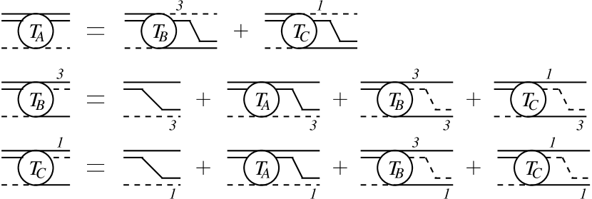
Figure 2: Coupled integral equations for $J=1/2$ $\Lambda d$ scattering. Nucleons ($\Lambda$’s) are indicated by solid (dashed) lines, respectively. The $d$ dibaryon is indicated by double solid lines, while the ${}^{3}S_{1}$ (${}^{1}S_{0}$) $\Lambda N$ dibaryon is indicated by the dashed–solid double line with index 3 (1).

The amplitude $T_{A}$ describes $J=1/2$ $\Lambda d$ scattering, while the remaining two amplitudes have a $\Lambda d$ initial state but go into the final states $(i)$ and $(ii)$ from above. Note also that there is no tree level diagram for $T_{A}$ because strangeness is conserved.

The details of the derivation of the integral equations are given in Appendix A. At a first glance, it appears that the Efimov physics known from the neutron-deuteron system Efi71 ; BHK99 ; BHK00 is not present here. The masses of the $\Lambda$ and nucleon are different and the integral equations (24) are not scale invariant for large loop momenta. However, since the $\Lambda-N$ mass difference [characterized by the ratio $y=(M_{\Lambda}-M)/(M_{\Lambda}+M)\approx 0.1$] is small, the equation becomes approximately scale invariant. Therefore, the Efimov physics will be present and can be made manifest by expanding around the limit $y=0$. The error introduced by keeping only the leading order in this expansion is at most of the order of the effective range corrections, which we neglect. Corrections to this limit can be calculated within the EFT. Setting $y=0$ in Eq. (24), we obtain:

$$T_{A}(k,p) = -\frac{1}{\pi}\int_{0}^{\Lambda_{c}}q^{2}\;dq\left\{L_{B}(p,q,E)T_{B}(k,q)-3L_{C}(p,q,E)T_{C}(k,q)\right\}$$ (6)

$$T_{B}(k,p) = -\frac{4\pi\gamma_{d}}{M}L_{I}(p,k,E)-\frac{1}{\pi}\int_{0}^{\Lambda_{c}}q^{2}\;dqL_{A}(p,q,E)T_{A}(k,q)$$

$$-\frac{1}{\pi}\int_{0}^{\Lambda_{c}}q^{2}\;dq\left\{L_{B}(p,q,E)T_{B}(k,q)+3L_{C}(p,q,E)T_{C}(k,q)\right\}$$

$$T_{C}(k,p) = \frac{4\pi\gamma_{d}}{M}L_{I}(p,k,E)+\frac{1}{\pi}\int_{0}^{\Lambda_{c}}q^{2}\;dqL_{A}(p,q,E)T_{A}(k,q)$$

$$-\frac{1}{\pi}\int_{0}^{\Lambda_{c}}q^{2}\;dq\left\{L_{B}(p,q,E)T_{B}(k,q)-L_{C}(p,q,E)T_{C}(k,q)\right\}\,,$$

where $k$ ($p$) denote the incoming (outgoing) momenta in the center-of-mass frame and $\Lambda_{c}$ is a momentum cutoff introduced to regulate the integral equations. In Eqs. (6), the outgoing momentum $p$ is taken off-shell. The total energy is $E=3k^{2}/(4M)-\gamma_{d}^{2}/M$.

In the limit $y=0$, the functions $L_{I}$ and $L_{A}$ are given by

$$L_{I}(p,k,E) = \frac{1}{pk}\ln\left(\frac{k^{2}+pk+p^{2}-ME}{k^{2}-pk+p^{2}-ME}\right)\,,$$ (7)

$$L_{A}(p,q,E) = \frac{1}{pq}\ln\left(\frac{q^{2}+pq+p^{2}-ME}{q^{2}-pq+p^{2}-ME}\right)\left[-\gamma_{d}+\sqrt{\frac{3}{4}q^{2}-ME-i\epsilon}\right]^{-1}\,.$$

$L_{B}$ ($L_{C}$) are identical to $L_{A}$ with $\gamma_{d}$ replaced by $\gamma_{3}$ ($\gamma_{1}$), respectively. The amplitude $T_{A}(p,k)$ is normalized such that

$$T_{A}(k,k)=\frac{3\pi}{M}\frac{1}{k\cot\delta-ik}\,,$$ (8)

with $\delta$ the elastic $\Lambda d$ scattering phase shift.

The integral equations (6) show the same feature as in the case of $J=1/2$ neutron-deuteron-scattering or three spinless bosons BHK99 ; BHK00 . Without the cutoff $\Lambda_{c}$, their solution would not be unique DaL63 . The origin of this nonuniqueness can be understood by solving Eq. (6) for asymptotically large off-shell momenta $\Lambda_{c}\gg q\gg\gamma_{d}\sim k$. In the asymptotic limit, the inhomogeneous terms can be neglected and the equations become independent of $k$,

$$\widetilde{T}_{A}(p) = -\frac{2}{\sqrt{3}\pi}\int_{0}^{\infty}\frac{dq}{q}\ln\left(\frac{p^{2}+pq+q^{2}}{p^{2}-pq+q^{2}}\right)\left\{\widetilde{T}_{B}(q)-3\widetilde{T}_{C}(q)\right\}$$ (9)

$$\widetilde{T}_{B}(p) = -\frac{2}{\sqrt{3}\pi}\int_{0}^{\infty}\frac{dq}{q}\ln\left(\frac{p^{2}+pq+q^{2}}{p^{2}-pq+q^{2}}\right)\left\{\widetilde{T}_{A}(q)+\widetilde{T}_{B}(q)+3\widetilde{T}_{C}(q)\right\}$$

$$\widetilde{T}_{C}(p) = +\frac{2}{\sqrt{3}\pi}\int_{0}^{\infty}\frac{dq}{q}\ln\left(\frac{p^{2}+pq+q^{2}}{p^{2}-pq+q^{2}}\right)\left\{\widetilde{T}_{A}(q)-\widetilde{T}_{B}(q)+\widetilde{T}_{C}(q)\right\}\,,$$

where we have defined $\widetilde{T}_{j}(p)=p\,T_{j}(k\sim\gamma_{d},p)$ for $j\in\{A,B,C\}$. Note that the asymptotic equations do not determine the overall normalization of the amplitudes, which will be given from matching to the low-energy solution of the full equation. The following discussion, however, is independent of this normalization. We can decouple the equations by defining a new set of amplitudes $T_{1}$, $T_{2}$, and $T_{3}$ via

$$\left(\begin{array}[]{c}{\displaystyle\widetilde{T}_{A}}\\ {\displaystyle\widetilde{T}_{B}}\\ {\displaystyle\widetilde{T}_{C}}\end{array}\right)=\left(\begin{array}[]{ccc}{\displaystyle 0}&{\displaystyle-1-\sqrt{5}}&{\quad\displaystyle-1+\sqrt{5}}\\ {\displaystyle 3}&{\displaystyle-1}&{\quad\displaystyle-1}\\ {\displaystyle 1}&{\displaystyle 1}&{\quad\displaystyle 1}\end{array}\right)\;\left(\begin{array}[]{c}{\displaystyle T_{1}}\\ {\displaystyle T_{2}}\\ {\displaystyle T_{3}}\end{array}\right)\,.$$ (10)

The new amplitudes $T_{1}$, $T_{2}$, and $T_{3}$ fulfill the equations

$$T_{1}(p) = -\frac{4}{\sqrt{3}\pi}\int_{0}^{\infty}\frac{dq}{q}\ln\left(\frac{p^{2}+pq+q^{2}}{p^{2}-pq+q^{2}}\right)T_{1}(q)$$ (11)

$$T_{2}(p) = \frac{4}{\sqrt{3}\pi}\frac{1-\sqrt{5}}{2}\int_{0}^{\infty}\frac{dq}{q}\ln\left(\frac{p^{2}+pq+q^{2}}{p^{2}-pq+q^{2}}\right)T_{2}(q)$$

$$T_{3}(p) = \frac{4}{\sqrt{3}\pi}\frac{1+\sqrt{5}}{2}\int_{0}^{\infty}\frac{dq}{q}\ln\left(\frac{p^{2}+pq+q^{2}}{p^{2}-pq+q^{2}}\right)T_{3}(q)\,.$$

All three equations are scale invariant and symmetric under the inversion $q\to 1/q$. In Ref. DaL63 , it was shown that an equation of the type

$$f(p)=\frac{4\lambda}{\sqrt{3}\pi}\int_{0}^{\infty}\frac{dq}{q}\ln\left(\frac{p^{2}+pq+q^{2}}{p^{2}-pq+q^{2}}\right)f(q)$$ (12)

has a unique solution in the form of a power law if $\lambda<\lambda_{c}=3\sqrt{3}/(4\pi)\approx 0.4135$ (see also Refs. BHK99 ; BHK00 ). This condition is clearly satisfied for the first two equations. The equation for $T_{3}$, however, has $\lambda=(1+\sqrt{5})/2\approx 1.62$. As a consequence, there are two linearly independent complex solutions $T_{3}(k,p)=p^{\pm is_{1}}$, where $s_{1}=1.35322$. The relative phase between these two solutions is not determined by Eq. (11). For a finite cutoff $\Lambda_{c}$ this phase is fixed but strongly depends on $\Lambda_{c}$. This $\Lambda_{c}$ dependence can absorbed by adding a one-parameter three-body force in the equation for $T_{3}$,

$$T_{3}(p)=\frac{4}{\sqrt{3}\pi}\frac{1+\sqrt{5}}{2}\int_{0}^{\Lambda_{c}}\frac{dq}{q}\left\{\ln\left(\frac{p^{2}+pq+q^{2}}{p^{2}-pq+q^{2}}\right)+2H(\Lambda_{c})\frac{pq}{\Lambda_{c}^{2}}\right\}T_{3}(q)\,,$$

where $H(\Lambda_{c})$ is a dimensionless function of the cutoff. In Refs. BHK99 ; BHK00 , it was shown that if the three-body force runs with cutoff as

$$H(\Lambda_{c})=-\frac{\sin(s_{1}\ln({\Lambda_{c}}/{\Lambda_{*}})-{\rm arctg}(1/s_{1}))}{\sin(s_{1}\ln({\Lambda_{c}}/{\Lambda_{*}})+{\rm arctg}(1/s_{1}))}\,,$$ (13)

all low-energy observables are independent of $\Lambda_{c}$. The renormalization group evolution of $H(\Lambda_{c})$ is governed by a limit cycle. In particular, if the cutoff is increased by a factor of $\exp(\pi/s_{1})\approx 10.2$, $H(\Lambda_{c})$ returns to its original value. $\Lambda_{*}$ is a dimensionful parameter that determines the asymptotic phase of the off-shell amplitude BHK99 ; BHK00 . It has to be fixed from a three-body observable. Once its value is known, all other observables can be predicted. Note, however, that $\Lambda_{*}$ is only determined up to factors of $\exp(\pi/s_{1})$.

Formally, the three-body force term is obtained by adding a nonderivative three-body contact term to the effective Lagrangian (II). The form of this term can be determined by starting from a general structure and matching the unknown coefficients to reproduce Eq. (III). The exact expression for this three-body term is given in Appendix B. It is interesting to note that the value $s_{1}\approx 1.35$ differs from $s_{0}\approx 1.006$ which characterizes the three-nucleon force in the triton channel BHK00 . This does not lead to a contradiction because the hypertriton channel ($I=0$) and the triton channel ($I=1/2$) have different isospin.

For the numerical studies, it is useful to write a renormalized integral equation by choosing a special cutoff,

$$\Lambda_{n} = \Lambda_{*}\exp\left[\frac{1}{s_{1}}\left(n\pi+\arctan\left(\frac{1}{s_{1}}\right)\right)\right]\,,$$ (14)

with $n>0$ an integer, at which the the three-body term proportional to $H$ in Eq. (III) vanishes HaM01 . This procedure does not remove the dependence on the three-body parameter $\Lambda_{*}$ but rather moves its dependence into the cutoff. All observables are independent of $n$, but it should be chosen such that $\Lambda_{n}\gg\gamma_{d}$ and finite cutoff corrections of order $\gamma_{d}/\Lambda_{n}$ can be neglected. In the following, we will be using Eqs. (6) with $\Lambda_{c}=\Lambda_{1}$. The $\Lambda d$ scattering amplitude is obtained by numerically solving Eqs. (6) for the desired value of the total energy. The hypertriton binding energy can be extracted by solving Eqs. (6) for negative energies and locating the position of the bound state pole in $T_{A}$.

IV Results

In order to apply the EFT to the $\Lambda NN$ system, we have to fix the parameters in Eqs. (6). The deuteron binding momentum $\gamma_{d}=45.68$ MeV is known very well. As mentioned above, the low-energy parameters for the $\Lambda N$ S-waves cannot be extracted unambiguously from a model-independent analysis of low-energy scattering data Ale68 ; Sec68 . It is known, however, that the $\Lambda N$ system is unbound, which requires $\gamma_{1}$ and $\gamma_{3}$ to be negative. The errors in the low-energy parameters extracted from extrapolations using hyperon-nucleon interaction potentials NRS73 ; RSY99 ; HHS89 ; RHS94 are not well known and can only be estimated from the variation with different potentials. Therefore, we do not take the extracted parameters as input. Rather, we vary the $\Lambda N$ pole momenta over the range of validity of the EFT and study the implications on the hypertriton and $\Lambda d$ scattering.

In principle, we have three unknown parameters: $\gamma_{1}$, $\gamma_{3}$, and the three-body parameter $\Lambda_{*}$. However, we will first address the simpler scenario $\gamma_{1}=\gamma_{3}$, which follows from the $SU(6)$ spin-flavor symmetry of the quark model AkD65 ; BaR65 . Such an $SU(6)$ symmetry also emerges in the large-$N_{c}$ limit of QCD KaS96 . Symmetry violating corrections are suppressed by $1/N_{c}$ and the strange quark mass. Since both isospin and strangeness of the ${}^{3}S_{1}$ and ${}^{1}S_{0}$ $\Lambda N$ partial waves are the same, the difference between $\gamma_{1}$ and $\gamma_{3}$ is a pure spin splitting effect. In most hyperon-nucleon potentials this effect is of the order 30% NRS73 ; RSY99 ; HHS89 ; RHS94 . Neglecting this splitting leaves us with two parameters: $\gamma_{i}(=\gamma_{1}=\gamma_{3})$ and $\Lambda_{*}$. In the following, we vary these two parameters and study the constraints that follow from a correct description of the hypertriton. We will also elucidate the consequences for $\Lambda d$ scattering.

First, we study the constraints on the parameters $\gamma_{i}$ and $\Lambda_{*}$ by the requirement that the hypertriton binding energy be reproduced. An interesting question is whether there are certain values of $\gamma_{i}$ and $\Lambda_{*}$ that are incompatible with the hypertriton data. Furthermore, it is possible that the approximation $\gamma_{1}=\gamma_{3}$ proves too restrictive. In Fig. 3, we plot $\Lambda_{*}$ as a function of $\gamma_{i}$ with the

Figure 3: Values of $\Lambda_{*}/\gamma_{d}$ and $\gamma_{i}/\gamma_{d}$ that lead to the correct binding energy for the hypertriton.

requirement that the hypertriton binding energy is reproduced. We vary $\gamma_{i}$ from $0$ to $-2\gamma_{d}$, which is about where corrections of ${\cal O}(QR)$ are expected to become important. Positive values of $\gamma_{i}$ are excluded because the $\Lambda N$ system is not bound. All allowed values fall on a curve with a linear dependence on $\gamma_{i}$,

$$\Lambda_{*}/\gamma_{d}=1.08-0.55\gamma_{i}/\gamma_{d}\,.$$ (15)

For every value of $\gamma_{i}$ in the interval a corresponding value of $\Lambda_{*}$ that reproduces the hypertriton can be found. Clearly, the exact value of $\gamma_{i}$ and therefore the $\Lambda N$ scattering lengths cannot be determined from the hypertriton binding energy. This is in contrast to Ref. CJF97 , where it was found that with standard hyperon-nucleon potentials, the correct binding energy for the hypertriton cannot be reproduced if the singlet $\Lambda N$ scattering length differs more than 10% from 1.85 fm.

In Fig. 4, we compare the scattering phase shifts for $\Lambda d$ scattering in the hypertriton channel for different points on the curve in Fig. 3. Fig. 4 shows three curves with $\gamma_{i}$ chosen to be equal in magnitude to $\gamma_{d}$ as well as a factor of two smaller and larger. The phase shifts agree very well for small momenta around threshold and begin to differ slightly close to the deuteron breakup threshold. This implies that low-energy $\Lambda d$ scattering does not give additional constraints for the values of $\gamma_{i}$ and $\Lambda_{*}$. Consequently, neither the hypertriton binding energy nor the low-energy $\Lambda d$ phase shifts can be used to fix the exact value of $\gamma_{i}$. Such information can only come from low-energy $\Lambda N$ scattering.

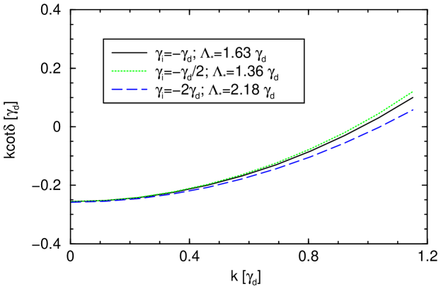
Figure 4: $\Lambda d$ scattering phase shifts for different values of $\gamma_{i}$ and $\Lambda_{*}$ that lead to the correct hypertriton binding energy (all quantities in units of $\gamma_{d}$).

On the other hand, this observation allows for a prediction of the low-energy $\Lambda d$ phase shifts [given by the curves in Fig. 4] independent of the exact values for $\gamma_{i}$ and $\Lambda_{*}$. This is a direct consequence of the shallowness of the hypertriton. Extracting the low-energy doublet $\Lambda d$ scattering parameters from the phase shifts, we find for the scattering length $a_{\Lambda d}$ and effective range $r_{\Lambda d}$:

$$a_{\Lambda d}=(16.8^{+4.4}_{-2.4})\mbox{ fm}\qquad\mbox{and}\qquad r_{\Lambda d}=(2.3\pm 0.3)\mbox{ fm}\,,$$ (16)

where the errors are due to the uncertainty in the hypertriton binding energy. Our value for the scattering length is in good agreement with Ref. CJF97 , while the effective range is about 1 fm smaller.

It is also interesting to look at the “Phillips line”, which describes the correlation between the $\Lambda d$ scattering length $a_{\Lambda d}$ and the hypertriton binding energy $B_{3}^{\Lambda}$. The Phillips line was observed in the neutron-deuteron system, where the results of calculations of the doublet $nd$ scattering length and the triton binding energy using different $NN$ potentials fall on a line when plotted in a plane Phi68 . A similar line exists for the hypertriton (cf. Fig. 7 in Ref. FeJ01 ). In the EFT framework, the Phillips line is parametrized by variations in the three-body parameter $\Lambda_{*}$ BHK99 ; BHK00 . In Fig. 5, we show the

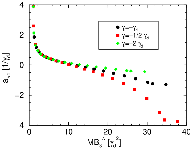
Figure 5: Phillips line for different values of $\gamma_{i}$ (all quantities in units of $\gamma_{d}$).

Phillips line for the three values of $\gamma_{i}$ from Fig. 4. For small $B_{3}^{\Lambda}$, the different Phillips lines coincide exactly (the physical hypertriton corresponds to $MB_{3}^{\Lambda}\approx 1.06\,\gamma_{d}^{2}$) and deviate from each other only at extremely large binding energies. However, the EFT is expected to break down when the three-body binding momentum $\gamma_{3}^{\Lambda}$ from Eq. (1) becomes of the order of the pion mass. This is the case for $MB_{3}^{\Lambda}\hskip 1.99997pt\raisebox{2.15277pt}{$>$}\raisebox{-3.00003pt}{$\sim$}\hskip 1.99997pt8\gamma_{d}^{2}$. Consequently, the region where the Phillips lines differ is unphysical. For all practical purposes the Phillips line is independent of $\gamma_{i}$.

The characteristic momentum that sets the scale of corrections to the large-scattering-length approximation is given by the binding momentum of the hypertriton. Using the measured value for $B_{3}^{\Lambda}$ and Eq. (1), we obtain $\gamma_{3}^{\Lambda}\approx 0.3\,\gamma_{d}$. This momentum can be used to estimate the contribution of the effective range term in the two-body amplitudes which is the leading correction at ${\cal O}(QR)$. For our approximation to be accurate, we need $|\gamma|\gg|r(\gamma_{3}^{\Lambda})^{2}/2|$ in each of the two-body partial waves. Since $(\gamma_{3}^{\Lambda})^{2}/2\approx 0.05\,\gamma_{d}^{2}$ is extremely small, the effective range term gives only a small correction even when the scattering length and effective range are of the same order.

We have also studied the more general case $\gamma_{1}\neq\gamma_{3}$. The conclusions in this case are unchanged: requiring the correct binding energy of the hypertriton does not constrain the specific values of $\gamma_{1}$ and $\gamma_{3}$ as long as they are within the range of validity of the EFT ($0>\gamma_{1},\gamma_{3}\hskip 1.99997pt\raisebox{2.15277pt}{$>$}\raisebox{-3.00003pt}{$\sim$}\hskip 1.99997pt-2\gamma_{d}$). The results for $\Lambda d$ scattering confirm Fig. 4 and Eq. (16).

The insensitivity to the precise values of $\gamma_{1}$ and $\gamma_{3}$ and the small separation energy of the hypertriton into a deuteron and a $\Lambda$ ($B^{\Lambda}=0.13$ MeV) can be exploited even further: it is possible to write an EFT with only deuterons and $\Lambda$’s as degrees of freedom Bira01 . Effects from the deuteron structure and $\Lambda N$ interaction can be included perturbatively via local operators.

To summarize, we have discussed the hypertriton and doublet $\Lambda d$ scattering in an EFT for large two-body scattering lengths. Due to the small binding energy of the hypertriton, our analysis is expected to hold even if the $\Lambda N$ low-energy parameters are ${\cal O}(1/m_{\pi})$ as extracted from potential models. As in the triton case, consistent renormalization requires a one-parameter three-body force at leading order whose renormalization group evolution is governed by a limit cycle. The period of the limit cycle $\exp(\pi/s_{1})\approx 10.2$ is a factor two smaller than for the triton. In contrast to standard potential models where the binding energy of the hypertriton is very sensitive to the singlet $\Lambda N$ scattering length CJF97 , the three-body force can always compensate for changes in the low-energy $\Lambda N$ parameters. While the $\Lambda N$ low-energy parameters cannot be fixed by requiring the correct binding energy for the hypertriton, the shallowness of the hypertriton still allows for a unique prediction of low-energy doublet $\Lambda d$ scattering. Using the experimental binding energy of the hypertriton as input, we find for the scattering length $a_{\Lambda d}=(16.8^{+4.4}_{-2.4})$ fm and for the effective range $r_{\Lambda d}=(2.3\pm 0.3)$ fm. In the future, it would be interesting to go to higher orders and apply EFT methods to a wider class of observables and other halo nuclei. Work in this direction is in progress BHK01 .

Appendix A Derivation of three-body equation

In this Appendix, we give some details of the derivation of the integral equation (6) for the general case $M_{\Lambda}\neq M$. From the Lagrangian (II) and the Feynman diagrams in Fig. 2, we obtain

$$t_{A}^{ij}(\vec{k},\vec{p})_{\alpha\beta} = g_{d}g_{3}\int\frac{d^{3}q}{(2\pi)^{3}}\;t_{B}^{ik}(\vec{k},\vec{q})_{\alpha\gamma}\,\frac{(\sigma_{j}\sigma_{k})_{\gamma\beta}\;D_{3}(E-\frac{q^{2}}{2M},\vec{q})}{E-\frac{p^{2}}{2M_{\Lambda}}-\frac{q^{2}}{2M}-\frac{(\vec{q}+\vec{p})^{2}}{2M}+i\epsilon}$$

$$+g_{d}g_{1}\int\frac{d^{3}q}{(2\pi)^{3}}\;t_{C}^{i}(\vec{k},\vec{q})_{\alpha\gamma}\,\frac{(\sigma_{j})_{\gamma\beta}\;D_{1}(E-\frac{q^{2}}{2M},\vec{q})}{E-\frac{p^{2}}{2M_{\Lambda}}-\frac{q^{2}}{2M}-\frac{(\vec{q}+\vec{p})^{2}}{2M}+i\epsilon}$$

$$t_{B}^{ij}(\vec{k},\vec{p})_{\alpha\beta} = -2g_{d}g_{3}\frac{(\sigma_{j}\sigma_{i})_{\alpha\beta}}{E-\frac{k^{2}}{2M_{\Lambda}}-\frac{p^{2}}{2M}-\frac{(\vec{k}+\vec{p})^{2}}{2M}+i\epsilon}$$

$$+2g_{d}g_{3}\int\frac{d^{3}q}{(2\pi)^{3}}\;t_{A}^{ik}(\vec{k},\vec{q})_{\alpha\gamma}\,\frac{(\sigma_{j}\sigma_{k})_{\gamma\beta}\;D_{d}(E-\frac{q^{2}}{2M_{\Lambda}},\vec{q})}{E-\frac{p^{2}}{2M}-\frac{q^{2}}{2M_{\Lambda}}-\frac{(\vec{q}+\vec{p})^{2}}{2M}+i\epsilon}$$

$$+g_{3}^{2}\int\frac{d^{3}q}{(2\pi)^{3}}\;t_{B}^{ik}(\vec{k},\vec{q})_{\alpha\gamma}\,\frac{(\sigma_{j}\sigma_{k})_{\gamma\beta}\;D_{3}(E-\frac{q^{2}}{2M},\vec{q})}{E-\frac{p^{2}+q^{2}}{2M}-\frac{(\vec{q}+\vec{p})^{2}}{2M_{\Lambda}}+i\epsilon}$$

$$-g_{1}g_{3}\int\frac{d^{3}q}{(2\pi)^{3}}\;t_{C}^{i}(\vec{k},\vec{q})_{\alpha\gamma}\,\frac{(\sigma_{j})_{\gamma\beta}\;D_{1}(E-\frac{q^{2}}{2M},\vec{q})}{E-\frac{p^{2}+q^{2}}{2M}-\frac{(\vec{q}+\vec{p})^{2}}{2M_{\Lambda}}+i\epsilon}$$

$$t_{C}^{i}(\vec{k},\vec{p})_{\alpha\beta} = -2g_{d}g_{1}\frac{(\sigma_{i})_{\alpha\beta}}{E-\frac{k^{2}}{2M_{\Lambda}}-\frac{p^{2}}{2M}-\frac{(\vec{k}+\vec{p})^{2}}{2M}+i\epsilon}$$

$$+2g_{d}g_{1}\int\frac{d^{3}q}{(2\pi)^{3}}\;t_{A}^{ik}(\vec{k},\vec{q})_{\alpha\gamma}\,\frac{(\sigma_{k})_{\gamma\beta}\;D_{d}(E-\frac{q^{2}}{2M_{\Lambda}},\vec{q})}{E-\frac{p^{2}}{2M}-\frac{q^{2}}{2M_{\Lambda}}-\frac{(\vec{q}+\vec{p})^{2}}{2M}+i\epsilon}$$

$$-g_{1}g_{3}\int\frac{d^{3}q}{(2\pi)^{3}}\;t_{B}^{ik}(\vec{k},\vec{q})_{\alpha\gamma}\,\frac{(\sigma_{k})_{\gamma\beta}\;D_{3}(E-\frac{q^{2}}{2M},\vec{q})}{E-\frac{p^{2}+q^{2}}{2M}-\frac{(\vec{q}+\vec{p})^{2}}{2M_{\Lambda}}+i\epsilon}$$

$$+g_{1}^{2}\int\frac{d^{3}q}{(2\pi)^{3}}\;t_{C}^{i}(\vec{k},\vec{q})_{\alpha\gamma}\,\frac{\delta_{\gamma\beta}\;D_{1}(E-\frac{q^{2}}{2M},\vec{q})}{E-\frac{p^{2}+q^{2}}{2M}-\frac{(\vec{q}+\vec{p})^{2}}{2M_{\Lambda}}+i\epsilon}\,,$$

where $i,j,k$ are vector indices and $\alpha,\beta,\gamma$ are spinor indices in spin space. $k(p)$ are the incoming (outgoing) momenta in the center-of-mass frame and $E=k^{2}/(4M)-\gamma_{d}^{2}/M+k^{2}/(2M_{\Lambda})$ is the total energy. The momentum $p$ is taken off-shell. The isospin dependence of the amplitudes $t_{B}$ and $t_{C}$ has been absorbed into the amplitudes via the definition

$$t_{B}^{ij}(\vec{k},\vec{p})_{\alpha\beta} = t_{B}^{ij}(\vec{k},\vec{p})_{\alpha\beta}^{eb}(\tau_{2})_{be}\,,$$ (20)

and similarly for $t_{C}$, where $e,b$ are isospinor indices. Next we project onto total angular momentum $J=1/2$ by using the definitions

$$t_{A/B}(\vec{k},\vec{p})\,\delta_{\alpha\beta} = \frac{1}{3}(\sigma_{i})_{\alpha\alpha^{\prime}}t_{A/B}^{ij}(\vec{k},\vec{p})_{\alpha^{\prime}\beta^{\prime}}(\sigma_{j})_{\beta^{\prime}\beta}$$ (21)

$$t_{C}(\vec{k},\vec{p})\,\delta_{\alpha\beta} = \frac{1}{3}(\sigma_{i})_{\alpha\alpha^{\prime}}t_{C}^{i}(\vec{k},\vec{p})_{\alpha^{\prime}\beta}\,,$$

and projecting on relative S-waves. We also have to account for the wave function renormalization of the deuteron,

$$Z_{d}^{-1}=i\frac{\partial}{\partial p_{0}}\left.(iD_{d}(p_{0},\vec{p}))^{-1}\right|_{p_{0}=-\gamma_{d}^{2}/M,\,\vec{p}=0}=\frac{M^{2}g_{d}^{2}}{4\pi\gamma_{d}}\,.$$ (22)

Defining

$$T_{A}(k,p) = Z_{d}t_{A}(k,p)$$ (23)

$$T_{B}(k,p) = Z_{d}\frac{g_{d}}{g_{3}}t_{B}(k,p)$$

$$T_{C}(k,p) = Z_{d}\frac{g_{d}}{g_{1}}t_{C}(k,p)\,,$$

we finally obtain the integral equations

$$T_{A}(k,p) = -\frac{1}{\pi(1-y)}\int_{0}^{\Lambda_{c}}q^{2}\;dq\left\{\widetilde{L}_{B}(p,q,E)T_{B}(k,q)-3\widetilde{L}_{C}(p,q,E)T_{C}(k,q)\right\}$$ (24)

$$T_{B}(k,p) = -\frac{4\pi\gamma_{d}}{M}L_{I}(p,k,E)-\frac{1}{\pi}\int_{0}^{\Lambda_{c}}q^{2}\;dqL_{A}(p,q,E)T_{A}(k,q)$$

$$-\frac{1}{\pi(1-y)}\int_{0}^{\Lambda_{c}}q^{2}\;dq\left\{L_{B}(p,q,E)T_{B}(k,q)+3L_{C}(p,q,E)T_{C}(k,q)\right\}$$

$$T_{C}(k,p) = \frac{4\pi\gamma_{d}}{M}L_{I}(p,k,E)+\frac{1}{\pi}\int_{0}^{\Lambda_{c}}q^{2}\;dqL_{A}(p,q,E)T_{A}(k,q)$$

$$-\frac{1}{\pi(1-y)}\int_{0}^{\Lambda_{c}}q^{2}\;dq\left\{L_{B}(p,q,E)T_{B}(k,q)-L_{C}(p,q,E)T_{C}(k,q)\right\}$$

where $\Lambda_{c}$ is a momentum cutoff and $y=(M_{\Lambda}-M)/(M_{\Lambda}+M)\approx 0.1$ characterizes the $\Lambda-N$ mass difference. The functions $L_{I}$, $L_{A}$, $L_{B}$, and $\widetilde{L}_{B}$ are given by

$$L_{I}(p,k,E) = \frac{1}{pk}\ln\left(\frac{k^{2}/(1+y)+pk+p^{2}-ME}{k^{2}/(1+y)-pk+p^{2}-ME}\right)\,,$$ (25)

$$L_{A}(p,q,E) = \frac{1}{pq}\ln\left(\frac{q^{2}/(1+y)+pq+p^{2}-ME}{q^{2}/(1+y)-pq+p^{2}-ME}\right)$$

$$\times\left[-\gamma_{d}+\sqrt{q^{2}\,(3-y)/(1+y)/4-ME-i\epsilon}\right]^{-1}\,,$$

$$L_{B}(p,q,E) = \frac{1}{pq}\ln\left(\frac{q^{2}+p^{2}+pq(1-y)-ME(1+y)}{q^{2}+p^{2}-pq(1-y)-ME(1+y)}\right)$$

$$\times\left[-\gamma_{3}+\sqrt{q^{2}\left(3+2y-y^{2}\right)/4-ME(1+y)-i\epsilon}\right]^{-1}\,,$$

$$\widetilde{L}_{B}(p,q,E) = \frac{1}{pq}\ln\left(\frac{q^{2}+pq+p^{2}/(1+y)-ME}{q^{2}-pq+p^{2}/(1+y)-ME}\right)$$

$$\times\left[-\gamma_{3}+\sqrt{q^{2}\left(3+2y-y^{2}\right)/4-ME(1+y)-i\epsilon}\right]^{-1}\,.$$

$L_{C}$ $(\widetilde{L}_{C})$ is identical to $L_{B}$ $(\widetilde{L}_{B})$ with $\gamma_{3}$ replaced by $\gamma_{1}$.

Appendix B Three-body force term

The three-body term proportional to $H(\Lambda_{c})$ in Eq. (III) can be obtained by adding a local, nonderivative three-body contact term to the Lagrangian (II). This term is most easily determined by starting from a general structure and matching the coefficients of the individual terms to reproduce the three-body term in Eq. (III). This leads to,

$${\cal L}_{3} = \frac{MH(\Lambda_{c})}{20\Lambda_{c}^{2}}\bigg{\{}16\sqrt{5}\,g_{d}^{2}\left[d_{l}^{*}\Lambda_{\alpha}(\sigma_{l}\sigma_{l^{\prime}})_{\alpha\beta}\Lambda^{*}_{\beta}d_{l^{\prime}}\right]$$

$$- (5+3\sqrt{5})\left(g_{3}^{2}\left[(u^{3}_{l})^{*}_{a}N_{\alpha a}(\sigma_{l}\sigma_{l^{\prime}})_{\alpha\beta}N^{*}_{\beta b}(u^{3}_{l^{\prime}})_{b}\right]-3g_{1}^{2}\left[(u^{1})^{*}_{a}N_{\alpha a}N^{*}_{\beta b}(u^{1})_{b}\right]\right)$$

$$+ 2(5+\sqrt{5})g_{d}g_{3}\left[d_{l}^{*}N_{\alpha a}(\sigma_{l}\sigma_{l^{\prime}})_{\alpha\beta}\Lambda^{*}_{\beta}(\tau_{2})_{ab}(u^{3}_{l^{\prime}})_{b}+\mbox{H.c.}\right]$$

$$- (5+3\sqrt{5})g_{1}g_{3}\left[(u^{3}_{l})^{*}_{a}N_{\alpha a}(\sigma_{l})_{\alpha\beta}N^{*}_{\beta b}(u^{1})_{b}+\mbox{H.c.}\right]$$

$$+ 2(5+\sqrt{5})g_{d}g_{1}\left[d_{l}^{*}N_{\alpha a}(\sigma_{l})_{\alpha\beta}\Lambda^{*}_{\beta}(\tau_{2})_{ab}(u^{1})_{b}+\mbox{H.c.}\right]\bigg{\}}\,,$$

where $\alpha,\beta$ ($a,b$) are spinor (isospinor) indices and $l,l^{\prime}$ are vector indices. Eq. (B) represents a contact three-body force written in terms of dibaryon, nucleon, and $\Lambda$ fields but to leading order is equivalent to a three-baryon contact force. This becomes obvious if the dibaryon fields are integrated out by performing a Gaussian path integral BHK99 ; BHK00 ; GBG00 .

References

- (1) S. Weinberg, Phys. Lett. B 251, 288 (1990); Nucl. Phys. B 363, 3 (1991).
- (2) Nuclear Physics with Effective Field Theory II, ed. P.F. Bedaque, M.J. Savage, R. Seki, and U. van Kolck (World Scientific, Singapore, 1999).
- (3) Nuclear Physics with Effective Field Theory, ed. R. Seki, U. van Kolck, and M.J. Savage (World Scientific, Singapore, 1998).
- (4) U. van Kolck, Prog. Part. Nucl. Phys. 43, 409 (1999).
- (5) S.R. Beane, P.F. Bedaque, W.C. Haxton, D.R. Phillips, and M.J. Savage, [nucl-th/0008064].
- (6) G.P. Lepage, in From Actions to Answers, TASI’89, ed. T. DeGrand and D. Toussaint (World Scientific, Singapore, 1990); [nucl-th/9706029]; D.B. Kaplan, [nucl-th/9506035].
- (7) U. van Kolck, Nucl. Phys. A 645, 273 (1999).
- (8) D.B. Kaplan, M.J. Savage, and M.B. Wise, Phys. Lett. B 424, 390 (1998); Nucl. Phys. B 534, 329 (1998).
- (9) J.-W. Chen, G. Rupak, and M.J. Savage, Nucl. Phys. A 653, 386 (1999).
- (10) S.R. Beane and M.J. Savage, [nucl-th/0011067].
- (11) P.F. Bedaque and U. van Kolck, Phys. Lett. B 428, 221 (1998).
- (12) P.F. Bedaque, H.-W. Hammer, and U. van Kolck, Phys. Rev. C 58, R641 (1998).
- (13) P.F. Bedaque and H.W. Grießhammer, Nucl. Phys. A 671, 357 (2000).
- (14) F. Gabbiani, P.F. Bedaque, and H.W. Grießhammer, Nucl. Phys. A 675, 601 (2000).
- (15) G. Rupak and X.-W. Kong, [nucl-th/0108059].
- (16) P.F. Bedaque, H.-W. Hammer, and U. van Kolck, Phys. Rev. Lett. 82, 463 (1999); Nucl. Phys. A 646, 444 (1999).
- (17) P.F. Bedaque, H.-W. Hammer, and U. van Kolck, Nucl. Phys. A 676, 357 (2000).
- (18) B. Blankleider and J. Gegelia, [nucl-th/0009007]; [nucl-th/0107043].
- (19) H.-W. Hammer and T. Mehen, Nucl. Phys. A 690, 535 (2001).
- (20) H.-W. Hammer and T. Mehen, Phys. Lett. B 516, 353 (2001).
- (21) L.H. Thomas, Phys. Rev. 47, 903 (1935).
- (22) A.C. Phillips, Nucl. Phys. A 107, 209 (1968).
- (23) V.N. Efimov, Sov. J. Nucl. Phys. 12, 589 (1971); 29, 546 (1979).
- (24) M. Juric et al., Nucl. Phys. B 52, 1 (1973).
- (25) D.H. Davis, LAMPF Workshop on () Physics, AIP Conf. Proc. 224, 38 (1991).
- (26) R.B. Clare and J.S. Levinger, Phys. Rev. C 31, 2303 (1985).
- (27) I.R. Afnan and B.F. Gibson, Phys. Rev. C 40, R7 (1989); 41, 2787 (1990).
- (28) J.G. Congleton, J. Phys. G 18, 339 (1992).
- (29) K. Miyagawa and W. Glöckle, Phys. Rev. C 48, 2576 (1993).
- (30) A. Cobis, A.S. Jensen, and D.V. Fedorov, J. Phys. G 23, 401 (1997).
- (31) D.V. Fedorov and A.S. Jensen, [nucl-th/0107027].
- (32) G. Alexander et. al., Phys. Rev. 173, 1452 (1968).
- (33) B. Sechi-Zorn et. al., Phys. Rev. 175, 1735 (1968).
- (34) M.M. Nagels, T.A. Rijken, and J.J. de Swart, Ann. Phys. (NY) 79, 338 (1973).
- (35) T.A. Rijken, V.G.J. Stoks, and Y. Yamamoto, Phys. Rev. C 59, 21 (1999); V.G.J. Stoks and T.A. Rijken, Phys. Rev. C 59, 3009 (1999).
- (36) B. Holzenkamp, K. Holinde, and J. Speth, Nucl. Phys. A 500, 485 (1989).
- (37) A. Reuber, K. Holinde, and J. Speth, Nucl. Phys. A 570, 543 (1994).
- (38) C.L. Korpa, A.E.L. Dieperink, and R.G.E. Timmermans, [nucl-th/0109072].
- (39) D.B. Kaplan, Nucl. Phys. B 494, 471 (1997).
- (40) M.J. Savage, Phys. Rev. C 55, 2185 (1997).
- (41) C. Ordóñez, L. Ray, and U. van Kolck, Phys. Rev. C 53, 2086 (1996).
- (42) G.S. Danilov, Sov. Phys. JETP 13, 349 (1961).
- (43) D.A. Akyeampong and R. Delbourgo, Phys. Rev. 140, B1013 (1965).
- (44) V. Barger and M.H. Rubin, Phys. Rev. 140, B1366 (1965).
- (45) D.B. Kaplan and M.J. Savage, Phys. Lett. B 365, 244 (1996).
- (46) U. van Kolck, private communication.
- (47) C.A. Bertulani, H.-W. Hammer, and U. van Kolck, in preparation.