A kinetic approach to $\eta^{\prime}$ production from a CP-odd phase

I Introduction

Construction of the Relativistic Heavy Ion Collider (RHIC) at the Brookhaven National Laboratory is completed and it is designed to initiate energy densities sufficient to produce a quark gluon plasma (QGP) [1]. Such a strongly correlated state of matter has a life time smaller than $1fm/c$ and due to rapid collisions the plasma thermalizes, and at critical values of temperature and density the quarks and gluons form hadronic bound states: a process driven by confinement and chiral symmetry breaking. Many aspects of the plasma’s production and evolution are characterised by non-linear dynamics. The hadronisation process itself as well as critical phenomena in the vicinity of the phase boundary require a study with non-equilibrium techniques.

One challenging example of a far from equilibrium process is spontaneous particle creation in a strong background electric field, i.e. the Schwinger mechanism [2]. However, pair creation in QED has never been observed directly although planned new facilities such as a X-ray free electron laser (XFEL) [3, 4] will allow to reach the region of required critical field strengths. Therefore this non-perturbative effect was mainly studied for applications providing strong enough fields ranging from black hole quantum evaporation [5] to particle production in the early universe [6] and in ultra-relativistic heavy-ion collisions [7].

An unsolved problem of conceptual and practical interest is the precise connection between field theory and kinetic theory. Recently a link between the mean field approach of vacuum pair creation in a spatially homogeneous Abelian background field and a kinetic formulation was established in [8]. The resulting source term for spontaneous pair creation is non-Markovian and retains quantum statistical effects [9, 10]. In many approaches the background field is treated as a time dependent classical field with feedback incorporated via Maxwell’s equation, e.g. [11, 12, 13, 14, 15]. In these approaches the production of fermion/gluon pairs was employed to describe the formation of a quark-gluon plasma. Herein we focus on the production of bosonic particles in hot hadronic matter in QCD.

Lattice calculations, e.g. [16], as well as QCD Green function approaches, e.g. [15, 17], indicate that the deconfinement and chiral phase transitions are coincident [15, 18, 19, 20]. At present it is an open question whether the restoration of the U_A(1) symmetry which is broken in the QCD vacuum sets in already at the deconfinement transition temperature or above. In addition parity maybe spontaneously broken which is connected with a non-vanishing QCD $\theta$ angle [21]. The CP odd phase is of particular interest since it may have experimental signatures such as an enhanced production of $\eta$ and $\eta^{\prime}$ mesons [22, 23] which can contribute via their decays to the low mass dilepton enhancement. They can decay via CP violating processes such as ${\eta}\to{\pi}^{0}{\pi}^{0}$.

Herein we study the production of $\eta^{\prime}$- particles during the decay of the CP-odd phase. Complementary to [24] where the decay rate of metastable states was estimated, we study the full time evolution of the momentum distribution function using a kinetic description based on an effective Lagrangian. We start from the Witten- DiVecchia-Veneziano model [25], however, different approaches can be applied, e.g. [26].

In this article, the external background field concept is replaced by a potential yielding self-interaction and non-linearity. This potential dominates the solution of the quantum kinetic equation which is derived using an evolution operator approach. The introduced technique to link an effective Lagrangian and kinetic theory is not restricted to the discussed model calculation of $\eta^{\prime}$ production. It’s application is general in quantum field theory.

The article is organised as follows. In Section II we introduce the model Lagrangian and identify the self-interaction parts. In Section III we perform the quantization of the evolution operator used in Section IV to derive a quantum kinetic equation. In Sections V and VI we discuss the decay of the CP odd phase in view of our numerical results.

II The effective Lagrangian

We start from the effective Lagrangian of the Witten-DiVecchia-Veneziano model [25]

$${\cal L}_{eff} = \frac{f^{2}_{\pi}}{4}\bigg{(}tr(\partial_{\mu}U\partial_{\mu}U^{+})+tr(MU+MU^{+})$$ (2)

$$-\frac{a}{N_{c}}[\theta-\frac{i}{2}tr(\ln U-\ln U^{+})]^{2}\bigg{)},$$

which describes the low-energy dynamics of the nonet of the pseudoscalar mesons [27] in the large $N_{c}$-limit of QCD. The meson fields are described by the $N_{f}\times N_{f}$-matrix $U$ in Eq. (2). Explicit chiral symmetry breaking is realized by the current quark mass matrix $M$ with the diagonal elements related to $\pi$ and $K$ meson masses. With the parametrization $U=\exp(i\phi/f_{\pi})$, the matrix $\phi$ representing the singlet and the octet meson fields yields the pseudoscalar nonet. The last term in the effective Lagrangian is related to the $U_{A}(1)$-anomaly: the singlet is massive also in chiral limit. The parameter $a=2N_{f}\lambda_{YM}/f^{2}_{\pi}$ contains the topological susceptibility, $\lambda_{YM}$. Herein we focus on the singlet state which is the main component for $\eta^{\prime}$ and obtain the following Lagrangian:

$${\cal L}=\frac{1}{2}({\partial}_{\mu}{\eta})({\partial}^{\mu}{\eta})+f^{2}{\mu}^{2}\cos\Big{(}\frac{\eta}{f}\Big{)}-\frac{a}{2}{\eta}^{2}\,.$$ (3)

In Eq. (3) $f=\sqrt{\frac{3}{2}}f_{\pi}$, where $f_{\pi}=92$ MeV is the semi-leptonic pion decay constant, ${\mu}^{2}=\frac{1}{3}(m^{2}_{\pi}+2m^{2}_{K})$ is a parameter depending on $\pi$- and $K$-meson masses. For zero temperature $T=0$, $a=m^{2}_{\eta}+m^{2}_{{\eta}^{\prime}}-2m_{K}^{2}\simeq 0.726~{}{\rm GeV}^{2}$ and ${\mu}^{2}\simeq 0.171~{}{\rm GeV}^{2}$. In response to non-zero temperature and density mesons have an effective mass, e.g. [28]: $\mu$ and $a$ are functions of $T$ and hence the potential corresponding to (3) has modified properties close to the deconfinement phase transition.

From (3) we obtain the following Klein-Gordon type equation of motion for the field ${\eta}(\vec{x},t)$:

$$(\Box+m_{0}^{2}){\eta}=J_{s},$$ (4)

where $m_{0}^{2}\equiv a+{\mu}^{2}$. The nonlinear current

$$J_{s}\equiv-f{\mu}^{2}\Big{[}\sin\Big{(}\frac{\eta}{f}\Big{)}-\Big{(}\frac{\eta}{f}\Big{)}\Big{]}$$ (5)

contains orders ${\eta}^{3}$ and higher and is related to the self-interaction of the field $\eta$. Note that the linear term of the total current $J=-{\mu}^{2}{\eta}+J_{s}$ is contained in the mass squared term of the lelf-hand side of Eq. (4)

The total Hamiltonian density, ${\cal H}={\cal H}_{0}+{\cal H}_{s}$, is given by

$${\cal H}_{0} = \frac{1}{2}{\pi}^{2}+\frac{1}{2}(\vec{\nabla}{\eta})^{2}+\frac{1}{2}m_{0}^{2}{\eta}^{2},$$ (6)

$${\cal H}_{s} = 2f^{2}{\mu}^{2}\Big{[}{\sin}^{2}\Big{(}\frac{\eta}{2f}\Big{)}-\Big{(}\frac{\eta}{2f}{\Big{)}}^{2}\Big{]},$$ (7)

where ${\cal H}_{0}$ involves only the free field part with the mass $m_{0}$; ${\cal H}_{s}$ includes self interaction starting at orders $\eta^{4}$ and ${\pi}$ is the momentum canonically conjugate to $\eta$:

$${\pi}(\vec{x},t)=\dot{\eta}(\vec{x},t),$$ (8)

where the overdot denotes the derivative with respect to time.

III Evolution operator approach

We introduce the in-field, ${\eta}_{in}(\vec{x},t)$, as a solution of Eq. (4) in absence of sources and quantise it according to the standard canonical procedure (see Appendix A). The original self-interacting field is connected with the in-field by the unitary transformation:

$${\eta}(\vec{x},t)=U^{-1}(t){\eta}_{in}(\vec{x},t)U(t),$$ (9)

where

$$U(t)\equiv T\exp\{-i\int_{-\infty}^{t}dt^{\prime}H_{s}^{in}(t^{\prime})\}$$ (10)

is the time evolution operator with the self-interaction Hamiltonian written in terms of the in-field operators

$$H_{s}^{in}\equiv\int d^{3}x{\cal H}_{s}({\eta}={\eta}_{in};{\pi}={\pi}_{in})\,.$$ (11)

In the limit $t\to-\infty$ we have $U(t)\to I$, so that

$$\lim_{t\to-\infty}{\eta}(\vec{x},t)={\eta}_{in}(\vec{x},t).$$ (12)

The exact meaning of (12) depends on details of the current $J_{s}$ which in our model is determined by self-interaction taking place at all times. Hence Eq. (12) is a priori difficult to justify. We assume an adiabatic vanishing of the interaction for $t\to-\infty$.

The field ${\eta}(\vec{x},t)$ is given by the space-homogeneous mean value ${\phi}(t)=\langle{\eta}(\vec{x},t)\rangle$ and fluctuations ${\chi}$

$${\eta}(\vec{x},t)={\phi}(t)+{\chi}(\vec{x},t)$$ (13)

with $\langle{\chi}(\vec{x},t)\rangle=0$. Assuming that ${\chi}\ll f$, quantum fluctuations can be treated perturbatively. Herein we restrict ourselves to zeroth ⁽⁰⁾ and first ⁽¹⁾ order. Substituting Eq. (13) into Eq. (4) yields

$$(\Box+m_{0}^{2}){\chi}+\ddot{\phi}+m_{0}^{2}{\phi}=J_{s}^{(1)},$$ (14)

where

$$J_{s}^{(1)}\equiv J_{s}^{(0)}+{\mu}^{2}\Big{[}1-\cos\Big{(}\frac{\phi}{f}\Big{)}\Big{]}{\chi}.$$ (15)

The zeroth order of the current is given by

$$J_{s}^{(0)}\equiv-f{\mu}^{2}\Big{[}\sin\Big{(}\frac{\phi}{f}\Big{)}-\Big{(}\frac{\phi}{f}\Big{)}\Big{]}.$$ (16)

Taking the mean value $\langle...\rangle$ of Eq. (14), yields the vacuum mean field equation

$$\ddot{\phi}+a{\phi}+f{\mu}^{2}\sin\Big{(}\frac{\phi}{f}\Big{)}=0.$$ (17)

Eq. (17) in concert with Eq. (14) provides the equation of motion for the quantum fluctuations

$$(\Box+m_{0}^{2}){\chi}={{\mu}^{2}}\Big{(}1-\cos\Big{(}\frac{\phi}{f}\Big{)}\Big{)}{\chi}.$$ (18)

The right-hand side of this equation vanishes in the in-limit. Rewriting (18) for the Fourier components ${\chi}(\vec{k},t)$, we obtain a Mathieu type equation [29, 30]

$$\ddot{\chi}(\vec{k},t)+{\omega}_{k}^{2}(t){\chi}(\vec{k},t)=0,$$ (19)

where

$${\omega}_{k}^{2}(t)\equiv({\omega}_{k}^{0})^{2}-{\mu}^{2}\Big{(}1-\cos\Big{(}\frac{\phi}{f}\Big{)}\Big{)}$$ (20)

and ${\omega}_{k}(t)$ is the time-dependent frequency of the fluctuations with $\lim_{t\to-\infty}{\omega}_{k}(t)={\omega}_{k}^{0}=\sqrt{k^{2}+m_{0}^{2}}$.

For $a>{{\mu}^{2}}$, the frequency squared is positive for all momentum modes and at all times. However, if $a<{{\mu}^{2}}$, ${\omega}_{k}^{2}(t)$ can be negative for modes below a critical momentum $\vec{k}_{c}$ indicating a tachyonic regime.

It is important to observe that Eqs. (17) and (18) are coupled. Although the fluctuations do not react on the vacuum mean field, the latter modifies the equation for fluctuations via a time dependent frequency.

The self-interaction Hamiltonian density corresponding to the equations (17) and (18) is quadratic in ${\chi}$,

$${\cal H}_{s}^{(1)}= 2f^{2}{\mu}^{2}\big{[}{\sin}^{2}\Big{(}\frac{\phi}{2f}\Big{)}-\Big{(}\frac{\phi}{2f}{\Big{)}}^{2}\Big{]}$$ (21)

$$+ f{\mu}^{2}\Big{[}\sin\Big{(}\frac{\phi}{f}\Big{)}-\Big{(}\frac{\phi}{f}\Big{)}\Big{]}{\chi}$$ (22)

$$+ \frac{1}{2}{\mu}^{2}\Big{[}\cos\Big{(}\frac{\phi}{f}\Big{)}-1\Big{]}{\chi}^{2},$$ (23)

and also vanishes when $t\to-\infty$. Hence in the approximation of preserving quantum fluctuations in the vacuum mean field but neglecting the feedback, the adiabatic hypothesis of vanishing interactions for $t\to-\infty$ discussed with Eq. (12) is justified.

For the Fourier components of the fluctuations, we write the ansatz analogous to (A4),

$${\chi}(\vec{k},t)={\Gamma}_{\vec{k}}(t)a(\vec{k},t)+{\Gamma}_{\vec{k}}^{\star}(t)a^{\dagger}(-\vec{k},t),$$ (24)

where

$${\Gamma}_{\vec{k}}(t)=\frac{1}{\sqrt{2{\omega}_{k}(t)}}\exp\{-i{\Theta}_{k}({\omega}_{k},t)\},$$ (25)

and ${\Theta}_{k}({\omega}_{k},t)$ is a phase which in the in-limit takes the form ${\omega}_{k}^{0}t$. In the same limit, ${\Gamma}_{\vec{k}}(t)\to{\Gamma}_{\vec{k}}^{0}(t)$, while the time-dependent operators $a(\vec{k},t)$, $a^{\dagger}(\vec{k},t)$ with $\lim_{t\to-\infty}a(\vec{k},t)=a_{in}(\vec{k})$ and $\lim_{t\to-\infty}a^{\dagger}(\vec{k},t)=a^{\dagger}_{in}(\vec{k})$.

In the case when the fluctuations and the frequency ${\omega}_{k}$ vary adiabatically slowly in time, the dynamical phase ${\Theta}_{k}$ can be chosen as

$${\Theta}_{k}^{ad}=\int^{t}{\omega}_{k}(t^{\prime})dt^{\prime}.$$ (26)

The relations between the Fourier components ${\eta}(\vec{k},t)$ and ${\chi}(\vec{k},t)$ and the corresponding conjugate momenta are given by

$${\eta}(\vec{k},t) = {\chi}(\vec{k},t)+{\delta}_{\vec{k},0}\sqrt{V}{\phi}(t)\,,$$ (27)

$${\pi}(\vec{k},t) = {\pi}_{\chi}(\vec{k},t)+{\delta}_{\vec{k},0}\sqrt{V}\dot{\phi}(t)\,.$$ (28)

The Fourier components of the operator ${\pi}_{\chi}$ are

$${\pi}_{\chi}(\vec{k},t)=-i{\omega}_{k}(t)\Big{[}{\Gamma}_{\vec{k}}(t)a(-\vec{k},t)-{\Gamma}_{\vec{k}}^{\star}(t)a^{\dagger}(\vec{k},t)\Big{]}$$ (29)

and in the limit $t\to-\infty$ this ansatz reduces to (A5).

Using Eqs. (24) and (29), we obtain the following relations between $a(\vec{k},t)$, $a^{\dagger}(\vec{k},t)$ and the in-operators:

$$a(\vec{k},t) = \frac{1}{2{\Gamma}_{\vec{k}}(t)}\{U^{-1}(t)\Big{[}{\eta}_{in}(\vec{k},t)+\frac{i}{{\omega}_{k}}{\pi}_{in}(-\vec{k},t)\Big{]}U(t))$$ (31)

$$-{\delta}_{\vec{k},0}\sqrt{V}\Big{(}{\phi}+\frac{i}{{\omega}_{0}}\dot{\phi}\Big{)}\},$$

$$a^{\dagger}(\vec{k},t) = \frac{1}{2{\Gamma}_{\vec{k}}^{\star}(t)}\{U^{-1}(t)\Big{[}{\eta}_{in}(-\vec{k},t)-\frac{i}{{\omega}_{k}}{\pi}_{in}(\vec{k},t)\Big{]}U(t)$$ (32)

$$- {\delta}_{\vec{k},0}\sqrt{V}\Big{(}{\phi}-\frac{i}{{\omega}_{0}}\dot{\phi}\Big{)}\},$$ (33)

where ${\omega}_{0}\equiv{\omega}_{k=0}$. It is easy to verify that the operators $a(\vec{k},t)$, $a^{\dagger}(\vec{k},t)$ fulfill the same commutation relations as the in-operators, Eqs. (A7). Hence the transformation defined by the evolution operator is canonical. The ${\phi}$-dependent terms in Eqs. (31)- (33) act like counter terms which cancel the vacuum mean field contribution of the previous terms, so that (31) and (33) do not depend on ${\phi}$ explicitly.

IV Kinetic equation

The number of particles of a given state characterized by the momentum $\vec{k}$ at time t is given by

$${\cal N}(\vec{k},t)\equiv\langle 0|a^{\dagger}(\vec{k},t)a(\vec{k},t)|0\rangle.$$ (34)

In the limit $t\to-\infty$, ${\cal N}(\vec{k},t)$ tends of course towards the occupation number density of the in-field:

$${\cal N}(\vec{k},t)\to N(\vec{k})\equiv\langle 0|a_{in}^{\dagger}(\vec{k})a_{in}(\vec{k})|0\rangle.$$ (35)

Substituting (31) and (33) into (34) and introducing the instantaneous states $U|0\rangle\equiv|U\rangle$, $\langle 0|U^{-1}\equiv\langle U|$, the particle number can be written as

$${\cal N}(\vec{k},t) = \frac{{\omega}_{k}}{2}\langle U|{\eta}_{in}^{\dagger}(\vec{k},t){\eta}_{in}(\vec{k},t)+\frac{1}{{\omega}_{k}^{2}}{\pi}_{in}(\vec{k},t){\pi}_{in}^{\dagger}(\vec{k},t)|U\rangle$$ (36)

$$+ \frac{i}{2}\langle U|{\eta}_{in}^{\dagger}(\vec{k},t){\pi}_{in}^{\dagger}(\vec{k},t)-{\pi}_{in}(\vec{k},t){\eta}_{in}(\vec{k},t)|U\rangle$$ (37)

$$- {\delta}_{\vec{k},0}\frac{{\omega}_{0}}{2}V({\phi}^{2}+\frac{1}{{\omega}_{0}^{2}}\dot{\phi}^{2}).$$ (38)

The number of particles of momentum $\vec{k}$ is not equal to that of momentum $(-\vec{k})$ for all times $t$. Therefore it is convenient to introduce

$${\cal N}_{\pm}(\vec{k},t)\equiv\frac{1}{2}\Big{(}{\cal N}(\vec{k},t)\pm{\cal N}(-\vec{k},t)\Big{)},$$ (39)

where ${\cal N}_{+}(\vec{k},t)$ is the particle number averaged over the directions $\vec{k}$ and $(-\vec{k})$, while ${\cal N}_{-}(\vec{k},t)$ measures the degree of asymmetry. At fixed volume, the occupation number densities can change in time for two reasons, either with the change of the number of particles or with the change of the vacuum state. The presence of the background field leads to a restructuring of the vacuum state. Note that in the case when the background is a constant classical field, the definition of the vacuum does not change in time. One considers excitations with respect to this vacuum and interprets an increase in the occupation number density as particle production. The vacuum state itself is “empty”, i.e. without particles.

In our model, the background field ${\phi}(t)$ is periodic in time, i.e. in addition to the quantum fluctuations around ${\phi}$ we have oscillations of ${\phi}$ itself. Therefore the vacuum restructures itself at each moment in time and consequently the occupation number density has to be redefined as well since it is assumed to be zero only for the vacuum state. In the time evolution of the densities ${\cal N}_{\pm}(\vec{k},t)$, it is therefore necessary to separate the contribution of the real particle production from the one related to the vacuum state redefinition. This is achieved by using the expansion (23) in the evolution operator $U(t)$.

We consider first the time evolution of ${\cal N}_{-}(\vec{k},t)$. Taking the time derivative of ${\cal N}_{-}(\vec{k},t)$ and taking into account the relation $i\dot{U}=H_{s}^{in}U$ we find:

$$\dot{\cal N}_{-}(\vec{k},t)=$$ (40)

$$-\frac{1}{2}\langle U|\Big{[}H_{s}^{in},{\eta}_{in}^{\dagger}(\vec{k},t){\pi}_{in}^{\dagger}(\vec{k},t)-{\pi}_{in}(\vec{k},t){\eta}_{in}(\vec{k},t){\Big{]}}_{-}|U\rangle.$$ (41)

Using the expansion (23), the commutator in (40) is readily calculated:

$$\dot{\cal N}_{-}(\vec{k},t)=\frac{1}{\sqrt{V}}{\rm Im}\int d^{3}x\langle 0|e^{i\vec{k}\vec{x}}{\chi}(\vec{k},t)J_{s}^{(1)}(\vec{x},t)|0\rangle.$$ (42)

The time evolution of the density ${\cal N}_{-}(\vec{k},t)$ is determined by the self-interaction of the field ${\eta}(\vec{x},t)$. To get an exact formula valid in all orders of perturbations in $({\chi}/f)$ it is sufficient to replace $J_{s}^{(1)}$ by $J_{s}$ in Eq. (42).

In the chosen approximation of small quantum fluctuations, the current $J_{s}$ is considered in first order in ${\chi}$. Using Eq. (15), the integral in Eq. (42) turns out to be real and one obtains $\dot{\cal N}_{-}(\vec{k},t)=0$. In first order in ${\chi}$ the number density ${\cal N}_{-}(\vec{k},t)$ is therefore conserved.

Taking the time derivative of ${\cal N}_{+}(\vec{k},t)$ we obtain the evolution equation

$$\dot{\cal N}_{+}(\vec{k},t)=\frac{\dot{\omega}_{k}}{{\omega}_{k}}{\rm Re}\Big{[}C(\vec{k},t)e^{-2i{\Theta}_{k}}\Big{]}$$ (43)

$$+ \frac{1}{{\omega}_{k}}({\omega}_{k}^{2}-({\omega}_{k}^{0})^{2}){\rm Im}\Big{[}C(\vec{k},t)e^{-2i{\Theta}_{k}}\Big{]}-\frac{1}{{\omega}_{0}}{\delta}_{\vec{k},0}VJ_{s}^{(0)}\dot{\phi}$$ (44)

$$+ \frac{i}{2{\omega}_{k}}\langle U|\Big{[}H_{s}^{in},{\pi}_{in}(\vec{k},t){\pi}_{in}^{\dagger}(\vec{k},t){\Big{]}}_{-}|U\rangle,$$ (45)

where we have defined the time-dependent pair correlation function $C(\vec{k},t)\equiv\langle 0|a(-\vec{k},t)a(\vec{k},t)|0\rangle.$ Calculating the commutator in the expression for $\dot{\cal N}_{+}(\vec{k},t)$, we find

$$\frac{i}{2{\omega}_{k}}\langle U|\Big{[}H_{s}^{in},{\pi}_{in}(\vec{k},t){\pi}_{in}^{\dagger}(\vec{k},t){\Big{]}}_{-}|U\rangle=$$ (47)

$$\frac{1}{\sqrt{V}}\frac{1}{{\omega}_{k}}{\rm Re}\int d^{3}x\langle 0|e^{i{\vec{k}}{\vec{x}}}{\pi}_{\chi}^{\dagger}(\vec{k},t)J_{s}^{(1)}(\vec{x},t)|0\rangle$$

$$+ \frac{1}{{\omega}_{0}}{\delta}_{\vec{k},0}VJ_{s}^{(0)}\dot{\phi}.$$ (48)

With Eq. (15), this last expression becomes

$$\frac{i}{2{\omega}_{k}}\langle U|\Big{[}H_{s}^{in},{\pi}_{in}(\vec{k},t){\pi}_{in}^{\dagger}(\vec{k},t){\Big{]}}_{-}|U\rangle=$$ (50)

$$\frac{{\mu}^{2}}{2{\omega}_{k}}\Big{(}1-\cos\Big{(}\frac{\phi}{f}\Big{)}\Big{)}{\rm Im}\Big{[}C(\vec{k},t)e^{-2i{\Theta}_{k}}\Big{]}$$

$$+ \frac{1}{{\omega}_{0}}{\delta}_{\vec{k},0}VJ_{s}^{(0)}\dot{\phi},$$ (51)

so that in the small quantum fluctuations approximation

$$\dot{\cal N}_{+}(\vec{k},t)=\frac{\dot{\omega}_{k}}{{\omega}_{k}}{\rm Re}\Big{[}C(\vec{k},t)e^{-2i{\Theta}_{k}}\Big{]}.$$ (52)

In the same approximation, the pair correlation function $C(\vec{k},t)$ obeys the equation

$$\dot{C}(\vec{k},t)-2i(\dot{\Theta}_{k}-{\omega}_{k})C(\vec{k},t)=$$ (53)

$$\frac{\dot{\omega}_{k}}{2{\omega}_{k}}\Big{(}1+2{\cal N}_{+}(\vec{k},t)\Big{)}e^{2i{\Theta}_{k}}.$$ (54)

Its formal solution is

$$C(\vec{k},t)= e^{2i{\Theta}_{k}}\int_{-\infty}^{t}dt^{\prime}\frac{\dot{\omega}_{k}(t^{\prime})}{2{\omega}_{k}(t^{\prime})}\Big{(}1+2{\cal N}_{+}(\vec{k},t^{\prime})\Big{)}\times$$ (56)

$$e^{2i({\Theta}^{ad}_{k}(t^{\prime})-{\Theta}^{ad}_{k}(t))}.$$

Substituting it into Eq. (52), we obtain a closed equation for ${\cal N}_{+}(\vec{k},t)$ similar to [8]:

$$\dot{\cal N}_{+}(\vec{k},t)= \frac{\dot{\omega}_{k}}{2{\omega}_{k}}\int_{-\infty}^{t}dt^{\prime}\frac{\dot{\omega}_{k}(t^{\prime})}{{\omega}_{k}(t^{\prime})}\Big{(}1+2{\cal N}_{+}(\vec{k},t^{\prime})\Big{)}\times$$ (58)

$$\cos[2{\Theta}_{k}^{ad}(t)-2{\Theta}_{k}^{ad}(t^{\prime})].$$

Eq. (58) is a quantum kinetic equation which determines the time evolution of the number of particles of a fixed momentum $\vec{k}^{2}>\vec{k}^{2}_{c}$. Note that the background field does not contribute to the kinetic equation directly, but only via the frequency of the quantum fluctuations. Therefore, the change of ${\cal N}_{+}(\vec{k},t)$ in time in Eq. (58) is due to particle production during the fluctuations.

In the regime of the negative frequency squared, when $\vec{k}^{2}<\vec{k}^{2}_{c}$ and ${\omega}_{k}=\pm i{\nu}_{k}\equiv\pm i\sqrt{\vec{k}^{2}_{c}-\vec{k}^{2}}$, one of the phase factors in the ansatz (24), ${\Gamma}_{\vec{k}}(t)$ or ${\Gamma}_{\vec{k}}^{\star}(t)$, grows exponentially in time. Instead of oscillations we have an exponential growth of long wavelength quantum fluctuations with momenta $\vec{k}^{2}<\vec{k}^{2}_{c}$. This is the so-called tachyonic instability [31, 32, 33].

Such a tachyonic regime is realized for potential paramters $a/{{\mu}^{2}}<1$. Whether the system evolves in the tachyonic or non-tachyonic regime is dynamically fixed by the time dependent critical momentum:

$$\vec{k}^{2}_{c}(t) = \left\{\begin{array}[]{lcl}{{\mu}^{2}}|\cos({\phi}/f)|-a\,,&&{{\mu}^{2}}\cos({\phi}/f)+a<0\\ 0\,,&&{\rm otherwise}\end{array}\right.$$ (61)

plotted in Fig. 1 for different parameters $a/{{\mu}^{2}}$. For $a/{{\mu}^{2}}>1$ the critical momentum is zero since the frequency is always positive and no tachyonic modes can establish. The critical momentum for $a/{{\mu}^{2}}<1$ oscillates in tune with the time dependence of the vacuum mean field $\phi$. The time evolution shows that the same momentum state can change its nature during the evolution. In that case a different kinetic equation must be derived and solved which evolves all tachyonic modes in time. Therefore the analytical and numerical treatment is a complicated challenge and a quantitative analysis of $a/{{\mu}^{2}}<1$ states will be provided elsewhere.

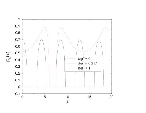
FIG. 1.: The dependence of the critical momentum $p_{c}=k_{c}/\mu$, Eq. (61), on time $\tau=t\,\mu$. A non-vanishing value indicates the appearance of tachyonic modes. The time dependence of $p_{c}$ is due to the alternating $\phi$-field and depends strongly on the choice of the initial values.

The total number of particles of all modes at any time $t$ is given by

$${\cal N}(t)=2\int_{0}^{\infty}\frac{d^{3}{\vec{k}}}{(2\pi)^{3}}{\cal N}_{+}(\vec{k},t).$$ (62)

Simple power counting yields that this expression is finite.

V Decay of the CP odd phase

In the vicinity of the phase transition the QCD vacuum rearranges: chiral symmetry breaking and confinement drive quark matter into hadronic states. In this region topological phenomena such as the appearance of a non-vanishing QCD $\theta$ angle may occur. As a consequence the CP symmetry is dynamically broken and in these regions a CP-odd phase can occur (paramater Set IV in Table I). In the rapid cooling of the hot QCD matter down to the critical temperature $T_{d}$, the U_A(1) breaking gets restored either completely (Set I) or partially (Sets II, III). After such a quench of the effective potential (63), the system is in the false vacuum state. The decay of this CP odd phase is a time dependent process and can be study within the kinetic approach introduced in the previous section.

The potential of the effective Lagrangian density (3)

$$V(\eta/f)\equiv-\cos\Big{(}\frac{\eta}{f}\Big{)}+\frac{a}{2\mu^{2}}(\eta/f)^{2}$$ (63)

is plotted in Fig. 2 for different values of the potential parameter, $a/{{\mu}^{2}}$, according to Table I.

FIG. 2.: The shape of the potential $V({\eta}/f)$, (63), is plotted for different values of $a/{{\mu}^{2}}$. Local minima characteristic for $a/{{\mu}^{2}}<1$ assumed at large temperatures disappear due to an applied fast quench.

Set	I	II	III	IV
$a/\mu^{2}\bigg{/}(a/\mu^{2})_{vac}$	1	1/2	1/4	0

TABLE I.: Different values of $a/\mu^{2}$ as used in the numerical calculation. ($a/\mu^{2})_{vac}\sim 4.24$ is the vacuum value for which all mesons have their vacuum masses. Set I assumes a fast quench after which the vacuum value is immediately reached, i.e. the $\eta^{\prime}$ mass assumes its vacuum value in the vicinity of $T_{d}$. This scenario is compared with slow quenches corresponding to parameters given in Set II and Set III. Set IV leads to the appearance of tachyonic modes; a value only possible for $T>T_{d}$.

Starting from the quark gluon plasma phase in which $a/{{\mu}^{2}}$ is suppressed, Set IV in Table I, the potential changes from the cosine shape to a parabolic shape due a sudden quench at the deconfinement phase transition. The metastable states located in the local minima of the potential roll smoothly back into the trivial minimum and oscillate around it. This situation is formalized in assumption (13): The ${\eta}$-field can be decomposed into its vacuum mean value ${\phi}(t)$ and its quantum fluctuations ${\chi}$. During the decay, energy is transferred from ${\phi}$ to ${\chi}$. As a result, ${\phi}$ is damped, while the number of particles in quantum fluctuations increases. It is assumed that during this process the temperature does not change essentially, and particle production proceeds in a fixed potential characterized by $a/{{\mu}^{2}}$. This process takes place on a time scale typical for the hadronisation process: $1-10$ fm/c.

FIG. 3.: The solution of the vacuum mean field equation as function of time, Eq. (B1), is shown for different values of $a/{{\mu}^{2}}$ (c.f. Table I) for the initial conditions $\phi(0)/f=2\pi$ and ${\dot{\phi}}(0)/f=0$. Note that for $a/\mu^{2}=0$, $\phi(\tau)$ would be constant.

The potential parameter $a/\mu^{2}$ depends on temperature due to medium dependent meson masses. However its exact behaviour near the critical temperature is unknown. Lattice calculations as well as QCD models suggest that $\pi$, $K$ and $\eta$ meson properties have only a weak dependence on $T$. About the response of $\eta^{\prime}$ to increasing $T$ is much less known and therefore we explore different scenarios summarised in Table I. Set I assumes that the medium dependence is negligible. Set II (III, IV) corresponds to an in-medium reduction of the $\eta^{\prime}$ mass of about 20 (40, 60)$\%$ applying the simple equations given in connection with Eq. (3), [23]. It is important to note that $f\sim f_{\pi}$ can be considered as an order parameter for the chiral phase transition and hence is strongly suppressed at $T_{d}$, i.e $f(T\sim T_{d})=0.1\,f(T=0)$. In the herein applied scenario, the in-medium dependent parameters $a/\mu^{2}$ and $f$ change only during the fast quench. Their time-dependence can therefore be neglected.

The solution of the non-linear Eq. (B1) for ${\phi}({\tau})$ with different $a/{{\mu}^{2}}$ is plotted in Fig. 3, employing the initial conditions ${\phi}(0)/f=2\pi$ and $(d{\phi}(\tau)/d{\tau})_{{\tau}=0}=0$ throughout the numerical calculations. We see that the period and the amplitude of the oscillations of ${\phi}({\tau})$ vary with the change of $a/{{\mu}^{2}}$. The oscillations are not damped since feedback of the fluctuations on the mean field is neglected. The field $\phi$ provides the background field for the solution of the quantum kinetic equation given in Eq. (B4).

VI Numerical results

The solution of the quantum kinetic equation (58) describes the production of $\eta^{\prime}$ particles: the momentum dependence and it’s time evolution. The strong back ground field, $\phi$, leading to a sizeable particle production rate is given by the solution of the non-linear Eq. (17), see Fig. 3.

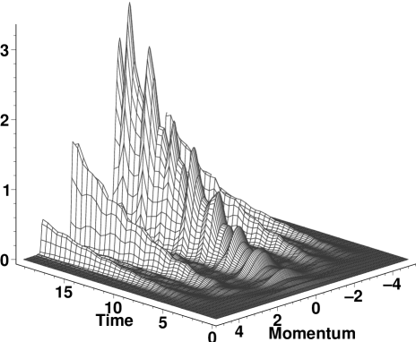
FIG. 4.: The time evolution of the momentum distribution function for parameter Set III. Most of the mesons are produced with small momenta but additional resonance bands appear for larger momenta; their maximal amplitude is smaller. The time evolution is characterized by an increase of the particle number and a repeated spike structure.

We perform the numerical calculation using dimensionless variables and solve the kinetic equation as a system of coupled differential equations, Eqs. (B10-B12), introduced in Appendix B. The decay starts at $\tau=0$, for which ${\cal N}_{+}(\vec{p},0)=0;\phi(0)=2\pi f$ and ${\dot{\phi}}(0)=0$ define the initial conditions.

As result we obtain the number of particles produced during the decay of the CP odd phase in the false vacuum. Herein we restricted ourselves to the study of the non-tachyonic regime, i.e. we explore the solution for positive frequencies, Eq. (B5), corresponding to $a/{{\mu}^{2}}>1$ given in Table I.

FIG. 5.: The time evolution of the particle number for two different $a/{{\mu}^{2}}>1$ when the system is in the non-tachyonic regime, (B4). The double spike structure on top of the rapid growth repeats periodically in tune with the mean field’s frequency (c.f. Fig. 3). An estimate in low density approximation shows that inclusion of the Bose quantum statistics leads to a pronounced enhancement.

In Fig. 4 we show the complete numerical solution. Two features are apparent: (i) the fast increase is characterised by a repeated structure on top of the curve, (ii) additional to the occupation of low momentum states we observe the appearance of resonance bands at larger momenta.

In Fig. 5 we plot the time evolution of the particle number for zero momentum and compare the solution for Set I and Set III. We observe a very fast increase of the number of produced particles. A maximum occupation of a given momentum state at a given time is reached for small values of the potential parameter, i.e. using Set III. For larger values of the potential parameter, e.g. Set I, less particles are produced in a given time since the source term is suppressed by a larger mass term $a/\mu^{2}$ in $\omega(p)$, see (B5).

The most striking feature in this plot is the periodically repeated spike structure on top of the overall growth, (c.f. [34]). This pattern appears with the same frequency as the background field oscillates, see Fig. 3. When back reactions are included this would possibly not be the case. The spike structure is smoother for Set I compared to Set III but still characteristic for the evolution.

Herein we also compare the full solution with the low density approximation (l.d.). The low density approximation assumes that ${\cal N}_{+}({\vec{p}},t)\ll 1$ and hence suggests that the solution of the kinetic equation does not depend on the pre-history of the systems evolution. Any calculation which does not retain quantum statistical effects necessarily employs this ansatz. From Fig. 5 it is plain that the inclusion of the Bose statistical factor into the kinetic equation leads to Bose enhancement as soon as $N_{+}\sim 1$, appearing at $\tau\sim 1$. This effect becomes more pronounced with increasing time.

FIG. 6.: The particle number as function of momentum, $p=|{\vec{p}}|$, for two different $a/{{\mu}^{2}}>1$. Bose enhancement of mainly the low momentum states is apparent. A characteristic second resonance band appears for large momenta.

The momentum dependence at a given time, Fig. 6, shows that most of the particles are produced with small momenta. Additional resonance bands appear. The smaller the value of the potential parameter is reached in the quench the closer the second maxima appears to the first one. The reason for this resonance effect is typical for the Mathieu type equation: the two intrinsic frequencies of the background field and of the production process are of the same order of magnitude and resonances are likely to appear.

In Fig. 6 we also compare the momentum dependence of the full non-Markovian solution with a calculation in low density limit. It is apparent that the Bose enhancement acts naturally on the lower momenta. For the considered case the occupation number is enhanced by a factor of 4. For large momenta details of the quantum statistics are suppressed. Therefore the higher resonance bands are much less affected by quantum corrections. It is plain from this study that quantum statistical effects cannot be neglected: the low density approximation is invalid if the produced number density exceeds a critical value at very early times of the evolution.

VII Summary

Starting from the singlet Witten-DiVecchia-Veneziano effective Lagrangian we have derived a quantum kinetic equation describing the production of ${\eta}^{\prime}$-mesons from a CP-odd metastable vacuum state. We have employed a general method based on the evolution operator holding also for other model langrangians. The vacuum mean field provides a classical, self-interacting strong background field. Quantum fluctuations around the dynamical mean field value are considered but their feedback to the background field is neglected. Due to these quantum fluctuations particles are produced and the time evolution of this process is described by a non-Markovian equation for the distribution function of the produced $\eta^{\prime}$ mesons.

We find that the details of the decay process depend strongly on the applied quench. The number of produced particles is much larger when the $\eta^{\prime}$ mass is suppressed in the vicinity of the phase boundary. Most of the particles are produced with low momenta, for large momenta additional resonances appear. Furthermore, we have demonstrated that quantum statistical effects are important and lead to a pronounced enhancement of the particle occupation number for low momenta. In the case $a/\mu^{2}<1$, tachyonic instabilities occur for momenta smaller than a critical value. This regime has not been considered herein.

The numerical investigation of the tachyonic modes and the inclusion of back reactions promise further insight into the decay of CP odd metastable states and its realization will be reported elsewhere.

A In-field quantization

The in-field is a solution of the equation

$$(\Box+m_{0}^{2}){\eta}_{in}=0.$$ (A1)

The in-field operators fulfill periodic boundary conditions and are expanded in Fourier modes

$${\eta}_{in}(\vec{x},t) = \frac{1}{\sqrt{V}}\sum_{\vec{k}}e^{i\vec{k}\vec{x}}{\eta}_{in}(\vec{k},t),$$ (A2)

$${\pi}_{in}(\vec{x},t) = \frac{1}{\sqrt{V}}\sum_{\vec{k}}e^{-i\vec{k}\vec{x}}{\pi}_{in}(\vec{k},t),$$ (A3)

where the summation is over discrete momenta $\vec{k}=\frac{2{\pi}}{L}\vec{n}$, $(n_{1},n_{2},n_{3})$ and

$${\eta}_{in}(\vec{k},t) = {\Gamma}_{\vec{k}}^{0}(t)a_{in}(\vec{k})+{\Gamma}_{\vec{k}}^{0,{\star}}(t)a_{in}^{\dagger}(-\vec{k}).$$ (A4)

$${\pi}_{in}(\vec{k},t) = \dot{\eta}_{in}^{\dagger}(\vec{k},t)$$ (A5)

$$= -i{\omega}_{k}^{0}\Big{[}{\Gamma}_{\vec{k}}^{0}(t)a_{in}(-\vec{k})-{\Gamma}_{\vec{k}}^{0,{\star}}(t)a_{in}^{\dagger}(\vec{k})\Big{]}.$$ (A6)

The time-independent creation and annihilation operators obey the commutation relations

$$[a_{in}(\vec{k}),a_{in}^{\dagger}(\vec{k}^{\prime})]_{-}=\delta_{\vec{k},\vec{k}^{\prime}},$$ (A7)

all other commutators vanish. The function ${\Gamma}_{\vec{k}}^{0}(t)$ is given by

$${\Gamma}_{\vec{k}}^{0}(t)=\frac{1}{\sqrt{2{\omega}_{k}^{0}}}\exp\{-i{\omega}_{k}^{0}t\}$$ (A8)

with ${\omega}_{k}^{0}\equiv\sqrt{\vec{k}^{2}+m_{0}^{2}}$. Since the field ${\eta}(\vec{x},t)$ is real, we have ${\eta}_{in}^{\dagger}(\vec{k},t)={\eta}_{in}(-\vec{k},t),$ and ${\pi}_{in}^{\dagger}(\vec{k},t)={\pi}_{in}(-\vec{k},t).$ The vacuum state $|0;in\rangle\equiv|0\rangle$ is defined as vanishing under the action of the annihilation operators $a_{in}(\vec{k})|0\rangle=0.$

B Numerical realization

The evolution of ${\phi}$ in the decay is governed by equation (17). Introducing the dimensionless vacuum mean field ${\phi}/f$ and the dimensionless time variable ${\tau}\equiv{\mu}t$, we rewrite (17) as

$$\frac{d^{2}}{d{\tau}^{2}}\Big{(}\frac{{\phi}(\tau)}{f}\Big{)}+\sin\Big{(}\frac{{\phi}(\tau)}{f}\Big{)}+\frac{a}{{\mu}^{2}}\Big{(}\frac{{\phi}(\tau)}{f}\Big{)}=0,$$ (B1)

with the one parameter $a/{{\mu}^{2}}$ characterizing the solution.

Note that for small $a/{{\mu}^{2}}\approx 0$ one can replace (B1) by the Sine- Gordon equation

$$\frac{d^{2}}{d{\tau}^{2}}\Big{(}\frac{{\phi}_{0}(\tau)}{f}\Big{)}+\sin\Big{(}\frac{{\phi}_{0}(\tau)}{f}\Big{)}=0,$$ (B2)

the subscript $(0)$ in ${\phi}(\tau)$ indicates the zero value of $a/{{\mu}^{2}}$. The solution of Eq. (B2) is a Jacobian elliptic function. Herein we do not make this approximation and solve (B1) numerically for nonzero values of $a/{{\mu}^{2}}$.

For the numerical study we introduce dimensionless variables for the kinetic equations and obtain

$$\frac{d}{d{\tau}}{\cal N}_{+}(\vec{p},{\tau})= \frac{\dot{\bar{\omega}}_{p}}{2\bar{\omega}_{p}}\int_{0}^{\tau}d{\tau}^{\prime}\frac{\dot{\bar{\omega}}_{p}}{\bar{\omega}_{p}}({\tau}^{\prime})\Big{(}1+2{\cal N}_{+}(\vec{p},{\tau}^{\prime})\Big{)}\times$$ (B4)

$$\cos[2{\Theta}_{p}^{ad}(\tau)-2{\Theta}_{p}^{ad}({\tau}^{\prime})]$$

where the dimensionless frequency is

$$\bar{\omega}_{p}^{2}\equiv\frac{1}{{\mu}^{2}}{\omega}_{k}^{2}={\vec{p}}^{~{}2}+\cos\Big{(}\frac{{\phi}(\tau)}{f}\Big{)}+\Big{(}\frac{a}{{\mu}^{2}}{\Big{)}}\,.$$ (B5)

with ${\vec{p}}^{~{}2}\equiv({\vec{k}^{2}}/{{\mu}^{2}})$.

Eq. (B4) is an integro-differential equation. It can be re-expressed by introducing

$$u(\vec{p},{\tau}) \equiv \int_{0}^{\tau}d{\tau}^{\prime}\frac{\dot{\bar{\omega}}_{p}}{\bar{\omega}_{p}}({\tau}^{\prime})\Big{(}1+2{\cal N}_{+}(\vec{p},{\tau}^{\prime})\Big{)}\times$$ (B7)

$$\sin[2{\Theta}_{p}^{ad}({\tau})-2{\Theta}_{p}^{ad}({\tau}^{\prime})],$$

$$v(\vec{p},{\tau}) \equiv \int_{0}^{\tau}d{\tau}^{\prime}\frac{\dot{\bar{\omega}}_{p}}{\bar{\omega}_{p}}({\tau}^{\prime})\Big{(}1+2{\cal N}_{+}(\vec{p},{\tau}^{\prime})\Big{)}\times$$ (B9)

$$\cos[2{\Theta}_{p}^{ad}({\tau})-2{\Theta}_{p}^{ad}({\tau}^{\prime})],$$

with the initial conditions $u(\vec{p},0)=v(\vec{p},0)=0$, in which case we have

$$\frac{d}{d{\tau}}{\cal N}_{+}(\vec{p},{\tau}) = \frac{\dot{\bar{\omega}}_{p}}{2\bar{\omega}_{p}}v(\vec{p},{\tau}),$$ (B10)

$$\frac{d}{d{\tau}}v(\vec{p},{\tau}) = \frac{\dot{\bar{\omega}}_{p}}{\bar{\omega}_{p}}\Big{(}1+2{\cal N}_{+}(\vec{p},{\tau})\Big{)}-2\bar{\omega}_{p}u(\vec{p},{\tau}),$$ (B11)

$$\frac{d}{d{\tau}}u(\vec{p},{\tau}) = 2\bar{\omega}_{p}v(\vec{p},{\tau}).$$ (B12)

REFERENCES

- [1] Proceedings: QUARK MATTER ’99: Proceedings. Edited by L. Riccati, M. Masera, E. Vercellin. Amsterdam, The Netherlands, North-Holland, 1999. (Nuclear Physics A, Vol. A661, December 1999).
- [2] F. Sauter, Z. Phys. 69 (1931) 742; W. Heisenberg and H. Euler, Z. Phys. 98 (1936) 714; J. Schwinger, Phys. Rev. 82 (1951) 664.
- [3] TESLA – The Superconductiong Electron Positron Linear Collider with an Integrated X-Ray Laser Laboratory, Technical Design Report, DESY 2001-011, ECFA 2001-209, TESLA-Report 2001-23, TESLA-FEL 2001-05;
- [4] A. Ringwald, Phys. Lett. B 510 (2001) 107; R. Alkofer, et al., nucl-th/0108046, Phys. Rev. Lett. in press.
- [5] T. Damour and R. Ruffini, Phys. Rev. D 14 (1976) 332.
- [6] L. Parker, Phys. Rev. 183 (1969) 1057.
- [7] A. Casher, H. Neuberger and S. Nussinov, Phys. Rev. D 20 (1979) 179; B. Andersson, G. Gustafson, G. Ingelman and T. Sjöstrand, Phys. Rept. 97 (1983) 31; T. S. Biro, H. B. Nielsen and J. Knoll, Nucl. Phys. B 245 (1984) 449.
- [8] S.A. Smolyansky et al., hep-ph-9712377; S.M. Schmidt et al., Int. J.Mod. Phys. E 7 (1998) 709; Y. Kluger, E. Mottola, and J.M. Eisenberg, Phys. Rev. D 58 (1998) 125015.
- [9] J. Rau and B. Müller, Phys. Rep. 272 (1996) 1.
- [10] S.M. Schmidt et al., Phys. Rev. D 59 (1999) 094005; S. M. Schmidt, A. V. Prozorkevich and S. A. Smolyansky, hep-ph/9809233; J.C.R. Bloch, C.D. Roberts, and S.M. Schmidt, Phys. Rev. D 61 (2000) 117502.
- [11] K. Kajantie and T. Matsui, Phys. Lett. B 146 (1985) 373; G. Gatoff, A.K. Kerman and T. Matsui, Phys. Rev. D 36 (1987) 114.
- [12] J.M. Eisenberg and G. Kälbermann, Phys. Rev. D 37 (1988) 1197; Y. Kluger et al., Phys. Rev. Lett. 67 (1991) 2427; Phys. Rev. D 45 (1992) 4659; F. Cooper et al., Phys. Rev. D 48 (1993) 190;
- [13] R.S. Bhalerao and G.C. Nayak, Phys. Rev. C 61 (2000) 054907;Q. Wang, C. Kao, G. C. Nayak, H. Stoecker and W. Greiner, hep-th/0009076; K. Bajan and W. Florkowski, hep-ph/0107244.
- [14] J. Bloch et al., Phys. Rev. D 60 (1999) 116011, A.V. Prozorkevich et al., nucl-th/0012039; D.V. Vinnik et al., nucl-th/0103073, Eur. Phys. J. C in press.
- [15] C.D. Roberts and S.M. Schmidt, Prog. Part. Nucl. Phys. 45 (2000) S1.
- [16] E. Laermann, Phys. Part. Nucl. 30 (1999) 304 [Fiz. Elem. Chast. Atom. Yadra 30 (1999) 720].
- [17] R. Alkofer and L. von Smekal, Phys. Rept. 353 (2001) 281.
- [18] ECT* International Workshop on Understanding Deconfinement in QCD, Trento, Italy, 1-13 Mar 1999. UNDERSTANDING DECONFINEMENT IN QCD: Proceedings. Edited by David Blaschke, Frithjof Karsch, Craig D. Roberts. World Scientific, 2000.
- [19] S. P. Klevansky, Rev. Mod. Phys. 64 (1992) 649.
- [20] A. Bender et al., Phys. Rev. Lett. 77 (1996) 3724; C. D. Roberts, Phys. Part. Nucl. 30 (1999) 223 [Fiz. Elem. Chast. Atom. Yadra 30 (1999) 537].
- [21] D. Kharzeev, R.D. Pisarski, and M.H.C. Tytgat, Phys. Rev. Lett. 81 (1998) 512; D. Kharzeev and R.D. Pisarski, Phys. Rev. D 61 (2000) 111901; D. Kharzeev, A. Krasnitz, and R. Venugopalan, hep-ph/0109253.
- [22] J. Kapusta, D. Kharzeev, and L. McLerran, Phys. Rev. D 53 (1996) 5028; Z. Huang and X.-N. Wang, Phys. Rev. D 53 (1996) 5034.
- [23] R. Alkofer, P. A. Amundsen and H. Reinhardt, Phys. Lett. B 218 (1989) 75.
- [24] D. Ahrensmeier, R. Baier, and M. Dirks, Phys. Lett. B 484 (2000) 58.
- [25] G. Veneziano, Nucl. Phys. B 159 (1979) 213; P. Di Vecchia and G. Veneziano, Nucl. Phys. B 171 (1980) 253; P. Di Vecchia et al., Nucl. Phys. B 181 (1981) 318; E. Witten, Nucl. Phys. B 156 (1979) 269; Annals Phys. 128 (1980) 363; Phys. Rev. Lett. 81 (1998) 2862.
- [26] H. Reinhardt and R. Alkofer, Phys. Lett. B 207 (1988) 482;
- [27] R. Alkofer and I. Zahed, Phys. Lett. B 238 (1990) 149.
- [28] P. Maris, C. D. Roberts and S. M. Schmidt, Phys. Rev. C 57 (1998) 2821; P. Maris et al., Phys. Rev. C 63 (2001) 025202; D. Blaschke et al., Int. J. Mod. Phys. A 16 (2001) 2267.
- [29] L. Landau and E. Lifshitz, Mechanics (Pergamon, Oxford, 1960); V. Arnold, Mathematical Methods of Classical Mechanics (Springer, New York, 1978).
- [30] J. Traschen and R. Brandenberger, Phys. Rev. D 42 (1990) 2491; R.H. Brandenberger, hep-ph-0102183.
- [31] D.A. Kirzhnits and A.D. Linde, Phys. Lett. B 42 (1972) 471; Ann. Phys. (NY) 101 (1976) 195; S. Weinberg, Phys. Rev. D 9 (1974) 3357; L. Dolan and R. Jackiw, Phys. Rev. D 9 (1974) 3320.
- [32] A.A. Anselm and M.G. Ryskin, Phys. Lett. B 266 (1991) 482; K. Rajagopal and F. Wilczek, Nucl. Phys. B 399 (1993) 395; B 404 (1993) 577; D. Boyanovsky, H.J. de Vega, and R. Holman, Phys. Rev. D 51 (1995) 734.
- [33] G. Felder et al., Phys. Rev. Lett. 87 (2001) 011601.
- [34] G. Felder, L. Kofman, and A. Linde, hep-th-0106179.