Parity-Violating Interaction Effects I: the Longitudinal Asymmetry in Elastic Scattering
Abstract
The proton-proton parity-violating longitudinal asymmetry is calculated in the lab-energy range 0–350 MeV, using a number of different, latest-generation strong-interaction potentials–Argonne , Bonn-2000, and Nijmegen-I–in combination with a weak-interaction potential consisting of - and -meson exchanges–the model known as DDH. The complete scattering problem in the presence of parity-conserving, including Coulomb, and parity-violating potentials is solved in both configuration- and momentum-space. The predicted parity-violating asymmetries are found to be only weakly dependent upon the input strong-interaction potential adopted in the calculation. Values for the - and -meson weak coupling constants and are determined by reproducing the measured asymmetries at 13.6 MeV, 45 MeV, and 221 MeV.
pacs:
21.30.+y, 24.80.-x, 25.40.CmI Introduction
A new generation of experiments have recently been completed, or are presently under way or in their planning phase to study the effects of parity-violating (PV) interactions in elastic scattering [1], radiative capture [2] and deuteron electro-disintegration [3] at low energies. There is also considerable interest in determining the extent to which PV interactions can affect the longitudinal asymmetry measured by the SAMPLE collaboration in quasi-elastic scattering of polarized electrons off the deuteron [4], and therefore influence the extraction from these data (and those on the proton [5]) of the nucleon’s strange magnetic and axial form factors at a four-momentum transfer squared of (GeV/c)2.
The present is the first in a series of papers dealing with the theoretical investigation of PV interaction effects in two-nucleon systems: it is devoted to elastic scattering, and presents a calculation of the longitudinal asymmetry induced by PV interactions in the lab-energy range 0–350 MeV.
The available experimental data on the longitudinal asymmetry is rather limited. There are two measurements at 15 MeV [6] and 45 MeV [7], which yielded asymmetry values of and , respectively, as well as more precise measurements at 13.6 MeV [8], 45 MeV [9], and 221 MeV [1] yielding , , and , respectively, and finally a measurement at 800 MeV in Ref. [10], which produced an asymmetry value of .
The theoretical (and, in fact, experimental) investigation of PV effects induced by the weak interaction in the system began with the prediction by Simonius [11] that the longitudinal asymmetry would have a broad maximum at energies close to 50 MeV, and that, being dominated by the =0 partial waves, it would be essentially independent of the scattering angle. A number of theoretical studies of varying sophistication followed [12, 13, 14], culminating in the study by Driscoll and Miller [15], who used a distorted-wave Born-approximation (DWBA) formulation of the PV scattering amplitude in terms of exact wave functions obtained from solutions of the Schrödinger equation with Coulomb and strong interactions. In fact, the authors of Ref. [15] investigated the sensitivity of the calculated asymmetry to a number of realistic strong-interaction potentials constructed by the late 1980’s. The model adopted for the PV weak-interaction potential, however, was that developed by Desplanques and collaborators [16], the so-called DDH model. In the sector, this potential is parametrized in terms of - and -meson exchanges, in which the PV and weak coupling constants are calculated in a quark model approach incorporating symmetry techniques like SU(6)W and current algebra requirements. Factoring in the limitations inherent to such an approach, however, the authors of Ref. [16] gave rather wide ranges of uncertainty for these weak coupling constants.
The present work sharpens and updates that of Ref. [15]. It adopts the DDH model for the PV weak-interaction potential, but uses the latest generation of realistic, parity-conserving (PC) strong-interaction potentials, the Argonne [17], Nijmegen I [18], and CD-Bonn [19]. Rather than employing the DWBA scheme of Ref. [15] to calculate the PV component of the elastic scattering amplitude, it solves the complete scattering problem in the presence of these PC and PV potentials (including the Coulomb potential), in either configuration- or momentum-space, depending on whether the Argonne and Nijmegen I or CD-Bonn models are used. Such an approach allows us to obtain the PC and PV wave functions explicitly. While this is unnecessary for the calculation reported here–the DWBA estimate, along the lines of Ref. [15], of the PV component of the amplitude should suffice–it becomes essential for the studies of radiative capture and deuteron electro-disintegration planned at a later stage.
The remainder of the present paper is organized as follows. In Sec. II the PC and PV potentials used in this work are briefly described, while in Sec. III a self-consistent treatment of the scattering problem is provided along with a discussion, patterned after that of Ref. [15], of the Coulomb contributions to the longitudinal asymmetries measured in scattering and transmission experiments. In Sec. IV the results for the asymmetry are presented; in particular, their sentitivity to changes in the values of the weak coupling constants and/or short-range cutoffs at the strong- and weak-interaction vertices is studied. Finally, Sec. V contains some concluding remarks.
II Parity-Conserving and Parity-Violating Potentials
The parity-conserving (PC), strong-interaction potentials used in the present work are the Argonne (AV18) [17], Nijmegen I (NIJ-I) [18], and CD-Bonn (BONN) [19] models. The AV18 and NIJ-I potentials were fitted to the Nijmegen database of 1992 [20, 21], consisting of 1787 data, and both produced per datum close to one. The latest version of the charge-dependent Bonn potential, however, has been fit to the 1999 database, consisting of 2932 data, for which it gives a per datum of 1.01 [19]. The substantial increase in the number of data is due to the development of novel experimental techniques–internally polarized gas targets and stored, cooled beams. Indeed, using this technology, IUCF has produced a large number of spin-correlation parameters of very high precision, see for example Ref. [22]. It is worth noting that the AV18 potential, as an example, fits the post-1992 and both pre- and post-1992 data with ’s of 1.74 and 1.35, respectively [19]. Therefore, while the quality of their fits has deteriorated somewhat in regard to the extended 1999-database, the AV18 and NIJ-I models can still be considered “realistic”.
These realistic potentials consist of a long-range part due to one-pion exchange (OPE), and a short-range part either modeled by one-boson exchange (OBE), as in the BONN and NIJ-I models, or parameterized in terms of suitable functions of two-pion range or shorter, as in the AV18 model. While these potentials are (almost) phase-equivalent, they differ in the treatment of non-localities. AV18 is local (in channels), while BONN and NIJ-I have strong non-localities. In particular, BONN has a non-local OPE component. However, it has been known for some time [23], and recently re-emphasized in Ref. [24], that the local and non-local OPE terms are related to each other by a unitary transformation. Therefore, the differences between local and non-local OPE cannot be of any consequence for the prediction of observables, such as binding energies or electromagnetic form factors, provided, of course, that three-body interactions and/or two-body currents generated by the unitary transformation are also included [25]. This fact has been demonstrated [26] in a calculation of the deuteron structure function and tensor observable , based on the local AV18 and non-local BONN models and associated (unitarily consistent) electromagnetic currents. The remaining small differences between the calculated and are due to the additional short-range non-localities present in the BONN model. Therefore, provided that consistent calculations–in the sense above–are performed, present “realistic”potentials will lead to very similar predictions for nuclear observables, at least to the extent that these are influenced predominantly by the OPE component.
As already mentioned in Sec. I, the form of the parity-violating (PV) weak-interaction potential was derived in Ref. [16]–the DDH model:
| (1) | |||||
| (2) |
where the relative position and momentum are defined as and , respectively, denotes the anticommutator, and and are the proton and vector-meson ( or ) masses, respectively. Note that the first term in Eq. (2) is usually written in the form of a commutator, since
| (3) |
where denotes its derivative . The Yukawa function , suitably modified by the inclusion of monopole form factors, is given by
| (4) |
where . Finally, the values for the strong-interaction - and -meson vector and tensor coupling constants and , as well as for the cutoff parameters , are taken from the BONN model [19], and are listed in Table I. The weak-interaction coupling constants and correspond to the following combinations of DDH parameters
| (5) | |||||
| (6) |
Their values, reported in Table I in the column labeled (DDH-adj), are obtained by fitting the available data on the longitudinal asymmetry, see Sec. IV. The values corresponding to the “best”estimates for the and suggested in Ref. [16] are also listed in Table I in the column (DDH-orig). Indeed, one of the goals of the present work is to study the sensitivity of the calculated longitudinal asymmetry to variations in both the PV coupling constants and cutoff parameters. In this respect, it should also be noted that, in the limit = and ignoring the small mass difference between and , were it not for the different values of the tensor couplings and , the - and -meson terms in would collapse to a single term of strength proportional to .
III Formalism
In this section we discuss the scattering problem in the presence of a potential given by
| (7) |
where and denote the parity-conserving and parity-violating components induced by the strong and weak interactions, respectively, and is the Coulomb potential.
A Partial-Wave Expansions of Scattering State, - and -Matrices
The Lippmann-Schwinger equation for the scattering state , where is the relative momentum and specifies the spin state, can be written as [27]
| (8) |
where is the free Hamiltonian, , and are the eigenstates of ,
| (9) |
with wave functions given by
| (10) | |||||
| (11) |
Here denotes the regular Coulomb wave function [28], while the parameter and Coulomb phase-shift are given by
| (12) | |||||
| (13) |
where is the fine structure constant and is the reduced mass. Finally, the following definitions have also been introduced:
| (14) |
| (15) |
The factor ensures that the wave functions are properly antisymmetrized. Note that in the limit =0, equivalent to ignoring the Coulomb potential, the latter reduce to (antisymmetrized) plane waves,
| (16) |
The -matrix corresponding to the potential can be expressed as [27]
| (17) |
where is the (known) -matrix corresponding only to the Coulomb potential [27], and
| (18) |
Insertion of the complete set of states into the right-hand-side of the Lippmann-Schwinger equation leads to
| (19) |
from which the partial wave expansion of the scattering state is easily obtained by first noting that the potential, and hence the -matrix, can be expanded as
| (21) | |||||
with
| (22) |
After insertion of the corresponding expansion for the -matrix into Eq. (19) and a number of standard manipulations, the scattering-state wave function can be written as
| (23) |
with
| (24) | |||||
| (25) |
The (complex) radial wave function behaves in the asymptotic region as
| (26) |
where the label () stands for the set of quantum numbers (), the on-shell () -matrix has been introduced,
| (27) |
and the functions are defined in terms of the regular and irregular () Coulomb functions as
| (28) |
Again, in the limit , and , where and are the spherical Bessel functions, and the familiar expressions for the partial wave-expansion of the scattering state, - and -matrices are recovered [27].
B Schrödinger Equation, Phase-Shifts, and Mixing Angles
The coupled-channel Schrödinger equations for the radial wave functions read:
| (29) |
with
| (30) |
where, because of time reversal invariance, the matrix can be shown to be real and symmetric (this is the reason for the somewhat unconventional phase factor in Eq. (30); in order to mantain symmetry for both the - and -matrices, and hence the -matrix, the states used here differ by a factor from those usually used in nucleon-nucleon scattering analyses). The asymptotic behavior of the ’s is given in Eq. (26).
The Pauli principle requires that there be a single channel when is odd, and three coupled channels when is even, with the exception of =0 in which case there are only two coupled channels, 1S0 and 3P0. The situation is summarized in Table II. Again because of the invariance under time-inversion transformations of , the -matrix is symmetric (apart from also being unitary), and can therefore be written, for the coupled channels having even, as [27]
| (31) |
where is a real orthogonal matrix, and is a diagonal matrix of the form
| (32) |
Here is the (real) phase-shift in channel , which is function of the energy . The mixing matrix can be written as
| (33) | |||||
| (34) |
where is the or orthogonal matrix, that includes the coupling between channels and only, for example
Thus, for =0 there are two phase-shifts and a mixing angle, while for even there are three phases and three mixing angles. Of course, since , the mixing angles induced by are , a fact already exploited in the last expression above for . Given the channel ordering in Table II, Table III specifies which of the channel mixings are induced by and which by .
The reality of the potential matrix elements makes it possible to construct real solutions of the Schrödinger equation (29). The problem is reduced to determining the relation between these solutions and the complex ’s functions. Using Eq. (31) and , the ’s can be expressed in the asymptotic region as
| (35) | |||||
| (36) |
where the has been dropped for simplicity. The expression above is real apart from the . To eliminate this factor, the following linear combinations of the ’s are introduced
| (37) | |||||
| (38) |
and the ’s are then the sought real solutions of Eq. (29).
The asymptotic behavior of the ’s can now be read off from Eq. (38) once the -matrices above have been constructed. The latter can be written as, up to linear terms in the “small”mixing angles induced by ,
Inverting the first line of Eq. (38),
| (39) |
and inserting the resulting expressions into Eq. (29) leads to the (in general, coupled-channel) Schrödinger equations satisfied by the (real) functions . They are identical to those of Eq. (29), but for the ’s being replaced by the ’s. These equations are then solved by standard numerical techniques. Note that: i) , since the diagonal matrix elements of vanish because of parity selection rules; ii) in the coupled equations with even, terms of the type involving the product of a parity-violating potential matrix element with a -induced wave function are neglected.
C Amplitudes, Cross Sections, and the Parity-Violating Asymmetry
The amplitude for elastic scattering from an initial state with spin projections , to a final state with spin projections , is given by
| (41) | |||||
where the amplitude is related to the -matrix defined in Eq. (17) via
| (42) |
Note that the direction of the initial momentum has been taken to define the spin quantization axis (the -axis), is the angle between and , the direction of the final momentum, and the energy (). The amplitude is split into two terms, , as in Eq. (17). Using the expansion of the -matrix, Eq. (21) with replaced by , and the relation between the - and -matrices, Eq. (27), the amplitude induced by can be expressed as
| (44) | |||||
while the partial-wave expansion of the amplitude associated with the Coulomb potential reads [27]:
| (45) |
The differential cross section for scattering of a proton with initial polarization is then given by
| (46) |
and the longitudinal asymmetry is defined as
| (47) |
where denote the initial polarizations . Carrying out the spin sums leads to the following expression for the asymmetry:
| (48) |
from which it is clear that the numerator would vanish in the absence of parity-violating interactions, since , in contrast to , cannot change the total spin of the pair.
Parity-violating scattering experiments typically measure the asymmetry weighted over a range of scattering angles,
| (49) |
where is the spin-averaged differential cross section. In contrast, transmission experiments measure the transmission of a polarized proton beam through a target. A cross section is then inferred from the transmission measurement. Beam particles elastically scattered by angles greater than some small critical angle are removed from the beam, thus reducing the observed transmission and adding to the inferred cross section. Beam particles scattered at angles smaller than are not distinguished from the beam and do not contribute to the cross section. To derive an expression for the asymmetry in this case, one needs to carefully consider the Coulomb contribution to the cross section–a divergent quantity in the limit . To this end, following Ref. [29], one first defines the differential cross sections
| (50) | |||||
| (51) |
and
| (52) |
and hence
| (53) |
In transmission experiments, the quantity of interest is
| (54) | |||||
| (55) |
where is explicitly given by
| (56) |
To evaluate , one writes, following Ref. [29]:
| (57) | |||||
| (58) |
Application of the optical theorem to the total cross sections and allows one to deduce
| (59) |
and the determination of the cross section is reduced to evaluating the integral on the right-hand-side of Eq. (58). For sufficiently small and by appropriately taking the limit in the integral of the interference term , which essentially entails taking the limit term by term in the partial-wave expansion of , one finds
| (60) |
neglecting terms of order and higher. Using Eqs. (56) and (60), the longitudinal asymmetry measured in transmission experiments is obtained as
| (61) |
with .
D Momentum-Space Formulation
In order to consider the (parity-conserving) Bonn potential [19], it is necessary to develop techniques to treat the scattering problem in momentum space. A method first proposed in Ref. [30] and most recently applied in Ref. [19] is used here. It consists in separating the potential into short- and long-range parts and , respectively,
| (62) |
where
| (63) | |||||
| (64) |
and is the Heaviside step function, =1 if , =0 otherwise. The radius is chosen large enough, so that vanishes for (in the present work, fm).
Since is of finite range, standard momentum-space techniques can now be used to solve for the -matrix in the channel(s):
| (65) | |||||
| (66) |
where denotes a principal-value integration, and the momentum-space matrix elements of the potential are defined as in Eq. (30), but for the replacements and . Note that performing the Bessel transforms of a Coulomb potential truncated at poses no numerical problem. The integral equations (66) are discretized, and the resulting systems of linear equations are solved by direct numerical inversion. The principal-value integration is eliminated by a standard subtraction technique [31].
The asymptotic wave functions associated with have the form:
| (67) |
where
| (68) |
and being the regular and irregular spherical Bessel functions, respectively, and the constants can only depend upon the entrance channel , see the Schrödinger equations (29). These wave functions should match smoothly, at =, those associated with the full potential , which behave asymptotically as in Eq. (26). Carrying out the matching for the functions and their first derivatives leads to a relation between the -matrices and , corresponding to and , respectively. In terms of -matrices, related to the corresponding -matrices via
| (69) |
and similarly and , this relation reads in matrix notation [32]:
| (70) | |||||
| (71) |
where the dependence upon is understood, and the diagonal matrices and have been defined as
| (72) | |||||
| (73) |
with the functions
E Matrix elements of in channel
To evaluate the radial functions of the PV potential in Eq. (30)–those associated with the PC potential are well known–one needs the matrix elements of and between spin-angle functions. Using the notation
| (75) |
and writing
| (76) |
where the symbol indicates that the partial derivatives must act to the right, one finds that the non-vanishing matrix elements are:
| (77) | |||||
| (78) |
IV Results and Discussion
In this section we present results for the longitudinal asymmetry in the lab energy range 0–350 MeV. The calculations use any of the modern strong-interaction potentials, either Argonne (AV18) [17], or CD-Bonn (BONN) [19], or Nijmegen-I (NIJ-I) [18], in combination with the DDH weak-interaction potential parameterized in terms of - and -meson exchanges [16]. The values for the - and -meson coupling constants and cutoff parameters are listed in Table I. The strong-interaction coupling constants and cutoff parameters are taken from the BONN potential, while the weak-interaction coupling constants and have been determined by an AV18-based fit to the observed asymmetry. In Table I we also list the and values corresponding to the “best”estimates for the and suggested in Ref. [16], column labeled DDH-orig.
The data points for the longitudinal asymmetry at 13.6 MeV, 45 MeV, and 221 MeV are those reported in Ref. [1, 33], and their values are , , and , respectively. The first point at 13.6 MeV has been obtained [33] by taking the weighted mean–and accounting for the square-root energy dependence–of the latest result from the the Bonn experiment at 13.6 MeV, as reported by Eversheim (Ref. [14] in Ref. [1]), and the 15 MeV result from Ref. [6]. The point at 45 MeV has also been obtained [33] by combining results from measurements at 45 MeV [9], 46 MeV, and 47 MeV (these last two both from Ref. [33]). The last point at 221 MeV is that reported in Ref. [1]. Finally, the errors include both statistical and systematic errors added in quadrature.
The total longitudinal asymmetry, shown in Fig. 1 for a number of combinations of strong- and weak-interaction potentials, is defined as
| (81) |
where the amplitudes are those given in Eq. (44). The expression above for ignores the contribution of the Coulomb amplitude, Eq. (45), divergent in the limit =0, and for this reason will be referred to as the “nuclear”asymmetry. Of course, one should note that Coulomb potential effects enter into explicitly through the Coulomb phase shifts, present in the partial-wave expansion for , and implicitly through the wave functions, from which the -matrix elements are calculated. The effect of including explicitly the amplitude induced by the Coulomb potential is discussed below.
The calculated nuclear asymmetries in Fig. 1 were obtained by retaining in the partial-wave expansion for all channels with up to . The curves labeled AV18, BONN, and NIJ-I all use the DDH potential with the coupling constants and determined by a rough fit to data (the AV18 is used in the fitting procedure). There is very little sensitivity to the input strong-interaction potential, certainly much less than one would infer from Fig. 1 of Ref. [15]. This is undoubtedly a consequence of the more extended and scattering data-base to which present potentials are fitted, as well as of the much higher accuracy achieved in these fits. An analysis of the extracted and coupling constants and their errors is presented later in this section.
We also show in Fig. 1 the AV18 results which correspond to a DDH potential using the “best”estimates for the and coupling constants [16] (values in column DDH-orig in Table I), with the remaining - and -meson strong-interaction coupling constants and cutoff parameters as given in Table I. A number of comments are now in order. The data point at 221 MeV essentially determines the value of . As pointed out by Simonius [34] (see also below), the dominant contributions to the total asymmetry in the energy range under consideration here are those associated with the 1S0-3P0 and 3P2-1D2 partial waves. At energies close to 225 MeV the 1S0-3P0 contribution, which can easily be shown to be proportional to using Eq. (44) (here and are the strong-interaction phases), vanishes. As a result, the total asymmetry in this energy region is almost entirely due to the 3P2-1D2 contribution, which is known [34] to be approximately proportional to the following combination of coupling constants, . In the BONN model, the -meson tensor coupling constant is taken to be zero, and hence the data point at 221 MeV fixes (for given , , and ). This is the reason for the % increase (in magnitude) of with respect to the DDH “best”estimate.
Below 50 MeV, however, the calculated total asymmetry is dominated by the 1S0-3P0 contribution, approximately proportional to [34] . The increase in magnitude of required to fit the point at 221 MeV, now leads to a total asymmetry below 50 MeV, which is too large when compared to experiment. Thus, in order to reproduce the 13.6 MeV and 45 MeV data points, the overall strength of the coupling constant combination above needs to be reduced significantly. Since and have the same sign, this requires making the sign of opposite to that of .
It is worth pointing out, though, that the changes in value for and advocated here are still compatible with the “reasonable”ranges for the and , determined in Ref. [16].
Finally, we show in Fig. 1 the total nuclear asymmetry obtained in a calculation based on the old Reid soft-core potential [35, 36] and a DDH potential using the following coupling-constant and cutoff values: , , , , GeV/c, GeV/c (these are all from the old -space version of the Bonn potential [37]), and the “best”estimates for and . These model interactions are essentially identical to those employed by Driscoll and Miller in Ref. [15]. Indeed, our calculated total asymmetry is close to that obtained by these authors. It should be stressed that in Ref. [15] the strong-interaction phases and mixing angles were taken from Arndt’s analysis of nucleon-nucleon scattering data [38] rather than calculated from the Reid soft-core potential, as done here. This is presumably the origin of the remaining small differences between their results and ours.
Figure 2 shows the total nuclear asymmetries obtained by including only the =0 channel (1S0-3P0) and, in addition, the =2 channels (3P2-1D2 and 3F2-1D2), and finally all (even) -channels up to =8. We re-emphasize that in the energy range 0–350 MeV the asymmetry is dominated by the 0 and 2 contributions (among the latter, specifically those from the 3P2-1D2 partial waves).
Figure 3 illustrates the sensitivity of the total nuclear asymmetry to modifications of the and cutoff parameters in the DDH potential. Both cot-offs are multiplied by , in each case and are then readjusted to approximately reproduce the AV18+DDH-adj combination. In the near point-like limit (=10), the asymmetry increases in magnitude by roughly a factor of 2 prior to adjustment. The resulting couplings used for this case are =–14.33 and =+3.95. Results are also shown for =1.5 and 0.8, the latter is an extreme case where the cutoff parameters are near the meson masses used to determine the ranges. Nevertheless, the energy dependence of the asymmetry is in all cases very similar. The couplings used to generate the two other curves are: for =1.5, =–15.32 and =+3.92; and for =0.8, =–106.7 and =+14.63.
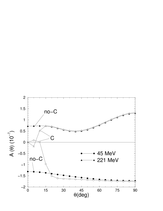
Figures 4–6 illustrate the effects of Coulomb contributions on the longitudinal asymmetry. Figure 4 compares the total nuclear asymmetry defined above (curve labeled “C”) with the total asymmetry obtained by ignoring the Coulomb potential altogether (curve labeled “no-C”). As already pointed out in Ref. [15], Coulomb contributions to these (non-physical) quantities are rather small.
Figure 5 compares the angular distribution of the (physical) longitudinal asymmetry obtained from the amplitudes , see Eq. (48), with that calculated by replacing in Eq.(48), namely ignoring the contribution of the Coulomb amplitude . The latter dominates at small scattering angles, and leads to the peculiar small angle behavior of the angular distribution shown in Fig. 5, namely its changing of sign at small , and its vanishing at =0 (also observed in Ref. [15]). It is interesting to note that the angular distribution at 230 MeV obtained by the authors of Ref. [15] is significantly different from that shown in Fig. 5 at 221 MeV.
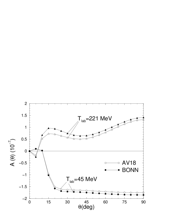
Figure 6 illustrates the effects of Coulomb contributions on the total longitudinal asymmetry measured in transmission experiments, Eq. (61), for various choices of the critical angle (=2∘, 5∘, and 10∘), see Eq. (55). Coulomb contributions are substantial, particularly for small and energies below 100 MeV. We also demonstrate, in Fig. 7, that the angular distributions of the longitudinal asymmetry are only weakly affected by different input (strong-interaction) potentials.
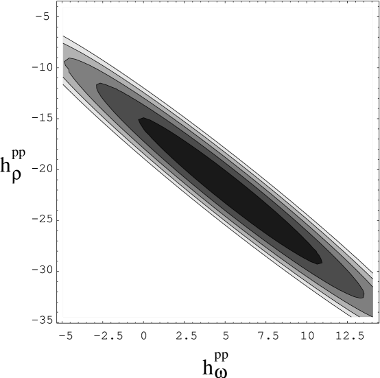
Finally, we present an analysis of the extracted coupling constants and their experimental errors. This analysis employs the AV18 model and the BONN-derived strong interaction couplings and cut-offs (Table I) in the DDH potential. Given the weak sensitivity described earlier, only small changes should be expected with the use of other recent strong interaction potentials. The experimental data at low energies have been combined into the two data points shown in Fig. 1 at 13.6 and 45 MeV. The asymmetries are –0.97 0.2 and –1.53 0.21, respectively, combining statistical and systematic errors. We also include the recent TRIUMF result of +0.84 0.34 at 221 MeV (all in units of ).
Figure 8 shows contours of constant total at levels of 1 through 5 versus the coupling constants and . As is apparent in the figure, there is a rather narrow band of acceptable values for and at total for the 3 experimental data points. At this level, can range from approximately –14 to –28, with a simultaneous (and strongly-correlated) variation in from rougly –2 to +10, all in units of .
V Conclusions
We have performed an analysis of the parity-violating (PV) longitudinal asymmetry using combinations of modern-day strong interaction potentials and the DDH PV potential. The new experimental results from TRIUMF at 221 MeV, in combination with previous results at lower energy, provide a strong constraint on allowable linear combinations of and PV coupling constants. Combining the statistical and systematic errors in quadrature, is constrained by present data to approximately 35%, at the level of one standard deviation.
The prime motivation for the present work is to initiate a systematic and consistent study of many PV observables in the few-nucleon sector, where accurate microscopic calculations are feasible. Recent measurements of nuclear anapole moments in atomic PV experiments are difficult to reconcile with earlier PV experiments in light nuclei using the simple DDH-orig model [39]. Up to now, this approach has been extremely limited by the available data.
The present experimental data in the few-nucleon sector remain rather sparse, with primary constraints coming from the longitudinal asymmetry analyzed here and measurements of the PV asymmetry in elastic scattering [40]. A variety of new results are expected in the next few years, however, including [2], the neutron spin rotation in Helium [41], and electron scattering measurements at Bates and JLAB. The combination of these diverse experiments should finally yield a coherent picture of the NN PV interaction at the hadronic scale.
Acknowledgments
We wish to thank R. Machleidt for providing us with computer codes generating the latest version of the Bonn potential, and for illuminating correspondence in regard to the treatment of the Coulomb potential in momentum space. The work of J.C. and B.F.G. was supported by the U.S. Department of Energy under contract W-7405-ENG-36, and the work of R.S. was supported by DOE contract DE-AC05-84ER40150 under which the Southeastern Universities Research Association (SURA) operates the Thomas Jefferson National Accelerator Facility. Finally, some of the calculations were made possible by grants of computing time from the National Energy Research Supercomputer Center.
REFERENCES
- [1] A.R. Berdoz et al., nucl-ex/0107014, submitted to Phys. Rev. Lett. (2001).
- [2] W. M. Snow, et al., Nucl. Instrum. Meth. A440, 729 (2000).
- [3] B. Wojtsekhowski and W.T.H. van Oers (spokespersons), JLAB letter-of-intent 00-002.
- [4] R. Hasty et al., Science 290, 2021 (2000).
- [5] D.T. Spayde et al., Phys. Rev. Lett. 84, 1106 (2000).
- [6] D.E. Nagle et al., in High Energy Physics with Polarized Beams and Polarized Targets–1978, edited by G.H. Thomas, AIP Conference Proceedings No. 51 (American Institute of Physics, New York, 1979), p. 218.
- [7] R. Balzer et al., Phys. Rev. C 30, 1409 (1984).
- [8] P.D. Eversheim et al., Phys. Lett. B 256, 11 (1991).
- [9] S. Kistryn et al., Phys. Rev. Lett. 58, 1616 (1987).
- [10] V. Yuan et al., Phys. Rev. Lett. 57, 1680 (19886).
- [11] M. Simonius, Phys. Lett. 41B, 415 (1972).
- [12] V.R. Brown, E.M. Henley, and F.R. Krejs, Phys. Rev. C 9, 935 (1973); Phys. Rev. Lett. 30, 770 (1973).
- [13] E.M. Henley and F.R. Krejs, Phys. Rev. D 11, 605 (1975).
- [14] T. Oka, Prog. Theor. Phys. 66, 977 (1981).
- [15] D.E. Driscoll and G.A. Miller, Phys. Rev. C 39, 1951 (1989).
- [16] B. Desplanques, J.F. Donoghue, and B.R. Holstein, Ann. Phys. (N.Y.) 124, 449 (1980).
- [17] R.B. Wiringa, V.G.J. Stoks, and R. Schiavilla, Phys. Rev. C 51, 38 (1995).
- [18] V.G.J. Stoks, R.A.M. Klomp, C.P.F. Terheggen, and J.J. de Swart, Phys. Rev. C 49, 2950 (1994).
- [19] R. Machleidt, Phys. Rev. C 63, 024001 (2001).
- [20] J.R. Bergervoet et al., Phys. Rev. C 41, 1435 (1990).
- [21] V.G.J. Stoks, R.A.M. Klomp, M.C.M. Rentmeester, and J.J. de Swart, Phys. Rev. C 48, 792 (1993).
- [22] B.v. Przewoski et al., Phys. Rev. C 58, 1897 (1998).
- [23] J.L. Friar, Ann. Phys. (N.Y.) 104, 380 (1977).
- [24] J.L. Forest, Phys. Rev. C 61, 034007 (2000).
- [25] S.A. Coon and J.L. Friar, Phys. Rev. C 34, 1060 (1986).
- [26] R.Schiavilla, Nucl. Phys. A 689, 84c (2001).
- [27] M.L. Goldberger and K.M. Watson, Collision Theory (Wiley, New York, 1964).
- [28] M. Abramowitz and I.S. Stegun, Handbook of Mathematical Functions (Dover, New York, 1974).
- [29] J.T. Holdeman and R.M. Thaler, Phys. Rev. Lett. 14, 81 (1965).
- [30] C.M. Vincent and S.C. Phatak, Phys. Rev. C 10, 391 (1974).
- [31] W. Glöckle, The Quantum Mechanical Few-Body Problem (Springer-Verlag, Berlin, 1983).
- [32] R. Machleidt, private communication.
- [33] W.T.H. van Oers, private communication.
- [34] M. Simonius, Can. J. Phys. 66, 548 (1988).
- [35] R.V. Reid, Ann. Phys. (N.Y.) 50, 411 (1968).
- [36] R.B. Wiringa, private communication.
- [37] R. Machleidt, K. Holinde, and Ch. Elster, Phys. Rep. 149, 1 (1987).
- [38] R.A. Arndt, J.S. Hyslop III, and L.D. Roper, Phys. Rev. D 35, 128 (1987).
- [39] W.C. Haxton, C.P. Liu, M.J. Ramsey-Musolf, preprint nucl-th/0109014.
- [40] J. Lang et al., Phys. Rev. C 34, 1545 (1986).
- [41] B. Heckel, private communication.
| (DDH-adj) | (DDH-orig) | (GeV/c) | |||
|---|---|---|---|---|---|
| 0.84 | 6.1 | –22.3 | –15.5 | 1.31 | |
| 20. | 0. | +5.17 | –3.04 | 1.50 |
| 1 | 2 | 3 | |
|---|---|---|---|
| 0 | 1S0 | 3P0 | |
| 1 | 3P1 | ||
| 2 | 3P2 | 3F2 | 1D2 |
| 3 | 3F3 | ||
| 4 | 3F4 | 3H4 | 1G4 |
| coupling | |||
|---|---|---|---|
| 12 | 13 | 23 | |
| 0 | PV | ||
| 2 | PC | PV | PV |
| 4 | PC | PV | PV |
| PC | PV | PV | |