Extended van Royen-Weisskopf formalism for lepton-antilepton meson decay widths within non-relativistic quark models

Abstract

The classical van Royen-Weisskopf formula for the decay width of a meson into a lepton-antilepton pair is modified in order to include non-zero quark momentum contributions within the meson as well as relativistic effects. Besides, a phenomenological electromagnetic density for quarks is introduced. The meson wave functions are obtained from two different models: a chiral constituent quark model and a quark potential model including instanton effects. The modified van Royen-Weisskopf formula is found to improve systematically the results for the widths, giving an overall good description of all known decays.

PACS: 12.39.Jh, 14.40.-n, 13.20.-v, 12.20.Ds

Keywords: Nonrelativistic quark model; Meson leptonic decays

today

I Introduction

In a previous paper [1] we studied meson strong decays in the framework of non-relativistic quark models. In that work, a comparison was made between a potential including only gluon exchanges and a potential based on a chiral constituent quark model ($\chi$QM). Although originally designed for the nucleon-nucleon ($NN$) interaction, the $\chi$QM has been successfully applied to the baryon and meson spectra, besides the meson strong decays. This is a stringent test for the model, as there are only a few free parameters, which are taken to be the same for the $NN$ interaction and the hadronic properties. Such a unified description reveals also the capability of a non-relativistic approach to take care of a wide set of phenomena, even in situations where it seems not justified to apply it.

The calculation of the spectrum is just an average of the meson wave function; therefore, to discriminate between different models it is necessary to rely on more sensitive observables. Meson strong decays were already calculated and, as already said, with rather good results. But electromagnetic transitions are even more interesting, since the transition operator is perfectly known and therefore they constitute a very drastic test of the wave functions. The present work is a first step to the study of electromagnetic properties, it deals with the decay of a meson into a lepton-antilepton pair.

Since many years the study of the decay width of a meson into a lepton-antilepton pair has been done in the frame of the van Royen-Weisskopf formula [2]. This work is based on a second order Feynman graph, where the quark-antiquark pair which forms the meson annihilates into a virtual photon which later on produces the lepton-antilepton pair. This implies that only neutral mesons with $J^{P}=1^{-}$ are allowed to decay within this scheme. In practice, this concerns ${}^{3}S_{1}$ and ${}^{3}D_{1}$ resonances (strictly speaking a true state can be a mixing of both, due to the tensor force, but in this study we discard it so that the corresponding states are decoupled). The calculation is realized through the familiar Dirac trace method in order to evaluate the squared modulus of the transition amplitude. In the original work [2], besides a missing factor 3 due to the ignorance of colour degrees of freedom at that time, there are mainly two approximations: first of all to consider point-like (bare) charged quarks, and secondly to consider the quarks having zero momentum inside the mesons.

The approximation of point-like charged quarks is not consistent with the assumptions of the constituent quark model. Constituent quark masses arise when an initially massless quark moves through the QCD vacuum. Due to the strong $qq$ interaction, the quarks get dressed with a polarization cloud of $q\bar{q}$ pairs. Therefore, a finite electromagnetic size appears due to the quark-antiquark dressing.

The second approximation is the responsible for the leptonic decay widths being determined by the value of the meson wave function at the origin. This quantity is very sensitive to the underlying potential, so that meson leptonic decay widths are really a very important observable to discriminate between different wave functions. Within the original van Royen-Weisskopf formalism, ${}^{3}D_{1}$ states, having a null wave function at the origin, are not allowed to decay. Nevertheless, some decays of such states have been observed experimentally, indicating limitations to the applicability of the van Royen-Weisskopf formula.

There have been other studies of the leptonic decay widths of mesons. In Ref. [3] the leptonic widths of light vector mesons were calculated in a modified MIT bag model under the assumption that the total quark-antiquark momentum is zero in the center-of-mass system of the meson. Ref. [4] used a similar formalism but based on the dominance of a scalar-vector harmonic confining interaction for the mesons. Both calculations neglected residual interactions like one-gluon exchange. Extensions of the van Royen-Weisskopf formalism can also be found in the literature. The Bonn group [5] obtained a quasi-relativistic formula by considering $p/m$ terms in the decays, i.e., without neglecting the small components of the Dirac spinors of quarks. The modification to the van Royen-Weisskopf results for $S$-waves ranges between 5 and 15 % depending on the state. A non-zero, although very small, probability for $D$-wave meson decays was obtained. Ref. [6] also considered relativistic corrections to the van Royen-Weisskopf formula in a covariant formulation of light-front dynamics. The difference with respect to non-relativistic calculations can be as large as 60 % in the charm sector, being smaller ($\sim$ 30 %) for bottomonium.

Our purpose in this work is to extend the van Royen-Weisskopf formula in order to take care of the a priori important aspects mentioned above. First of all, to consider the momentum distribution of quarks inside a meson, as well as kinematical relativistic effects in the non-relativistic wave function. Secondly, to study the role played by the constituent quark electromagnetic size. We will work in the framework of the constituent quark model of Ref. [7] assuming that the meson decay proceeds via the $q\bar{q}$ annihilation as in Ref. [2]. Therefore, our formalism will be on the same spirit as that of Ref. [5]. In order to calculate the corresponding Feynman amplitude we modify our non-relativistic wave function including a relativistic spinor. Finally, we want to test the sensitivity of the results to the corresponding non-relativistic wave functions. For this purpose we will perform an exhaustive study of all seen transitions using the two different quark-antiquark potentials previously mentioned.

The paper is organized as follows. In the next section we calculate the decay width of the transition taking into account all the improvements presented above. The main features of the quark-antiquark potentials are refreshed in section III. The results are presented and analyzed in section IV. In the last section we summarize the conclusions of our work. Some technical aspects as well as the specific form of the electromagnetic size for the quarks are detailed in the appendices.

II Calculation of the decay width

A Notation

As the formalism is very involved let us first of all make explicit the notation we will use.

For the meson: mass $M$, momentum in the center-of-mass reference frame $\vec{P}=0$, total angular momentum $J$ and projection on a fixed $z$-axis $\mu_{J}$, orbital angular momentum $L$ and projection $\mu_{L}$, spin $S$ and projection $\mu_{S}$, wave function in coordinate space $\Psi(\vec{r})=R(r)Y_{L\mu_{L}}(\theta,\varphi)$, and wave function in momentum space $\phi(\vec{p})=R_{p}(p)Y_{L\mu_{L}}(\theta,\varphi)$ (a more correct expression for the arguments of the last spherical harmonics would be $(\theta_{p},\varphi_{p})$, however for typographical facility we still use $(\theta,\varphi)$ when no confusion arises).

For the quark: mass $m_{q}$, charge $e_{q}$ (in units of the elementary positive charge $e$), momentum $\vec{p}$, kinetic energy $E_{p}=\sqrt{m_{q}^{2}+p^{2}}$, spin wave function $|\Phi_{M}\rangle$ with projection $M$, and helicity wave function $|\chi_{\lambda}\rangle$ with projection $\lambda$.

For the lepton: mass $m_{l}$, charge $-e$ , momentum $\vec{q}$, kinetic energy $E_{q}=\sqrt{m_{l}^{2}+q^{2}}$ (do not confuse this $q$ index with the index relative to the quark; in principle the context is not ambiguous) and spin projection $\xi$.

For the antiparticle (antiquark and antilepton): the mass is the same as the one of the particle, the charge is opposite and, since we are in the rest frame, the momentum is opposite and the kinetic energy identical.

In addition, the virtual photon four-momentum $p_{\gamma}$ verifies $p_{\gamma}^{2}=M^{2}$ by energy conservation, and we express the Clebsch-Gordan coefficients as $\langle j_{1}m_{1}j_{2}m_{2}|j_{3}m_{3}\rangle$.

B Leptonic decay width

We calculate the decay width in the $S$ matrix formalism. One should remember that the Feynman diagram refers to free particles with given momenta; therefore, in a meson, we must take care of the fact that the fundamental amplitude for the quarks must be integrated with the corresponding amplitude probability $\phi(\vec{p})$ to find a quark with momentum $\vec{p}$ inside a meson. In the center-of-mass reference frame, the $S$ matrix at second order takes the form:

$$S = -ie^{2}e_{q}(2\pi)^{4}\int\frac{\delta^{(4)}(P_{i}-P_{f})m_{l}m_{q}}{(2\pi)^{3}E_{p}(2\pi)^{3}E_{q}}$$ (2)

$$\sum_{M_{1}M_{2}\mu_{L}\mu_{S}}\langle L\mu_{L}S\mu_{S}|J\mu_{J}\rangle\langle\frac{1}{2}M_{1}\frac{1}{2}M_{2}|S\mu_{S}\rangle\,d^{3}p\,\phi(\vec{p})\,\frac{g_{\mu\nu}}{M^{2}}A_{l}^{\mu}A_{q}^{\nu},$$

where $A_{l}^{\mu}\equiv[\bar{u}_{l}(q,\xi_{1})\gamma^{\mu}v_{l}(-q,\xi_{2})]$ denotes the leptonic part of the $S$ matrix and $A_{q}^{\nu}\equiv[\bar{v}_{q}(-p,M_{2})\gamma^{\nu}u_{q}(p,M_{1})]$ the quark part. In this expression we used the fact that the relative momentum $\vec{p}$ appearing in the meson wave function is chosen to be the same as the quark momentum and opposite to the antiquark momentum.

Let us first compute the quark term. Taking for the Dirac spinors the expressions

$$v_{q}^{\dagger} = \sqrt{\frac{E_{p}+m_{q}}{2m_{q}}}\left(-\Phi^{\dagger}_{-M_{2}}\frac{\vec{\sigma}\cdot\vec{p}}{E_{p}+m_{q}},\Phi^{\dagger}_{-M_{2}}\right),$$ (3)

$$u_{q} = \sqrt{\frac{E_{p}+m_{q}}{2m_{q}}}\left(\begin{array}[]{c}\Phi_{M_{1}}\\ \frac{\vec{\sigma}\cdot\vec{p}}{E_{p}+m_{q}}\Phi_{M_{1}}\end{array}\right),$$ (6)

we obtain

$$A_{q}^{\nu}=\frac{E_{p}+m_{q}}{2m_{q}}\left(-\Phi^{\dagger}_{-M_{2}}\frac{\vec{\sigma}\cdot\vec{p}}{E_{p}+m_{q}},\Phi^{\dagger}_{-M_{2}}\right)\gamma^{0}\gamma^{\nu}\left(\begin{array}[]{c}\Phi_{M_{1}}\\ \frac{\vec{\sigma}\cdot\vec{p}}{E_{p}+m_{q}}\Phi_{M_{1}}\end{array}\right).$$ (7)

In the case $\nu=0$ the result is identically zero. For technical simplicity, we switch from cartesian to spherical coordinates, so from now on the latin indices will run to $-$1, 0, 1. Using the relation $(\vec{\sigma}\cdot\vec{p})\sigma_{i}(\vec{\sigma}\cdot\vec{p})=2p_{i}(\vec{\sigma}\cdot\vec{p})-p^{2}\sigma_{i}$ the quark part of the $S$ matrix can be written as,

$$A_{q}^{i}=\frac{E_{p}+m_{q}}{2m_{q}}\left[\left(1+\frac{p^{2}}{(E_{p}+m_{q})^{2}}\right)\Phi^{\dagger}_{-M_{2}}\sigma_{i}\Phi_{M_{1}}-2\sum_{j}\frac{p_{i}p_{j}^{\ast}}{(E_{p}+m_{q})^{2}}\Phi^{\dagger}_{-M_{2}}\sigma_{j}\Phi_{M_{1}}\right].$$ (8)

As seen in this equation, to evaluate the $S$ matrix the expectation value of the Pauli matrices between spin eigenstates ($\Phi_{M}$) is needed. These functions are not eigenstates of the Dirac free hamiltonian. Moreover, they are eigenfunctions of $\sigma_{0}$ only for small values of the momentum $p$ (but the contributions of large momenta are suppressed by the exponential tail of the wave function). Nevertheless, the calculation of $A_{q}^{i}$ can still be done with the $\Phi_{M}$ spinors, but being very careful with phases. Alternatively, one can switch to the helicity scheme, for which the spinors are eigenstates of the Dirac free hamiltonian. We will work in the last scheme, but we checked that both methods give exactly the same results.

Given a spin one-half particle with momentum $\vec{p}=(p,\theta,\varphi)$, the relation between spin and helicity eigenstates is [8]:

$$|\Phi_{M}\rangle = \sum_{\lambda}D^{1/2}_{-\lambda,-M}(0,\theta,\varphi)|\chi_{\lambda}(\theta,\varphi)\rangle,$$ (9)

$$\langle\Phi_{M}| = \sum_{\lambda}(-1)^{\lambda-M}D^{1/2}_{\lambda,M}(0,\theta,\varphi)\langle\chi_{\lambda}(\theta,\varphi)|,$$ (10)

where $D^{1/2}_{m_{1},m_{2}}(0,\theta,\varphi)$ are the Wigner matrix elements. For a two-particle state with momenta $\vec{p}$ and $-\vec{p}$, in order to keep the system invariant under Lorentz transformations, it is necessary to introduce an additional phase in the wave function of the second particle [9]. This phase is $(-1)^{j-\lambda}$, being $j$ the particle spin and $\lambda$ its helicity, and therefore the spinors take the form

$$|\Phi_{M_{1}}\rangle = \sum_{\lambda_{1}}D^{1/2}_{-\lambda_{1},-M_{1}}(0,\theta,\varphi)|\chi_{\lambda_{1}}(\theta,\varphi)\rangle,$$ (11)

$$\langle\Phi_{-M_{2}}| = \sum_{\lambda_{2}}(-1)^{1/2+M_{2}}D^{1/2}_{\lambda_{2},-M_{2}}(0,\theta,\varphi)\langle\chi_{\lambda_{2}}(\theta,\varphi)|.$$ (12)

Using the Wigner matrix elements and the mean value of the Pauli matrices between helicity states given in Table I, and summing over all helicity states, we get the following results for $\Phi^{\dagger}_{-M_{2}}\sigma_{i}\Phi_{M_{1}}$ as a function of the spin indices $M_{1}$ and $M_{2}$,

$(M_{1},M_{2})$	$(1/2,1/2)$	$(1/2,-1/2)$	$(-1/2,1/2)$	$(-1/2,-1/2)$
$\Phi^{\dagger}_{-M_{2}}\sigma_{i}\Phi_{M_{1}}$	$-\sqrt{2}\delta_{i,-1}$	$\delta_{i,0}$	$\delta_{i,0}$	$-\sqrt{2}\delta_{i,1}$.

One can then perform the summation over $M_{1}$ and $M_{2}$ in Eq. (2) arriving to

$$\sum_{M_{1}M_{2}}\langle\frac{1}{2}M_{1}\frac{1}{2}M_{2}|S\mu_{S}\rangle\Phi^{\dagger}_{-M_{2}}\sigma_{i}\Phi_{M_{1}}=\sqrt{2}(-1)^{i+1}\delta_{S,1}\delta_{i,-\mu_{S}},$$ (13)

from where a first selection rule for the leptonic decay: $S=1$, is obtained. Eq. (8) can be finally written as

$$A_{q}^{i}=\delta_{S,1}\sqrt{2}\left[\frac{E_{p}}{m_{q}}(-1)^{i+1}\delta_{i,-\mu_{S}}-\frac{1}{m_{q}(E_{p}+m_{q})}\sum_{j}p_{i}p_{j}^{\ast}(-1)^{j+1}\delta_{j,-\mu_{S}}\right],$$ (14)

where it has been used that

$$1+\frac{p^{2}}{(E_{p}+m_{q})^{2}}=\frac{2E_{p}}{E_{p}+m_{q}}.$$ (15)

Let us now concentrate on the part of the $S$ matrix which depends on the quark and the antiquark,

$$B^{i}\equiv\int d^{3}p\phi(\vec{p})\sum_{\mu_{L}\mu_{S}}\langle L\mu_{L}S\mu_{s}|J\mu_{J}\rangle\delta_{S,1}\sqrt{2}\left[(-1)^{i+1}\delta_{i,-\mu_{S}}-\frac{1}{E_{p}(E_{p}+m_{q})}\sum_{j}p_{i}p_{j}^{\ast}(-1)^{j+1}\delta_{j,-\mu_{S}}\right].$$ (16)

The integration of the first term can be done through the relation $\int d^{3}p\phi(\vec{p})=(2\pi)^{3/2}\Psi(0)$, arriving to

$$(2\pi)^{3/2}\Psi(0)\delta_{L,0}\delta_{S,1}\delta_{J,1}\delta_{i,-\mu_{J}}\sqrt{2}(-1)^{1-\mu_{J}}.$$ (17)

The integration of the second term is a little bit more involved, and after some algebra one arrives to

$$-\frac{\sqrt{2}\sqrt{2}\sqrt{2L+1}(2\pi)^{3/2}}{6\pi}\langle L010|10\rangle I_{4}\delta_{S,1}\delta_{J,1}\delta_{i,-\mu_{J}}(-1)^{1-\mu_{J}},$$ (18)

where we have defined

$$I_{4}\equiv\int\frac{p^{4}dpR_{p}(p)}{E_{p}(E_{p}+m_{q})}.$$ (19)

Taking the two parts together, Eq. (16) is finally written as

$$B^{i}=(2\pi)^{3/2}\delta_{S,1}\delta_{J,1}\delta_{i,-\mu_{J}}\sqrt{2}(-1)^{1-\mu_{J}}\left[\Psi(0)\delta_{L,0}-\frac{\sqrt{2}}{6\pi}\sqrt{2L+1}\langle L010|10\rangle I_{4}\right].$$ (20)

The $\delta$ function and the Clebsch-Gordan coefficient provide a new selection rule: $L=0,2$. The first term between brackets gives rise to the classical van Royen-Weisskopf formula, it only concerns to ${}^{3}S_{1}$ resonances. The second term is the modification due to non-zero quark momentum distribution inside the meson (through the integration over $p$ in $I_{4}$) and it also contains kinematical relativistic effects (through the $E_{p}$ denominator in $I_{4}$). It contributes to $L=0$ (${}^{3}S_{1}$) resonances and $L=2$ (${}^{3}D_{1}$) resonances, whose decays are strictly forbidden within the original van Royen-Weisskopf formalism. The recipe for taking into account the previous improvements is quite simple; one makes the substitution

$$\Psi(0)\rightarrow\Psi(0)\delta_{L,0}-\frac{\sqrt{2}}{6\pi}\sqrt{2L+1}\langle L010|10\rangle I_{4}\equiv\overline{\Psi(0)}$$ (21)

in the traditional van Royen-Weisskopf formula.

Finally, we have for the $S$ matrix,

$$S=ie^{2}e_{q}\frac{1}{(2\pi)^{2}}\frac{m_{l}}{E_{q}}\frac{1}{M^{2}}\sqrt{2}(2\pi)^{3/2}\overline{\Psi(0)}\delta^{(4)}(q_{1}+q_{2}-P)\sum_{i}A_{l}^{-i}\delta_{i,-\mu_{J}}.$$ (22)

The rest of the calculation to obtain the expression of the width is detailed in appendix A. Up to now, the $S$ matrix has been calculated for a quark-antiquark system with given colour and flavour. Considering that the meson is a colour singlet with a contribution of each colour with the same probability, the net colour factor is a multiplication by 3 as compared to the usual van Royen-Weisskopf expression. For neutral ordinary mesons composed of two flavours $f$ ($u$ and $d$) with quark charge $e_{q}(f)$, the flavour wave function is written generally as $\sum_{f}a_{f}f{\bar{f}}$ (the amplitude $a_{f}$ on the $f{\bar{f}}$ channel is simply a Clebsch-Gordan coefficient). Provided an SU(2) invariance of the potential, the meson wave function is the same for the two flavour channels, so that flavour degree of freedom implies only the replacement $e_{q}\rightarrow\sum_{f}a_{f}e_{q}(f)$. The final result for the width is:

$$\Gamma=\frac{16\pi\alpha^{2}}{M^{2}}\left(1-4\frac{m_{l}^{2}}{M^{2}}\right)^{1/2}\left(1+2\frac{m_{l}^{2}}{M^{2}}\right)(\sum_{f}a_{f}e_{q}(f))^{2}|\overline{\Psi(0)}|^{2},$$ (23)

being $\alpha$ the fine structure constant.

C Electromagnetic size for quarks

In the previous section we have treated quarks as point-like charge distributions. However, the constituent quark is a complicated object surrounded by a quark-antiquark pair cloud. Vogl et al.[10] have explicitly shown in a generalized Nambu-Jona-Lasinio model that constituent quarks are dressed by a mesonic ($q\bar{q}$) polarization cloud. For a given external field the $q\bar{q}$ modes, which carry the quantum numbers of the probe, will determine the size of the constituent quark. Hence, the electromagnetic properties of constituent quarks in the low-energy regime are largely determined by the screening effects induced by $q\bar{q}$ polarization cloud with $\rho$ meson quantum numbers, and the old vector-dominance principle emerges naturally.

Based on these results several authors have studied hadronic electromagnetic properties assuming that the electromagnetic size of the constituent quark can be described by a monopole form factor

$$F(q^{2})=\frac{1}{1+q^{2}m^{2}}.$$ (24)

Magnetic form factors [11], magnetic moments [12], electromagnetic properties of the $\Delta(1232)$[13], pion form factors [14] and radiative $\pi\rho$ form factors [15], among others, have been calculated in different models. The results show the relevance of the quark electromagnetic size.

The quark electromagnetic size is then related to the corresponding vector-meson propagator and it has a dependence on the inverse of the squared vector-meson mass. In this way, the quark electromagnetic size is flavour-dependent, through the flavour dependence of the vector-meson mass. Instead of using the preceding expresion, we simulate the quark electromagnetic size by a density $\rho_{q}(\vec{r})$. These quarks will be called from now on dressed quarks. Let us denote by $a^{{\dagger}}(\vec{r})$ the creation operator of a bare quark at position $\vec{r}$; in the same way $A^{{\dagger}}(\vec{r})$ stands for the creation operator of a dressed quark at position $\vec{r}$. It seems natural to define:

$$A^{\dagger}(\vec{r})=\int d^{3}r^{\prime}\rho_{q}(\vec{r}-\vec{r}\ ^{\prime})a^{\dagger}(\vec{r}\ ^{\prime}).$$ (25)

If the density function $\rho_{q}(\vec{r})=\delta^{(3)}(\vec{r})$ , we have $A^{\dagger}(\vec{r})=a^{\dagger}(\vec{r})$ and we recover bare quarks. Strictly speaking, the above equation is incorrect and misleading, in particular commutation relations among $A^{\dagger}(\vec{r})$ operators are no longer satisfied. Nevertheless, we still apply this equality keeping in mind that it makes sense only when the $\rho_{q}(\vec{r}-\vec{r}\ ^{\prime})$ distribution is a sharply peaked function. This is the price to pay to get a phenomenological very simple modification to a finite size for the quarks.

Let us calculate now the Fourier transform of the densities and of the creation operators. Defining

$$\tilde{A}^{\dagger}(\vec{p}) = \frac{1}{(2\pi)^{3/2}}\int d^{3}rA^{\dagger}(\vec{r})e^{i\vec{p}.\vec{r}}$$ (26)

$$\tilde{a}^{\dagger}(\vec{p}) = \frac{1}{(2\pi)^{3/2}}\int d^{3}ra^{\dagger}(\vec{r})e^{i\vec{p}.\vec{r}}$$ (27)

$$\tilde{\rho_{q}}(\vec{p}) = \frac{1}{(2\pi)^{3/2}}\int d^{3}r\rho_{q}(\vec{r})e^{i\vec{p}.\vec{r}},$$ (28)

from the properties of the Fourier transformations it is immediate to see that:

$$\tilde{A}^{\dagger}(\vec{p})=(2\pi)^{3/2}\tilde{\rho_{q}}(\vec{p})\tilde{a}^{\dagger}(\vec{p}).$$ (29)

We define (forgetting the obvious complications due to other degrees of freedom and the corresponding couplings) the creation operators of a meson as a bare or dressed quark-antiquark pair creation, respectively:

$$d^{\dagger} = \int d^{3}p\,\phi(\vec{p})\,\tilde{a}^{\dagger}(\vec{p})\tilde{b}^{\dagger}(-\vec{p}),$$ (30)

$$D^{\dagger} = \int d^{3}p\,\phi(\vec{p})\,\tilde{A}^{\dagger}(\vec{p})\tilde{B}^{\dagger}(-\vec{p}),$$ (31)

where $b^{\dagger}$ and $B^{\dagger}$ are the corresponding creation operators for bare and dressed antiquarks, respectively.

Operating, we get

$$D^{\dagger} = (2\pi)^{3}\int d^{3}p\,\phi(\vec{p})\,\tilde{\rho_{q}}(\vec{p})\tilde{\rho_{\bar{q}}}(-\vec{p})\tilde{a}^{\dagger}(\vec{p})\tilde{b}^{\dagger}(-\vec{p})$$ (32)

$$= (2\pi)^{3}\int d^{3}p\,\phi(\vec{p})\,\tilde{\rho_{q\bar{q}}}(\vec{p})\tilde{a}^{\dagger}(\vec{p})\tilde{b}^{\dagger}(-\vec{p}),$$ (33)

where we have defined

$$\tilde{\rho_{q\bar{q}}}(\vec{p})=\tilde{\rho_{q}}(\vec{p})\tilde{\rho_{\bar{q}}}(-\vec{p}).$$ (34)

Note that, since the antiquark has the same mass as the quark and the densities depend only on $p^{2}$, it is natural to take $\tilde{\rho_{q}}(\vec{p})=\tilde{\rho_{\bar{q}}}(-\vec{p})$, so that:

$$\tilde{\rho_{q\bar{q}}}(p)=\tilde{\rho_{q}}(p)^{2},$$ (35)

which implies

$$\tilde{\rho_{q\bar{q}}}(\vec{p})=\tilde{\rho_{q\bar{q}}}(-\vec{p}).$$ (36)

When operating on the vacuum state $|0\rangle$, $D^{{\dagger}}$ gives the spinors $u_{q}$ and $\bar{v}_{q}$ of Eq. (6). In the previous section, we arrive to Eq. (16), in which there are two terms. The only dependence of the first term in $p$ is in the wave function; with dressed quarks we would have

$$(2\pi)^{3}\int d^{3}p\,\phi(\vec{p})\,\tilde{\rho_{q\bar{q}}}(\vec{p}) = (2\pi)^{3}\int d^{3}p\,\phi(\vec{p})\,\tilde{\rho_{q\bar{q}}}(-\vec{p})$$ (37)

$$= (2\pi)^{3}\int d^{3}p\,\phi(\vec{p})\,\frac{1}{(2\pi)^{3/2}}\int d^{3}re^{-i\vec{p}.\vec{r}}\rho_{q\bar{q}}(\vec{r})$$ (38)

$$= (2\pi)^{3}\int d^{3}r\,\Psi(\vec{r})\,\rho_{q\bar{q}}(\vec{r}),$$ (39)

while the second term would simply include the quark density.

Therefore, when introducing dressed quarks, it is necessary to substitute:

$$\Psi(0) \rightarrow (2\pi)^{3/2}\int d^{3}r\rho_{q\bar{q}}(\vec{r})\Psi(\vec{r}),$$ (40)

$$I_{4}\equiv\int\frac{p^{4}dpR_{p}(p)}{E_{p}(E_{p}+m_{q})} \rightarrow (2\pi)^{3}\int\frac{p^{4}dpR_{p}(p)}{E_{p}(E_{p}+m_{q})}\tilde{\rho_{q\bar{q}}}(p).$$ (41)

III Meson wave functions

Once the mechanism to calculate the decay widths has been described, the only remaining point is the meson wave function. The sensitivity of the results on the meson wave function will be analyzed by comparing two different potential models which seem to us very representative of the high degree of sophistication reached in meson spectroscopy. The first one is the chiral constituent quark model, $\chi$QM. The central feature of the model is the concept of constituent quark mass, which appears as a consequence of spontaneous chiral symmetry breaking. The potential, derived and discussed elsewhere [1, 7], includes a confining interaction, a perturbative one-gluon exchange and Goldstone-boson exchanges. It can be easily extended to the study of mesons in which at least one of the components is a $c$ or $b$ quark (or antiquark). In this case, chiral symmetry is explicitly broken and the potential only includes confinement and one-gluon exchange. The parameters used are the same as in Ref. [1], with the addition of the charm and bottom masses: 1845 and 5250 MeV, respectively. This potential model provides reasonable results for the baryon-baryon interaction [7], baryon spectra [16], meson spectra [17] and meson strong decays [1]. As a consequence, the calculation of meson leptonic decays constitutes a severe test of the model as it supposes a parameter-free calculation.

The second potential, called DNR, has been developed around gluon exchanges [18] and relies very closely to the fundamental QCD. The short-range part sticks to the experimental $\alpha_{s}(q^{2})$ coupling constant while the long-range confinement is essentially linear with a string tension roughly equal to the experimental one. Moreover, it includes instanton induced effects, which play a crucial role in explaining the isoscalar spectra, and hyperfine terms as a sum of two gaussian functions. The quarks have also been dressed with a gluonic cloud (which has nothing to do with the electromagnetic cloud considered above), so that the bare potential is convoluted with a gluonic density to give the final potential. The free parameters have been fitted in all mesonic sectors and the corresponding spectra are quite good.

Both models rely on a non-relativistic expression of the kinetic energy operator and they need to solve the Schrödinger equation (for example using a Numerov algorithm). To compare their respective merits we have plotted in Fig. 1 the spectra for the resonances appearing in this study. The quality is more or less the same, some resonances being better reproduced with $\chi$QM and others with DNR. In particular, except for the $\Upsilon$, which raises a problem to $\chi$QM, both potentials are able to reproduce the heavy sector (charmonium and bottomonium) rather nicely, even for very excited levels (up to $6\ ^{3}S_{1}$ in bottomonium). In the light sector (ordinary and strange) the situation is a little less favorable; in general $\chi$QM reproduces better first radial excited states, while DNR looks better for orbital excitations.

Although both potentials give spectra of roughly comparable quality, they can provide rather different wave functions. As an illustration of this fact, we draw in Fig. 2 the wave function $R(r)$ of the $\rho$ resonance. $\chi$QM wave function shows a hole near the origin (due to a stronger hyperfine term) which is absent in DNR wave function. As a consequence there is a factor $\approx 3$ difference for the value of the wave function at the origin (and thus a factor around 10 for the width). We thus see the fundamental importance to rely on observables other than energies to test the quality of a model.

IV Results and discussion

The previous formalism is applied to all experimentally known decays of a meson into a lepton-antilepton pair. Some other transitions have been seen experimentally but without precise data; we present also our results in this case as a matter of prediction.

In order to isolate the dynamical effects from the kinematical ones, we employ the experimental meson masses for the phase space factor. Let us emphasize that the calculation of the meson leptonic decay widths in the bare quark case is parameter-free, all the model parameters being fixed to other observables (meson spectra for DNR, and $NN$ interaction and meson spectra for $\chi$QM). The results dealing with the dressed quarks need to determine the size $\sigma$ of the electromagnetic distribution. As detailed in appendix B, we use a gaussian charge density and the flavour dependence of the size is parametrized by

$$\sigma_{f}=\sigma_{0}e^{m_{f}/m_{0}},$$ (42)

where $m_{f}$ is the constituent quark mass of the corresponding flavour $f$, and the parameters $\sigma_{0}$ and $m_{0}$ are fitted on the known transitions. The obtained values are $(\sigma_{0},m_{0})$ = (0.6 GeV, 1.25 GeV) and (0.7 GeV, 2.11 GeV) for DNR and $\chi$QM, respectively. It is worth to notice that the electromagnetic sizes coming from this fit are in good agreement with the prediction of vector-meson dominance model.

The results for leptonic decay widths are presented in Table II. We compare the value obtained for the $\chi$QM and DNR meson wave functions in three different cases. The first two columns report the results derived from the original van Royen-Weisskopf formula. Columns three and four show the results when the modified van Royen-Weisskopf formula of Eq. (21) is used. Finally, columns five and six contain the results when, on top of the modified van Royen-Weisskopf formula, the dressing for the quarks is used.

Let us comment first the values due to a pure van Royen-Weisskopf formula (VR). In this case, we discard the decay of ${}^{3}D_{1}$ resonances that is strictly forbidden. The DNR potential systematically gives a too large wave function at the origin; as a consequence the theoretical width can exceed the experimental one by a factor 3, but in the bottomonium sector the values are much closer to the experimental data. Moreover, the hierarchy in the relative importance is respected, indicating VR contains already a part of truth. More puzzling is the case of $\chi$QM potential. An important difference can be established between the decay results for light mesons ($\rho$, $\omega$ and $\phi$) which are smaller than the experimental data and heavy mesons ($\psi$ and $\Upsilon$) which are in general larger than the experimental ones. This is obviously due to the hole in the wave function near the origin (see Fig. 2). Although all of them have $S=1$, and therefore the spin-spin contact term included in the one-gluon exchange is repulsive, for light mesons this term is strong, as it depends on the inverse product of quark masses, and makes the wave function to have its maximum at $r\approx$ 0.5 fm. As a consequence, the van Royen-Weisskopf value for these decay widths is smaller than experiment. On the other hand, for heavy mesons this repulsion is much less important, and the wave function takes its maximum at (nearly) the origin. The van Royen-Weisskopf value for decays of these mesons is higher than experimental ones, similarly to the results obtained previously in the literature. For the heavy sector $\chi$QM gives poorer results than DNR.

For heavy quarkonia, in both models, our extension of the formalism to include non-zero momentum for the quarks and kinematical relativistic effects gives always a negative contribution. The difference with non-relativistic results is between 10 and 30 %, bigger than in Ref. [5] but much smaller than in Ref. [6]. The main effect is thus to decrease the theoretical value, making it closer to experiment. The same conclusion applies for light mesons with DNR wave functions. The case of light mesons with $\chi$QM is more interesting. The modification is positive, so the transition is enhanced making it closer to experiment again. Thus, whatever the importance of the wave function at the origin is, the modification presented above always improves the theoretical results. This indicates again that there is certainly a part of truth in this explanation. In addition, we get non-zero widths for $D$-wave mesons, like $\psi(3770)$ and $\psi(4160)$, although the calculated widths are much smaller than the experimental ones, as also observed in Ref. [5].

The most significative improvement is produced when the electromagnetic size of quarks is considered. As the term included in the van Royen-Weisskopf formula is the most relevant to obtain the width, the quark finite size replaces the value of the wave function at the origin (which is strongly dependent on the structure of the potential at very small distances) by an average on the whole wave function, taking into account the behaviour of the system everywhere. The $I_{4}$ integral is also sensitively changed. For DNR the main effect is to still reduce the theoretical values and make them very close to the experimental data. The results in this case can be considered as very good, owing to the fact that we have only two free parameters at our disposal. For $\chi$QM the behaviour depends again on which sector we consider. For the heavy mesons, the dressing of the quarks reduces the theoretical value and makes it closer to experiment. For light mesons the width is importantly increased, being also close to the experimental value. Thus, in any case, the description is improved. Although the results of $\chi$QM are slightly worse than those of DNR, the conclusion is that the dressing is very important and it always improves the situation.

The dressing does not affect very much the decay of $D$-wave resonances, whose calculated widths remain still too low. We think that this point must deserve further considerations like the inclusion of tensor forces which are outside the scope of this work.

Concerning the branching ratios between the different lepton channels ($e^{+}e^{-}$, $\mu^{+}\mu^{-}$ and $\tau^{+}\tau^{-}$) our formalism always gives bigger widths for lighter leptons, while the experimental results are in almost all cases the opposite. For the moment, we have no explanation concerning this point.

One remark should be done about the ratio between $\rho$ and $\omega$ widths. If both mesons were degenerated and had the same radial wave function, this ratio would take the value of 9 due to flavour content. Since $\rho$ is experimentally lighter than $\omega$, there exists already a small deviation due to phase space factor. One would expect also that its wave function would be slightly higher at the origin and the ratio would be closer to the experimental value, which is approximately 11. In DNR the wave functions are absolutely identical, so that this dynamical effect does not exist. With $\chi$QM the situation is different because the potential is isospin dependent; nevertheless, we find $m_{\rho}>m_{\omega}$ and therefore $\Psi(0)_{\rho}<\Psi(0)_{\omega}$; as a result, the calculated value for the ratio is even smaller than 9.

With respect to the transitions for which precise data are not known, both models give results which are relatively close to each other, and which, in any case, respect the hierarchy of importance. We can thus have some confidence on them.

Finally, we would like to show how the quark electromagnetic size we have used works in other electromagnetic observables. In Fig. 3 we present the pion charge form factor calculated with the $\chi$QM wave function used in this work. The dotted line represents the calculation done with bare quarks whereas the dashed line corresponds to the dressed quarks calculation. As can be seen, the inclusion of the quark electromagnetic size improves the agreement with the experimental data. Although it is not our aim to make any definitive statement about this problem we can introduce the effect of boosting on the form factor (which has been calculated using rest frame wave functions) using the prescription of Stanley and Robson [19] to take into account the kinematical meson recoil. The result of this boosting is shown by the solid line, obtaining a reasonable description of the data. It is worth to notice that the calculation has been done in the one-body approximation framework for the electromagnetic current, without taking into account the two-body currents necessary for fulfilling gauge invariance. However, it is clear that a reasonable agreement with the data can be achieved by assuming an effective one body current between constituent quarks with non-trivial electromagnetic structure. This conclusion agrees with the calculation of Ref. [14], altough in a different framework.

V Summary

In this paper we investigate whether the van Royen-Weisskopf formula for meson leptonic decays can be improved. We first include the possibility of non-zero momentum for the quark-antiquark pair within the meson as well as kinematical relativistic effects. We also introduce phenomenologically an electromagnetic density for dressing the quarks, that we choose of gaussian form. We make our study on all experimentally known transitions and use wave functions coming from two different non-relativistic quark model potentials describing correctly the meson spectra. The first one, $\chi$QM, is based on gluon and Goldstone-boson exchanges, while DNR contains gluon exchange as well as instanton induced effects. Although the wave functions coming from both models can appreciably differ, we showed that the proposed modifications always go in the right direction.

The inclusion of non-zero momentum for quarks inside the meson gives an effect of order 10%-30%, while the inclusion of a quark electromagnetic size improves a lot the situation. With two adjustable parameters, our theory is able to reproduce nicely the experimental data for transitions coming from $S$-wave resonances. Our proposed modifications give non-zero width for $D$-wave mesons, but seem to be not enough to obtain their correct order of magnitude. The fact that they systematically improve the description shows that we certainly introduce basically good ingredients.

VI acknowledgments

This work has been partially funded by Dirección General de Investigación Científica y Técnica (DGICYT) under the Contract No. PB97-1410, by Junta de Castilla y León under the Contract No. SA109/01 and by a IN2P3-CICYT agreement. A.V. thanks the Ministerio de Educación, Cultura y Deporte of Spain for financial support through the Salvador de Madariaga program.

A Leptonic part and final calculation of the decay width

We start from Eq. (22), making explicit the leptonic part

$$S = ie^{2}e_{q}\frac{1}{(2\pi)^{2}}\frac{m_{l}}{E_{q}}\frac{1}{M^{2}}\sqrt{2}(2\pi)^{3/2}\overline{\Psi(0)}\delta^{(4)}(q_{1}+q_{2}-P)\sum_{i}\delta_{i,-\mu_{J}}$$ (A2)

$$\frac{E_{q}+m_{l}}{2m_{l}}\left[\left(1+\frac{q^{2}}{(E_{q}+m_{l})^{2}}\right)\Phi^{\dagger}_{\xi_{1}}\sigma_{-i}\Phi_{-\xi_{2}}-2\sum_{k}(-1)^{k}\Phi^{\dagger}_{\xi_{1}}\sigma_{k}\Phi_{-\xi_{2}}\frac{q_{-i}q_{-k}}{(E_{q}+m_{l})^{2}}\right].$$

For the leptonic part, as we are performing a sum over all the final states, the same result is obtained when using spin or helicity eigenstates. We take spin states for simplicity. Using the Wigner-Eckart theorem,

$$\Phi^{\dagger}_{\xi_{1}}\sigma_{k}\Phi_{-\xi_{2}}=\langle\frac{1}{2}\xi_{1}|\sigma_{k}|\frac{1}{2}-\xi_{2}\rangle=\sqrt{2}(-1)^{1/2+\xi_{2}}\langle\frac{1}{2}\xi_{1}\frac{1}{2}\xi_{2}|1k\rangle,$$ (A3)

the $S$ matrix can be written as

$$S = ie^{2}e_{q}\frac{1}{(2\pi)^{1/2}}\frac{m_{l}}{E_{q}}\frac{1}{M^{2}}2\overline{\Psi(0)}\delta^{(4)}(q_{1}+q_{2}-P)(-1)^{1/2+\xi_{2}}\frac{E_{q}+m_{l}}{2m_{l}}$$ (A5)

$$\left[\left(1+\frac{q^{2}}{(E_{q}+m_{l})^{2}}\right)\langle\frac{1}{2}\xi_{1}\frac{1}{2}\xi_{2}|1\mu_{J}\rangle-\frac{2}{(E_{q}+m_{l})^{2}}\sum_{k}(-1)^{k}\langle\frac{1}{2}\xi_{1}\frac{1}{2}\xi_{2}|1k\rangle q_{-k}q_{\mu_{J}}\right].$$

Once we have the final expression for $S$, we have to write it in the form [20]:

$$S=-2\pi i\delta^{(4)}(\sum p_{f}-\sum p_{i}){\cal{M},}$$ (A6)

in order to calculate the differential width of a process with one initial particle and two final particles as

$$d\Gamma=2\pi|{\cal M}|^{2}\delta^{(4)}(\sum p_{f}-\sum p_{i})d^{3}q_{1}d^{3}q_{2},$$ (A7)

performing an average over initial states and a sum over final states.

In our case,

$$d\Gamma = (2\pi)^{-2}\delta^{(4)}(q_{1}+q_{2}-P)\frac{m_{l}^{2}}{E_{q}^{2}}|\overline{\Psi(0)}|^{2}\frac{e^{4}e_{q}^{2}}{M^{4}}d^{3}q_{1}d^{3}q_{2}\left(\frac{E_{q}+m_{l}}{m_{l}}\right)^{2}$$ (A9)

$$3\frac{1}{3}\sum_{\xi_{1}\xi_{2}\mu_{J}}\left[\left(1+\frac{q^{2}}{(E_{q}+m_{l})^{2}}\right)\langle\frac{1}{2}\xi_{1}\frac{1}{2}\xi_{2}|1\mu_{J}\rangle-\frac{2}{(E_{q}+m_{l})^{2}}\sum_{k}(-1)^{k}\langle\frac{1}{2}\xi_{1}\frac{1}{2}\xi_{2}|1k\rangle q_{-k}q_{\mu_{J}}\right]^{2},$$

where a factor 3 is inferred from the colour part and a factor 1/3 from the $2J+1$ initial states average, being $J=1$.

The next step is to compute the square of the modulus of the leptonic part:

$$\sum_{\xi_{1}\xi_{2}\mu_{J}}\left[\left(1+\frac{q^{2}}{(E_{q}+m_{l})^{2}}\right)\langle\frac{1}{2}\xi_{1}\frac{1}{2}\xi_{2}|1\mu_{J}\rangle-\frac{2}{(E_{q}+m_{l})^{2}}\sum_{k}(-1)^{k}\langle\frac{1}{2}\xi_{1}\frac{1}{2}\xi_{2}|1k\rangle q_{-k}q_{\mu_{J}}\right]^{2}$$ (A10)

$$= 4\sum_{\xi_{1}\xi_{2}\mu_{J}}\left[\frac{E_{q}^{2}}{(E_{q}+m_{l})^{2}}\langle\frac{1}{2}\xi_{1}\frac{1}{2}\xi_{2}|1\mu_{J}\rangle^{2}+\right.$$ (A13)

$$-\frac{E_{q}}{(E_{q}+m_{l})^{3}}\sum_{k}(-1)^{k}\langle\frac{1}{2}\xi_{1}\frac{1}{2}\xi_{2}|1\mu_{J}\rangle\langle\frac{1}{2}\xi_{1}\frac{1}{2}\xi_{2}|1k\rangle(q_{-k}q_{\mu_{J}}+q_{-k}^{\ast}q_{\mu_{J}}^{\ast})+$$

$$\left.+\frac{1}{(E_{q}+m_{l})^{4}}\sum_{kl}(-)^{k+l}\langle\frac{1}{2}\xi_{1}\frac{1}{2}\xi_{2}|1k\rangle\langle\frac{1}{2}\xi_{1}\frac{1}{2}\xi_{2}|1l\rangle q_{-k}^{\ast}q_{\mu_{J}}^{\ast}q_{-l}q_{\mu_{J}}\right]$$

$$= 4\sum_{\mu_{J}}\left[\frac{E_{q}^{2}}{(E_{q}+m_{l})^{2}}-\frac{E_{q}}{(E_{q}+m_{l})^{3}}\sum_{k}(-1)^{k}\delta_{\mu_{J},k}2q_{-k}q_{\mu_{J}}+\frac{1}{(E_{q}+m_{l})^{4}}\sum_{kl}(-)^{k+l}\delta_{kl}q_{-k}^{\ast}q_{\mu_{J}}^{\ast}q_{-l}q_{\mu_{J}}\right]$$ (A14)

$$= 4\left[\frac{3E_{q}^{2}}{(E_{q}+m_{l})^{2}}-\frac{2E_{q}}{(E_{q}+m_{l})^{3}}q^{2}+\frac{q^{4}}{(E_{q}+m_{l})^{4}}\right]$$ (A15)

$$= \frac{8E_{q}^{2}}{(E_{q}+m_{l})^{2}}+\frac{4m_{l}^{2}}{(E_{q}+m_{l})^{2}}.$$ (A16)

Substituting in Eq. (A9),

$$d\Gamma=(2\pi)^{-2}\delta^{(4)}(q_{1}+q_{2}-P)\frac{m_{l}^{2}}{E_{q}^{2}}\frac{e^{4}e_{q}^{2}}{M^{4}}4\left(1+\frac{2E_{q}^{2}}{m_{l}^{2}}\right)|\overline{\Psi(0)}|^{2}d^{3}q_{1}d^{3}q_{2}.$$ (A17)

One of the two integrals can be done using three of the four Dirac deltas, from the other one, we obtain a factor $4\pi$ from the angular part,

$$\Gamma = \frac{16\pi}{4\pi^{2}}\frac{m_{l}^{2}e^{4}e_{q}^{2}}{M^{4}}\int\frac{q^{2}dq}{q^{2}+m_{l}^{2}}\delta\left(M-2\sqrt{q^{2}+m_{l}^{2}}\right)\left(1+2\frac{q^{2}+m_{l}^{2}}{m_{l}^{2}}\right)|\overline{\Psi(0)}|^{2}$$ (A18)

$$= \frac{4}{\pi}\frac{m_{l}^{2}e^{4}e_{q}^{2}}{M^{4}}\frac{1}{2\sqrt{1-4\frac{m_{l}^{2}}{M^{2}}}}\int\frac{q^{2}dq}{q^{2}+m_{l}^{2}}\delta\left(q-\sqrt{\frac{M^{2}}{4}-m_{l}^{2}}\right)\left(1+2\frac{q^{2}+m_{l}^{2}}{m_{l}^{2}}\right)|\overline{\Psi(0)}|^{2}$$ (A19)

$$= \frac{2}{\pi}\frac{m_{l}^{2}e^{4}e_{q}^{2}}{M^{4}}\frac{1}{2\sqrt{1-4\frac{m_{l}^{2}}{M^{2}}}}\frac{\frac{M^{2}}{4}-m_{l}^{2}}{\frac{M^{2}}{4}}\left(1+\frac{M^{2}}{2m_{l}^{2}}\right)|\overline{\Psi(0)}|^{2},$$ (A20)

and finally,

$$\Gamma=\frac{16\pi\alpha^{2}e_{q}^{2}}{M^{2}}\left(1-4\frac{m_{l}^{2}}{M^{2}}\right)^{1/2}\left(1+2\frac{m_{l}^{2}}{M^{2}}\right)|\overline{\Psi(0)}|^{2},$$ (A21)

which is Eq. (23) without the flavour modification explained in the text. This procedure is of course more involved and much less elegant than the trace method, but this is the price to pay for using a non-relativistic wave function coupled to a good angular momentum inside a formalism that is covariant at the beginning.

B Gaussian electromagnetic density for quarks

The density function for quarks must be, in limit of zero size, a Dirac delta. We can choose a gaussian function:

$$\rho_{q}(\vec{r})=\frac{\sigma_{q}^{3}}{\pi^{3/2}}e^{-\sigma_{q}^{2}r^{2}}.$$ (B1)

In the limit $\sigma_{q}\rightarrow\infty$ the size of the quark tends to zero and $\rho_{q}(\vec{r})\rightarrow\delta^{(3)}(\vec{r})$. The Fourier transform of the density is

$$\tilde{\rho_{q}}(\vec{p})=\frac{1}{(2\pi)^{3/2}}e^{-\frac{p^{2}}{4\sigma_{q}^{2}}}.$$ (B2)

Therefore, the quark-antiquark pair density is given by

$$\tilde{\rho_{q\bar{q}}}(\vec{p}) = \frac{1}{(2\pi)^{3}}e^{-\frac{p^{2}}{4\sigma_{q\bar{q}}^{2}}},$$ (B3)

$$\rho_{q\bar{q}}(\vec{r}) = \frac{1}{(2\pi)^{3/2}}\frac{\sigma_{q\bar{q}}^{3}}{\pi^{3/2}}e^{-\sigma_{q\bar{q}}^{2}r^{2}},$$ (B4)

where

$$\sigma_{q\bar{q}}=\frac{\sigma_{q}\sigma_{\bar{q}}}{\sqrt{\sigma_{q}^{2}+\sigma_{\bar{q}}^{2}}}.$$ (B5)

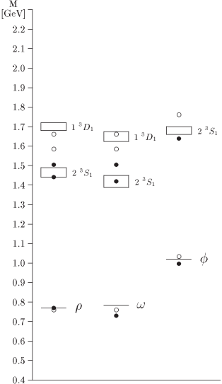
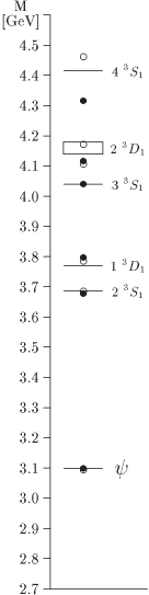
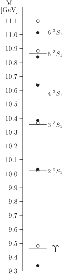
FIG. 1.: Comparison of the DNR and $\chi$QM spectra for $J^{P}=1^{-}$ resonances discussed in the text. The horizontal lines indicate the experimental values of the masses, being rectangles in the case of an experimental uncertainty bigger than 20 MeV, the open circles show the values obtained with DNR potential and the dark circles those from $\chi$QM potential. The $\rho$($n\bar{n}$ system, I=1), $\omega$($n\bar{n}$ system, I=0), $\phi$($s\bar{s}$ system) families have a common scale whereas $\psi$($c\bar{c}$ system) and $\Upsilon$($b\bar{b}$ system) families have their own one. The spectroscopic quantum numbers are indicated close to the experimental mass values.

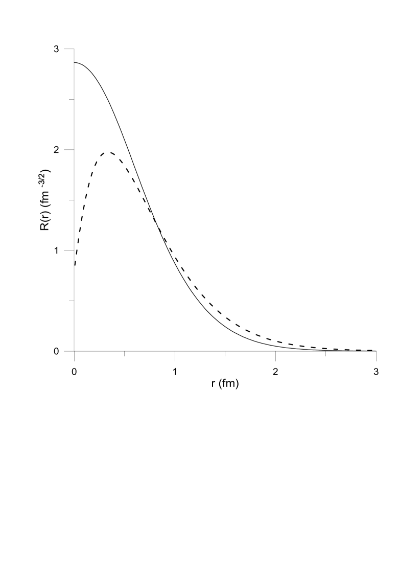
FIG. 2.: Radial wave functions $R(r)$ of the $\rho$ meson obtained with DNR (solid line) and $\chi$QM (dashed line) potentials.

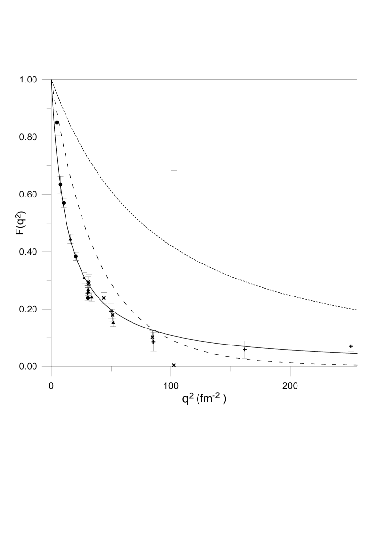
FIG. 3.: Pion charge form factor calculated with the $\chi$QM wave function. The dotted line corresponds to the bare quark calculation. Dashed line corresponds to the dressed quark calculation. Solid line includes the effect of boosting.

TABLE I.: Mean value $\langle\chi_{\lambda_{1}}|\sigma_{i}|\chi_{\lambda_{2}}\rangle$ of the Pauli matrices between helicity states.

$\lambda_{1}$	$\lambda_{2}$	$\sigma_{1}$	$\sigma_{0}$	$\sigma_{-1}$
$1/2$	$1/2$	$-\frac{\sin\theta}{\sqrt{2}}e^{i\varphi}$	$\cos\theta$	$\frac{\sin\theta}{\sqrt{2}}e^{-i\varphi}$
$1/2$	$-1/2$	$-\frac{1+\cos\theta}{\sqrt{2}}e^{i\varphi}$	$-\sin\theta$	$-\frac{1-\cos\theta}{\sqrt{2}}e^{-i\varphi}$
$-1/2$	$1/2$	$\frac{1-\cos\theta}{\sqrt{2}}e^{i\varphi}$	$-\sin\theta$	$\frac{1+\cos\theta}{\sqrt{2}}e^{-i\varphi}$
$-1/2$	$-1/2$	$\frac{\sin\theta}{\sqrt{2}}e^{i\varphi}$	$-\cos\theta$	$-\frac{\sin\theta}{\sqrt{2}}e^{-i\varphi}$

TABLE II.: Results for the widths with potentials $\chi$QM and DNR, in keV. Experimental data are from [21]. “V. R.” means application of the original van Royen-Weisskopf formula, “VRM.” means the formula taking into account the modifications given by Eq. (21), and “dressed” means that a gaussian distribution have been used to dress the quarks. The five last transitions ($\ast$) have a theoretical width $\Gamma_{\mu\mu}\simeq\Gamma_{ee}$, but the transitions to $\mu^{+}\mu^{-}$ have not been observed experimentally.

	DNR	$\chi$QM	DNR	$\chi$QM	DNR	$\chi$QM
transition	V. R.	V. R.	VRM.	VRM.	dressed	dressed	Exp.
$\rho\rightarrow e^{+}e^{-}$	11.360	0.998	8.601	1.315	5.719	3.648	6.75 $\pm$ 0.33
$\ \ \,\rightarrow\mu^{+}\mu^{-}$	11.335	0.996	8.582	1.312	5.707	3.640	6.91 $\pm$ 0.42
$\omega\rightarrow e^{+}e^{-}$	1.217	0.160	0.922	0.187	0.613	0.460	0.60 $\pm$ 0.02
$\ \ \,\rightarrow\mu^{+}\mu^{-}$	1.215	0.160	0.920	0.187	0.612	0.459	$<$1.52
$\phi\rightarrow e^{+}e^{-}$	2.984	0.982	2.464	0.964	1.643	1.214	1.30 $\pm$ 0.03
$\ \ \,\rightarrow\mu^{+}\mu^{-}$	2.982	0.981	2.462	0.963	1.642	1.213	1.65 $\pm$ 0.22
$J/\psi$(1S)$\rightarrow e^{+}e^{-}$	7.381	11.461	6.634	9.740	5.330	4.346	5.16 $\pm$ 0.31
$\ \ \ \ \ \ \ \ \ \ \ \rightarrow\mu^{+}\mu^{-}$	7.381	11.461	6.634	9.740	5.330	4.346	5.11 $\pm$ 0.31
$\psi$(2S)$\rightarrow e^{+}e^{-}$	3.696	4.603	3.101	3.697	2.074	1.075	2.44 $\pm$ 0.45
$\ \ \ \ \ \ \ \ \rightarrow\mu^{+}\mu^{-}$	3.696	4.603	3.101	3.697	2.074	1.075	2.85 $\pm$ 1.02
$\ \ \ \ \ \ \ \ \rightarrow\tau^{+}\tau^{-}$	1.436	1.788	1.204	1.436	0.806	0.418	not seen
$\psi$(4040)$\rightarrow e^{+}e^{-}$	2.681	2.904	2.175	2.273	1.300	0.507	0.73 $\pm$ 0.25
$\ \ \ \ \ \ \ \ \ \ \rightarrow\mu^{+}\mu^{-}$	2.681	2.904	2.175	2.273	1.300	0.507	seen
$\ \ \ \ \ \ \ \ \ \ \rightarrow\tau^{+}\tau^{-}$	1.768	1.915	1.434	1.500	0.858	0.334	not seen
$\psi$(4415)$\rightarrow e^{+}e^{-}$	2.087	1.979	1.653	1.543	0.900	0.287	0.47 $\pm$ 0.24
$\ \ \ \ \ \ \ \ \ \ \rightarrow\mu^{+}\mu^{-}$	2.087	1.979	1.653	1.543	0.900	0.287	not seen
$\ \ \ \ \ \ \ \ \ \ \rightarrow\tau^{+}\tau^{-}$	1.640	1.554	1.298	1.212	0.707	0.225	not seen
$\psi$(3770)$\rightarrow e^{+}e^{-}$	0	0	0.023	0.019	0.017	0.009	0.26 $\pm$ 0.05
$\ \ \ \ \ \ \ \ \ \ \rightarrow\mu^{+}\mu^{-}$	0	0	0.023	0.019	0.017	0.009	not seen
$\ \ \ \ \ \ \ \ \ \ \rightarrow\tau^{+}\tau^{-}$	0	0	0.011	0.009	0.008	0.004	not seen
$\psi$(4160)$\rightarrow e^{+}e^{-}$	0	0	0.032	0.023	0.021	0.009	0.78 $\pm$ 0.37
$\ \ \ \ \ \ \ \ \ \ \rightarrow\mu^{+}\mu^{-}$	0	0	0.032	0.023	0.021	0.009	not seen
$\ \ \ \ \ \ \ \ \ \ \rightarrow\tau^{+}\tau^{-}$	0	0	0.023	0.016	0.015	0.006	not seen
$\Upsilon$(1S)$\rightarrow e^{+}e^{-}$	1.415	5.052	1.299	4.291	1.287	2.727	1.25 $\pm$ 0.07
$\ \ \ \ \ \ \ \ \rightarrow\mu^{+}\mu^{-}$	1.415	5.052	1.299	4.291	1.287	2.727	1.30 $\pm$ 0.06
$\ \ \ \ \ \ \ \ \rightarrow\tau^{+}\tau^{-}$	1.404	5.012	1.288	4.257	1.277	2.706	1.40 $\pm$ 0.09
$\Upsilon$(2S)$\rightarrow e^{+}e^{-}$	0.654	1.496	0.588	1.252	0.583	0.742	0.52 $\pm$ 0.12
$\ \ \ \ \ \ \ \ \rightarrow\mu^{+}\mu^{-}$	0.654	1.496	0.588	1.252	0.583	0.742	0.58 $\pm$ 0.13
$\ \ \ \ \ \ \ \ \rightarrow\tau^{+}\tau^{-}$	0.650	1.487	0.585	1.244	0.580	0.737	0.75 $\pm$ 0.71
$\Upsilon$(3S)$\rightarrow e^{+}e^{-}$	0.488	0.922	0.432	0.765	0.428	0.446	seen
$\ \ \ \ \ \ \ \ \rightarrow\mu^{+}\mu^{-}$	0.488	0.922	0.432	0.765	0.428	0.446	0.48 $\pm$ 0.08
$\ \ \ \ \ \ \ \ \rightarrow\tau^{+}\tau^{-}$	0.485	0.917	0.430	0.761	0.426	0.444	not seen
$\Upsilon$(4S)$\rightarrow e^{+}e^{-}$	0.402	0.682	0.353	0.556	0.350	0.326	0.39 $\pm$ 0.17
$\ \ \ \ \ \ \ \ \rightarrow\mu^{+}\mu^{-}$	0.402	0.682	0.353	0.556	0.350	0.326	not seen
$\ \ \ \ \ \ \ \ \rightarrow\tau^{+}\tau^{-}$	0.400	0.679	0.352	0.553	0.348	0.324	not seen
$\Upsilon$(5S)$\rightarrow e^{+}e^{-}$	0.351	0.528	0.306	0.424	0.303	0.252	0.31 $\pm$ 0.08
$\ \ \ \ \ \ \ \ \rightarrow\mu^{+}\mu^{-}$	0.351	0.528	0.306	0.424	0.303	0.252	not seen
$\ \ \ \ \ \ \ \ \rightarrow\tau^{+}\tau^{-}$	0.349	0.526	0.305	0.422	0.301	0.251	not seen
$\Upsilon$(6S)$\rightarrow e^{+}e^{-}$	0.208	0.432	0.179	0.347	0.161	0.207	0.13 $\pm$ 0.05
$\ \ \ \ \ \ \ \ \rightarrow\mu^{+}\mu^{-}$	0.208	0.432	0.179	0.347	0.161	0.207	not seen
$\ \ \ \ \ \ \ \ \rightarrow\tau^{+}\tau^{-}$	0.207	0.430	0.178	0.346	0.160	0.206	not seen
$\omega(1420)\rightarrow e^{+}e^{-}$	0.363	0.039	0.233	0.033	0.094	0.041	seen $\ast$
$\rho(1450)\rightarrow e^{+}e^{-}$	3.063	0.202	1.970	0.192	0.794	0.326	seen $\ast$
$\omega(1650)\rightarrow e^{+}e^{-}$	0	0	0.021	0.012	0.011	0.009	seen $\ast$
$\phi(1680)\rightarrow e^{+}e^{-}$	1.010	0.280	0.722	0.231	0.278	0.172	seen $\ast$
$\rho(1700)\rightarrow e^{+}e^{-}$	0	0	0.179	0.094	0.091	0.077	seen $\ast$

REFERENCES

- [1] R. Bonnaz, L.A. Blanco, B. Silvestre-Brac, F.Fernández, A. Valcarce, Nucl. Phys. A 683 (2001) 425.
- [2] R. van Royen, V.F. Weisskopf, Nuovo Cimento A 50 (1967) 617.
- [3] B. Margolis, R.R. Mendel, Phys. Rev. D 28 (1983) 468.
- [4] N. Barik, P.C. Dash, A.R. Panda, Phys. Rev. D 47 (1993) 1001.
- [5] M. Beyer, U. Bohn, M.G. Huber, B.C. Metsch, J. Resag, Z. Phys. C 55 (1992) 307.
- [6] S. Louise, J.-J. Dugne, J.-F. Mathiot, Phys. Lett. B 472 (2000) 357.
- [7] F. Fernández, A. Valcarce, U. Straub, A. Faessler, J. Phys. G 19 (1993) 2013; D.R. Entem, F. Fernández, A. Valcarce, Phys. Rev. C 62 (2000) 034002.
- [8] D.A. Varshalovich, A.N. Moskalev, V.K. Khersonskii, Quantum Theory of Angular Momentum, World Scientific, Singapore, 1988, pg. 180.
- [9] M. Jacob, G.C. Wick, Ann. Phys. 7 (1959) 404; A.D. Martin and T.D. Spearman, Elementary Particle Theory, North-Holland, Amsterdam, 1970, pg. 124.
- [10] U. Vogl, M. Lutz, S. Klimt, W. Weise, Nucl. Phys. A 516 (1990) 469.
- [11] A. Buchmann, E. Hernández, K. Yazaki, Nucl. Phys. A 569 (1994) 661.
- [12] G. Wagner, A. Buchmann, Amand Faessler, Phys. Lett. B 359 (1995) 288.
- [13] A. Buchmann, E. Hernández, Amand Faessler, Phys. Rev. C 55 (1997) 448.
- [14] F. Cardarelli et al., Phys. Lett. B 357 (1995) 267.
- [15] F. Cardarelli et al., Phys. Lett. B 359 (1995) 1.
- [16] H. Garcilazo, A. Valcarce, F. Fernández, Phys. Rev. C 63 (2001) 035207.
- [17] L.A. Blanco, F. Fernández, A. Valcarce, Phys. Rev. C 59 (1999) 438.
- [18] C. Semay, B. Silvestre-Brac, Nucl. Phys. A 618 (1997) 455.
- [19] D.P. Stanley, D. Robson, Phys. Rev. D 26 (1982) 223.
- [20] S. Weinberg, The Quantum Theory of Fields, Cambridge Univ. Press, New York, 1995, pg. 136.
- [21] D.E. Groom et al., Eur. Phys. J. C 15 (2000) 1.