Observing Spontaneous Strong Parity Violation in Heavy-Ion Collisions

Abstract

We discuss the problem of observing spontaneous parity and CP violation in collision systems. We discuss and propose observables which may be used in heavy-ion collisions to observe such violations, as well as event-by-event methods to analyze the data. Finally, we discuss simple monte-carlo models of these CP violating effects which we have used to develop our techniques and from which we derive rough estimates of sensitivities to signals which may be seen at RHIC.

I Introduction

Parity and CP symmetries have been a source of fascination to physicists since the discoveries that neither is absolutely respected by nature. [1, 2]. To date, the violation of these symmetries has only been observed in weak interactions, never in strong or electromagnetic interactions. Why the CP symmetry should normally be respected by the strong interaction, as seems to be the case experimentally, is an outstanding mystery (the so-called strong CP problem [3]), but a topic separate from this paper.

Kharzeev et. al. [4] have proposed that even if the strong interactions normally respect CP symmetry (or in the language of the field, even if $\bar{\theta}_{QCD}$ [3] is equal to zero), that in hot hadronic matter, metastable states may be formed in which parity and CP are spontaneously violated.

The authors obtained this result using a non-linear sigma model as an effective Lagrangian, explicitly including a term which incorporates the breaking of the axial U(1) symmetry which is present in Quantum Chromodynamics. They have found that within the context of this model, under certain assumptions about the nature of deconfining and chiral phase transitions, metastable states may form which behave as regions in which $\bar{\theta}_{QCD}$ is nonzero, and so spontaneously break CP symmetry. They then further proposed that such regions may be produced in relativistic collisions of heavy nuclei. (The possibility of CP violating vacuum states formed in heavy ion collisions is not tied to this mechanism and in fact the general idea was raised several years prior [5].)

In Reference [4] and subsequent papers [6, 7, 8, 9, 10], methods for observing CP violating states in heavy ion collisions have been suggested which can be grouped into two categories based upon the proposed experimental signatures. The first group of signatures have to do with the observation of parity violating strong decays which are normally forbidden and with the observation of anomalous particle production [8, 9, 10]. The second group have to do with direct observation of global parity and CP odd observables which may be formed out of the momenta of final state particles. It is with this second group of signatures that we are concerned in this paper.

Two mechanisms have been proposed by which strong CP violation can lead to observable effects in global variables formed from the momentum vectors of the final state particles. The first is that one of these metastable regions which varies in time may give rise to a CP violating asymmetry in $\pi^{+}$ and $\pi^{-}$ momenta. This is discussed in Reference [6] as arising through the ’Witten-Wess-Zumino Term’ [11, 12] and led to the proposal for the event-by-event observable

$$J=\frac{1}{N_{pairs}}\sum_{pairs}[\hat{p}_{+}\times\hat{p}_{-}]\cdot\hat{z}$$ (1)

where the sum is over all possible pairs and each pair contains one observed $\pi^{+}$ and one observed $\pi^{-}$. $\vec{p}_{\pm}$ represents the momentum vector of an observed $\pi^{\pm}$ and $\hat{p}_{\pm}$ a unit vector in the same direction. $\hat{z}$ must be some other polar vector which can be defined in the collision system. (This particular observable will be discussed further in Section II.)

Additionally, because a nonzero value for $\bar{\theta}_{QCD}$ effectively implies a nonzero value for $\vec{B}_{c}\cdot\vec{E}_{c}$ (where these are chromo-magnetic and chromo-electric fields) [6, 3], it has been proposed [7] that this CP asymmetry would be manifested in CP-violating deflections of the trajectories of quarks which pass through these regions. This then should ultimately appear in CP-odd observables formed out of the momentum vectors of final state baryons rather than pions (because pions have equal fragmentation probabilities from light quarks and antiquarks).

A Spontaneous Parity Violation

Let us end this introduction with a few comments concerning the observation of symmetry violation in collision systems in general (specifically, what type of violations may or may not be demonstrated by the observations of non-zero value in a P or CP odd observable) and the added complications that are related specifically to spontaneous symmetry violation.

In a collision system consisting of two identical spin-0 nuclei, the initial state is an eigenstate of parity (in the center-of-mass system), which implies that no parity odd observable can have a nonzero expectation value with respect to this initial state. If the interaction respects parity symmetry, this must also be true of the final state; only if the interaction does not respect parity, producing a final state of mixed parity, can the final state show a non-zero expectation value for any parity-odd observable.

This conclusion is also true even if the collision system consists of two non-identical (spin-0) particles. Even assuming a nonzero impact parameter, only one pseudovector can be defined in the initial state, and it is (by its definition) orthogonal to the two available polar vectors. Therefore if we can form any pseudoscalar observable in the final state which has a nonzero expectation value, this demonstrates a violation of parity in the interaction.

If it is true that an expected signal due to parity violation is too small to be observed in a single event, as it is here, then one must clearly look for a cumulative effect over many events. If the interaction violated parity in the same manner for every event (for example if $\vec{B}_{c}\cdot\vec{E}_{c}$ were for every event greater than zero rather that simply nonzero), then the effect would accumulate over many events and a nonzero mean for the distribution of some event-by-event parity odd operator could be observed as proof of parity violation. If however, as is the case here, the effect is spontaneous and changes handedness randomly from event to event with equal probability to be left or right handed, then the average value over many events for a parity odd observable must be zero. In this case the only signatures of the violation we can observe are in the widths of event-by-event distributions of P-odd observables. More discussion of this point and the methods by which the observation of this change in a distribution’s width can best be accomplished is found in Section IV.

And finally there are two important notes concerning what symmetry violations can actually be demonstrated in this collision system. Clearly, the initial state consisting of two nuclei can not be an eigenstate of charge conjugation and so our initial state can not have definite CP properties. Therefore we can not demonstrate CP violation by observing final states of mixed CP properties by the same argument as given above for parity. However, the nature of the expected CP violation can and should lead us in our choice of parity odd observables. Time reversal violation (related of course to CP violation by the CPT theorem) could in principle be determined by constructing final state observables odd under motion reversal but this is complicated by T-odd final state phase shifts of the outgoing particles’ momenta[13].

The second point to note is that if the initial state nuclei are not spin zero, then the initial state in a given event is not a parity eigenstate and there generally will be nonzero pseudoscalar observables which can be constructed from the initial state. For unpolarized beams, this can in principle lead to a nonzero expectation value for a parity odd observable in each event which may change the widths of these event-by-event distributions and be mistaken for the signature of spontaneous symmetry violation. We will come back to this point again later with specific observables and a range of observed final state momenta in mind, but of course this point is most effectively dealt with by colliding beams of spinless nuclei such as Pb(208).

II Observables-Old and New

As defined in Equation 1 and suggested in reference [4], the observable $J$ is problematic. For $J$ to be parity odd, $\hat{z}$ must be a real (polar) vector and so must correspond to some uniquely definable direction. The initial suggestion of the $z$ direction as the beam axis is useful only for collisions of non-identical particles for which this can be uniquely defined.

This problem can be rectified as suggested in [6] by replacing $\hat{z}$ with a real vector which measures either the particle flow ($\vec{k}_{+}$) or the charge separation ($\vec{k}_{-}$) of a given event. These vectors can be defined using the final state particles’ momentum vectors as

$$\vec{k}_{\pm}=\frac{1}{N_{+}}\sum_{+}\hat{p}_{+}\pm\frac{1}{N_{-}}\sum_{-}\hat{p}_{-}$$ (2)

where the factors $N_{\pm}$ are simply the numbers of observed $\pi^{\pm}$ and the sums run over all observed pions of a given species in an event. (We will speak about pions in this section for definiteness but as discussed in Section I we can also define and have studied the same observables for protons and antiprotons). Making this replacement of $\vec{k}_{-}$ for $\hat{z}$, we have an experimentally definable operator which is odd under parity, time reversal and CP.

However, for identical particle collisions, the event sum $\sum_{pairs}(\hat{p}_{+}\times\hat{p}_{-})$ results in a vector which has an additional fault which can be demonstrated as follows: Let the distribution of a given species of particles emitted from an event be called $g(\theta,\phi)$ where theta is the polar angle with respect to the beam axis and $\phi$ is the azimuthal angle. Then for central collisions on average $g(\theta,\phi)$ is azimuthally symmetric and $g(\theta)$ = $g(\theta+\pi)$. By modelling the momentum kicks that particles receive from the CP violating fields as angular rotations in momentum space with opposite charged species being rotated in opposite directions (See Figure 1 and related discussion later in this section), the contributions to $J$ from various parts of the $\pi^{+},\pi^{-}$ momentum space exactly cancel one another so that the total sum over all of momentum space is zero [14]. For any given event, these symmetries of $g(\theta,\phi)$ will be only approximately realized due to finite statistics (and directed flow interferes for non-central collisions), but to a large degree this effect still persists so that the observable $J$ is forced to be nearly zero by these approximate symmetries. This leads to $J$ as an observable being relatively insensitive to the effects of CP violation, and we have noted this effect in the results of our simulation models.

An observable which is similar to $J$ but which is not forced to zero by these symmetry constraints is a tensor observable previously proposed in reference [7] defined as

$$T_{ij}=\frac{1}{N_{pairs}}\sum_{pairs}[\hat{p}_{+}\times\hat{p}_{-}]\cdot{\hat{n}_{i}}[\hat{p}_{+}-\hat{p}_{-}]\cdot{\hat{n}_{j}}$$ (3)

Here $\hat{n}_{j}$ refers to a unit vector in the $j$th direction. $T_{ij}$ is manifestly P and CP odd, since the cross product yields an axial vector and the difference of two momentum vectors is a polar vector (the unit vectors are axial vectors). The diagonal components of this tensor are sensitive to the sorts of symmetry violation which $J$ was constructed to see; here we will only discuss $T_{zz}$. Each term in the sum which comprises $T_{zz}$ contributes a value which is roughly speaking a measure of the correlation between the longitudinal momentum difference of the pair and the azimuthal angle difference of the pair.

If the sum in Equation 3 is interpreted to be a sum over all possible pair combinations in an event, then the sum for each component of the tensor may be rewritten as a combination of single particle sums rather than a sum over pairs. For example,

$$T_{zz}=\langle\hat{p}_{x}\hat{p}_{z}\rangle_{+}\langle\hat{p}_{y}\rangle_{-}+\langle\hat{p}_{x}\hat{p}_{z}\rangle_{-}\langle\hat{p}_{y}\rangle_{+}-\langle\hat{p}_{y}\hat{p}_{z}\rangle_{+}\langle\hat{p}_{x}\rangle_{-}-\langle\hat{p}_{y}\hat{p}_{z}\rangle_{-}\langle\hat{p}_{x}\rangle_{+}$$ (4)

where for example $\langle p_{x}p_{z}\rangle_{+}$ is short hand for $\frac{1}{N_{+}}\sum_{+}(\hat{p}_{+}\cdot\hat{x})(\hat{p}_{+}\cdot\hat{z})$. This form of $T_{zz}$ has a clear computational advantage for experiments which may have thousands of particles, and therefore millions of possible pairs, in a given event.

$T_{zz}$ also has a very natural interpretation when used, as it was originally intended, to observe momentum space asymmetries among baryons. If we consider the CP violation as being caused by aligned chromoelectric and chromomagnetic fields, we can visualize the effects of these fields in momentum space on the distributions of quarks and antiquarks (or, after hadronization, protons and antiprotons). In the absence of CP violation we imagine that the two different species fill approximately the same ellipsoid in momentum space, elongated along the beam ($z$) axis. With the addition of these CP violating fields, however, the ellipsoids are (roughly speaking) displaced to a form such as that shown in Figure 1. The chromoelectric field moves the two species apart along the direction of the field, and the chromomagnetic field rotates the two species’ momentum space distributions in opposite directions around the field axis (note that if we assume that the momentum distribution of particles in the bubble were isotropic then no effect would be observable). It is this combined action of the ’lift’ along the field axis with the ’twist’ around the field axis which $T_{zz}$ is sensitive to.

This picture also leads to the idea that equation 4 may be rewritten in a coordinate system defined by the charge flow axis ($\hat{k}_{-}$), and then it may be beneficial to selectively keep only those terms from Equation 4 which lay along this axis. This process yields a different observable,

$$K_{twist}=\frac{1}{N_{+}}\sum_{+}(p_{y}k_{-,x}-p_{x}k_{-,y})-\frac{1}{N_{-}}\sum_{-}(p_{y}k_{-,x}-p_{x}k_{-,y})$$ (5)

where the vector $\vec{k}_{-}$ is defined by Equation 2.

We can also slightly alter the construction of $J$ and so create a different pseudoscalar observable which is not forced to zero by symmetry considerations. We simply introduce into each term of the sum which defines $J$ a factor which depends on the relative momentum space position of the the two pions involved. Specifically, an extra factor of $-1$ is introduced depending on whether the two pion momenta are in the same or opposite directions with respect to the beam (z) axis in the collision center-of-mass frame. Following this prescription we can then define the vector $\vec{J_{c}}$ as

$$\vec{J}_{c}=\frac{1}{N_{pairs}}\sum_{pairs}[(\hat{p}_{+}\times\hat{p}_{-})sgn(p_{z,+}p_{z,-})]$$ (6)

and we note that the scalar $\vec{J}_{c}\cdot\vec{k}_{-}$ is a P and CP odd observable which we propose as another alternative to $J$, intended to capture the same physics without its practical difficulties.

And finally, we have also studied the observable proposed in reference [15] defined as

$$V_{+}=(\langle\vec{p}_{t}\rangle_{+,y>y_{cm}}\times\langle\vec{p}_{t}\rangle_{+,y<y_{cm}})\cdot\hat{z}$$ (7)

(Here, $\hat{z}$ is a unit vector along the z axis which is chosen arbitrarily along one of the beam directions, and so is an axial vector.) This observable has the advantage that it can be defined for a single particle species (as written, it only involves $\pi^{+}$) and so avoids assumptions about how particles and antiparticles will be affected differently by the fields. A disadvantage is the resulting assumption that the particles with rapidity greater than $y_{cm}$ will be deflected oppositely to those travelling in the opposite direction (tantamount to assuming that the CP violating region will generally sit at $y=y_{cm}$).

We have found from our model simulations (see Sections III and V) that under most circumstances these observables behave quite similarly and generally do not differ from one another in sensitivity by more than a factor of a few in any given situation, with none of them being systematically better than the others. It will likely be useful to study experimental data with all of them, as they do provide useful cross checks on one another and of course a factor of a few in statistics is not to be taken lightly. We do not discuss here other proposed observables such those defined in [6] because we have not studied these in any detail.

III Simulation Models

In order to develop these observables as well as to make rough estimates of the sensitivity that we may expect a RHIC experiment to have to these effects, we have developed some simple models to simulate the effects of the proposed strong CP violation. These models are not intended to be realistic descriptions of the collision and CP violating dynamics, but rather to lead to similar final state asymmetries which we can use to estimate observable signals.

We base Model $I$ on the idea that the CP violating region will exist as a ’bubble’ inside the collision region which contains a nonzero value of $\vec{E}\cdot\vec{B}$. These fields then affect the trajectories of quarks or hadrons which pass through this bubble. We model the color fields as electromagnetic fields and so let them provide forces by acting on the electric charges of the particles; thus mimicking the net effect that the strong fields would have on the particles’ trajectories. Modelling the fields in this manner is an assumption but we believe not an unreasonable one in light of the discussion in Section I concerning the predicted net effects that the color forces will have on the pion and baryon momentum spectra.

The initial distribution of particles in momentum space for Model $I$ is taken from the event generator HIJING [16]. Initial positions for these particles are then picked randomly from a uniform distribution over a spherical collision volume (note than no position-momentum correlations are included in this simple model). The CP violating bubble is then included as a static, randomly positioned spherical sub-region of this collision volume in which there are nonzero aligned electric and magnetic fields. As charged particles move from their initial positions, if they happen to cross through this CP violating bubble their trajectories are altered by the presence of the aligned fields. The field strength and size of these regions is chosen to correspond to theoretical predictions about these CP violating regions and their color fields; they are determined as described in Section V.

Additionally, to explore the idea advocated in [7] of examining the trajectories of final state baryons rather than pions, the model is altered in the following way for further studies: The initial proton and antiproton distributions are again taken from HIJING. Each baryon is decomposed into its constituent quarks which are then spread through the collision region. After each quark is allowed to traverse the CP violating bubble, if appropriate given its initial position and trajectory, the quarks are re-coalesced into a baryon, which as a result of this process receives a net momentum kick equal to the sum of the kicks given to the constituent quarks.

To summarize then, we model the fields as producing opposite impulses on oppositely charged particles, producing CP violating asymmetries in both pionic and proton-antiproton observables. (Probably the mechanism is somewhat closer to the truth for $p/\bar{p}$ where the proposed color fields really should act oppositely on the different species. For pions, we may simply view this mechanism as a way to produce the expected asymmetries caused by CP violation).

Models $II$ and $III$ are similarly based on the idea of embedding into events metastable bubbles which have a vacuum where CP is violated. For these models, we use RHIC::EVENT[19] (an improved version of HIJET[20]) as the basic event generator.

This generator was then customized for CP violation studies. In each generated event, the particles within a certain spatial region are ’tagged’ to be turned into a bubble with CP violating vacuum (for details see[19]) which has the momentum and baryon numbers of the particles it replaces. This bubble consists of quarks uniformly distributed in a region of aligned color electric and magnetic fields (of randomly chosen direction) that alter the quarks’ momentum similarly to what was described for pions in model $I$ (oppositely for quarks and antiquarks). When a quark reaches the boundary of the bubble, it forms a pion which retains the effect of the impulse imparted to the quark from the color fields (again, for details see[19]). For these models, the expected net flow of pion charge [6] is obtained by allowing the momentum impulses given to quarks to affect positive pions and the impulses given to anti-quarks to affect only negative pions.

Using this underlying model, we have studied the effects of different assumptions concerning the momentum distributions of pions emitted from the bubble. Two assumptions that were studied were a spherically symmetric Boltzmann distribution with a temperature of 70 MeV (this is Model $II$), and a Landau expansion with a transverse temperature of 150 MeV and a distribution along the beam axis which is flat over four units of rapidity (Model $III$).

For Model $II$, if the color fields are of uniform strength throughout the bubble, no signal due to the fields’ effects may be seen on the final momentum of the pions (imagine Figure 1 with initially spherically symmetric distributions in momentum space, so that the rotation caused by the color magnetic field could not be detected.). In this case we have broken this symmetry by making the field strengths constant only in the transverse direction and letting them have a strong longitudinal dependence. For Model $III$, as in Model $I$, the necessary asymmetry is built in to the pion momentum distribution, so that such a field dependence need not be assumed.

To obtain quantitative results from these models concerning sensitivities at RHIC, we assume an acceptance of -1 to +1 in rapidity and .120 to 1 GeV/c in transverse momentum, similar to that of STAR [17].

IV Experimental Methods

As described in Section I, the spontaneous nature of this proposed CP violation makes it impossible to see a nonzero expectation value in the distribution of any CP odd observable which will accumulate from event to event. This, combined with the fact that we expect any single event to have far too small a signal to be statistically significant (this is clearly confirmed by our model simulations even under extreme assumptions about the strength of the CP violation), means we have to turn to event-by-event techniques to look for a signal.

Because any signal of spontaneous CP violation will be contained essentially in the width of the event-by-event distributions of CP odd observables (as illustrated is Figure 2 ) such as those described above, the most straightforward method is to measure the width of one of these distributions and compare it to a reference ’no-signal’ distribution. Of course, then the problem becomes one of how to create a bias free reference distribution with which we can compare.

A Mixed Event Reference Distributions

Perhaps the easiest way to create a reference distribution is to use real events to create a pool of ”mixed-events”. These are fake events which are constructed from small pieces (ideally, just one track) taken from many different real reconstructed events. In this manner one creates a pool of mixed events which have the global features of real events but absent any of the correlations between tracks, including those caused by CP violation. Thus in the presence of CP violation, the distribution of values of any of our observables should be wider in real events than it is in mixed events.

The presence or absence of a signal for parity violation can be determined quantitatively in this method then by simply forming histograms of the distribution of (for example) $T_{zz}$ for real events and for mixed events and then taking the difference of these two histograms. This difference histogram can then be compared channel by channel with a value of 0 and a $\chi^{2}$ value obtained for the difference. If this process were repeated many times on signal-free independent samples of equal size, the values of $\chi^{2}$ should form a gaussian distribution about the number of degrees of freedom ($N_{dof}$) in the fit with a width given by $\sqrt{(}2N_{dof})$ (this is assuming a sufficiently large number of non-zero bins). For any single data sample then, the value $(\chi_{2}-N_{dof})/\sqrt{(}2N_{dof})$ gives a quantitative measure of the number of standard deviations away from zero signal. This measure does depend somewhat on the binning chosen for histograms, but the variations for any reasonable choice of binning tends to be well less than a factor of 2.

In our simulation models, using this method with any of the observables described above shows by far the largest signal in the presence of CP violating bubbles of any method we have tried, but this is quite misleading: Any effect which makes the momentum space structure different in real events than in mixed events can in principle lead to a signal in this method. This certainly includes practical experimental effects which will be discussed in Section VI. However, this also includes other physics effects such as the presence of jets and fluctuations of mean $p_{T}$ in real events. Additionally, a positive signal using any of the observables described above can be produced by the presence of a nonzero $\vec{B}$ field without a correlated $\vec{E}$, or vice versa. (This signal is due to a change in the width of the distributions that comes about not because a slightly nonzero mean in each event is added on top of fluctuations as would be the case for correlated $\vec{B}$ and $\vec{E}$, but simply because the presence of a single field causes the size of the event-by-event fluctuations about zero to increase) ; one field alone does not imply a CP violation but does produce a signal in this mixed event method.

This final point is somewhat subtle so we will attempt to clarify it, using $\vec{J}_{c}\cdot\vec{k}^{-}$ for definiteness. If the real event distribution of $|\vec{k}_{-}|$ has an rms width larger than the same distribution from mixed events (which it does in our simulations if we turn on only an $\vec{E}$ field since this is essentially what $k^{-}$ measures), this by itself will give a larger width to the distribution of $\vec{J}_{c}\cdot\vec{k}^{-}$ in real compared with mixed events, without any event-by-event correlation in the directions of the two vectors in real events. We could in principle avoid this problem by switching to an observable such as $\hat{J}_{c}\cdot\hat{k}^{-}$ which measures only the angular correlation between the two vectors, but this is more effectively done by changing the way in which the reference distributions are made to the method described in Section IV C

We conclude then that using the mixed event method as here described might be useful to set an upper limit in the absence of a signal (if some non-trivial practical problems can be overcome), but the observation of a signal using this technique could never by itself be taken as strong evidence for parity violation.

B Subevents

A second method, which for our purposes is much more robust, is another standard event-by-event technique generally referred to as the Subevent Method [18]. The method is quite simple: we in some manner parse the tracks from an event into two subevents and calculate the value of one of our observables, say $K_{twist}$, for each subevent. To look for a signal then, we look at whether there is a significant covariance between the distributions of $(K_{twist})_{sub1}$ and $(K_{twist})_{sub2}$. Equivalently, we can observe the distribution of event-by-event values of $(K_{twist})_{sub1}\cdot(K_{twist})_{sub2}$. If the mean of this distribution is significantly shifted away from zero, a parity violation is implied.

The idea behind this method then is this: the expectation value of $(K_{twist})$ in any event or subevent in which parity is not violated will be zero (and the distribution of values should be symmetric about zero). So if we choose two random uncorrelated subevents from an event and calculate $K_{twist}$ for each of these, we randomly sample two such distributions, and $(K_{twist})_{sub1}\cdot(K_{twist})_{sub2}$ should then also be symmetrically distributed about zero. If ,however, there is CP violation in an event, we expect both subevents to yield values for $(K_{twist})$ which are on average shifted slightly in the same direction, yielding a distribution for $(K_{twist})_{sub1}\cdot(K_{twist})_{sub2}$ which, given enough events, will have a mean significantly greater than zero.

Different methods of choosing subevents have their own advantages and disadvantages as discussed briefly in [18]. Two possible variations are (i) Choosing the subevents randomly from the available tracks, and thus forming two subevents which overlap in momentum space. (ii) Dividing an event into subevents by partitioning momentum space, ideally with some gap in momentum space between the two. Because the parity violation may be localized in momentum space, variation (i) may have an advantage in sensitivity in real data. Variation (ii) however, has a clear advantage in avoiding correlations between the two subevents, and for a study such as this where a false signal is clearly highly undesirable this is an important advantage. Also, (ii) may be easily generalized to a larger number of smaller subevents per event which in principle is useful for looking for parity violating correlations over a momentum range smaller than an entire event.

The subevent method avoids most of the pitfalls of the mixed event method discussed above, but the price is that it takes significantly more events to produce an effect in the subevent method. (Just to clarify again: the underlying reason for this is that the subevent method in our simulations is sensitive only to the presence of aligned color $E$ and $B$ fields which implies CP violation; the mixed event method is sensitive not only to this, but also to the presence of only one of these fields, which does not by itself imply CP violation.) This will be discussed more quantitatively in Section V.

C Other Reference Distributions

There are other methods for producing reference distributions which avoid the problems of the mixed event method as described above. For example, when using a pseudoscalar observable which measures the event-by-event correlation of two vectors (we’ll use $\vec{J}_{c}\cdot\vec{k}_{-}$ as an example), one can form the reference distribution by using the vector $\vec{J}_{c}$ from a given event and the vector $\vec{k}_{-}$ from a different event; there are several similar variations of this method which retain this basic principle. We find this technique to be similar to the subevent method in its sensitivity to CP violation, and it is similarly not sensitive to the false signals that the mixed event method is.

V Simluation Results and Expected Sensitivities

For our studies with model $I$, the size of the CP violating region and the strength of the fields in this region can be varied for a systematic study of the signal strength as a function of these parameters, and some of the results from these studies are shown in Table I. Clearly, there is considerable uncertainty in choosing reasonable values for these parameters. The nominal value for the field strength we have taken as suggested by D. Kharzeev [21]; both $E$ and $B$ fields are strong enough to give a 30 MeV/c kick in momentum to a relativistic quark which traverses the length of the region (for simplicity, from now on we will write field strengths in units where this value is equal to one). For the bubble size, our nominal choice is to use a bubble radius equal to 1/5 or 2/5 of the radius of the ’collision region’. These sizes are chosen so that the fields affect about 100 pions in an event, as suggested in [6]. We list in Table  I the approximate number of RHIC Au+Au events that were required in our simulations to produce an effect from CP violation at the $3\sigma$ level in the observable $T_{zz}$. We also list results for other larger choices of bubble size and field strength mainly to demonstrate the scaling of the number of required events versus these parameters. In the subevent case, we find that the strength of the signal (as measured by shift of the distribution mean away from zero) scales as the field strength to the fourth power, as expected; the value of these observables is affected linearly by the strength of both the $E$ and $B$ fields and the shift of the subevent distribution scales as the square of the event-wise distribution. Recall that as discussed in Section IV, although the mixed-event method is clearly the more sensitive, a signal in this method could not be taken as strong evidence for parity violation.

Although we show only the results for $T_{zz}$ in this table, the results for $K_{twist}$, $V$, and $\vec{J}_{c}\cdot\vec{k}_{-}$ are roughly consistent with these; variations on the order of factors of a few between the observables in some cases are observed.

In Table II we show a comparison between the predictions of the three different models with comparable choices of field strength and bubble sizes. The nominal values used for models $II$ and $III$ were established in a similar manner to those for model $I$, with the bubble size chosen again so that approximately 100 pions are produced by quarks exiting the bubble. For the comparison shown here we have used a bubble radius of 1/5 in Model $I$ and the actual observable compared is $K_{twist}$. This comparison gives some idea of the variations we can obtain even from somewhat similar models: model $II$ (non-uniform field strength in the longitudinal direction) predicts considerably better sensitivity than Model $I$, while Model $III$ (pions with a Landau distribution) gives us results more similar to model $I$.

We see from Tables I and II that even with the mixed event method, we would not expect to see any signs of the presence of CP violation with less than a few$\times 10^{5}$ central RHIC events. For strong evidence of parity violation (meaning a signal with the subevent method or a using a more robust reference distribution method) the number of events needed seems to be more like a minimum of a few $\times 10^{7}$ central RHIC events.

Some comments about these results are in order. Firstly, we emphasize again that the transition from the theory advocated in [4] to these models requires several assumptions and if these are changed the results could be quite different. For example, we can also choose for nominal values of the bubble size and strength those values which would produce a signal at the $10^{-3}$ level in the observable $J_{c}$ for pion pairs coming from the bubble (as suggested in [6]) as opposed to the $10^{-2}$ level which is produced by model $I$ using the parameters from the top row of Table I; this would clearly lead to a considerably more pessimistic outlook for the number of events needed.

Finally, we should mention our results from using model $I$ to model the effects on protons and antiprotons as described in Section III. Clearly, the main drawback in using baryons rather than pions is the small relative number produced in the collision. In the case of bubble radius = 2/5 and field strength of 1 (the more optimistic ’nominal’ case from above) this model predicts that we could observe a $3\sigma$ signal using the mixed event method in approximately 3 million central events (compared to about 300K events with pions). We conclude then that we have little chance of observing a CP violation signal for protons and antiprotons, particularly using any of the more robust methods.

VI False Signals

Of course a very important point in studies such as these is the possibility of something other than actual parity violation faking a positive signal.

A Experimental Inefficiencies

Experimental inefficiencies may be divided into two categories: Single track inefficiencies and correlated inefficiencies.

We have attempted to simulate various patterns of single track inefficiencies as a function of polar and azimuthal angle as well as differing inefficiencies for different charge species and have been unable to produce a fake signal of any sort from these effects alone. Furthermore, even if a pattern exists which can cause a fake signal, provided that it is static in time, it clearly should not behave as a signal which changes handedness event-to-event and therefore should be observable as a shift of the mean of the event-by-event distributions of our CP odd variables rather than just a broadening of these distributions. Considering these factors, we conclude that single track inefficiencies alone are not a significant concern for providing a false signal which is indistinguishable from a true parity violation (the same arguments also apply to single track measurement errors).

More concerning are correlated efficiencies, and specifically track merging and splitting (the results of track recognition software mistaking two nearby tracks for a single track or mistaking a single track for two similar tracks). Either of these can generally cause a fake signal for the mixed event method as can in principle any effect that makes the momentum space distribution of tracks different in real events compared with mixed events. This can to some extent be compensated for when forming mixed events, but this is a paramount practical concern about using the mixed event method.

In principle track splitting may also cause difficulties with the subevent method; clearly if one of the two versions of a split track is assigned to each of two subevents, the subevents will contain a correlation that may lead to correlations in their values for parity odd observables. This was mentioned in Section IV B as motivation for forming subevents which are separated from one another in momentum space; provided that both tracks resulting from a split track are contained within the same subevent, track splitting should not cause a false signal for the subevent method which we can not distinguish from a real signal.

B Physics concerns

With a cartoon similar to that shown in Figure 1, we can visualize in momentum space the combined effects of directed flow together with a charge separation which increases the radial momentum of one charge species while decreasing the other. The combined result of these effects and finite detector acceptance can mimic the ’twist’ shown in Figure 1, but not the ’lift’. This generally would still not be confused with a CP violating effect because for this confusion to occur there must be some additional effect which distinguishes ’up’ from ’down’ along the twist axis. The differentiation could in principle be provided by asymmetric acceptances and efficiencies but these effects should be identifiable (for example, creating mixed events only out of events with nearly common reaction planes and processing these events by the subevent method should also show a signal if the signal is caused by these effects but not if it is a true CP violation). And ultimately, any false effect which has flow as one of its root causes should be distinguishable by its known dependence on collision centrality [22].

It is also true that many hyperons will be produced in a typical central event and these do in fact undergo parity violating weak decays. However, this process alone should not be able to lead to a parity violating effect in global event observables unless some facet of hyperon production or polarization depends on production angle in a way that itself violates parity.

C Nuclei with Spin

If the two colliding nuclei are not spin zero, then it is no longer true that we can form no pseudoscalars in the initial state, and so it no longer follows that the expectation value of every pseudoscalar observable in any given collision is zero, but (provided the beams are not polarized), the average value over many events must still be zero. This, then, is a signal that may in principle appear in the ’width’ of the distribution of some pseudoscalar observable but not as a shifted mean value; exactly the type of effect we are concerned with observing. This is clearly a relevant point because the colliding beams at RHIC are composed of Au(197), a spin-(1/2) nucleus.

We should then consider what effect these initial state spins might have on the observables with which we are concerned here. For the observable $V$ defined in Equation 7, a left-right asymmetry in the production of $\pi^{+}$ and $\pi^{-}$ as is known to occur in polarized p-p collisions [23] is one mechanism by which nonzero spin could lead to an effect which would mimic CP violation. For example (labelling the two beam directions in a collision ’forward’ and ’backward’), if in a given collision forward going $\pi^{+}$ moved preferentially to the right with respect to the beam while backward moving $\pi^{+}$ moved preferentially down, this would lead to nonzero value for $V$ calculated from the $\pi^{+}$.

We can very roughly estimate the size of this effect using the available data [23] and the resulting phenomenological descriptions [24] to extrapolate to the momentum space region relevant for these studies. The asymmetry is characterized for a proton beam with spin measured to be ’up’ or ’down’ by

$$A_{N}=-\frac{1}{cos\phi}\frac{N_{\uparrow}(\phi)-N_{\downarrow}(\phi)}{N_{\uparrow}(\phi)+N_{\downarrow}(\phi)}$$ (8)

where $\phi$ is the angle between ’up’ and the pion production plane and $N_{\uparrow}(\phi)$ is the number of pions produced at $\phi$ when the proton is measured to have spin up. This asymmetry can be quite large in p-p collisions; typically, $A_{N}\approx$ 0.3 for $x_{F}\gtrsim 0.5$ and $p_{T}\gtrsim 700MeV/c$. However, for typical values of $x_{F}$ ($\lesssim$ 0.05) at $p_{T}$ ($\lesssim$ 1 GeV/c) that are appropriate here, the asymmetry is much smaller; we can take a conservative value of the asymmetry for $\pi^{+}$ as $10^{-2}$.

Using this value of $10^{-2}$ for $A_{N}$ of the $\pi^{+}$ and assuming the beams to be unpolarized, we can with our simulation models estimate the number of events needed to see a $3\sigma$ signal in $V_{+}$ due to this effect: In each event we randomly choose polarization vectors for the forward and backward beams. We then alter the event so that forward (backward) travelling $\pi^{+}$ have an asymmetry of $A_{N}=0.01$ with respect to the polarization direction of the forward (backward) travelling beam. We find that assuming an asymmetry of this size will give a $3\sigma$ signal for the subevent method in roughly $10^{9}$ events. Furthermore, this result is under the assumption that spin (1/2), A=200 nuclei will produce as large an asymmetry as a protons, which seems an extremely conservative assumption.

We conclude therefore that it is extremely unlikely that this particular mechanism presents a practical difficulty with the amount of data likely to be collected by RHIC experiments. We suspect that the this may be generally true of any CP-mimicking effects which may be caused by spin, because the small size originates chiefly in the small expected value for spin-induced asymmetries in the central rapidity region which will be observed at RHIC. Clearly, though, if a potential signal for strong parity violation is observed in a collision of spin (1/2) nuclei, this point should be addressed more thoroughly.

VII Summary

We have discussed methods of identifying spontaneous strong parity violation in heavy-ion collisions and argued that this violation may in principle be uniquely identified by standard event-by-event techniques for any colliding system of spin-0 nuclei. We have discussed and introduced observables which should be useful in looking for such a violation. In our simulations, under certain assumptions about the strength of the violation, we find that for the mechanism proposed by Kharzeev et. al., it is possible that we would see a signal which we would consider as strong evidence of parity violation with a few times $10^{7}$ central events in a detector such as STAR, although some of the assumptions which lead to this number may be optimistic. At any rate, this is an tremendously interesting effect to be searched for and should be studied with as much RHIC data as becomes available.

We have investigated likely sources of false signals and have thus far found none which we expect could not be distinguished from a true parity violation, save in principle effects due to the spin of the incoming nuclei (and we believe that in practice this will also not be a significant problem).

VIII Acknowledgements

This work was supported in part by grants from the Department of Energy (DOE) High Energy Physics Division and the DOE nuclear division.

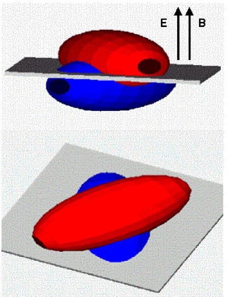
FIG. 1.: Cartoon depicting the momentum space effect of aligned chromoelectric and chromomagnetic fields on the momentum space distributions of quarks and antiquarks. We imagine that without the fields present, the two distributions can be pictured as overlaping ellipsoids which are elongated along the $p_{z}$-axis. The fields then alter these distributions to a state roughly like the one depicted in a very exaggerated manner in these two cartoons (the two cartoons show different views of the same situation). The plane drawn is the $p_{x}$-$p_{z}$ plane (assuming the fields are in the y-direction) and is included only to help to clarify the cartoon.

FIG. 2.: Illustration of the problem of observing parity violation when in each event the violation is equally likely to be right-handed or left-handed. Panel A shows the distribution of $T_{zz}$ for simulated events with no parity violating fields. Panel B shows the same distribution with $\vec{B}\cdot\vec{E}>0$ for every event. For panel C, $\vec{B}\cdot\vec{E}$ is as likely greater than as less than zero in each event; this is expected to be the case if strong CP violation occurs. The difference between panels A and C then is simply in the width of the distribution, and this is the basic signal of parity violation (shown here in exaggeration) for which we are searching with the methods described here.

TABLE I.: Estimated number of central RHIC events needed to see a $3\sigma$ signal for the observable $T_{zz}$, as a function of ’bubble’ size and field strength in Model $I$ (assuming a STAR-like acceptance). The top two cases are those that we discuss in the text as the ’nominal’ cases for these parameters. A value for the top case in the Subevent method is not included because a sufficient number of simulation events have not been run.

Field Strength	$R_{dom}/R_{tot}$	Events Needed (Mixed Event)	Events Needed(Subevent)
1	1/5	10M
1	2/5	50K	30M
1	3/5	3K	350K
2	3/5	300	1.5K
3	3/5	100	200

TABLE II.: Results from the three different simulation models for the number of central RHIC events needed to observe a $3\sigma$ signal resulting from CP violation using the mixed-event method and ’nominal’ values for bubble size and field strength as described in the text. These results are assuming a detector with acceptance similar to that of STAR.

Model	Number of Events Needed
$I$	10M
$II$	200K
$III$	2M

REFERENCES

- [1] T. D. Lee and C. N. Yang, Phys. Rev. 104(1956) 254. C. S. Wu, et al., Phys. Rev. 105(1957) 1413.
- [2] J. H. Christenson et al., Phys. Rev. Lett. 13(1964)138.
- [3] Peccei, R. D., in CP violation, C. Jarlskog, ed. World Scientific (1989).
- [4] D. Kharzeev, R. D. Pisarski, and M. H. G. Tytgat, Phys. Rev. Lett. 81(1998)512.
- [5] P. D. Morley and I. A. Schmidt, Z. Phys. C 26 (1985)627.
- [6] D. Kharzeev and R. D. Pisarski, Phys. Rev. D 61(2000)111901.
- [7] M. Gyulassy, RBRC Memo, 1999. www-cunuke.phys.columbia.edu/people/gyulassy/RHIC/cp_twist.ps
- [8] K. Buckley, T. Fugleberg, and A. Zhitnitsky, Phys. Rev. Lett. 84 (2000)4814.
- [9] D. Ahrensmeier, R. Baier, and M. Dirks, Phys. Lett. B 484(2000) 58.
- [10] K. Buckley, T. Fugleberg, and A. Zhitnitsky, Phys. Rev. C 63 (2001)034602.
- [11] E. Witten, Nucl. Phys. B 233(1983)422.
- [12] J. Wess and B. Zumino, Phys. Lett. 37B(1971)95.
- [13] Robert G. Sachs. The Physics of Time Reversal. The University of Chicago Press (1987)
- [14] A. Chikanian and J. Sandweiss, ”Parity and Time Reversal Studies in STAR”, report 1999.
- [15] S. Voloshin, Phys. Rev. C 62(2000)044901.
- [16] X.N. Wang and M. Gyulassy, Phys. Rev. D 44(1991)3501.
- [17] K.H. Ackerman et al., Nucl. Phys. A661(1999)681.
- [18] S. Voloshin, V. Koch, and H.G. Ritter, Phys. Rev. C 60 (1999)024901.
- [19] S. J. Lindenbaum and R. Longacre, J. Phys. G 26(2000)937.
- [20] T. Ludlam et. al., 1985 RHIC Workshop (Brookhaven National Lab, April, 1985), ed. P. Haustein and C.L. Woody.
- [21] D. Kharzeev, private communication and 3/99 Riken BNL workshop. www.star.bnl.gov/STAR/html/parity_l/kharzeev-3-11-99.pdf .
- [22] K. H. Ackermann et. al., Phys. Rev. Lett. 86(2001)402.
- [23] D.L. Adams et al., Phys. Lett. B 264(1991)462.
- [24] M. Anselmino, M. Boglione, and F. Murgia, Phys. Lett. B 362 (1995)164.