Chiral dynamics in few–nucleon systems

Abstract

We report on recent progress achieved in calculating various few–nucleon low–energy observables from effective field theory. Our discussion includes scattering and bound states in the 2N, 3N and 4N systems and isospin violating effects in the 2N system. We also establish a link between the nucleon–nucleon potential derived in chiral effective field theory and various modern high–precision potentials.

1 Introduction

Chiral effective field theory (EFT) offers a systematic and controlled method to study the dynamics of few–nucleon systems. In the approach proposed by Weinberg Weinb1 ; Weinb2 , one starts from an effective Lagrangian for nucleon and pion fields as well as external sources, in harmony with chiral and gauge invariance. The effective nucleon–nucleon (NN) potential is constructed using a unitary transformation to avoid any energy-dependence and applying systematic power counting, as described in ref. EGM1 . To leading order, one has the one–pion exchange (OPE) together with two contact terms accompanied by low–energy constants (LECs). At next–to–leading order (NLO), renormalizations of the OPE, the leading two–pion exchange (TPE) diagrams and seven more contact operators appear. At NNLO, one has to include the subleading TPE with one insertion of dimension two pion–nucleon vertices (the corresponding coupling constants are denoted by $c_{1,3,4}$). The potential is then used in a properly regularized Lippmann–Schwinger equation (e.g. by a sharp or exponential momentum cut-off) to generate the bound and scattering states, as detailed in ref.EGM2 . The iteration of the potential leads to a non–perturbative treatment of the pion exchange which is of major importance to properly describe the NN tensor force. The nine LECs are to be determined from a fit to the low $np$ partial waves. Here, we discuss implications of the uncertainties in the values of the $c_{i}$’s to various properties of chiral forces. Apart from the already published NNLO potential with numerically large values of the $c_{i}$’s, taken from ref.Paul , we construct the NNLO* version with (numerically) reduced and fine tuned values of $c_{3}$, $c_{4}$. We also discuss physical mechanisms, which can explain such smaller values of these low–energy constants. In contrast to the NNLO version, the NNLO* chiral potential does not lead to deeply lying bound states. This makes it more suitable for many–body applications. Both versions reproduce $np$ phase shifts in most partial waves fairly well up to $E_{\rm lab}\sim 200$ MeV. In the same framework, one can also include charge symmetry breaking and charge dependence of the nuclear force by including the light quark mass difference and elecromagnetic corrections WME . This allows to predict differences between some phase shifts in $pp$ and $nn$ systems. The extension to three– and four–nucleon systems has also been started using the NLO potential ourPRL . At this order, no 3N forces (3NF) appear and one can make parameter–free predictions. We also present some first NNLO* results including only two–nucleon forces. We further show that the numerical values of the LECs can be understood on the basis of phenomenological one–boson–exchange (OBE) models EGME . We also extract these values from various modern high accuracy NN potentials and demonstrate their consistency and remarkable agreement with the values in the chiral effective field theory approach. This paves a way for estimating the low–energy constants of operators with more nucleon fields and/or external probes.

2 Few–nucleon forces in chiral EFT

Chiral EFT is a powerful tool, which allows to calculate low–energy observables performing an expansion in powers of the low–energy scale $Q$ associated with momenta of external particles. The pion mass $M_{\pi}$ is treated on the same footing as $Q$. To select the relevant diagrams contributing to the S–matrix at a certain order, one makes use of power counting. This consists of a set of rules to calculate the power $\nu$ of the low–energy scale $Q$ for any given diagram. The precise meaning of the power counting scheme depends on the system one is investigating. In what follows, we will concentrate on various low–energy processes between few (2, 3 and 4) nucleons. The essential complication in that case compared to pion–pion or pion–nucleon scattering is given by the fact, that the nucleon–nucleon interaction is nonperturbative even at very low energies. To deal with this problem Weinberg proposed to use time–dependent (“old–fashioned”) perturbation theory instead of the covariant one. The expansion of the S–matrix, obtained using this formalism, has the form of a Lippmann–Schwinger equation with an effective potential, defined as the sum of all diagrams without pure nucleonic intermediate states. Such states would lead in ”old–fashioned” perturbation theory to energy denominators, which are by a factor of $Q/m$ smaller than those from the states with pions and which destroy the power counting. Here and below, $m$ denotes the nucleon mass. The effective potential is free from such small energy denominators and can, in principle, be calculated perturbatively to any given precision. This strategy has been followed in the pioneering work by Ordóñez et al. ord . The effective NN Hamiltonian derived in this formalism possesses some unpleasant properties: it depends, in general, explicitly on the energy of incoming nucleons and is not Hermitean. This complicates its application to few–nucleon systems. In order to avoid these problems we construct an effective NN Hamiltonian using the method of unitary transformation (projection formalism), as described in ref. EGM1 . For that we modify Weinberg’s power counting in an appropriate way. All details are given in EGM1 . In what follows, we will show the qualitative and the quantitative results for the effective potential in the first few orders of the chiral expansion.

Figure 1: First orders in the chiral expansion for few–nucleon forces, as explained in the text. Solid (dashed) lines denote nucleons (pions). The heavy dots, filled square and filled diamond denote the $\Delta_{i}=1$, $\Delta_{i}=2$ and $\Delta_{i}=4$ vertices, respectively.

Let us begin with the power counting. As pointed out above, any (time–ordered) diagram ${\cal T}$ contributing to the few–nucleon scattering process scales as:

$${\cal T}\sim\left(Q/\Lambda_{\chi}\right)^{\nu}~{},$$ (1)

where $\Lambda_{\chi}\sim 1$ GeV is the typical scale of chiral symmetry breaking. For any diagram with $E_{n}$ nucleons, $L$ loops and $V_{i}$ vertices of type $i$ one has (we only consider connected diagrams):

$$\nu=-4+2E_{n}+2L+\sum_{i}V_{i}\Delta_{i}\;,$$ (2)

where each vertex carries the index $\Delta_{i}$ (also called chiral dimension) given by

$$\Delta_{i}=d_{i}+\frac{1}{2}n_{i}-2\;.$$ (3)

Here, $n_{i}$ is the number of nucleon field operators and $d_{i}$ is the number of derivatives (or pion mass insertions). Due to spontaneously broken chiral symmetry, the index $\Delta_{i}$ cannot be negative. As a consequence, the power $\nu$ of the low–energy scale $Q$ is bounded from below and a systematic and perturbative expansion for an effective Hamiltonian becomes possible. Let us now concentrate on the first few orders in the chiral expansion.

• LO ($\nu=0$) The power $\nu$ of the low–energy scale $Q$ takes its minimal value $\nu=0$ for tree diagrams with two nucleons ($E_{n}=2$) and with all interactions of dimension $\Delta_{i}=0$. Thus, the potential at LO is given by OPE and contact interactions without derivatives, see fig. 1. There are no 3N and 4N forces at LO.

• NLO ($\nu=2$) The first corrections to the 2N potential are given by tree diagrams with one insertion of $\Delta_{i}=2$ interaction (seven independent contact interactions with two derivatives) as well as by one–loop graphs with all leading vertices (leading chiral TPE). Nominally, one has also three–nucleon forces given by tree diagrams with $\Delta_{i}=0$ vertices. In the projection formalism it turnes out, that the total contribution from those diagrams vanishes. If “old–fashioned” perturbation theory is used to derive the effective potential, the contribution of the corresponding 3N force cancels against energy dependent part of once iterated LO potential Weinb1 ; kolck2 . Thus, there are no 3N and 4N forces at this order.

• N²LO ($\nu=3$) The N²LO 2N potential is given by the subleading chiral TPE with one $\pi\pi NN$ vertex of dimension $\Delta_{i}=1$. There are three independent structures in the Lagrangian, which contribute to NN scattering. The corresponding LECs are denoted by $c_{1,3,4}$ BKMrev . Note that no additional contact interactions appear at that order. There are first nonvanishing three–nucleon forces.

• N³LO ($\nu=4$) The chiral potential at this order has not yet been worked out completly. Some calculations were performed by Kaiser Kaiser . At this order one has first 4N forces as well as a large number of various 3N and 2N interactions (including two– and three–pion exchange graphs).

Note that one can easily write down the contributions to the effective potential within “old–fashioned” perturbation theory, which correspond to the diagrams shown in fig. 1. The contributions in the projection formalism are, however, not easily recoverable without knowledge of the explicit operator expressions. The diagrams of fig. 1 should therefore serve only as a guidance. For the precise numerical prefactors as well as the energy denominators corresponding to the graphs shown the reader is refered to ref.EGM1 . We would like to point out one of the most important qualitative findings of chiral EFT applied to few–nucleon systems Weinb2 , kolck2 . As shown in fig. 1, the chiral power counting eq. (2) suggests, that 3N forces are weaker than 2N ones, 4N forces are weaker than 3N ones etc..

3 Applications

In what follows, we will discuss application of the described formalism to 2N, 3N and 4N systems, consider some isospin violating effects and establish connection between chiral NN forces and OBE models.

3.1 Two nucleons

Let us now concentrate on the parameters entering the NN potential. The two unknown LECs at LO associated with the contact interactions without derivatives have to be fixed by a fit to S–wave phase shifts at low energies. The leading chiral TPE at NLO is parameter–free. At this order one has in addition seven unknown LECs, which corresponds to contact terms with two derivatives. Those constants as well as the two LO LECs are fixed from fit to phase shifts in S– and P–waves and to the mixing angle $\epsilon_{1}$. Thus, one has nine unknown constants at this order, see ref. EGM2 for more details. As already stressed before, the subleading TPE at NNLO depends on the LECs $c_{1,3,4}$, which corresponds to $\pi\pi NN$ vertices of dimension $\Delta_{i}=1$. Precise numerical values of these constants are crucial for some properties of the effective potential. Clearly, the subleading $\pi\pi NN$ verices represent an important link between NN scattering and other processes, such as $\pi N$ scattering. Ideally, one would like, therefore, to take their values from the analysis of the $\pi N$ system. Various calculations for $\pi N$ scattering have been performed and are published. From the $Q^{2}$ analyses BKM95 one gets: $c_{1}=-0.64\,,c_{3}=-3.90\,,c_{4}=2.25\;$. Here all values are given in GeV^-1. From various $Q^{3}$ calculations BKM95 , BKM97 , Moi98 , FMS99 , Paul one gets the following bands for the $c_{i}$’s:

$$c_{1}=-0.81\ldots-1.53\,,\quad\quad c_{3}=-4.70\ldots-6.19\,,\quad\quad c_{4}=3.25\ldots 4.12\,.$$ (4)

Recently, the results from the $Q^{4}$ analysis have become available FM00 . At this order the S–matrix is sensitive to 14 LECs (including $c_{1,3,4}$), which have been fixed from a fit to $\pi N$ phase shifts. It turnes out that different available phase shift analyses (PSA) from refs. Koch86 , Mat97 and SAID lead to sizable variation in the actual values of the LECs. In particular, the dimension two LECs acquire a quark mass renormalization. The corresponding shifts are proportional to $M_{\pi}^{2}$. The renormalized $c_{i}$’s are denoted by $\tilde{c}_{i}$. A typical fit based on the phases of ref.  Mat97 leads to:

$$\tilde{c}_{1}=-0.27\pm 0.01\,,\quad\quad\tilde{c}_{3}=-1.44\pm 0.03\,,\quad\quad\tilde{c}_{4}=3.53\pm 0.08\;.$$ (5)

However, using the older Karlsruhe or the VPI phases as input, one finds sizeable variation in the $\tilde{c}_{i}$. Alternatively, one can also keep the $c_{i}$ at their third order values and fit the fourth order corrections separately, see FM00 . Due to the fitting range chosen and uncertainties in the isoscalar amplitudes, these pieces are not very well determined. In principle, these fits could be improved by including the scattering lengths determined from pionic hydrogen/deuterium. It should also be stressed that numbers consistent with the band given in eq.(4) have been obtained in BL using IR regularized baryon chiral perturbation theory and dispersion relations. Comparable values of $c_{1,3,4}$ have also been obtained by Rentmeester et al. from analysis of the $pp$ data Rent . A few comments are in order. First of all, the numerical values of some of the $c_{i}$’s appear to be quite large. Indeed, from the naive dimensional analysis one would expect, for example, $c_{3}$ to scale like:

$$c_{3}\sim{\ell}/2m\sim{\ell}/2\Lambda_{\chi}\,,$$ (6)

where ${\ell}$ is some number of order one. Taking the value $c_{3}=-4.70$ from ref. Paul and $\Lambda=M_{\rho}=770$ MeV we end up with ${\ell}\sim-7.5$ . Such a large value can be partially explained by the fact that the $c_{3,4}$ are to a large extent saturated by the $\Delta$–excitation. This implies that the different and smaller scale, namely $m_{\Delta}-m\sim 293$ MeV, enters the values of these constants, see BKM97 . More work on pion-nucleon scattering (dispersive versus chiral representation), new dispersive analyses and more precise low-energy data are needed to pin down these LECs to the precision required here. Applied to NN scattering, the large numerical values of the $c_{i}$’s might lead to a slow convergence of the low–momentum expansion. Another consequence of the large $c_{i}$’s for the NN system is the appearance of spurious deeply bound states in low partial waves, which can be traced back to a very strong attractive central potential related to the subleading TPE. The spurious states do not influence low–energy observables, as explained in EGM2 . The important consequence is, however, that strong 3NF are needed. Note that despite this very different scenario from what is expected in conventional nuclear physics (small 3N forces), the individual contributions of the 2N and 3N forces to observables can, in principle, not be observed experimentally. Since the actual values of the $c_{i}$’s may possibly change in future analyses of the $\pi N$ system (higher orders, more precise PSA, etc.), we constructed the NNLO* version of the NN potential, in which we basically subtracted the $\Delta$–contributions to these LECs and allowed for some fine tuning. This results in numerically reduced values of the $c_{3,4}$: $c_{3}=-1.15\,$GeV^-1, $c_{4}=1.20\,$GeV^-1. As a consequence, no unphysical deeply bound states appear This is partially motivated by the fact that the $\Delta$ is not included as an explicit degree of freedom in existing OBE models leading to very good quantitative description of observables. Some steps along a deeper understanding of the surprisingly modest role of the $\Delta$ in the NN system within boson exchange models have been undertaken in the framework of the Bonn potential HME ; Juelpirho . It was pointed out that there are strong cancellations between the TPE, whose dominant part is given by diagrams with intermediate $\Delta$–excitations, with the $\pi\rho$–exchange. Such a cancellation should ultimately also be observed in EFT studies, but that would require a consistent power counting scheme including vector mesons. Such a scheme has not yet been constructed. Let us finally point out that we do not know at the moment, whether the NNLO or NNLO* versions are closer to reality. Further studies of different processes as well as going to higher orders in the NN system may shed some light on to this question. In what follows, we will use the NNLO* potential in our 3N and 4N calculations as well as for comparison with conventional models. We are now in the position to give quantitative results. In fig.2 we show the two $np$ S-wave phase shift ${}^{1}S_{0}$ and ${}^{3}S_{1}$ and the ${}^{3}S_{1}-^{3}D_{1}$ mixing parameter at NLO (left panel) and NNLO* (right panel) in comparison to the Nijmegen PSA. To regularize the LS equation, we have used an exponential regulator $f_{R}(\vec{p})=\exp(-p^{4}/\Lambda^{4}$) (for details, see EGM2 ). The two lines correspond to cut-offs $\Lambda=500$ and $600$ MeV. We note that the description of the phases improves when going from NLO to NNLO* and that also the cut-off dependence gets weaker (especially at low energies). This is to be expected from a converging EFT and we emphasize again that this is not the result of an increasing number of free parameters. For the other phase shifts and a more detailed discussion, see EGMtoappear .

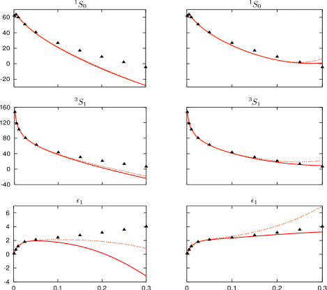
Figure 2: Phase shifts at NLO (left panel) and NNLO* (right panel) versus the lab energy (in GeV) in comparison to the Nijmegen PSA. The solid (dashed) line corresponds to $\Lambda=500$ ($\Lambda=600$) MeV.

3.2 Isospin violation

It is well known that charge symmetry (CS) and charge independence (CI) of the nuclear force are violated. In the Standard Model, these are manifestations of isospin violation (IV). There are two distinct sources of IV. In pure QCD, the light quark mass difference $m_{u}-m_{d}$ is the only source of IV. This can easily be incorporated in the EFT by means of an external scalar source. Since the charges of the quarks are also different, there is an additional electromagnetic contribution to IV. The electromagnetic effects due to hard photons are represented by local contact interactions. Soft photons appear in loop diagrams and also generate the long–range Coulomb potential. In WME , these effects have been studied in some detail, extending earlier work of van Kolck and collaborators kolck3 ; KFG . The power counting is extended to include the electromagnetic interactions with the fine structure constant $\alpha$ serving as the additional small parameter. With this, one can construct the various contributions to the NN potential. It consists of two distinct pieces, the strong (nuclear) potential including isospin violating effects and the Coulomb potential. The nuclear potential consists of one– and two–pion exchange graphs (with different pion and nucleon masses), $\pi\gamma$ exchange diagrams and a set of local four–nucleon operators (some of which are isospin symmetric, some depend on the quark charges and some on the quark mass difference). Since the nuclear effective potential is naturally formulated in momentum space, the matching procedure developed in ref.VP to incorporate the correct asymptotical Coulomb states was employed in WME . More precisely, the classification of the IV contributions to the NN potential is a as follows: To leading order one has to consider the pion mass difference in the OPE and the Coulomb potential. NLO IV corrections stem from the pion mass difference in the TPE, from $\pi\gamma$ exchange and from two four-nucleon contact interactions with no derivatives which have the generic structure:

$${\cal O}_{\rm CSB}\sim(N^{\dagger}\tau_{3}N)(N^{\dagger}N),\quad{\cal O}_{\rm CIB}\sim(N^{\dagger}\tau_{3}N)^{2}~{}.$$ (7)

These operators parameterize non-pionic CS breaking and CI breaking effects. The low–energy constants accompanying the contact interactions and the cut–off $\Lambda$ were determined in WME by a simultaneous best fit to the S– and P–waves of the Nijmegen phase shift analysis in the $np$ and the $pp$ systems for laboratory energies below 50 MeV. This allows to predict these partial waves at higher energies and all higher partial waves. Most physical observables come out independent of the sharp cut–off for $\Lambda$ between 300 and 500 MeV. The upper limit on this range is determined by the $pp$ interactions.

Figure 3: Phase shift difference $\delta_{\rm pp}-\delta_{\rm np}$ for the ${}^{3}P_{0}$ and ${}^{3}P_{2}$ partial waves in comparison to the Nijmegen PSA (dashed lines) and results from the CD-Bonn potential (filled circles).

In fig.3, we show the predictions for two P-waves in comparison to the Nijmegen PSA and the CD-Bonn potential. The range expansion for the $np$ and the $pp$ system was also studied in WME . For the range of cut–offs, the $pp$ scattering length varies modestly with $\Lambda$ due to the scheme–dependent separation of the nuclear and the Coulomb part, $|\delta a_{pp}/a_{pp}|\simeq 0.6~{}{\rm fm}/17~{}{\rm fm}\simeq 3\%$. This shows that the arbitrariness in separating the Coulomb and the nuclear part to $a_{pp}$ is strongly reduced within EFT because only a certain range of cut-offs allows to simultaneously describe $np$ and $pp$ scattering. Finally, it is worth to stress that CSB is largely driven by a contact interaction. The corresponding LEC can be understood to some extent in terms of $\rho-\omega$ mixing, see KFG .

3.3 Three and four nucleons

The NLO $np$ potential was applied to systems of three and four nucleons in ourPRL . At this order, one has no 3NF and thus obtains parameter–free predictions. One also gets a first indication about the theoretical accuracy of this approach. Consider first the binding energy. For changing the cut–off between 540 and 600 MeV, the ³H and ⁴He binding energies vary between $-7.55\ldots-8.28$ and $-24.0\ldots-28.1$ MeV, respectively, showing the level of accuracy of the NLO approximation for these observables. As discussed in detail in ourPRL , the chiral predictions for most observables like the differential cross section or the tensor analyzing powers $T_{ij}$ for elastic $nd$ scattering as well as break-up observables are in agreement with what is found for high precision potentials like CD-Bonn. One also observes a clear improvement in the analyzing power $A_{y}$ for low and moderate energies, compare the left and the right panels in fig.4. The cut-off dependence for the canonical range of $\Lambda$ is moderate, as indicated by the band in fig.4. These calculations have now been extended to NNLO, more precisely, using the NNLO* potential and neglecting all 3NFs, which appear at that order. For a detailed discussion of the results we refer to EGMtoappear . Here, we only remark that the cut-off sensitivity of the 3N and 4N binding energies is sizeably reduced at NNLO*, one finds e.g. $-29.96\ldots-27.87$ MeV for $E_{B}(^{4}{\rm He})$ for even extended cut–off range between 500 and 600 MeV (the overbinding is partly due to the fact that only an $np$ force is used). Also, the description of $A_{y}$ at 3 and 10 MeV is worse than at NLO, but it is still somewhat better than for the high-precision potentials and, more importantly, the cut-off dependence is much weaker as compared to NLO. Another crucial observation is that at NNLO* we are able to go to much higher energies than at NLO: our NNLO* prediction for $A_{y}$ at 65 MeV is in excellent agreemnet with the data. Of course, final conclusions can only be drawn when the 3NFs have been included. Work along these lines is underway. For some first steps in this direction see refhueber .

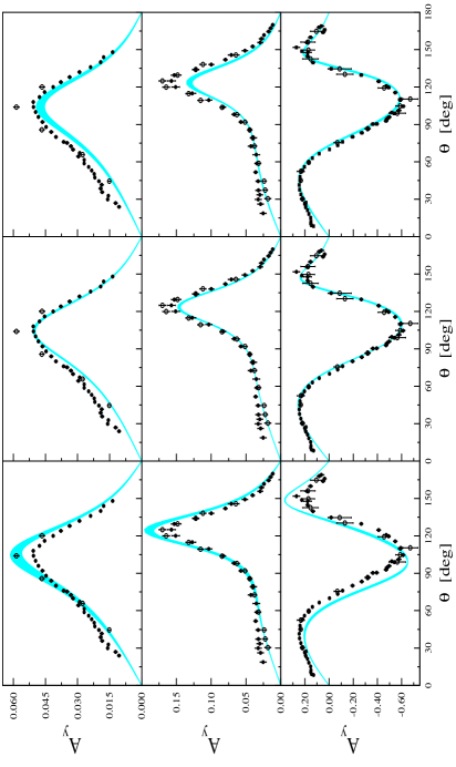
Figure 4: Analyzing power $A_{y}$ for elastic $nd$ scattering, for $E_{\rm lab}=3,10,65\,$MeV (top to bottom). Results at NLO (left panel) and NNLO* (middle panel). The band corresponds to the range $\Lambda=500$ to $600$ MeV. Results based on the high-precision potentials (CD-Bonn, AV-18, Nijm-93, Nijm-I,II) are shown in the right panel. Here the band refers to the uncertainty using the various potentials.

3.4 Connection to “realistic” potentials

Finally, we wish to provide a bridge between the EFT and traditional nuclear physics approaches. In the latter case, one constructs (semi)phenomenological potentials such that one can describe the NN data very precisely. One particular class are the boson exchange potentials, which besides OPE have heavy meson exchanges ($\sigma$, $\rho$, $\omega,\ldots$) to generate the intermediate range attraction, short range repulsion and so on. In most modern high-precision potentials (which lead to fits with a $\chi^{2}/{\rm datum}\sim 1$) the short-distance physics is parametized in different ways, say by boundary conditions, r-space fit functions or partial wave dependent boson exchanges. In EGME it was demonstrated that existing one–boson–exchange (or more phenomenologically constructed) models of NN force allow to explain the LECs in the chiral EFT potential in terms of resonance parameters. To be specific, consider a heavy meson exchange graph in a generic OBE potential. In the limit of large meson masses $M_{R}$, keeping the ratio of coupling constant $g$ to mass fixed, one can interpret such exchange diagrams as a sum of local operators with increasing number of derivatives (momentum insertions). In a highly symbolic relativistic notation, this reads,

$$(\bar{N}P_{i}N)\left({g^{2}\,\delta^{ij}\over M_{R}^{2}-t}\right)(\bar{N}P_{j}N)=\left({g^{2}\over M_{R}^{2}}\right)(\bar{N}P_{i}N)(\bar{N}P^{i}N)+\left({g^{2}\,t\over M_{R}^{4}}\right)(\bar{N}P_{i}N)(\bar{N}P^{i}N)+\dots~{},$$ (8)

where the $P_{i}$ are projectors on the appropriate quantum numbers for a given meson exchange (including also Dirac matrices if needed). Clearly, it is easy to express the dimension zero and two LECs, corresponding to the two terms of the r.h.s. of eq.(8), in terms of meson masses, coupling constants (and form factor scales, if required by the model). In the chiral EFT, one has to expand the TPE in a similar way and adjust its contribution to the various LECs accordingly. One can also repeat this procedure for the high-precision potentials, this has to be done numerically for the various partial waves. In fig.5 we show a comparison between the 4 S- and the 5 P-wave LECs obtained at NLO (leftmost bands) and NNLO* (central bands) and extracted from various OBE and high-precision potentials (see the inset in the figure). The agreement is rather stunning since one would have expected higher dimension operators to play a more prominent role in the phenomenological potentials (related e.g. to the cut-off sensitivity of the $\pi N$ form factor like in the Bonn potential). Note also that the theoretical uncertainties determined in EFT are a) small compared to their average values and b) are smaller than the band spanned by the potential models (even if one only includes the high–precision ones). Note that the comparison has been performed for the partial wave projected set of coupling constants.

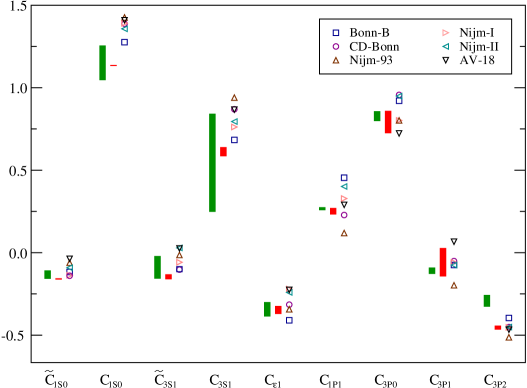
Figure 5: LECs from phenomenological models and chiral EFT. The leftmost band refers to NLO (the length reflects the variation with the cut-off), the middle bar is NNLO*, and the symbols correspond to the indicated potentials (see inset).

Let us now discuss the important issue of naturalness of the various LECs related to contact interactions. For that is turns out to be more appropriate to work directly with the coupling constants $C_{S}$, $C_{T}$, $C_{1\ldots 7}$, which enter the chiral Lagrangian, see EGME . Here, the constants $C_{S}$ and $C_{T}$ correspond to operators without derivatives, whereas the remaining ones to contact terms with two derivatives. Dimensional arguments suggest the following scaling properties of these LECs: $C_{C,S}\sim{l_{S,C}/(f_{\pi}^{2})}\;$, $C_{1\ldots 7}\sim{l_{1\ldots 7}/(f_{\pi}^{2}\,\Lambda_{\chi}^{2})}$, where the $l$’s are some numbers of order one. These scaling properties of the LECs are crucial for the convergence of the low–momentum expansion. Note that one has to take into account numerical prefactors which accompany the various terms of the Lagrangian, see ref. EGME for more details. Taking $\Lambda_{\chi}=1$ GeV it turnes out that the values of the $l$’s fluctuate between 0.3 and 3.5, i.e. the values found for these LECs are indeed natural, with the notable exception of $f_{\pi}^{2}\,C_{T}$, which is much smaller than one: $f_{\pi}^{2}C_{T}=-0.002\ldots 0.147$ at NLO and $f_{\pi}^{2}C_{T}=0.002\ldots 0.040$ at NNLO*. These unnaturally small numbers can be traced back to the SU(4) symmetry of the NN interaction, proposed about 65 years ago by Wigner Wigner . For the recent discussion on that subject within the EFT approach see ref.  MSW .

4 Summary and outlook

Despite the original scepticism by its creator Weinb2 , chiral effective field theory not only offers qualitative but also quantitative insight into the dynamics of few-nucleon systems, as should have become clear from the discussed topics. In addition, it is the only framework at present in which one can address the question of the size of three (four) nucleon forces in a truely systematic manner. It is therefore evident that a vast effort has to be undertaken to pin down the chiral 3NF and apply it not only to few- but also many-body systems. Exciting times are ahead of us.

5 Acknowledgments

E.E. thanks the organizers for the invitation and support.

References

- (1) S. Weinberg, Phys. Lett. B251 (1990) 288.
- (2) S. Weinberg, Nucl. Phys. B363 (1991) 3.
- (3) E. Epelbaoum, W. Glöckle and U.-G. Meißner, Nucl. Phys. A637 (1998) 107.
- (4) E. Epelbaum, W. Glöckle and U.-G. Meißner, Nucl. Phys. A671 (2000) 295.
- (5) P. Büttiker, and U.-G. Meißner, Nucl. Phys. A668 (2000) 97.
- (6) M. Walzl, U.-G. Meißner, and E. Epelbaum, Nucl. Phys. A693 (2001) 663.
- (7) E. Epelbaum et al., Phys. Rev. Lett. 86 (2001) 4787.
- (8) E. Epelbaum, W. Glöckle, U.-G. Meißner, and Ch. Elster, nucl-th/0106007.
- (9) C. Ordóñez, L. Ray and U. van Kolck, Phys. Rev. C53 (1996) 2086.
- (10) U. van Kolck, Phys. Rev. C49 (1994) 2932.
- (11) V. Bernard, N. Kaiser, and U.-G. Meißner, Int. J. Mod. Phys. E4 (1995) 193.
- (12) N. Kaiser, Phys. Rev. C61 (2000) 014003; C62 (2000) 024001; C63 (2001) 044010; nucl-th/0107064.
- (13) V. Bernard, N. Kaiser, and U.-G. Meißner, Nucl. Phys. B457 (1995) 147.
- (14) V. Bernard, N. Kaiser, and U.-G. Meißner, Nucl. Phys. A615 (1997) 483.
- (15) M. Mojžiš, Eur. Phys. J. C2 (1998) 181.
- (16) N. Fettes, U.-G. Meißner, and S. Steininger, Phys. Lett. B640 (1998) 199.
- (17) N. Fettes, and U.-G. Meißner, Nucl. Phys. A676 (2000) 311.
- (18) R. Koch, Nucl. Phys. 448 (1986) 707.
- (19) E. Matsinos, Phys. Rev. C56 (1997) 3014.
- (20) SAID on–line program, R.A. Arndt et al., see website http://gwdac.phys.gwu.edu/.
- (21) M.C.M. Rentmeester, R.G.E. Timmermans, J.L. Friar, and J.J. de Swart, Phys. Rev. Lett. 82 (1999) 4992.
- (22) E. Epelbaum et al., in preparation.
- (23) T. Becher and H. Leutwyler, JHEP 0106 (2001) 017.
- (24) R. Machleidt, K. Holinde, and Ch. Elster, Phys. Rep. 149 (1987) 1.
- (25) G. Janssen, K. Holinde, and J. Speth, Phys. Rev. C54 (1996) 2218.
- (26) U. van Kolck, Few-Body Systems Suppl. 9 1995 444
- (27) U. van Kolck, J.L. Friar and T. Goldman, Phys. Lett. B371 (1996) 169.
- (28) C.M. Vincent and S.C. Phatak, Phys. Rev. C10 (1974) 391.
- (29) D. Hüber et al., Few–Body Syst. 30 (2001) 95.
- (30) E. Wigner, Phys. Rev. 51 (1937) 106, 51 (1937) 947, 56 (1939) 519.
- (31) T. Mehen, I.W. Stewart, and M.B. Wise, Phys. Rev. Lett. 83 (1999) 931.