Electron helicity-dependence

in $(e,e^{\prime}p)$ reactions with polarized nuclei

and the fifth response function

J.E. Amaro¹ and T.W. Donnelly²

¹ Departamento de Física Moderna, Universidad de Granada, Granada 18071, Spain

² Center for Theoretical Physics, Laboratory for Nuclear Science and Dept. of Physics,
Massachusetts Institute of Technology, Cambridge, MA 02139, U.S.A.

 

Abstract

The cross section for electron-induced proton knockout reactions with polarized beam and target is computed in a DWIA model. The analysis is focused on the electron helicity-dependent (HD) piece of the cross section. For the case of in-plane emission a new symmetry is found in the HD cross section, which takes opposite values for specific opposing pairs of nuclear orientations, explaining why the fifth response (involving polarized electrons, but unpolarized nuclei) is zero for this choice of kinematics. Even when this symmetry breaks down in the case of nucleon emission out of the scattering plane, it is shown that it is still present in the separate response functions. A physical explanation of these results is presented using a semi-classical model of the reaction based on the PWIA and on the concept of a nucleon orbit with its implied expectation values of position and spin.

 

PACS: 25.30.Fj; 24.10.Eq; 24.70.+s; 29.27.Hj

Keywords: electromagnetic nucleon knockout; polarized beam and target; final state interactions; structure response functions

MIT/CTP#3188 September 2001

1 Introduction

In this work we continue our systematic investigation of spin observables in $\vec{A}(\vec{e},e^{\prime}p)B$ reactions initiated in [1, 2]. Relying on the general formalism for exclusive reactions [3] we particularized in [1] to nucleon knock-out, performed an explicit multipole expansion of the response functions involved and developed a DWIA model of the reaction, including relativistic corrections [4]. This was applied in an analysis of the full set of multipoles or reduced response functions (defined to be independent of the polarization angles) that can be extracted in studies of such reactions. The emphasis there was placed on studies of the sensitivity of the predictions to variations in the final-state interactions (FSI) and to inclusion of relativistic contributions to the electromagnetic current. The results found showed that these have very different impacts on the various response functions, which implies in the end that the importance of the specifics of the reaction mechanisms underlying the cross section strongly depends on the choice of polarization angles. The possibilities opened by this sensitivity to interesting physical effects underscores the relevance of future research in intermediate-energy electro-nuclear physics with polarized targets.

Specifically, in [2] we computed the quasi-free $(e,e^{\prime}p)$ cross section for unpolarized electrons and proton knock-out from the $1d_{3/2}$ shell of polarized ³⁹K leaving the residual ³⁸Ar in its ground state. The analysis of the results found there as functions of the nuclear polarization angles revealed that the nuclear transparency indeed depends strongly on the polarization direction, and that the FSI effects can be maximized or minimized by just flipping the nuclear orientation. Some particular polarization directions were found for which the FSI are practically negligible (and thus a PWIA treatment is adequate in these cases) and others for which the FSI even produce an enhancement of the cross section. In conventional $(e,e^{\prime}p)$ studies with unpolarized nuclei an average over all directions is involved, this behavior is lost and the usual reduction from the PWIA predictions, due mainly to the imaginary part of the optical potential, is recovered.

A physical explanation of the results found in [2] was also provided, based on the PWIA and on the semi-classical concept of a nucleon orbit. When the nucleus is polarized, the proton orbit is oriented in a well-defined direction, and for a given value of the missing momentum ${\bf p}$, the proton can be localized within its orbit (characterized by the expectation value of its position in the semi-classical model). In this picture of the reaction, the electron interacts with the proton, transferring four-momentum $Q^{\mu}=(\omega,{\bf q})$ and the proton leaves the nucleus after crossing a certain amount of nuclear matter with some impact parameter. The strength of the FSI along the nucleon’s path before it leaves the nucleus enters in such a way that in cases where the proton is localized near the nuclear surface and “evaporates”, immediately leaving the nucleus, the FSI are found to be small, while in cases where it crosses the entire nucleus leaving it by the opposite side the FSI effects are large. One can also find cases where some components of the FSI are emphasized, for instance when the nucleon leaves the nucleus in a direction tangent to the surface, where it is found that the real and spin-orbit parts of the optical potential are the most important.

In the case of a purely absorptive optical potential, it was possible to fit the damping of the PWIA cross section (i.e., explain the nuclear transparency) by a simple exponential factor $e^{-\rho/\lambda}$, where $\rho$ is the computed length of the nucleon’s trajectory within the nucleus and the free parameter $\lambda$ is the nucleon mean free path. In the case of unpolarized nuclei other studies [5] have treated the damping of the $(e,e^{\prime}p)$ cross section in the lowest-order eikonal approximation or Glauber model for high proton energies. However, since an average over angular orientations is implied in this case, the position of the proton cannot be fixed.

The studies performed in [2] revealed the fine control over the FSI that can be attained by varying the nuclear polarization. Having at hand a very intuitive physical picture of the reaction where the reaction mechanism is expressed in geometrical terms is clearly expected to be very helpful as guidance in undertaking future experiments with polarized nuclei. We wish to emphasize the importance of performing this kind of theoretical analysis where the behavior of the observables is explored over the full range of polarization angles.

Very few studies exist in the literature involving exclusive reactions with polarized medium-weight nuclei; and most of these were made only in PWIA, as they were motivated by studies of selected aspects of the problem, specifically, of relativistic off-shell effects in the current [6] and of nuclear deformation effects in the context of the Nilsson model [7, 8]. The two previous analyses of the reaction that did include FSI in studies of polarization observables with medium-weight nuclei [9, 10] presented exploratory calculations of the cross section and/or response functions only for a few nuclear orientations (the three usual ones referred to the reaction plane: longitudinal, sideways and normal). In the case of electro-nuclear reactions with light polarized targets, the situation is different and very elaborated models already exist, such as that of [11] involving polarized deuterium.

In the work undertaken in [2] only the simplest case of unpolarized electrons scattered by polarized targets was considered. In the present study we consider the more complex situation in which the electron beam is also polarized and where a new observable, the electron helicity-dependent (HD) cross section, comes into play. Guided by our previous studies here we analyze the behavior of this observable for the full range of nuclear polarization angles and the impact of FSI within the DWIA model for the reaction. The results are interpreted in terms of the above-mentioned semi-classical model, which we shall see is still valid for this observable. However, new physical aspects of the reaction appear in this case: indeed not only is the expected position of the proton within the orbit relevant, but also its spin direction comes into play. In fact, it is well-known [4, 6, 7] that, while in PWIA the cross section for unpolarized electrons is proportional to the spin-scalar momentum distribution of the nuclear overlap function, the HD cross section is proportional to the spin-vector momentum distribution. As we shall see, this can be interpreted as the nucleon spin distribution in the orbit.

One of the goals of this paper is to provide an understanding of new symmetry properties of the spin observables with respect to certain class of rotations of the polarization vector that are seen in our results. The obvious symmetry of the observables under inversion of the polarization vector that appears in PWIA is broken when FSI are included. In contrast, the symmetry that we shall put in evidence is valid even in the presence of FSI, making it a more fundamental property of spin observables. This symmetry occurs between nuclear orientations that are located symmetrically with respect to the reaction plane. In the case of the HD cross section, it appears only for in-plane emission and produces a change of sign, hence averaging to zero in the case of unpolarized nuclei. For out-of-plane emission we shall show that the symmetry of the HD cross section breaks down, on the average yielding a non-null result for the fifth response function for unpolarized nuclei. The origin of this symmetry can be explained using the semi-classical model by exploring the symmetries of nucleon position and spin projections for different nuclear polarizations. In particular, we shall show that the symmetry is still present in the separate response functions even for out-of-plane emission. The reason why it is broken in this case for the HD cross section lies in the different behaviors found for the $T^{\prime}$ and $TL^{\prime}$ responses: while the $T^{\prime}$ changes sign, the $TL^{\prime}$ does not for out-of-plane emission. Since the HD cross section is a linear combinations of these two responses, the symmetry is not preserved in this observable.

Understanding the HD cross section has implications for the fifth response function. In [12] this observable was analyzed for proton knock-out from a $s_{1/2}$ shell assuming for the scattering state a plane wave with complex momentum. The results were interpreted in terms of the asymmetry between protons emitted above and below the scattering plane and the different paths followed by the nucleon on its way out of the nucleus. In this simple case no spin-orbit FSI effects were included; these were discussed in [13]. In the present work we consider proton knock-out from the $d_{3/2}$ shell of ³⁹K, which more typical, and the spin-orbit interaction is included in the FSI. Since in our model the spin direction of the proton is known as well as its orbital angular momentum, we are able to show geometrically how the symmetry of the HD cross section is preserved in the presence of a spin-orbit interaction.

After a short review of the DWIA model, in sect. 2 we show results for the HD cross section over the full range of polarization directions and for in-plane and out-of-plane proton emission, as well as for the HD response functions, to reveal the symmetry properties of these observables. In sect. 3 we focus on the semi-classical model description of the reaction and compute the expected values of position and spin of the initial proton at a fixed value of missing momentum for a full range of the polarization angles in order to explain the DWIA results in a geometrical picture, giving an analytical proof of the symmetry properties in the Appendix. In sect. 4 we summarize our conclusions.

2 The DWIA model and results for the helicity-dependent cross section

The general formalism for exclusive electron scattering with polarized beam and target can be found in [3]. In this section we summarize some of the results that are essential for our present discussions. See [1, 2] for further details of our model.

We consider an electron with four-momentum $K^{\mu}=(\epsilon_{e},{\bf k}_{e})$ and helicity $h$ which is scattered through an angle $\theta_{e}$ by a nucleus, transferring four-momentum $Q^{\mu}=(\omega,{\bf q})$. We assume the extreme relativistic limit for the electron $\epsilon_{e}\gg m_{e}$ and the plane-wave Born approximation for the electron scattering amplitude. We work in a coordinate system where the $x$-$z$ plane is the scattering plane, with the $z$-axis in the direction ${\bf q}$ and the $x$ axis defined by the transverse component of the electron momentum ${\bf k}_{e}$.

After the scattering, a proton with energy $E^{\prime}$ is detected in the direction ${\bf\hat{p}}^{\prime}=(\theta^{\prime},\phi^{\prime})$ in coincidence with the electron. In this work the momentum of the ejectile is determined assuming relativistic kinematics $E^{\prime}{}^{2}-{\bf p}^{\prime}{}^{2}=M^{2}$, where $M$ is the nucleon mass. We work in the lab. frame where the target nucleus is at rest in its ground state. We assume that it has total spin $J_{i}$ and is 100% polarized in the direction $\mbox{\boldmath$\Omega$}^{*}$ defined by the polar and azimuthal angles $\Omega^{*}=(\theta^{*},\phi^{*})$, measured in the above coordinate system:

$$|A(\Omega^{*})\rangle=|J_{i}J_{i}(\Omega^{*})\rangle.$$ (1)

The unobserved residual nucleus is assumed to be left in a discrete state $|B\rangle$ and we neglect its recoil. The corresponding coincidence cross section can be written as

$$\frac{d\sigma}{d\epsilon^{\prime}_{e}d\Omega^{\prime}_{e}d{\bf\hat{p}}^{\prime}}=\Sigma+h\Delta,$$ (2)

where $\Sigma$ is the cross section for unpolarized electrons

$$\Sigma=\sigma_{Mott}(v_{L}{\cal R}^{L}+v_{T}{\cal R}^{T}+v_{TL}{\cal R}^{TL}+v_{TT}{\cal R}^{TT})$$ (3)

and $\Delta$, the observable we are interested in here, is the helicity-dependent cross section, given by

$$\Delta=\sigma_{Mott}(v_{T^{\prime}}{\cal R}^{T^{\prime}}+v_{TL^{\prime}}{\cal R}^{TL^{\prime}}).$$ (4)

The quantities $v_{K}$ and $v_{K^{\prime}}$ are electron kinematical factors coming from the leptonic tensor [3]. The exclusive response functions ${\cal R}^{K}$, ${\cal R}^{K^{\prime}}$ are specific components of the hadronic tensor

$$W^{\mu\nu}=\sum_{m_{s},M_{B}}\langle{\bf p}^{\prime}m_{s},B|J^{\mu}({\bf q},\omega)|A\rangle^{*}\langle{\bf p}^{\prime}m_{s},B|J^{\nu}({\bf q},\omega)|A\rangle$$ (5)

containing the transition matrix elements of the nuclear electromagnetic current operator $J^{\mu}({\bf q},\omega)$. The final (unpolarized) state is defined by the asymptotic boundary condition of a nucleon with momentum ${\bf p}^{\prime}$ and spin projection $m_{s}$, together with a daughter nucleus $|B\rangle=|J_{B}M_{B}\rangle$. We sum over final, undetected magnetic quantum numbers.

The relevant response functions in this work are the helicity-dependent ones, defined by

$${\cal R}^{T^{\prime}} = i(W^{xy}-W^{yx})\equiv W^{T^{\prime}}$$ (6)

$${\cal R}^{TL^{\prime}} = i\sqrt{2}(W^{0y}-W^{y0})\equiv W^{TL^{\prime}}\sin\phi^{\prime}+\tilde{W}^{TL^{\prime}}\cos\phi^{\prime},$$ (7)

where we have extracted the explicit dependence on the azimuthal emission angle $\phi^{\prime}$. The response functions $W^{T^{\prime}}$, $W^{TL^{\prime}}$ and $\tilde{W}^{TL^{\prime}}$ depend on $q$, $\omega$, $\theta^{\prime}$, $\theta^{*}$ and $\Delta\phi\equiv\phi^{\prime}-\phi^{*}$. In this work we fix the values of the energy-momentum transfer around the quasielastic peak, $p^{\prime}\sim q$, where the impulse approximation used here is expected to to work well. We present results for the HD cross section $\Delta$ as a function of the missing momentum $p$, defined as ${\bf p}={\bf p}^{\prime}-{\bf q}$, for a range of values of the angles $\phi$, $\theta^{*}$ and $\Delta\phi$.

For the electromagnetic operators we consider a new expansion of the relativistic on-shell current in powers of ${\bf p}/M$, with ${\bf p}$ the initial nucleon momentum, eliminating the final momentum ${\bf p}^{\prime}$ using momentum conservation [14, 15]. This is a very convenient expansion for intermediate-to-high energy quasi-free processes where the initial nucleon is in a bound state (and therefore its momentum is small enough so that a first-order expansion works well), but the final momentum is large (comparable with $q$) and hence the traditional expansions in ${\bf p}^{\prime}/M$ are bound to fail. Under this expansion, the charge and transverse current operators in momentum space are given by

$$\rho({\bf p}^{\prime},{\bf p}) = \rho_{c}+i\rho_{so}(\cos\phi\sigma_{y}-\sin\phi\sigma_{x})\delta$$ (8)

$$J^{x}({\bf p}^{\prime},{\bf p}) = iJ_{m}\sigma_{y}+J_{c}\delta\cos\phi$$ (9)

$$J^{y}({\bf p}^{\prime},{\bf p}) = -iJ_{m}\sigma_{x}+J_{c}\delta\sin\phi,$$ (10)

where $\delta\equiv\eta\sin\theta$, $\eta=p/M$, and the angles $(\theta,\phi)$ define the direction of the initial momentum ${\bf p}$. Note the spin-dependence explicit in the Pauli matrices. Finally, using our previous work the coefficients $\rho_{c}$ (charge), $\rho_{so}$ (spin-orbit), $J_{m}$ (magnetization), and $J_{c}$ (convection) are given by

$$\rho_{c}=\frac{\kappa}{\sqrt{\tau}}G_{E}, \rho_{so}=\frac{2G_{M}-G_{E}}{\sqrt{1+\tau}}\frac{\kappa}{2},$$ (11)

$$J_{m}=\sqrt{\tau}G_{M}, J_{c}=\frac{\sqrt{\tau}}{\kappa}G_{E}.$$ (12)

Here, as in past work, we use the dimensionless variables $\kappa=q/2M$ and $\tau=(q^{2}-\omega^{2})/4M^{2}$, and $G_{E}$ and $G_{M}$ are the electric and magnetic form factors of the nucleon, respectively, for which we use the Galster parameterization [16].

The inclusive electromagnetic responses obtained in the present model for the current were tested against the relativistic Fermi gas model in [14], while in [17] our present DWIA model of unpolarized $(e,e^{\prime}p)$ reaction was compared with a fully-relativistic model for $|Q^{2}|=0.8$ (GeV/c)². In both cases for quasi-free kinematics the expansion procedure was shown to be robust.

Figure 1: Helicity-dependent cross section for in-plane emission, as a function of the missing momentum. The various panels correspond to different pairs of polarization angles $(\theta^{*},\Delta\phi)$. From up to down $\theta^{*}=0,45,90,135$ and 180^o; from left to right $\Delta\phi=0,45,90$ and 135^o. The meaning of the curves is the following: solid: DWIA; long-dashed: PWIA; dotted: DWIA but with just the imaginary part of the central optical potential; short-dashed: DWIA without spin-orbit contributions

Figure 2: Helicity-dependent cross section for in-plane emission, as a function of the missing momentum. The various panels correspond to different pairs of polarization angles $(\theta^{*},\Delta\phi)$. From up to down $\theta^{*}=45,90$ and 135^o; from left to right $\Delta\phi=180,225,270$ and 315^o. The meaning of the curves is the same as in Fig. 1.

In Figs. 1–4 we present results for the polarized HD cross section $\Delta$ for the reaction ³⁹K$(e,e^{\prime}p)\,^{38}$Ar_g.s. using a range of values of the angles $\phi$, $\theta^{*}$ and $\Delta\phi$. The reason for choosing the ³⁹K nucleus as target is twofold: first, being the nucleus of an alkali atom potassium is a good candidate to be polarized in experimental studies. Second, it is a medium-weight, closed-shell-minus-one nucleus and therefore the shell model is expected to be adequate for describing its nuclear structure in such a first exploratory study. Hence in our calculation the ³⁹K target is described as a proton hole in the $1d_{3/2}$ shell of the ⁴⁰Ca core, while the residual ³⁸Ar nucleus is described as two holes in the $1d_{3/2}$ shell, coupled to zero total angular momentum. Single-particle wave functions in a Woods-Saxon mean potential are used for the hole states, with parameters taken from [18]. The ejected proton wave function is obtained by solving the Schrödinger equation in an optical potential for which we employ the Schwandt parameterization [19]. More details on these aspects of our model are given in [1, 4].

In our calculations we have fixed the momentum transfer to $q=500$ MeV/c and the energy transfer to $\omega=133.5$ MeV, corresponding to the quasielastic peak, and the electron scattering angle to $\theta_{e}=30^{\rm o}$. For this choice of kinematics, the relevant leptonic factors take on the values $v_{T^{\prime}}=0.268$ and $v_{TL^{\prime}}=-0.176$. The kinetic energy of the ejected proton is 124.8 MeV, while its momentum is $p^{\prime}=499.7$ MeV/c.

In Fig. 1 the HD cross section $\Delta$ is shown for in-plane emission, $\phi=0^{\rm o}$ as a function of the missing momentum. The various panels correspond to different values of the polarization angles in multiples of 45^o; from up to down $\theta^{*}=0,45,90,135$ and 180^o; from left to right $\Delta\phi=0,45,90$ and 135^o. Note that in this case $\Delta\phi=-\phi^{*}$. Hence the polarization vectors in the 14 panels of Fig. 1 span a hemisphere. The other half of the sphere is presented in Fig. 2, where now $\theta^{*}=45,90,135^{\rm o}$ and $\Delta\phi=180,225,270,315^{\rm o}$. In each panel of Figs. 1–2 we show four curves corresponding to different treatments of the FSI. Solid lines correspond to the full optical potential, while long-dashed lines have been obtained without FSI, i.e., setting the optical potential equal to zero, and thus they coincide with the factorized PWIA. The dotted lines include only the imaginary part of the central optical potential and correspond to a purely absorptive model of the interaction. Finally, the short-dashed lines include as well the real part of the central optical potential. Neither the dotted nor the short-dashed lines include the spin-orbit part of the potential, which is only considered in the case of the solid lines. Looking at the various curves in the figures we get a feeling for the effects of the separate ingredients in the FSI for the full range of values of the polarization angles and find a wide variety of situations, going from large FSI, for instance for $\theta^{*}=45^{\rm o}$ and $\Delta\phi=0^{\rm o}$ (Fig. 1), to small FSI for $\theta^{*}=45^{\rm o}$ and $\Delta\phi=180^{\rm o}$ (Fig. 2). Such observations were explained in [2] for the case of the helicity-independent cross section $\Sigma$. They arise from the fact that the length of the nucleon’s path inside the nucleus is larger in the former case than in the latter. In the next section we will come back to the generalization to HD observables and again see how the semi-classical model may be used to shed light on the results.

Another point to emphasize here is the utility of having a plot of $\Delta$ for the full range of polarization angles as in Figs. 1–2 where we can study the symmetries of this observable by direct inspection. First we note that in going from one polarization to the opposite, the PWIA HD cross section changes its sign (long-dashed lines), but that this is not in general the case when the FSI are turned on. Compare, for instance the polarization $\theta^{*}=135^{\rm o}$, $\Delta\phi=45^{\rm o}$ (Fig. 1), with the opposite $\theta^{*}=45^{\rm o}$, $\Delta\phi=225^{\rm o}$ (Fig. 2). In the first case the FSI produce a 30% decrease of the strength (solid lines), while in the second the total FSI effects are negligible. We also note from Figs. 1–2 that only for opposing pairs having $\Delta\phi=0^{\rm o}$ or $180^{\rm o}$ does the HD cross section cancellation occur. Therefore the fact that the HD cross section for unpolarized nuclei is zero for $\phi=0^{\rm o}$ even in presence of FSI is not due to cancellations between opposite polarizations when taking the average over all angles.

Figure 3: The same as Fig. 1, but now for $\phi=90^{\rm o}$.

Figure 4: The same as Fig. 2, but now for $\phi=90^{\rm o}$.

Thus the following question arises: how do the cancellations occur in this observable if not for the behavior for opposite polarizations? The answer is again contained in the results of Figs. 1–2. Upon closer examination a new symmetry in the HD cross section becomes apparent. But this time it is exact even in presence of the FSI. In fact, if we take the origin of coordinates in the $(\theta,\Delta\phi)$ plane as the point $(90^{\rm o},90^{\rm o})$, represented in Fig. 1 as the panel in the third column and third row, then we see that $\Delta$ takes opposite values for polarization angles that are opposite with respect to this central point. Compare for instance the pairs of polarizations $(45^{\rm o},45^{\rm o})$ and $(135^{\rm o},135^{\rm o})$ or $(45^{\rm o},90^{\rm o})$ and $(135^{\rm o},90^{\rm o})$. The same kind of “nodal” symmetry is observed in Fig. 2 when we take as central point (or node) the panel $(\theta,\Delta\phi)=(90^{\rm o},270^{\rm o})$. In this way it appears that, when averaging over polarization angles, there will be cancellations between pairs of polarizations located symmetrically with respect to any of the two nodal panels and a zero value of $\Delta$ for unpolarized nuclei is expected. Note that the two nodal points correspond to polarization vectors that lie perpendicular to the reaction plane (or to the scattering plane in this case). Were the model calculations to be exact, we would expect to find that the HD cross section corresponding to the two nodes is exactly zero, as would be implied by the nodal symmetry. In fact, we see that it is very small in the two cases (of the order of $10^{-7}$–$10^{-6}$ in the units of the figures) — these values are within the numerical error of the multipole expansion in our calculation and hence they are compatible with zero. We have checked that the cited symmetry between various pairs of polarizations is always satisfied within this uncertainty and hence we conjecture that this nodal symmetry is an exact one. The same symmetry is also present in the helicity-independent cross section studied in [2], although this fact was not mentioned in that reference. The goal of the next section will be to explain its origin within the semi-classical model for the nucleon orbit using geometrical arguments.

Up to this point we have discussed only results for in-plane emission kinematics ($\phi=0^{\rm o}$). Now in Figs. 3–4 we show results for $\phi=90^{\rm o}$, where the reaction plane is perpendicular to the scattering one. The meaning of lines and of the various panels is the same as in Figs. 1–2, corresponding to angles $\theta^{*}$ and $\Delta\phi$ spanning all directions, but note that $\Delta\phi=90^{\rm o}-\phi^{*}$ is now minus the azimuthal polarization angle measured with respect to the reaction plane. Looking at the figures we note again that the PWIA results (long-dashed lines) are opposite for opposite polarizations and hence a result of zero for this observable is obtained, corresponding to the expected result for unpolarized nuclei when there are no FSI. In the presence of FSI the different paths followed by the proton for opposite polarizations are reflected again in different effects due to FSI. These are larger in general for the polarizations of Fig. 3 than for those of Fig. 4. A wide range of effects can be found, from situations where FSI produce a very large decrease of $\Delta$, for $(\theta^{*},\Delta\phi)=(90^{\rm o},45^{\rm o})$ (Fig. 3), even a change of sign for $(\theta^{*},\Delta\phi)=(135^{\rm o},45^{\rm o})$ (Fig. 3), passing cases with small effects for $(\theta^{*},\Delta\phi)=(135^{\rm o},315^{\rm o})$ (Fig. 4), to cases with a large increase due to FSI for $(\theta^{*},\Delta\phi)=(45^{\rm o},180^{\rm o})$ (Fig. 4).

A significant difference with respect to the $\phi=0^{\rm o}$ case is that the nodal symmetry with respect to the $(90^{\rm o},90^{\rm o})$ polarization is not found here. No other symmetry is observed and, as a consequence, there will be a non-zero result predicted for this observable if the nucleus is unpolarized, as expected, and this in the end will give rise to the fifth response function which can be measured by performing out-of-plane measurements with polarized electrons, but unpolarized nuclei.

Figure 5: Response function $W^{T^{\prime}}$ computed for a range of nuclear polarization angles $(\theta^{*},\Delta\phi)$. The meaning of the panels and curves is the same as in Fig. 1.

Figure 6: Response function $W^{T^{\prime}}$ computed for a range of nuclear polarization angles $(\theta^{*},\Delta\phi)$. The meaning of the panels and curves is the same as in Fig. 2.

Figure 7: Response function $\widetilde{W}^{TL^{\prime}}$ computed for a range of nuclear polarization angles $(\theta^{*},\Delta\phi)$. The meaning of the panels and curves is the same as in Fig. 1.

Figure 8: Response function $\widetilde{W}^{TL^{\prime}}$ computed for a range of nuclear polarization angles $(\theta^{*},\Delta\phi)$. The meaning of the panels and curves is the same as in Fig. 2.

Figure 9: Response function $W^{TL^{\prime}}$ computed for a range of nuclear polarization angles $(\theta^{*},\Delta\phi)$. The meaning of the panels and curves is the same as in Fig. 1.

Figure 10: Response function $\widetilde{W}^{TL^{\prime}}$ computed for a range of nuclear polarization angles $(\theta^{*},\Delta\phi)$. The meaning of the panels and curves is the same as in Fig. 2.

Deeper insight into the reasons why the nodal symmetry is broken for out-of-plane emission can be obtained if we study the behavior of the three response functions $W^{T^{\prime}}$, $W^{TL^{\prime}}$ and $\widetilde{W}^{TL^{\prime}}$ which contribute to $\Delta$ (see Eqs. (4,6,7)). These are shown in Figs. 5–10, again for the full set of values of polarization angles $(\theta^{*},\Delta\phi)$. Note that these responses do not depend on $\phi$. The $T^{\prime}$ response gives the same contribution to $\Delta$ for any value of $\phi$; on the other hand, in the case of the $TL^{\prime}$ response for $\phi=0^{\rm o}$ ($90^{\rm o}$) only the $\widetilde{W}^{TL^{\prime}}$ ($W^{TL^{\prime}}$) response contributes. Since for $\phi=0^{\rm o}$ we found nodal symmetry in the HD cross section, this symmetry should also be present in the two response functions which contribute to this observable, and in fact, we see in Figs. 5–6 and 7–8 that both $W^{T^{\prime}}$ and $\widetilde{W}^{TL^{\prime}}$ responses show this symmetry, changing sign for opposite polarizations with respect the nodal polarization angles $(\theta^{*},\Delta\phi)=(90^{\rm o},90^{\rm o})$. As a consequence, any linear combination of these two responses, such as the observable $\Delta$ for $\phi=0^{\rm o}$, will present the same nodal symmetry. Both responses are zero (within the numerical precision — see above) for the nodal polarizations, although the shape and sign of these two responses are in general different for other polarizations, and the effects of the FSI, especially those related to the real and spin-orbit parts of the optical potential, are also different.

Let us now examine the behavior of the $W^{TL^{\prime}}$ response shown in Figs. 9–10. As before we note that in PWIA this response changes sign for opposite polarizations, but that again this is no longer true when FSI are switched on, due to the different path traveled by nucleons in their way across the nucleus, this being larger for the polarizations of Fig. 9 than for those of Fig. 10. The most important difference for this response function as compared with the others is its behavior under polarization inversion with respect to the nodal polarization $(\theta^{*},\Delta\phi)=(90^{\rm o},90^{\rm o})$. This response still displays a symmetry even in presence of FSI, yet in this case there is no change of sign, i.e., this response is even under the nodal inversion of polarization, while the $W^{T^{\prime}}$ and $\widetilde{W}^{TL^{\prime}}$ responses are odd under it. This behavior explains why the fifth response function for unpolarized nuclei, obtained as an average of the results in Figs. 9–10, is not zero. However, the fact that the nodal symmetry persists in the three response functions, either of odd or even type, is an indication of the fundamental nature of this symmetry. In the case of the observable $\Delta$ for $\phi\neq 0^{\rm o}$, where responses with both kinds of symmetries appear, the nodal symmetry is broken, since the linear combination of odd and even functions does not display any symmetry.

In the last instance, the present results provide an alternative way to separate the $W^{T^{\prime}}$ from the ${W}^{TL^{\prime}}$ response in the HD cross section by performing a measurement with $\phi=90^{\rm o}$ for two different polarizations, $\Omega_{1}$ and $\Omega_{2}$, that are opposite with respect to the nodal polarization, and exploiting the odd and even symmetries of these responses. In fact, we just add and subtract the two values of $\Delta$ so obtained. From Eqs. (4,6,7) we have

$$\Delta(\Omega_{1})+\Delta(\Omega_{2}) = 2\sigma_{Mott}v_{TL^{\prime}}{W}^{TL^{\prime}}(\Omega_{1})$$ (13)

$$\Delta(\Omega_{1})-\Delta(\Omega_{2}) = 2\sigma_{Mott}v_{T^{\prime}}W^{T^{\prime}}(\Omega_{1}).$$ (14)

3 The semi-classical model and applications to the HD cross section

In this section we analyze the results of the previous section in terms of geometrical properties of the nucleon orbit for various nuclear polarizations and kinematics. In particular we shall see that the behavior observed for the response functions and HD cross section can be characterized by two parameters, namely, the expectation value of the nucleon position within the orbit, and the expectation value of its spin. One of our goals is to express in geometrical terms why the nodal symmetry (in both versions, even and odd) is happening.

The semi-classical model was introduced in [2] to explain the results of the $(e,e^{\prime}p)$ cross section $\Sigma$ for polarized nuclei. It was based on the PWIA, the 3-dimensional scalar momentum distribution and the expected position of the nucleon in its orbit. For the present applications of this picture to the observable $\Delta$ a new element has to be added to that model, namely the expected value of the nucleon’s spin.

3.1 PWIA responses

A characteristic of PWIA is that the exclusive responses (and hence the cross section) factorize as the product of a single-nucleon scalar or vector response times a scalar or vector momentum distribution

$${\cal R}^{K} = Mp^{\prime}w^{K}_{S}M_{S},\kern 28.45274ptK=L,T,TL,TT$$ (15)

$${\cal R}^{K^{\prime}} = Mp^{\prime}{\bf w}^{K^{\prime}}_{V}\cdot{\bf M}_{V},\kern 28.45274ptK^{\prime}=T^{\prime},TL^{\prime}$$ (16)

where $M_{S}({\bf p})$ and $M_{V}({\bf p})$ are respectively the scalar and vector momentum distributions. They are related to the partial momentum distribution spin matrix, $n({\bf p})$, for residual nucleus $|B\rangle$ through

$$n({\bf p})_{\mu\nu}\equiv\sum_{M_{B}}\langle B|a_{{\bf p}\nu}|A\rangle^{*}\langle B|a_{{\bf p}\mu}|A\rangle=\frac{1}{2}(M_{S}({\bf p})\delta_{\mu\nu}+{\bf M}_{V}({\bf p})\cdot\mbox{\boldmath$\sigma$}_{\mu\nu}).$$ (17)

The scalar $w_{S}^{K}$ and vector ${\bf w}_{V}^{K}$ single-nucleon responses are obtained from the corresponding single-nucleon current matrix [4]. For the situation of interest here with polarized electrons, only the vector responses contribute to the HD cross section. In the case of the single-nucleon current defined in Eqs. (8–10) the corresponding expressions are the following:

$${\bf w}_{V}^{T^{\prime}} = 2J_{c}J_{m}\delta(\cos\phi\,{\bf e}_{1}+\sin\phi\,{\bf e}_{2})-2J_{m}^{2}{\bf e}_{3}$$ (18)

$${\bf w}_{V}^{TL^{\prime}} = 2\sqrt{2}\rho_{c}J_{m}{\bf e}_{1}+2\sqrt{2}J_{c}\rho_{so}\delta^{2}\sin\phi(\cos\phi\,{\bf e}_{2}-\sin\phi\,{\bf e}_{1})$$ (19)

$$-2\sqrt{2}\rho_{so}J_{m}\delta\cos\phi\,{\bf e}_{3},$$

where the unit vectors ${\bf e}_{i}$ correspond to the coordinate system $O$ introduced above, with ${\bf e}_{3}$ in the ${\bf q}$-direction and ${\bf e}_{1}$ in the scattering plane (in the direction of ${\bf k}_{eT}$), while ${\bf e}_{2}$ is perpendicular to the scattering plane.

3.2 Vector momentum distribution and spin field

For this work we assume that the proton is knocked-out from the $1d_{3/2}$ shell of ³⁹K and the final nucleus ³⁸Ar is left in its ground state with total spin $J_{B}=0$. In the shell-model description of this process it was shown in [1] that the partial momentum distribution is proportional to the single-particle distribution of the $1d_{3/2}$ shell (for other values of the final nuclear spin or for knock-out from inner shells this is no longer true, although the following results can be generalized to include these more general cases). Hence, to simplify the following discussion, we shall assume that the initial proton is described by a single-particle wave function with quantum numbers $(lj)$, and that it is polarized in the direction $\mbox{\boldmath$\Omega$}^{*}$, i.e., it carries all of the nuclear polarization.

This wave function can be obtained from the corresponding wave function polarized in the $z$-direction (i.e., with magnetic number $m=j$) by applying the appropriate rotation operator $R$. In fact, we begin with a spatial rotation ${\cal R}$ that maps the $z$-axis onto the polarization direction $\Omega^{*}$. The rotated basis, denoted $O^{*}=({\bf e}^{*}_{1},{\bf e}^{*}_{2},{\bf e}^{*}_{3})$, is defined by

$${\bf e}^{*}_{i}={\cal R}({\bf e}_{i})$$ (20)

with the condition

$${\bf e}^{*}_{3}=\mbox{\boldmath$\Omega$}^{*}.$$ (21)

This last condition does not determine the rotation ${\cal R}$ uniquely, since any further rotation around ${\bf e}^{*}_{3}$ does not modify the polarization direction. Of course, the final results cannot depend on the particular choice of the vectors ${\bf e}^{*}_{1}$, ${\bf e}^{*}_{2}$, and so it is unnecessary to specify them.

Now we consider a single-particle wave function in momentum space (for the moment we do not consider the spin) that before the rotation is $\psi({\bf p})=\psi(p_{1},p_{2},p_{3})$, where $p_{i}$ are the coordinates of ${\bf p}$ in the standard basis $O$. After the rotation the wave function becomes

$$(R\Psi)({\bf p})=\psi({\cal R}^{-1}({\bf p})).$$ (22)

Here we follow the convention of using the calligraphic symbol ${\cal R}$ for the rotation in the 3-dimensional space, and the symbol $R$ for the representation of the rotation acting in the Hilbert space of wave functions. Now we note that the $i$-th component of ${\cal R}^{-1}({\bf p})$ in the basis $O$ is

$$[{\cal R}^{-1}({\bf p})]_{i}={\cal R}^{-1}({\bf p})\cdot{\bf e}_{i}={\bf p}\cdot{\cal R}({\bf e}_{i})={\bf p}\cdot{\bf e}^{*}_{i}\equiv p^{*}_{i},$$ (23)

where $p^{*}_{i}$ is the $i$-th component of ${\bf p}$ in the rotated basis $O^{*}$. Then we have the result

$$(R\psi)({\bf p})=\psi(p^{*}_{1},p^{*}_{2},p^{*}_{3})\equiv\psi({\bf p}^{*}),$$ (24)

which simply means that when computing the value of the rotated wave function for momentum ${\bf p}=(p_{1},p_{2},p_{3})$ we first compute the components $p^{*}_{i}$ of ${\bf p}$ in the rotated basis, and evaluate the former wave function for momentum ${\bf p}^{*}=(p^{*}_{1},p^{*}_{2},p^{*}_{3})$.

Next we consider the case of a wave function for a particle with spin $\frac{1}{2}$

$$\psi_{0}({\bf p})=f_{1}({\bf p})|\uparrow\rangle+f_{2}({\bf p})|\downarrow\rangle.$$ (25)

Under a rotation the functions $f_{i}({\bf p})$ and the spin vectors $|\uparrow\rangle$, $|\downarrow\rangle$ also rotate, and therefore the rotated state $\psi\equiv R\psi_{0}$ can be written as

$$\psi({\bf p})=f_{1}({\bf p}^{*})|\uparrow*\rangle+f_{2}({\bf p}^{*})|\downarrow*\rangle,$$ (26)

where we have defined the rotated spin basis

$$|\uparrow*\rangle=R|\uparrow\rangle,\kern 56.9055pt|\downarrow*\rangle=R|\downarrow\rangle.$$ (27)

Then the polarized momentum distribution spin matrix is given by

$$n({\bf p}) = \psi({\bf p})\psi({\bf p})^{\dagger}$$ (28)

$$= |f_{1}({\bf p})|^{2}|\uparrow*\rangle\langle\uparrow*|+|f_{2}({\bf p})|^{2}|\downarrow*\rangle\langle\downarrow*|$$

$$\mbox{}+f_{1}({\bf p}^{*})f_{2}^{*}({\bf p}^{*})|\uparrow*\rangle\langle\downarrow*|+f_{1}^{*}({\bf p}^{*})f_{2}({\bf p}^{*})|\downarrow*\rangle\langle\uparrow*|.$$

Hence the problem is reduced to the computation of the four spin matrices that appear in the above equation. For the first one we have

$$|\uparrow*\rangle\langle\uparrow*|=R|\uparrow\rangle\langle\uparrow|R^{\dagger}.$$ (29)

Now we note that

$$|\uparrow\rangle\langle\uparrow|=\frac{1+\sigma_{3}}{2}=\frac{1+\mbox{\boldmath$\sigma$}\cdot{\bf e}_{3}}{2}$$ (30)

and perform the rotation taking into account the fact that $\sigma$ is a vector operator satisfying

$$R\mbox{\boldmath$\sigma$}R^{\dagger}={\cal R}^{-1}(\mbox{\boldmath$\sigma$}),$$ (31)

i.e., $\sigma$ transforms as a 3-dimensional vector with the inverse rotation, from which we have

$$R\mbox{\boldmath$\sigma$}\cdot{\bf e}_{3}R^{\dagger}={\cal R}^{-1}(\mbox{\boldmath$\sigma$})\cdot{\bf e}=\mbox{\boldmath$\sigma$}\cdot{\cal R}({\bf e}_{3})=\mbox{\boldmath$\sigma$}\cdot{\bf e}_{3}^{*}.$$ (32)

Therefore, we have the result

$$|\uparrow*\rangle\langle\uparrow*|=\frac{1+\mbox{\boldmath$\sigma$}\cdot{\bf e}_{3}^{*}}{2}.$$ (33)

The same procedure can be applied to the three remaining spin operators, obtaining

$$|\downarrow*\rangle\langle\downarrow*|=\frac{1-\mbox{\boldmath$\sigma$}\cdot{\bf e}_{3}^{*}}{2}$$ (34)

$$|\uparrow*\rangle\langle\downarrow*|=\frac{{\bf e}_{1}^{*}+i{\bf e}_{2}^{*}}{2}\cdot\mbox{\boldmath$\sigma$}$$ (35)

$$|\downarrow*\rangle\langle\uparrow*|=\frac{{\bf e}_{1}^{*}-i{\bf e}_{2}^{*}}{2}\cdot\mbox{\boldmath$\sigma$}$$ (36)

and the momentum distribution can be written

$$n({\bf p}) = |f_{1}({\bf p}^{*})|^{2}\frac{1+\mbox{\boldmath$\sigma$}\cdot{\bf e}_{3}^{*}}{2}+|f_{2}({\bf p}^{*})|^{2}\frac{1-\mbox{\boldmath$\sigma$}\cdot{\bf e}_{3}^{*}}{2}$$ (37)

$$\mbox{}+f_{1}({\bf p}^{*})f_{2}^{*}({\bf p}^{*})\frac{{\bf e}_{1}^{*}+i{\bf e}_{2}^{*}}{2}\cdot\mbox{\boldmath$\sigma$}+f_{1}^{*}({\bf p}^{*})f_{2}({\bf p}^{*})\frac{{\bf e}_{1}^{*}-i{\bf e}_{2}^{*}}{2}\cdot\mbox{\boldmath$\sigma$}$$

$$= \frac{1}{2}[M^{S}({\bf p})+{\bf M}^{V}({\bf p})\cdot\mbox{\boldmath$\sigma$}],$$

where finally the scalar and vector momentum distributions are given by

$$M^{S}({\bf p}) = |f_{1}({\bf p}^{*})|^{2}+|f_{2}({\bf p}^{*})|^{2}$$ (38)

$${\bf M}^{V}({\bf p}) = \left\{|f_{1}({\bf p}^{*})|^{2}-|f_{2}({\bf p}^{*})|^{2}\right\}{\bf e}_{3}^{*}+2{\rm Re}[f_{1}^{*}({\bf p}^{*})f_{2}({\bf p}^{*})]{\bf e}_{1}^{*}$$ (39)

$$\mbox{}+2{\rm Im}[f_{1}^{*}({\bf p}^{*})f_{2}({\bf p}^{*})]{\bf e}_{2}^{*}.$$

Now we are able to relate the vector momentum distribution to the spin distribution or spin density. The expectation value of the spin for the wave function $\psi$ is

$$\langle\psi|{\bf S}|\psi\rangle = \sum_{rs}\int d^{3}p\,\psi_{r}^{*}({\bf p})\frac{\mbox{\boldmath$\sigma$}_{rs}}{2}\psi_{s}({\bf p})$$ (40)

$$= \frac{1}{2}\int d^{3}p\,{\rm Tr}\,[\mbox{\boldmath$\sigma$}n({\bf p})]$$

$$= \frac{1}{2}\int d^{3}p\,{\rm Tr}\,\left[\mbox{\boldmath$\sigma$}\frac{M_{S}+{\bf M}_{V}\cdot\mbox{\boldmath$\sigma$}}{2}\right]$$

$$= \frac{1}{2}\int d^{3}p\,{\bf M}_{V}({\bf p}).$$

Hence the vector field $\frac{1}{2}{\bf M}_{V}({\bf p})$ represents the spin density in momentum space. Obviously, the scalar momentum distribution $M_{S}({\bf p})=\psi^{\dagger}({\bf p})\psi({\bf p})$ is the particle density in momentum space. The spin density is related to the particle density in the following way: we define a vector field by the ratio between the vector and scalar momentum distributions

$${\bf s}({\bf p})\equiv\frac{{\bf M}_{V}({\bf p})}{M_{S}({\bf p})}.$$ (41)

This vector always has unit length, $|{\bf s}({\bf p})|=1$. In fact, we have

$$|M_{V}|^{2} = (|f_{1}|^{2}-|f_{2}|^{2})^{2}+(2{\rm Re}\,f_{1}^{*}f_{1})^{2}+(2{\rm Im}\,f_{1}^{*}f_{2})^{2}$$ (42)

$$= |f_{1}|^{4}+|f_{2}|^{4}-2|f_{1}|^{2}|f_{2}|^{2}+4|f_{1}^{*}f_{2}|^{2}$$

$$= (|f_{1}|^{2}+|f_{2}|^{2})^{2}$$

$$= (M_{S})^{2}.$$

Then we have proven the result

$${\bf M}_{V}({\bf p})=M_{S}({\bf p}){\bf s}({\bf p});$$ (43)

that is, the vector momentum distribution is equal to the scalar momentum distribution times a unitary vector field ${\bf s}({\bf p})$ which carries the local direction of the spin.

3.3 Nucleon orbit and spin for the $d_{3/2}$ shell

Now we consider the specific case of a particle with angular momenta $(lj)$ which is polarized in the direction $\mbox{\boldmath$\Omega$}^{*}$. We write the wave function before the rotation as

$$\psi_{0}({\bf p})=\frac{1}{i^{l}}\sum_{\mu M}\langle\textstyle\frac{1}{2}\mu lM|jj\rangle Y_{lM}({\bf\hat{p}})\tilde{R}(p)|\frac{1}{2}\mu\rangle.$$ (44)

Under a rotation the radial function $\tilde{R}(p)$ is invariant, while the spherical harmonic becomes $Y_{lM}({\bf\hat{p}}^{*})=Y_{lM}(\theta_{p}^{*},\phi_{p}^{*})$. Here we denote by ${\bf\hat{p}}^{*}=(\theta_{p}^{*},\phi_{p}^{*})$ the polar and azimuthal angles of the vector ${\bf p}^{*}=(p_{1}^{*},p_{2}^{*},p_{3}^{*})$ or, equivalently, the polar and azimuthal angles of ${\bf p}$ referred to the new basis $O^{*}$, i.e., the angles $(\theta_{p}^{*},\phi_{p}^{*})$ are defined by

$${\bf p}=p\sin\theta_{p}^{*}\cos\phi_{p}^{*}\,{\bf e}_{1}^{*}+p\sin\theta_{p}^{*}\sin\phi_{p}^{*}\,{\bf e}_{2}^{*}+p\cos\theta_{p}^{*}\,{\bf e}_{3}^{*}.$$ (45)

In particular, $\theta_{p}^{*}$ is the angle between ${\bf p}$ and $\mbox{\boldmath$\Omega$}^{*}$. The rotated wave function $\psi=R\psi_{0}$ can then be written as

$$\psi({\bf p})=f_{1}({\bf p}^{*})|\uparrow*\rangle+f_{2}({\bf p}^{*})|\downarrow*\rangle,$$ (46)

where

$$f_{1}({\bf p}^{*}) = \frac{1}{i^{l}}\langle\textstyle\frac{1}{2}\frac{1}{2}l,j-\frac{1}{2}|jj\rangle Y_{l,j-\frac{1}{2}}(\theta_{p}^{*},\phi_{p}^{*})\tilde{R}(p)$$ (47)

$$f_{2}({\bf p}^{*}) = \frac{1}{i^{l}}\langle\textstyle\frac{1}{2},-\frac{1}{2}l,j+\frac{1}{2}|jj\rangle Y_{l,j+\frac{1}{2}}(\theta_{p}^{*},\phi_{p}^{*})\tilde{R}(p).$$ (48)

An illustrative example of the above formalism is the “stretched” case $j=l+\frac{1}{2}$, for instance the $s_{1/2}$, $p_{3/2}$ or $d_{5/2}$ shells. This situation is particularly simple because $f_{2}=0$ and therefore, from Eq. (39), the vector momentum distribution has no components in the plane $({\bf e}_{1}^{*},{\bf e}_{2}^{*})$. The scalar momentum distribution is

$$M_{S}({\bf p})=|f_{1}({\bf p}^{*})|^{2}=|Y_{ll}(\theta_{p}^{*},\phi_{p}^{*})|^{2}|\tilde{R}(p)|^{2}$$ (49)

and for the spin direction we have simply

$${\bf s}({\bf p})={\bf e}_{3}^{*}=\mbox{\boldmath$\Omega$}^{*}.$$ (50)

In this case the spin is always aligned along the polarization direction because spin and orbital angular momentum must sum to the maximum value $j=l+\frac{1}{2}$.

Now we study the case of the $d_{3/2}$ shell which is of interest for the present work of knockout from ³⁹K. This is a “jack-knifed” situation in which the spin and orbital angular momentum are not aligned. We have for the two functions $f_{i}({\bf p}^{*})$

$$f_{1}({\bf p}^{*}) = \sqrt{\frac{3}{8\pi}}\sin\theta_{p}^{*}\cos\theta_{p}^{*}e^{i\phi_{p}^{*}}\tilde{R}(p)$$ (51)

$$f_{2}({\bf p}^{*}) = \sqrt{\frac{3}{8\pi}}\sin^{2}\theta_{p}e^{2i\phi_{p}^{*}}\tilde{R}(p).$$ (52)

¿From here we find for the scalar momentum distribution

$$M_{S}=\frac{3}{8\pi}\sin^{2}\theta_{p}^{*}|\tilde{R}(p)|^{2}$$ (53)

and for the spin direction field

$${\bf s}({\bf p})=\sin 2\theta_{p}^{*}\cos\phi_{p}^{*}\,{\bf e}_{1}^{*}+\sin 2\theta_{p}^{*}\sin\phi_{p}^{*}\,{\bf e}_{2}^{*}+\cos 2\theta_{p}^{*}\,{\bf e}_{3}^{*}.$$ (54)

This latter equation has the following geometrical meaning: we note that the spin vector ${\bf s}({\bf p})$ is contained in the plane defined by the momentum ${\bf p}$ and the polarization direction $\mbox{\boldmath$\Omega$}^{*}$, and that the angle between ${\bf s}({\bf p})$ and $\mbox{\boldmath$\Omega$}^{*}$ is twice the angle between ${\bf p}$ and $\mbox{\boldmath$\Omega$}^{*}$. This means that ${\bf p}$ points into the bisectrix between $\mbox{\boldmath$\Omega$}^{*}$ and ${\bf s}({\bf p})$ and, since both $\mbox{\boldmath$\Omega$}^{*}$ and ${\bf s}({\bf p})$ are unit vectors, we must have $\mbox{\boldmath$\Omega$}^{*}+{\bf s}({\bf p})=a{\bf p}$, where $a$ is some function of ${\bf p}$. To find the latter we compute the square

$$1={\bf s}^{2}=(a{\bf p}-\mbox{\boldmath$\Omega$}^{*})^{2}=a^{2}p^{2}+1-2ap\cos\theta_{p}^{*},$$ (55)

from which we obtain $a=(2/p)\cos\theta_{p}^{*}$ and therefore

$${\bf s}({\bf p})=2\frac{\mbox{\boldmath$\Omega$}^{*}\cdot{\bf p}}{p^{2}}{\bf p}-\mbox{\boldmath$\Omega$}^{*}.$$ (56)

This depends only on ${\bf p}$ and $\mbox{\boldmath$\Omega$}^{*}$ and is independent of the particular directions chosen for ${\bf e}_{1}^{*}$ and ${\bf e}_{2}^{*}$, as expected.

In the semi-classical model, the quantity of interest is the expectation value of the position for a nucleon with given missing momentum, defined by [2]

$${\bf r}({\bf p})=\frac{\psi^{\dagger}({\bf p})(i\nabla_{p})\psi({\bf p})}{\psi({\bf p})^{\dagger}\psi({\bf p})},$$ (57)

where we have used the momentum-space representation of the position operator $\hat{{\bf r}}=i\nabla_{p}$. In the case of a particle in the $d_{3/2}$ shell polarized in the $\mbox{\boldmath$\Omega$}^{*}$-direction, the expected position was computed in [2] and can be written as

$${\bf r}({\bf p})=-\frac{1+\sin^{2}\theta^{*}_{p}}{p^{2}\sin^{2}\theta^{*}_{p}}\mbox{\boldmath$\Omega$}^{*}\times{\bf p}.$$ (58)

Similar expressions can be written in coordinate space. The spatial density is given by

$$\rho({\bf r})=\frac{3}{8\pi}\sin^{2}\theta^{*}_{r}|R(r)|^{2},$$ (59)

where $\theta^{*}_{r}$ is now the angle between $\Omega$ and ${\bf r}$, while the expectation value of momentum for given position can be obtained from the momentum operator in position space ${\bf p}=-i\nabla_{r}$ as

$${\bf p}({\bf r})=\frac{1+\sin^{2}\theta^{*}_{r}}{r^{2}\sin^{2}\theta^{*}_{r}}\mbox{\boldmath$\Omega$}\times{\bf r}.$$ (60)

3.4 Applications to the HD cross section

Now we have at hand all of the ingredients that enter in the semi-classical description of the HD cross section. We first discuss the in-plane emission case, $\phi=0^{\rm o}$ where nodal symmetry in the HD cross section was found in the last section.

In Fig. 11 we show a schematic picture of what is happening for the case of $(\theta^{*},\Delta\phi)=(90^{\rm o},90^{\rm o})$, corresponding to nuclear polarization pointing to the $-y$ direction. The torus-like region represents the nucleon orbit corresponding to the $d_{3/2}$ shell, determined by the nucleon density in coordinate space, Eq. (59). This “orbit” represents the spatial region where it is most probable to find the nucleon. The radius of the orbit is determined by the maximum of the radial wave function for the $d_{3/2}$ shell. Within the semi-classical model, the nucleon moves circularly around the rotation axis represented by the polarization vector $\mbox{\boldmath$\Omega$}^{*}$, as follows from Eq. (60). In the case of Fig. 11 the sense of circular movement is clockwise in the $zx$ plane. Hence the orientation and sense of the nucleon orbit is fixed by the nuclear polarization. From the setup of the reaction kinematics we also know the missing momentum ${\bf p}={\bf p}^{\prime}-{\bf q}$ of the proton, which in the figure is almost perpendicular to ${\bf q}$, corresponding to quasielastic kinematics as in the results of the previous section. This in fact determines the most probable position of the proton before the interaction, as follows from Eq. (58) (in Fig. 11 the proton is shown schematically as a white ball). It is located in the lower part of the orbit with respect to the exit direction, as determined by the final momentum ${\bf p}^{\prime}$, and so the FSI in this case are expected to be large, since it has to cross the entire nucleus before exiting, as was shown for the helicity-independent cross section in [2].

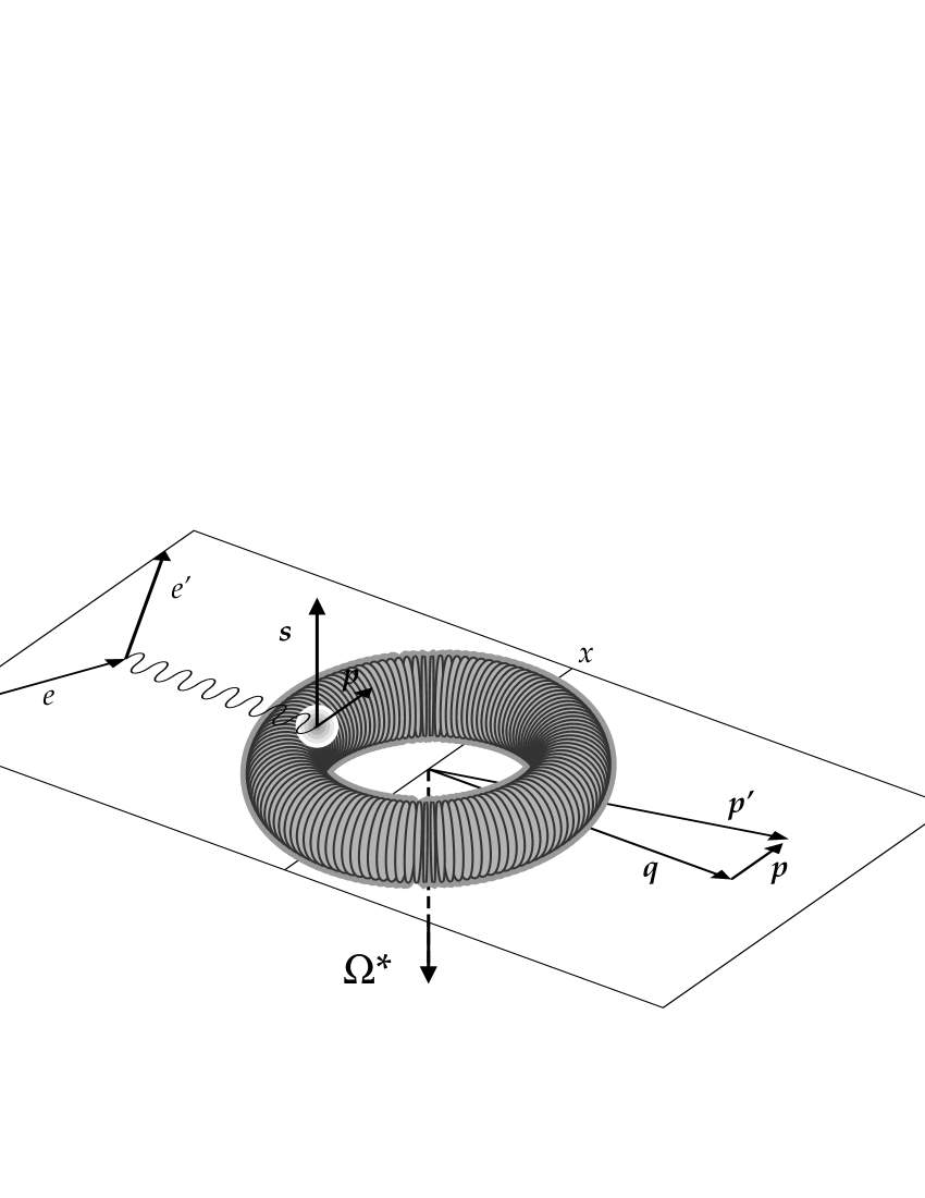
Figure 11: Nucleon orbit for in-plane emission and nodal polarization $(\theta^{*},\Delta\phi)=(90^{\rm o},90^{\rm o})$. The expected value of the proton’s location for the given missing momentum is represented by the white ball. In this case the nucleon spin is opposite to the polarization vector $\mbox{\boldmath$\Omega$}^{*}$. The $z$-axis lies in the direction of q.

Now in the case of the HD cross section a new element comes into play, namely the spin vector, Eq. (56), which for the kinematics of Fig. 11 is given by ${\bf s}=-\mbox{\boldmath$\Omega$}$, since ${\bf p}$ is perpendicular to $\Omega$.

In PWIA the HD response functions in Eq. (16) are proportional to the scalar product between ${\bf s}({\bf p})$ and a single-nucleon vector, Eqs. (18,19). For in-plane emission, $\phi=0^{\rm o}$, the pieces containing $\sin\phi$ do not contribute and hence the single-nucleon vectors are

$${\bf w}_{V}^{T^{\prime}} = 2J_{c}J_{m}\delta\,{\bf e}_{1}-2J_{m}^{2}{\bf e}_{3}$$ (61)

$${\bf w}_{V}^{TL^{\prime}} = 2\sqrt{2}\rho_{c}J_{m}{\bf e}_{1}-2\sqrt{2}\rho_{so}J_{m}\delta\,{\bf e}_{3}.$$ (62)

An important result that follows from these equations is that both single-nucleon vectors lie in the scattering plane. Hence, the HD cross section is determined only by the projection of the nucleon spin in the scattering plane. Since in Fig. 11 the spin is perpendicular to this plane, we have $\Delta=0$ for the nodal polarization $(90^{\rm o},90^{\rm o})$ and the same happens for the opposite polarization $(270^{\rm o},270^{\rm o})$, where the spin is inverted.

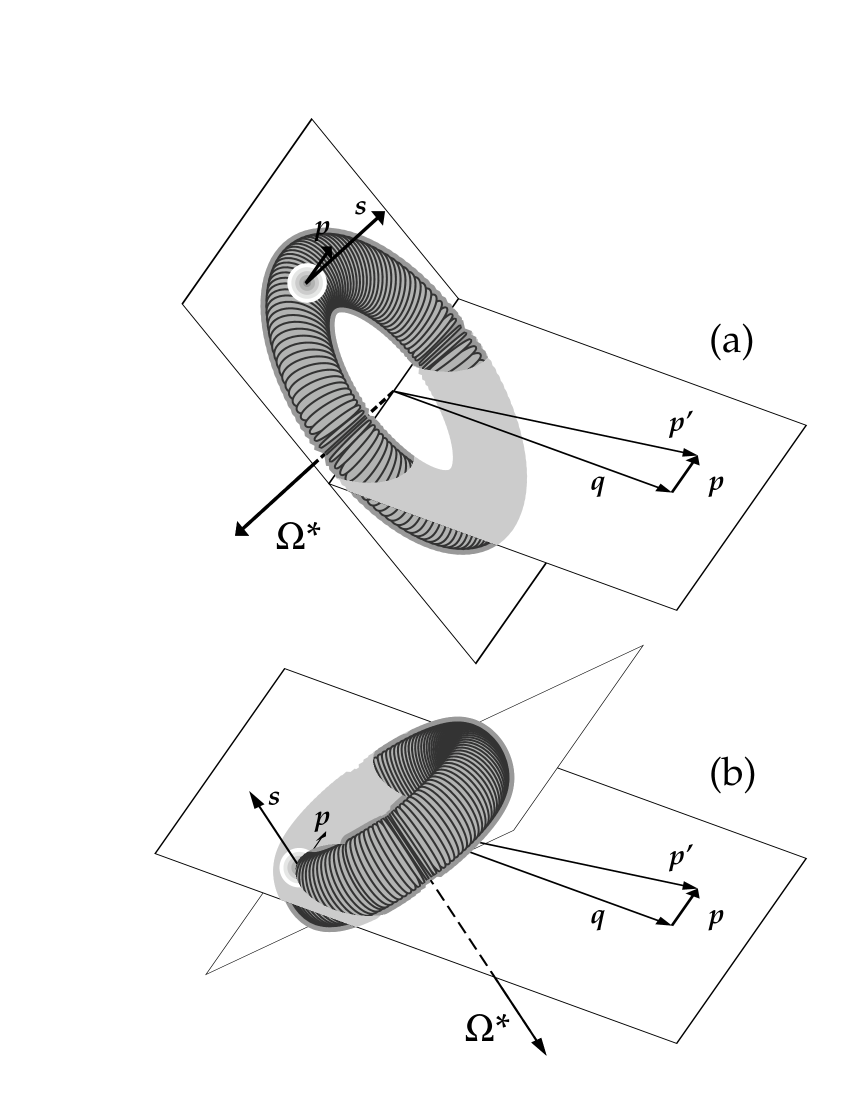
Figure 12: Nucleon orbit for two nuclear polarizations that are symmetrical with respect to the nodal polarization, obtained by $\pm 45^{\rm o}$ rotation of the orbit of Fig. 11 with respect to the $x$-axis. Also shown are the nucleon location and spin for the given missing momentum.

The origin of the nodal symmetry must come from pairs of polarizations with different spins but opposite projections on the scattering plane. An example is show in Fig. 12, corresponding to $\pm 45^{\rm o}$ rotations of the nucleon orbit around the $x$-axis. Fig. 12(a) corresponds to the polarization $(\theta^{*},\Delta\phi)=(135^{\rm o},90^{\rm o})$, while (b) stands for $(45^{\rm o},90^{\rm o})$. These polarizations correspond to a pair of panels in Fig. 1. In Fig. 12 we see that the spin vectors for (a) and (b) point in different directions, although their projections on the scattering plane are equal and opposite. We also see that the proton is located at the same point in the respective orbits, hence with equal values of the scalar momentum distribution. Therefore the corresponding HD cross sections are expected to be equal and opposite in PWIA, as was found for the results shown in Fig. 1. Now the question of why the symmetry persists even in presence of FSI can also be answered using the present example. In fact, from Fig. 12 we see that the proton in (a) and (b) is located in symmetrical positions with respect to the $x$-$z$ plane, above and below the plane, respectively. In the two cases the proton exits the nucleus with the same momentum ${\bf p}^{\prime}$ from positions that are symmetrical with respect to it, traversing equivalent paths across the nucleus and hence experiencing the same interaction (absorption) due to the imaginary part of the central optical potential. Since in both cases the initial impact parameter is also the same, the interaction due to the real part of the central optical potential is also the same.

It remains to be shown that the effect of the spin-orbit part of the potential is also the same in the two cases. This is not obvious a priori because the proton spins in (a) and (b) are different. However, the scalar product ${\bf l}\cdot{\bf s}$ is what enters in the spin-orbit interaction, and remarkably this scalar product is also the same in both cases. In fact, in the semi-classical model the proton exits the nucleus with angular momentum ${\bf l}={\bf r}\times{\bf p}^{\prime}$ and initially with spin ${\bf s}$. Hence the spin-orbit interaction is

$$V_{ls}(r)({\bf r}\times{\bf p}^{\prime})\cdot{\bf s}=-V_{ls}(r)({\bf r}\times{\bf s})\cdot{\bf p}^{\prime}.$$ (63)

In Fig. 12 we see that the value of the vector ${\bf r}\times{\bf s}$ is the same both in cases (a) and (b), since so is the angle between the vectors ${\bf r}$ and ${\bf s}$, and the sense of the vector product is in the $x$-direction.

Therefore we have proven within the semi-classical model that the FSI effects are the same for the two orbit orientations displayed in Fig. 12. These effects are manifested in a modification of the PWIA cross section (both the helicity-dependent and -independent pieces), producing a change of the strength and redistribution of the shape. Since the HD cross section in PWIA is opposite for the two polarizations of Fig. 12 and the secondary effect of FSI is the same in the two cases, the HD cross section that results from including the FSI in DWIA is still equal and opposite in both cases.

Figure 13: Spin direction of the proton computed using Eq. (56) for each of the polarizations of Figs. 1 and 2, for $\phi=0^{\rm o}$, and for missing momentum $p=180$ MeV/c. With an arrow we show the projection of the spin on the $x$-$z$ plane. The inserted numbers indicate the value of the $y$ component in each case.

The existence of the nodal symmetry and its persistence in the presence of FSI can be explained in a similar geometrical way for all of the polarizations shown in Figs. 1 and 2. This can be done by noting that for each pair of nodal polarizations the respective orbits can be obtained by performing a rotation of the nodal orbit of Fig. 11 by angles $\pm\tilde{\theta}$ with respect to an axis contained in the $x$-$z$ plane. For instance, in the case of Fig. 12, the $\pm 45^{\rm o}$ rotations were performed with respect to the $x$-axis. For a fixed value of the missing momentum, the value of $\sin\theta^{*}_{p}$ (remember that $\theta^{*}_{p}$ is the angle between ${\bf p}$ and $\mbox{\boldmath$\Omega$}^{*}$) is the same for the two orbits rotated by angles $\pm\tilde{\theta}$, as is shown in the Appendix. Therefore, the value of the scalar momentum distribution given by Eq. (53) is the same for both orbits, since its angular dependence is $\sin^{2}\theta^{*}_{p}$. As a consequence, the helicity-independent response functions and cross section are also equal for this pair of polarizations. In the case of the HD responses there is an additional dependence on the nucleon spin via the scalar product ${\bf w}^{K}_{V}\cdot{\bf s}({\bf p})$. In Fig. 13 we show the spin vector for each one of the polarizations of Figs. 1 and 2, computed using Eq. (56), for a value of the missing momentum fixed to $p=180$ MeV/c. In the figure we can see that the projection of the spin on the scattering plane is opposite for each pair of polarizations lying symmetrical with respect to the nodal one, for which ${\bf s}$ is perpendicular to the plane. Since the single-nucleon vectors ${\bf w}^{K}_{V}$ are contained in this plane, we find opposite values of ${\bf w}^{K}_{V}\cdot{\bf s}$ for each pair of symmetrical polarizations. This proves that the HD responses are odd with respect to the nodal symmetry in PWIA. An analytical proof of this result is provided in the Appendix.

In arguing that the nodal symmetry persists in presence of the FSI in Fig. 14 we show a plot of the nucleon position within the nucleus and spin vectors for the polarizations of Figs. 1 and 2. The nucleon position has been computed using Eq. (58) for $p=180$ MeV/c. To help in the visualization, in each plot of Fig. 14 we display the exit plane spanned by the vectors ${\bf r}$ and ${\bf p}^{\prime}$, in a coordinate system with the $y$-axis pointing in the ${\bf p}^{\prime}$ direction. In the figure we can see that the initial position of the nucleon is the same for each pair of polarizations lying symmetrical with respect to the nodal point, which implies the same FSI due to the central part of the optical potential for these polarizations. This result is proven analytically in the Appendix.

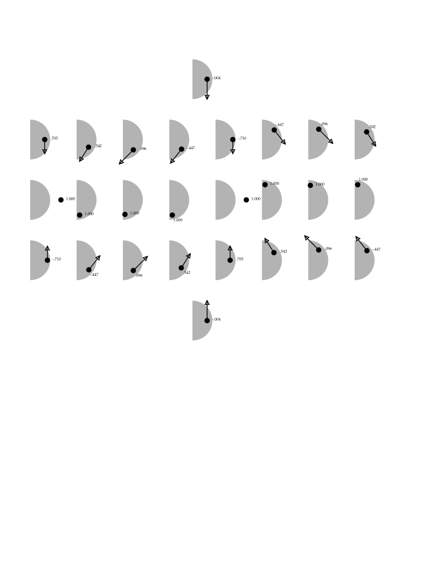
Figure 14: Expected value of position computed using Eq. (58) for each of the polarizations of Figs. 1 and 2, for $\phi=0^{\rm o}$ and for missing momentum $p=180$ MeV/c. The gray semi-circles represent half a slice of the nuclear interior. The coordinate system in the figure is chosen in each case to be the exit plane spanned by the vectors ${\bf r}$ and ${\bf p}^{\prime}$, which is pointing in the $y$-direction in all cases. The arrows represent the spin projection on this plane, while with the inserted numbers we indicate the perpendicular component of the spin.

Moreover, the effect of the spin-orbit FSI can also be inferred from the figure, where we show the projection of the spin on the exit plane. Since the final angular momentum ${\bf r}\times{\bf p}^{\prime}$ is perpendicular to the exit plane, the spin-orbit coupling ${\bf l}\cdot{\bf s}$ is determined only by the perpendicular component of the spin (indicated with the inserted numbers in Fig. 14), and where again we can see that these values are the same for pairs of polarizations that are symmetrical with respect to the nodal point. This implies the same spin-orbit interaction for these polarizations, and is also proven analytically in the Appendix.

These arguments show that the origin of the nodal symmetry in the HD response functions and $\Delta$ in the presence of FSI can be explained in the semi-classical model for $\phi=0^{\rm o}$. Next we discuss the case $\phi=90^{\rm o}$. We have seen in the previous section that in this case the nodal symmetry is broken for the HD cross section $\Delta$ because the $T^{\prime}$ and $TL^{\prime}$ responses present odd and even nodal symmetry respectively. The reason for this different behavior of the $T^{\prime}$ and $TL^{\prime}$ response functions comes from the single-nucleon vectors, Eqs. (18,19), which for $\phi=90^{\rm o}$ can be written as

$${\bf w}_{V}^{T^{\prime}} = 2J_{c}J_{m}\delta\,{\bf e}_{2}-2J_{m}^{2}{\bf e}_{3}$$ (64)

$${\bf w}_{V}^{TL^{\prime}} = 2\sqrt{2}(\rho_{c}J_{m}-J_{c}\rho_{so}\delta^{2}){\bf e}_{1}.$$ (65)

Note the essential difference between the former case, $\phi=0^{\rm o}$, where both single-nucleon vectors were contained in the scattering plane, and the present case, where the $T^{\prime}$ and $TL^{\prime}$ vectors are perpendicular, with the latter pointing to the $x$-direction.

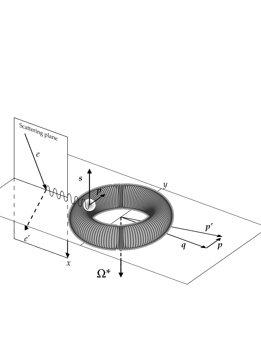
Figure 15: Nucleon orbit for out-of-plane emission, $\phi=90^{\rm o}$, and for the nodal polarization $(\theta^{*},\Delta\phi)=(90^{\rm o},90^{\rm o})$. Note that the only geometrical difference from Fig. 11 is that in this case the scattering plane is perpendicular to the reaction plane.

The differences from the case $\phi=0^{\rm o}$ can be better appreciated by looking at Fig. 15 where it is clear that now the scattering plane ($xz$) is perpendicular to the reaction plane ($yz$). The nucleon orbit shown in Fig. 15 corresponds to the new nodal polarization $(\theta^{*},\Delta\phi)=(90^{\rm o},90^{\rm o})$. Note that in this case $\Delta\phi=90^{\rm o}-\phi^{*}$, so the nodal polarization corresponds to $\phi^{*}=0^{\rm o}$, i.e., $\mbox{\boldmath$\Omega$}^{*}={\bf e}_{1}$, and the nucleon orbit lies in the reaction plane. Comparing Fig. 15 with Fig. 11 we note that the only difference between them lies in the scattering plane spanned by the electrons, which in one case coincides with the reaction plane and is perpendicular in the other. However, the mechanisms underlying the reaction that have to do with the proton orbit and FSI, viz., those that occur in the reaction plane, are identical in both cases.

In fact, we can easily transform the $\phi=90^{\rm o}$ case into the $\phi=0^{\rm o}$ one by just making a change of coordinates

$$x^{\prime}=y,\kern 56.9055pty^{\prime}=-x,\kern 56.9055ptz^{\prime}=z$$ (66)

under which the reaction plane is now the $x^{\prime}z^{\prime}$ plane. Therefore all of the details studied in the case $\phi=0^{\rm o}$ concerning the nucleon orbit, position, spin and FSI effects are also valid in the present case. In particular, Fig. 13 represents the components of the spin in the new reaction plane, corresponding to the polarizations of Figs. 3 and 4, while the proton positions and components of the spin in the exit plane shown in Fig. 14 are also valid in this case.

The only difference with the former case is hence in the single-nucleon vectors of Eqs. (64,65), which in the present case written in the new coordinates are given by

$${\bf w}_{V}^{T^{\prime}} = 2J_{c}J_{m}\delta\,{\bf e}^{\prime}_{1}-2J_{m}^{2}{\bf e}^{\prime}_{3}$$ (67)

$${\bf w}_{V}^{TL^{\prime}} = -2\sqrt{2}(\rho_{c}J_{m}-J_{c}\rho_{so}\delta^{2}){\bf e}^{\prime}_{2}.$$ (68)

Hence the $T^{\prime}$ vector is in the $x^{\prime}z^{\prime}$ plane, while in the former case it was contained in the $xz$ plane. Therefore the behavior of the $T^{\prime}$ response function is exactly the same as in the $\phi=0^{\rm o}$ case. In particular, it is odd under the nodal symmetry. This was expected, because it is known that this response is only a function of $\Delta\phi$, and this is a consequence of the fact that the single-nucleon vector ${\bf w}^{T^{\prime}}_{V}$ is always contained in the reaction plane.

The difference hence lies in the $TL^{\prime}$ response, since now the single-nucleon vector ${\bf w}_{V}^{TL^{\prime}}$ is perpendicular to the reaction plane, while in the former case it was contained in that plane. For this reason, the behavior of the $TL^{\prime}$ response in PWIA now depends on the spin component perpendicular to the reaction plane, which is shown by the inserted numbers in Fig. 13. Therein we can see that this spin component is the same for pairs of polarizations that are symmetrical with respect to the nodal point. Therefore in this case there is no change of sign of the $TL^{\prime}$ response under the nodal symmetry, from which it follows that this response is even under that symmetry, as was seen in the results of Figs. 9 and 10.

These arguments help to clarify the fact that there are actually two reasons why the fifth response function arising for $\phi=90^{\rm o}$ is different from zero for unpolarized nuclei when integrating over all orientations of the nucleon orbit: the first, well-known reason is that the nucleon’s path through the nucleus is different from one polarization to the opposite and hence undergoes different FSI. The second reason is that this response involves the component of the nucleon spin perpendicular to the reaction plane — i.e., in the $x$ direction — and this component is the same for pairs of polarizations that are symmetrical with respect to the nodal one — corresponding to the nucleon orbit being contained in the reaction plane.

4 Conclusions

In this work we have studied the helicity-dependent part of the cross section for $(e,e^{\prime}p)$ reactions with polarized beam and target. Using the shell model to describe the nuclear structure involved, we have presented results of a DWIA calculation for proton knock-out from the $d_{3/2}$ shell of polarized ³⁹K under quasielastic kinematics for the full range of nuclear polarization directions. Such an analysis, performed as a function of the polarization angles, has allowed us to discover a new symmetry in the HD cross section that arises for in-plane emission. This entails a change of sign for pairs of polarization vectors that are opposite with respect to the nodal polarization (i.e., perpendicular to the reaction plane). It is as a consequence of this nodal symmetry that the fifth response function is zero for unpolarized nuclei in these conditions even in presence of FSI.

Our results also show that the nodal symmetry is broken for out-of-plane emission. However, we have found that the symmetry is still present in the three separate response functions $W^{T^{\prime}}$, $\widetilde{W}^{TL^{\prime}}$ and $W^{TL^{\prime}}$, but is not of a single type: while the first two responses are odd under the nodal symmetry, the latter is even, and a linear combination of the three responses therefore breaks the symmetry in the cross section.

The next goal of the paper has been to explain the origin of the nodal symmetry within a semi-classical model of the reaction based on the PWIA and on the concept of a nucleon’s orbit with attendant expectation values of position and spin, and in which the exiting nucleon’s path through the nucleus determines the strength of the FSI. We have shown that for pairs of nodal-symmetrical polarizations the nucleon positions and initial impact parameters are equivalent and with equal values of the spin-orbit coupling ${\bf l}\cdot{\bf s}$, explaining why the FSI effects are the same for these polarizations. The FSI modify the PWIA response functions, which are determined by the scalar product ${\bf w}^{K}_{V}\cdot{\bf s}$, where ${\bf s}$ is the nucleon spin and ${\bf w}^{K}_{V}$ is the single-nucleon vector. We have shown that the component of the spin in the reaction plane changes sign under the nodal symmetry, while the component perpendicular to this plane is invariant under it. As a consequence, since the $T^{\prime}$ single-nucleon vector is always contained in the reaction plane, the $T^{\prime}$ response is always odd under the nodal symmetry. On the other hand, for in-plane emission, the $TL^{\prime}$ single-nucleon vector is also contained in the reaction plane, so the $TL^{\prime}$ response is also odd in these conditions. However, in the case $\phi=90^{\rm o}$ the $TL^{\prime}$ single-nucleon vector is perpendicular to the reaction plane, and so the corresponding $TL^{\prime}$ response is even under the nodal symmetry.

As a consequence of the above, the fifth response function for scattering of polarized electrons from unpolarized nuclei (obtained as an average over orbit orientations) is not zero, and furthermore, in addition to requiring FSI to occur, it probes the spin component of the nucleon perpendicular to the reaction plane.

We would like to emphasize that, although the existence of the nodal symmetry has been found here numerically within the context of a particular DWIA model and proven analytically only in the semi-classical model, there is clear evidence that this is a general, model-independent property of the cross section. This is supported by the fact that the fifth response function is known theoretically to be zero for in-plane emission, so the cancellation between pairs of polarizations must be exact. To provide an analytical, model-independent proof of this theorem from general principles appears not to be a trivial task. However, the results of the present study are clear motivation to find a general symmetry-based proof starting from the formalism of [1, 3].

The success of the present model in explaining the properties of the HD cross section where the proton spin plays a relevant role opens the possibility of using this type of reaction to study not only the 3-dimensional momentum distribution — accessible using polarized nuclei and unpolarized electrons — but also the nucleon spin distribution in nuclei — using in addition polarized electrons. The knowledge gained in the understanding of $(e,e^{\prime}p)$ spin observables through this kind of study, where many of the properties of the cross section, including FSI can be characterized in a clear geometrical picture of the reaction, can be of great help in the design of future experiments with polarized nuclei and electrons. As seen through the examples presented in this paper, this could play an important role in advancing our knowledge of nuclear dynamics.

Appendix: Proof of the nodal symmetry in the semi-classical model

We consider the in-plane emission case, $\phi=0^{\rm o}$, with a fixed value of the missing momentum ${\bf p}$. Remember that in this case the single-nucleon vectors ${\bf w}^{T^{\prime}}_{V}$ and ${\bf w}^{TL^{\prime}}_{V}$ are also contained in the scattering plane, as they are given by Eqs. (61,62). We take as reference the nodal polarization corresponding to $\theta^{*}=90^{\rm o}$, $\phi^{*}=-90^{\rm o}$, i.e., $\mbox{\boldmath$\Omega$}^{*}=-{\bf e}_{2}$. In this case the nucleon orbit lies in the scattering plane as displayed in Fig. 11. If we rotate the nodal orbit by an angle $\tilde{\theta}$ around an axis contained in the scattering plane then

i) the helicity-independent cross section $\Sigma$ is the same for rotation angles $\pm\tilde{\theta}$, and

ii) the HD cross section $\Delta$ has opposite signs for $\pm\tilde{\theta}$.

To prove this, let us consider two polarization vectors, $\mbox{\boldmath$\Omega$}_{1}$ and $\mbox{\boldmath$\Omega$}_{2}$, that are symmetrical with respect to the nodal polarization

$$\mbox{\boldmath$\Omega$}_{1} = \sin\tilde{\theta}\,\mbox{\boldmath$\Omega$}_{s}-\cos\tilde{\theta}\,{\bf e}_{2}$$ (69)

$$\mbox{\boldmath$\Omega$}_{2} = -\sin\tilde{\theta}\,\mbox{\boldmath$\Omega$}_{s}-\cos\tilde{\theta}\,{\bf e}_{2},$$ (70)

where $\mbox{\boldmath$\Omega$}_{s}$ is a unitary vector contained in the scattering plane, i.e.,

$$\mbox{\boldmath$\Omega$}_{s}=\cos\tilde{\phi}\,{\bf e}_{1}+\sin\tilde{\phi}\,{\bf e}_{3}.$$ (71)

Then the following results emerge:

1. The projections of $\mbox{\boldmath$\Omega$}_{1}$ and $\mbox{\boldmath$\Omega$}_{2}$ over the missing momentum ${\bf p}$ have opposite sign, since ${\bf p}$ lies in the scattering plane, i.e.,

   $$\mbox{\boldmath$\Omega$}_{1}\cdot{\bf p}=-\mbox{\boldmath$\Omega$}_{2}\cdot{\bf p}=\sin\tilde{\theta}\,\mbox{\boldmath$\Omega$}_{s}\cdot{\bf p}.$$ (72)

   Hence the angles $\theta^{*}_{p1}$ and $\theta^{*}_{p2}$ between ${\bf p}$ and the polarization vectors $\mbox{\boldmath$\Omega$}_{1}$ and $\mbox{\boldmath$\Omega$}_{2}$ satisfy

   $$\cos\theta^{*}_{p1} = -\cos\theta^{*}_{p2}$$ (73)

   $$\sin\theta^{*}_{p1} = \sin\theta^{*}_{p2}.$$ (74)

   As a consequence, since the scalar momentum distribution for the $d_{3/2}$ shell is $M_{s}=\frac{3}{8\pi}\sin^{2}\theta^{*}_{p}|\tilde{R}(p)|^{2}$, and the value of $\sin\theta^{*}_{pi}$ is the same for these two polarizations, the helicity-independent response functions in Eq. (15) are the same for these two polarizations in PWIA, and hence so are the cross sections $\Sigma$ in PWIA.

2. Let ${\bf s}_{1}$ and ${\bf s}_{2}$ be the spin vectors for these two orbits, given by Eq. (56). Then this pair of spins has opposite components on the scattering plane and equal components on the $y$-axis. In fact we have, from Eq. (56),

   $${\bf s}_{1} = \frac{2\mbox{\boldmath$\Omega$}_{1}\cdot{\bf p}}{p^{2}}{\bf p}-\mbox{\boldmath$\Omega$}_{1}=\frac{2\sin\tilde{\theta}\,\mbox{\boldmath$\Omega$}_{s}\cdot{\bf p}}{p^{2}}{\bf p}-\sin\tilde{\theta}\,\mbox{\boldmath$\Omega$}_{s}+\cos\tilde{\theta}\,{\bf e}_{2}$$ (75)

   $${\bf s}_{2} = \frac{2\mbox{\boldmath$\Omega$}_{2}\cdot{\bf p}}{p^{2}}{\bf p}-\mbox{\boldmath$\Omega$}_{2}=-\frac{2\sin\tilde{\theta}\,\mbox{\boldmath$\Omega$}_{s}\cdot{\bf p}}{p^{2}}{\bf p}+\sin\tilde{\theta}\,\mbox{\boldmath$\Omega$}_{s}+\cos\tilde{\theta}\,{\bf e}_{2};$$ (76)

   hence the spin components on the scattering plane, $({\bf s}_{i})_{s}$, are opposite and satisfy

   $$({\bf s}_{1})_{s}=-({\bf s}_{2})_{s}=\sin\tilde{\theta}\left(\frac{2\mbox{\boldmath$\Omega$}_{s}\cdot{\bf p}}{p^{2}}{\bf p}-\mbox{\boldmath$\Omega$}_{s}\right),$$ (77)

   while the $y$-components are equal and given by

   $$({\bf s}_{1})_{y}=({\bf s}_{2})_{y}=\cos\tilde{\theta}\,{\bf e}_{2}.$$ (78)

   Since the single-nucleon vectors in Eqs. (61,62) are in the scattering plane, their scalar products with the spin vectors ${\bf s}_{i}$ are opposite, as are also the HD response functions $T^{\prime}$ and $TL^{\prime}$ in PWIA; i.e., they are odd with respect to the nodal symmetry. The same result holds for the HD cross section $\Delta$.

3. Let ${\bf r}_{1}$ and ${\bf r}_{2}$ the expected values of position of the nucleon for the two polarizations $\mbox{\boldmath$\Omega$}_{1}$, $\mbox{\boldmath$\Omega$}_{2}$. Then ${\bf r}_{1}$ and ${\bf r}_{2}$ have opposite projections on the scattering plane and equal projections on the $y$-axis. In fact, from Eq. (58) we have

   $${\bf r}_{i}=-\frac{1+\sin^{2}\theta^{*}_{pi}}{p^{2}\sin^{2}\theta^{*}_{pi}}\mbox{\boldmath$\Omega$}_{i}\times{\bf p}.$$ (79)

   By result 1, $\sin\theta^{*}_{p1}=\sin\theta^{*}_{p2}$ and therefore the factor in front of $\mbox{\boldmath$\Omega$}_{i}\times{\bf p}$ is the same for ${\bf r}_{1}$ and ${\bf r}_{2}$. Furthermore, we have for the vector products

   $$\mbox{\boldmath$\Omega$}_{1}\times{\bf p} = \sin\tilde{\theta}\,\mbox{\boldmath$\Omega$}_{s}\times{\bf p}-\cos\tilde{\theta}\,{\bf e}_{2}\times{\bf p}$$ (80)

   $$\mbox{\boldmath$\Omega$}_{2}\times{\bf p} = -\sin\tilde{\theta}\,\mbox{\boldmath$\Omega$}_{s}\times{\bf p}-\cos\tilde{\theta}\,{\bf e}_{2}\times{\bf p}.$$ (81)

   We compute separately the two vector products above. From the first one we obtain the projection on the $y$-axis

   $$\mbox{\boldmath$\Omega$}_{s}\times{\bf p} = p(\cos\tilde{\phi}\,{\bf e}_{1}+\sin\tilde{\phi}\,{\bf e}_{3})\times(\sin\theta\,{\bf e}_{1}+\cos\theta\,{\bf e}_{3})$$ (82)

   $$= p(\sin\tilde{\phi}\sin\theta-\cos\tilde{\phi}\cos\theta){\bf e}_{2},$$

   while for the second one we obtain the projection on the scattering plane

   $${\bf e}_{2}\times{\bf p}=p{\bf e}_{2}\times(\sin\theta\,{\bf e}_{1}+\cos\theta\,{\bf e}_{3})=p(\cos\theta\,{\bf e}_{1}-\sin\theta\,{\bf e}_{3}).$$ (83)

   Therefore we obtain for the position vectors

   $${\bf r}_{1} = \frac{1+\sin^{2}\theta^{*}_{p1}}{p\sin^{2}\theta^{*}_{p1}}\left[-\sin\tilde{\theta}(\sin\tilde{\phi}\sin\theta-\cos\tilde{\phi}\cos\theta){\bf e}_{2}-\cos\tilde{\theta}(\cos\theta\,{\bf e}_{1}-\sin\theta\,{\bf e}_{3})\right]$$

   $${\bf r}_{2} = \frac{1+\sin^{2}\theta^{*}_{p1}}{p\sin^{2}\theta^{*}_{p1}}\left[\sin\tilde{\theta}(\sin\tilde{\phi}\sin\theta-\cos\tilde{\phi}\cos\theta){\bf e}_{2}+\cos\tilde{\theta}(\cos\theta\,{\bf e}_{1}-\sin\theta\,{\bf e}_{3})\right].$$

   From these equations we obtain the desired result.

4. The projections of ${\bf r}_{1}$ and ${\bf r}_{2}$ over the exit vector ${\bf p}^{\prime}$ are the same, and the exit impact parameters $b_{1}$ and $b_{2}$ are equal. In fact, the first result follows from point 3 above, since ${\bf p}^{\prime}$ is in the scattering plane and both vectors ${\bf r}_{1}$ an ${\bf r}_{2}$ have the same component in this plane. On the other hand, the impact parameter is defined with respect to the exit direction ${\bf p}^{\prime}$ as the modulus of the perpendicular component of ${\bf r}$ with respect to ${\bf p}^{\prime}$, i.e.,

   $${\bf b}={\bf r}-\frac{{\bf r}\cdot{\bf p}^{\prime}}{p^{\prime}{}^{2}}{\bf p}^{\prime}.$$ (86)

   Since ${\bf r}_{1}\cdot{\bf p}^{\prime}={\bf r}_{2}\cdot{\bf p}^{\prime}$ and, from point 3, $|{\bf r}_{1}|=|{\bf r}_{2}|$, the components of ${\bf r}_{1}$ perpendicular to ${\bf p}^{\prime}$ are equal, i.e., $b_{1}=b_{2}$.

   As a direct consequence of this result, if we choose the exit direction ${\bf p}^{\prime}$ as the $z$-axis, then the two nucleons at positions ${\bf r}_{1}$ and ${\bf r}_{2}$ are initially at the same height and with the same impact parameter. Therefore their interaction with the central part of the optical potential along its exit trajectory is the same for both nucleons. This proves the persistence of the nodal symmetry in the presence of the central part of the optical potential.

5. The value of the spin-orbit coupling ${\bf s}\cdot{\bf l}$ for the ejected particle is the same for both polarizations. In fact, the angular momentum of the final proton is

   $${\bf l}={\bf r}\times{\bf p}^{\prime}=-\frac{1+\sin^{2}\theta^{*}_{p}}{p^{2}\sin^{2}\theta^{*}_{p}}(\mbox{\boldmath$\Omega$}^{*}\times{\bf p})\times{\bf p}^{\prime}.$$ (87)

   The double vector product appearing above is given by

   $$(\mbox{\boldmath$\Omega$}^{*}\times{\bf p})\times{\bf p}^{\prime}=(\mbox{\boldmath$\Omega$}^{*}\cdot{\bf p}^{\prime}){\bf p}-({\bf p}\cdot{\bf p}^{\prime})\mbox{\boldmath$\Omega$}^{*}.$$ (88)

   The factor in Eq. (87) depending on $\sin\theta^{*}_{p}$ is the same for both polarizations. Therefore the spin-orbit coupling is determined by the following scalar product

   $${\bf s}\cdot[(\mbox{\boldmath$\Omega$}^{*}\times{\bf p})\times{\bf p}^{\prime}]=(\mbox{\boldmath$\Omega$}^{*}\cdot{\bf p}^{\prime}){\bf p}\cdot{\bf s}-({\bf p}\cdot{\bf p}^{\prime})\mbox{\boldmath$\Omega$}^{*}\cdot{\bf s}.$$ (89)

   Now using Eq. (56) we have for the spin scalar products:

   $${\bf p}\cdot{\bf s} = \frac{2\mbox{\boldmath$\Omega$}^{*}\cdot{\bf p}}{p^{2}}{\bf p}^{2}-\mbox{\boldmath$\Omega$}^{*}\cdot{\bf p}=\mbox{\boldmath$\Omega$}\cdot{\bf p}$$ (90)

   $$\mbox{\boldmath$\Omega$}^{*}\cdot{\bf s} = \frac{2\mbox{\boldmath$\Omega$}^{*}\cdot{\bf p}}{p^{2}}{\bf p}\cdot\mbox{\boldmath$\Omega$}^{*}-1=\left(\frac{2\mbox{\boldmath$\Omega$}^{*}\cdot{\bf p}}{p}\right)^{2}-1.$$ (91)

   Therefore

   $${\bf s}\cdot[(\mbox{\boldmath$\Omega$}^{*}\times{\bf p})\times{\bf p}^{\prime}]=(\mbox{\boldmath$\Omega$}^{*}\cdot{\bf p}^{\prime})(\mbox{\boldmath$\Omega$}^{*}\cdot{\bf p})-({\bf p}\cdot{\bf p}^{\prime})\left[\left(\frac{2\mbox{\boldmath$\Omega$}^{*}\cdot{\bf p}}{p}\right)^{2}-1\right].$$ (92)

   Since the projections of $\mbox{\boldmath$\Omega$}_{1}$ and $\mbox{\boldmath$\Omega$}_{2}$ on the scattering plane are opposite, and both ${\bf p}$ and ${\bf p}^{\prime}$ are contained in that plane, we have

   $$(\mbox{\boldmath$\Omega$}_{1}\cdot{\bf p}^{\prime})(\mbox{\boldmath$\Omega$}_{1}\cdot{\bf p}) = (\mbox{\boldmath$\Omega$}_{2}\cdot{\bf p}^{\prime})(\mbox{\boldmath$\Omega$}_{2}\cdot{\bf p})$$ (93)

   $$(\mbox{\boldmath$\Omega$}_{1}\cdot{\bf p})^{2} = (\mbox{\boldmath$\Omega$}_{2}\cdot{\bf p})^{2}$$ (94)

   from which it follows that

   $${\bf s}_{1}\cdot{\bf l}_{1}={\bf s}_{2}\cdot{\bf l}_{2}.$$ (95)

   Hence the spin-orbit interaction is the same for both polarizations.

References

- [1] J.E. Amaro and T.W. Donnelly, Ann. Phys. (N.Y.) 263 (1998) 56.
- [2] J.E. Amaro and T.W. Donnelly, Nucl. Phys. A646 (1999) 187.
- [3] A.S. Raskin and T.W. Donnelly, Ann. Phys. (N.Y.) 191 (1989) 78.
- [4] J.E. Amaro, J.A. Caballero, T.W. Donnelly and E. Moya de Guerra, Nucl. Phys. A611 (1996) 163.
- [5] A. Bianconi and M. Radici, Phys. Rev. C53 (1996) 563.
- [6] J.A. Caballero, T.W. Donnelly and G.I. Poulis, Nucl. Phys. A555 (1993) 709.
- [7] J.A. Caballero, T.W. Donnelly, G.I. Poulis, E. Garrido and E. Moya de Guerra, Nucl. Phys. A577 (1994) 528.
- [8] J.A. Caballero, E. Garrido, E. Moya de Guerra, P. Sarriguren, J.M. Udias, Ann. Phys. 239 (1995) 351.
- [9] S. Boffi, C. Giusti and F.D. Pacati, Nucl. Phys A476 (1988) 617.
- [10] E. Garrido, J.A. Caballero, E. Moya de Guerra, P.Sarriguren and J.M. Udias, Nucl. Phys. A584 (1995) 256.
- [11] H. Arenhövel, W. Leidemann and E.L. Tomusiak, Phys. Rev. C46 (1992) 455.
- [12] A. Bianconi and M. Radici, Phys. Rev. C56 (1997) 1002.
- [13] S. Jeschonnek and T. W. Donnelly, Phys.Rev. C59 (1999) 2676.
- [14] J.E. Amaro, J.A. Caballero, T.W. Donnelly, A.M. Lallena, E. Moya de Guerra and J.M. Udias, Nucl. Phys. A602 (1996) 263.
- [15] J.E. Amaro, M.B. Barbaro, J.A. Caballero, T.W. Donnelly and A. Molinari Nucl. Phys. A643 (1998) 349.
- [16] S. Galster et al., Nucl. Phys. B32 (1971) 221.
- [17] J. M. Udias, J. A. Caballero, E. Moya de Guerra, J. E. Amaro and T. W. Donnelly, Phys. Rev. Lett. 83 (1999) 5451.
- [18] J.E. Amaro, G. Co’ and A.M. Lallena, Nucl. Phys. A578 (1994) 365.
- [19] P. Schwandt et al., Phys. Rev. C26 (1982) 55.