QUADRUPOLE OSCILLATIONS AS PARADIGM OF THE CHAOTIC MOTION IN NUCLEI. Part 2

The present communication is a continuation of the review, the first part of which was presented in nucl-th 0109033. The second part dealswith the manifistation of Chaotic dynamics at quantum level. The variations of statistical properties of energy spectrum in the process of $R-C-R$ transition have been studied in detail. We proved that the type of the classical motion is correlated with the structure of the eigenfunctions of highly excited states in the $R-C-R$ transition. Shell structure destruction induced by the increase of nonintegrable perturbation was analyzed.

PACS numbers: 05.45.+b, 24.60.La, 21.10.-k, 03.65. Sq.

1 Quantum manifestations of the classical
stochasticity

1.1 The quantum chaos problem

Essential progress in the understanding of the nonlinear dynamics of classical systems stimulated numerous attempts to include the conception of the stochasticity in quantum mechanics [3, 4, 10, 11, 12, 13, 14]. The essence of the problem consists in the fact that the energy spectrum of any quantum system, performing the finite motion, is discrete and therefore its evolution is quasiperiodic. At the same time, the correspondence principle requires the possibility of limit transition to classical mechanics, containing not only regular solutions but also chaotic ones. The total solving of this problem is too complicated one, therefore its restricted variant is of considerable interest. We are interested in the search of peculiarities of behaviour of quantum systems the classical analogs of which reveal chaotic behaviour. Such peculiarities are usually called the quantum manifestations of the classical stochasticity (QMCS).

The following objects can be used as the objects of search of the QMCS for an autonomous systems

1) the energy spectra

2) the stationary wave functions

3) the wave packets.

A priori the manifestations of the QMCS can be expected both in the form of some peculiarities of concrete stationary state and in the whole group of close states in energy. Of course, it is not excepted the possibility that such alternative does not exist at all, i.e. the traces of the classical chaos can be detected both in the properties of separate states and so in their sets.

In this part of the review we will represent the results relating to the QMCS in the dynamics of quadrupole oscillations.

1.2 Numerical procedure

The quantum scaled Hamiltonian describing the quadrupole surface oscillations has the following form

$$H=\frac{{\bar{\hbar}_{i}^{2}}}{2}\left({\Delta_{x}+\Delta_{y}}\right)+U_{i}\left({x,y,W}\right)$$ (1)

where the scaled Planck’s constant is $\bar{\hbar}={\raise 3.01385pt\hbox{$\hbar$}\!\mathord{\left/{\vphantom{\hbar{\hbar_{0i}}}}\right.\kern-1.2pt}\!\lower 3.01385pt\hbox{${\hbar_{0i}}$}}$ , $\hbar_{0i}^{2}=m\varepsilon_{0i}l_{0i}^{2}$ , and scaling parameters $\hbar_{0i},l_{0i}$ and deformation potential $U_{i}(x,y,W)$ are determined by the expressions (21.1) and (23.1). We are going to study the peculiarities of structure of energy spectra and wave functions in each of the following intervals

the first regular region $R_{1}:\quad 0<E<E_{cr1}$

the chaotic region $C:\quad E_{cr1}<E<E_{cr2}$

the second regular region $R_{2}:\quad E>E_{cr2}$.

The critical energies $E_{cr1}$ and $E_{cr2}$ were determined above. The main numerical calculations were performed for one-well potentials ($0<W<16$ ). In this case the critical energies are determined by the relations (60.1), (61.1).

At fixed topology of potential surface $\left({W=const}\right)$ , the scaled Planck’s constant $\bar{\hbar}_{i}$ is the unique free parameter in the quantum Hamiltonian (1). In the study of the concrete region of energies, corresponding to the certain type of classical motion $\left({R_{1},C,R_{2}}\right)$ , the choice of $\bar{\hbar}_{i}$ is dictated by the possibility of attainment the required degree of validity of semiclassical approximation (large quantum numbers) conserving the precision of calculations of spectrum and wave functions (the limitation of the possibility of diagonalization of large dimension matrices). For the original nonreduced Hamiltonian (16.1) the variation of $\bar{\hbar}_{i}$ is equivalent to the variation of the critical energies $E_{cr1}$ and $E_{cr2}$ (i.e. parameters $a,b,c$ ) or to the adequate choice of Planck’s constant $\hbar$ .

The procedure of diagonalization was used for the determination of energy spectrum and eigenfunctions of the Hamiltonian (1). As the basis we chose the simple combinations of the eigenfunctions of the two-dimensional harmonic oscillator with equal frequencies [15]

$$\begin{gathered}\left|{NLj}\right\rangle=\frac{{P_{L,j}}}{{\sqrt{2}}}\left({\left|{NL}\right\rangle+j\left|{N,-L}\right\rangle}\right),j=\pm 1\;\hfill\\ N=0,1,2...;\quad L=N,N-2...1\;\;or\;\;0\hfill\\ \end{gathered}$$ (2)

normalized according to the condition

$$\left\langle{{NLj}}\mathrel{\left|{\vphantom{{NLj}{N^{\prime}L^{\prime}j^{\prime}}}}\right.\kern-1.2pt}{{N^{\prime}L^{\prime}j^{\prime}}}\right\rangle=\frac{1}{{\sqrt{2}}}2^{\delta_{L,0}}\delta_{jj^{\prime}}\delta_{NN^{\prime}}\delta_{LL^{\prime}}$$ (3)

and $P_{L,j}=j^{Mod\left({L,3}\right)}$ .

The symmetry of the considered Hamiltonian $(C_{3v})$ leads to the block structure of matrix $\left\langle{N^{\prime}L^{\prime}j^{\prime}}\right|H\left|{NLj}\right\rangle$ , which consists of four independent submatrices. It allows to carry out diagonalization of each submatrix separately, obtaining in this case four independent sets of states, which according to the classification used in the theory of groups are the following states

$A_{1}$ - type [mode$(L,3)=0,j=1$ , including $L=0$ ]

$A_{2}$ - type [mode$(L,3)=0,j=-1,L\neq 0$ ]

and twice degenerated states

$E$ - type [ mode $(L,3)\neq 0,j=\pm 1$ ]

The possibility of separate diagonalization of submatrices of definite type allows essentially to increase available dimension of basis in numerical calculations (later for brief, we shall call the dimension of basis as the dimension n of separate submatrix). Table 3.2.1 shows the maximum oscillator numbers$N_{0}$ of the basis and the dimension $m$ of total matrix $\left\langle{N^{\prime}L^{\prime}j^{\prime}}\right|H\left|{NLj}\right\rangle$ for the above enumerated types of submatrices with the dimension $n=408$

Table 3.2.1

	$A_{1}$	$A_{2}$	$E_{1,2}$
$N_{0}$	$67$	$70$	$48$
$m$	$2346$	$2556$	$1225$

Expansion of wave eigenfunctions in basis (2) in polar coordinates $r,\varphi$

$$\left\langle{{r,\varphi}}\mathrel{\left|{\vphantom{{r,\varphi}{E_{k}}}}\right.\kern-1.2pt}{{E_{k}}}\right\rangle=\sum\limits_{NL}{C_{NLj}^{\left(k\right)}\left\langle{{r,\varphi}}\mathrel{\left|{\vphantom{{r,\varphi}{NLj}}}\right.\kern-1.2pt}{{NLj}}\right\rangle}$$ (4)

where

$$\left\langle{{r,\varphi}}\mathrel{\left|{\vphantom{{r,\varphi}{NL}}}\right.\kern-1.2pt}{{NL}}\right\rangle=$$ (5)

$$i^{N}\frac{{e^{-iL\varphi}}}{{\sqrt{2\pi}}}\frac{1}{{L!}}\left[{\frac{{2\left({\frac{{N+L}}{2}}\right)!}}{{\left({\frac{{N-L}}{2}}\right)!}}}\right]^{{\raise 2.1097pt\hbox{$1$}\!\mathord{\left/{\vphantom{12}}\right.\kern-1.2pt}\!\lower 2.1097pt\hbox{$2$}}}\left({\sqrt{\omega_{0}}r}\right)^{L}e^{-\omega_{0}{\hbox{${r^{2}}$}\!\mathord{\left/{\vphantom{{r^{2}}2}}\right.\kern-1.2pt}\!\lower 2.1097pt\hbox{$2$}}}M\left\{{-\frac{{N-L}}{2},L+1,\omega_{0}r^{2}}\right\}$$

Here $M\{\quad\}$ is degenerated hypergeometric function and $\omega_{0}$ - frequency of the oscillator basis. The finite dimension of the basis used in calculations leads to the dependence of the position of level from the oscillator frequency $\omega_{0}$ . Such dependence for the dimensions of basis $n=198$ and $n=408$ ($W=13$ ) is represented in Fig.18.

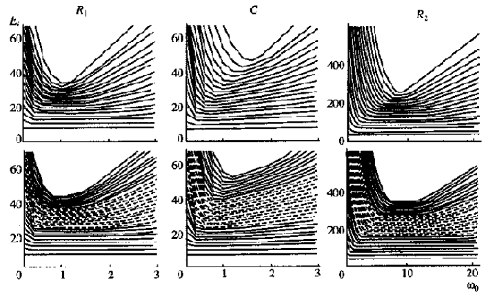
Figure 18: Energy spectra of Hamiltonian (1) as function of the frequency $\omega_{0}$ of the oscillator basis $\left({W=13}\right)$ . The upper and lower parts of this figure show this dependence for the basis dimensions $n=198$ and $n=408$ , respectively.

The important moment of numerical calculations is the choice of the optimal frequency $\omega_{0}n^{opt}$, determined from the condition that the energies of levels, situated in the interval of our interest, have minimum value. Such optimization is essentially important for the regions $C$ and $R_{2}$ , where the position of the levels more depends on the frequency of basis. The optimal frequency depends both on dimension of the basis and on the length of investigated energy interval. As is shown in Fig.18 it is possible to choose the unique frequency $\omega_{0}^{opt}$ for intervals including decades or more levels just at the dimension of the basis $n=408$ . These levels are selected in Fig.18 by dotted lines. The large value of $\omega_{0}^{opt}$ for the region $R_{2}(\omega_{0}^{opt}\sim 8)$ is caused by the fact that at energies $E>E_{cr2}$ the deformation potential essentially differs from harmonic oscillator potential.

The dimension of the basis used in our calculations was determined for the reason of acceptability of the calculation time and the calculation precision of the position of levels in considered region. The results of investigation of saturation in basis are represented in Fig.19, i.e. dependence of the results of spectrum calculation from the dimension of basis. As it is shown in Fig.19 for the regions $R_{1}$ and $R_{2}$ acceptable precision of calculations of levels with ordinal numbers $100-200$ is reached at the dimension of the basis $n\sim 400$ , while for the chaotic region $C$ dimension of the basis required for the attainment of the same precision considerably larger $(n\sim 700)$ . It is a well known result [3, 6]: the value of saturation in basis is sensitive to the type of classical motion.

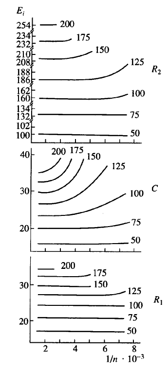
Figure 19: Energy levels as function of the basis dimension $n$ . The numbers on the curves are the level numbers $k$ .

Matrix diagonalization is attractive for treating Hamiltonians that do not differ greatly from Hamiltonians with known eigenfunctions. This numerical procedure becomes less attractive (or even not effective at all) at the transition to the PES of complicated topology, when required Hamiltonian matrix is of high order. In this case the alternative to the diagonalization may become the so-called spectral method [16], which utilizes numerical solutions to the time-dependent Schrodinger equation. The spectral method was developed earlier for determining the eigenvalues and eigenfunctions for the modes of optical waveguides from numerical solutions of the paraxial wave equation [17]. Feit, Fleck and Steiger [16] were able to apply the previously developed methodology to quantum mechanical problems with little change, as the latter equation is identical to the Schrodinger equation.

The spectral method requires computation of the correlation function

$$P_{1}\left(t\right)=\left\langle{{\psi\left({\vec{r},0}\right)}}\mathrel{\left|{\vphantom{{\psi\left({\vec{r},0}\right)}{\psi\left({\vec{r},t}\right)}}}\right.\kern-1.2pt}{{\psi\left({\vec{r},t}\right)}}\right\rangle$$ (6)

where $\psi\left({\vec{r},t}\right)$ represents a numerical solution of the time-dependent Schrodinger equation, and $\psi\left({\vec{r},0}\right)$ is the wave function at $t=0$ . The solution $\psi\left({\vec{r},t}\right)$ can be accurately generated with the help of the split operator FFT (Fast Fourier Transformation) method [18]. The numerical FFT of $P_{1}(t)$ , or $P_{1}(E)$ , displays a set of sharp local maxima for $E=E_{n}$ , where $E_{n}$ are the desired energy eigenvalues. With the aid of lineshape fitting techniques, both the positions and heights of these resonances can be determined with high accuracy. The former yield the eigenvalues and the latter the weights of the stationary states that compose the wave packet once the eigenvalues are known, the corresponding eigenfunctions can be computed by numerically evaluating the integrals

$$\psi\left({\vec{r},E_{n}}\right)=\int\limits_{0}^{T}{\psi\left({\vec{r},t}\right)W\left(t\right)\exp\left({iE_{n}t}\right)dt}$$ (7)

where $T$ is the time encompassed by the calculation, and $W(t)$ is a window function,

$$\begin{gathered}W\left(t\right)=1-\cos{\raise 3.01385pt\hbox{${2\pi t}$}\!\mathord{\left/{\vphantom{{2\pi t}T}}\right.\kern-1.2pt}\!\lower 3.01385pt\hbox{$T$}}\;\;if\quad 0<t<T\hfill\\ \quad\quad=0\quad\quad\quad\quad\quad if\quad\quad\;\;t>T\hfill\\ \end{gathered}$$ (8)

Since the spectral method is fundamentally based on numerical solutions of a time-dependent differential equation, its implementation is always straightforward. No special ad hoc selection of basis function is required, nor is it necessary for the potential to have a special analytic form. The spectral method is in principle applicable to problems involving any number of dimensions.

1.3 Quantization by the normal form

In this section we calculate a semiclassical approximation to an energy spectrum of the Hamiltonian of qudrupole oscillations (1) [19] (here it will be more suitable for us to use the nonscale version of the Hamiltonian (16.1) with $m=1$ ) by quantization the normal form and compare results to exact quantum mechanical calculations. By the exact spectrum we mean the spectrum obtained by the direct numerical calculations, for example, by the diagonalization of the Hamiltonian on the reasonably chosen basis. Quantization the incommensurable case is straightforward. Since the normal form can be expressed entirely in terms of action variables, we merely have to replace those action variables by an appropriate multiple of $\hbar,I_{\nu}\to\hbar\left({n_{\nu}+{\raise 3.01385pt\hbox{$1$}\!\mathord{\left/{\vphantom{12}}\right.\kern-1.2pt}\!\lower 3.01385pt\hbox{$2$}}}\right)$ and the result is a power series in the quantum numbers,

$$E_{n_{1}n_{2}}=\Gamma\left({n_{1}+{\raise 3.01385pt\hbox{$1$}\!\mathord{\left/{\vphantom{12}}\right.\kern-1.2pt}\!\lower 3.01385pt\hbox{$2$}},n_{2}+{\raise 3.01385pt\hbox{$1$}\!\mathord{\left/{\vphantom{12}}\right.\kern-1.2pt}\!\lower 3.01385pt\hbox{$2$}}}\right)$$ (9)

The commensurable case is less straightforward. Commensurability of frequencies leads to the appearance of angle variables in the normal form

$$\Gamma=\Gamma\left({I_{1},I_{2},\varphi_{2}}\right)$$ (10)

As before, the action $I_{1}$ we can replace on $\hbar\left({n_{1}+{\raise 3.01385pt\hbox{$1$}\!\mathord{\left/{\vphantom{12}}\right.\kern-1.2pt}\!\lower 3.01385pt\hbox{$2$}}}\right)$ . In this case the initial two-dimensional problem is reduced to one-dimensional problem, the quantization of which can be performed with the help of WKB method.

The procedure of quantization by normal form we shall begin with canonical transformation

$$\begin{gathered}q_{1}=\frac{i}{2}\left({-Q_{1}+Q_{2}+P_{1}-P_{2}}\right)\hfill\\ q_{2}=\frac{1}{2}\left({Q_{1}+Q_{2}+P_{1}+P_{2}}\right)\hfill\\ p_{1}=\frac{1}{2}\left({Q_{1}-Q_{2}+P_{1}-P_{2}}\right)\hfill\\ p_{2}=\frac{i}{2}\left({Q_{1}-Q_{2}-P_{1}-P_{2}}\right)\hfill\\ \end{gathered}$$ (11)

where variables $(\vec{p},\vec{q})$ provide reduction of the harmonic part of the initial Hamiltonian (16.1) to the form (77.1). In the new variables $\vec{Q}(Q_{1},Q_{2})$ and $\vec{P}(P_{1},P_{2})$ the Hamiltonian of quadrupole oscillations is the following

$$K\left({\vec{Q},\vec{P}}\right)=K^{\left(2\right)}\left({\vec{Q},\vec{P}}\right)+\sum\limits_{j>2}{K^{\left(j\right)}\left({\vec{Q},\vec{P}}\right)}$$ (12)

where

$$K^{\left(2\right)}\left({\vec{Q},\vec{P}}\right)=i\left({Q_{1}P_{1}+Q_{2}P_{2}}\right)$$ (13)

and $K^{(j)}$ are homogeneous polynomials in variables $Q_{i}$ and $P_{i}$ of degree $j$. Each member $K^{(j)}$ of the Hamiltonian (12) is reduced to the normal form according to the procedure describing in the section 2.5(part 1). However this procedure is sufficiently simplified due to the diagonal form of the operator $D$ in the variables $(\vec{P},\vec{Q})$. The classical normal form is the sum of the polynomials of special form in $Q_{i}$ and $P_{i}$ . For obtaining its quantum analog we can use the Weyl’s heuristic rule of correspondence [20, 21]

$$P^{n}Q^{m}=Q^{m}P^{n}\to\frac{1}{{2^{n}}}\sum\limits_{l=0}^{n}{\frac{{n!}}{{l!\left({n-l}\right)!}}}\hat{Q}^{m}\hat{P}^{n-l}$$ (14)

The operators $\hat{P}_{i}$ and $\hat{Q}_{i}$ are determined by formulae (11), in which by $p_{i}$ and $q_{i}$ we should mean operators of impulse and coordinate with usual rules of commutation, from which it follows that

$$\left[{\hat{P}_{k},\hat{Q}_{l}}\right]=\delta_{kl}\left({k,l=1,2}\right)$$ (15)

The operators $\hat{P}_{i}$ , $\hat{Q}_{i}$ allow to introduce the full orthonormalized basis

$$\left|{NL}\right\rangle=\left[{\left({\frac{{N+L}}{2}}\right)!\left({\frac{{N-L}}{2}}\right)!}\right]^{-\frac{1}{2}}\hat{Q}_{2}^{\frac{{N-L}}{2}}\hat{Q}_{1}^{\frac{{N+L}}{2}}\left|0\right\rangle$$ (16)

where vacuum state $\left|0\right\rangle$ is determined by

$$\hat{P}_{1}\left|0\right\rangle=\hat{P}_{2}\left|0\right\rangle=0$$ (17)

The principal quantum number $N=0,1,...$ and angular momentum number $L$ at given $N$ is equal $\pm N,\pm(N-2)...0$ or $1$. The action of the operators $\hat{Q}_{i}$ and $\hat{P}_{i}$ on the basis $\left|{NL}\right\rangle$ is

$$\hat{Q}_{1}\left|{NL}\right\rangle\!\! = \!\!\sqrt{\frac{{N+L+2}}{2}}\left|{N+1,L+1}\right\rangle,\hat{P}_{1}\left|{NL}\right\rangle=\sqrt{\frac{{N+L}}{2}}\left|{N-1,L-1}\right\rangle$$ (18)

$$\hat{Q}_{2}\left|{NL}\right\rangle = \sqrt{\frac{{N-L+2}}{2}}\left|{N+1,L-1}\right\rangle,\;\hat{P}_{2}\left|{NL}\right\rangle=\sqrt{\frac{{N-L}}{2}}\left|{N-1,L+1}\right\rangle$$

Note that the constructed basis is oscillator one

$$\hat{K}^{\left(2\right)}\left|{NL}\right\rangle=\left({\hat{Q}_{1}\hat{P}_{1}+\hat{Q}_{2}\hat{P}_{2}+1}\right)\left|{NL}\right\rangle=\left({N+1}\right)\left|{NL}\right\rangle$$ (19)

The classical normal form for considering Hamiltonian is (through fourth degree)

$$\Gamma=\Gamma^{\left(2\right)}+\Gamma^{\left(4\right)}=\\ i\left[{\left({Q_{1}P_{1}+Q_{2}P_{2}}\right)+{\raise 3.01385pt\hbox{${b^{2}}$}\!\mathord{\left/{\vphantom{{b^{2}}6}}\right.\kern-1.2pt}\!\lower 3.01385pt\hbox{$6$}}\left({P_{1}^{2}Q_{1}^{2}+P_{2}^{2}Q_{2}^{2}-12Q_{1}Q_{2}P_{1}P_{2}}\right)+}\right.\\ \left.{+c\left({P_{1}^{2}Q_{1}^{2}+P_{2}^{2}Q_{2}^{2}+4Q_{1}Q_{2}P_{1}P_{2}}\right)}\right]$$ (20)

The quantum normal form $\hat{\Gamma}$ reconstructs from the classical one with the help of Weyl’s rule (14) and Dirac’s rule of correspondence $\hat{\Gamma}\to\frac{1}{i}\Gamma$

$$\hat{\Gamma}=\left({\hat{Q}_{1}\hat{P}_{1}+\hat{Q}_{2}\hat{P}_{2}+1}\right)$$

$$+\frac{{b^{2}}}{6}\left[{\left({\hat{Q}_{1}\hat{P}_{1}}\right)^{2}+\left({\hat{Q}_{2}\hat{P}_{2}}\right)^{2}-5\left({\hat{Q}_{1}\hat{P}_{1}+\hat{Q}_{2}\hat{P}_{2}}\right)-12\hat{Q}_{1}\hat{P}_{1}\hat{Q}_{2}\hat{P}_{2}-2}\right]$$

$$\begin{gathered}+c\left[{\left({\hat{Q}_{1}\hat{P}_{1}}\right)^{2}+\left({\hat{Q}_{2}\hat{P}_{2}}\right)^{2}+3\left({\hat{Q}_{1}\hat{P}_{1}+\hat{Q}_{2}\hat{P}_{2}}\right)+4\hat{Q}_{1}\hat{P}_{1}\hat{Q}_{2}\hat{P}_{2}+2}\right]\hfill\\ \end{gathered}$$ (21)

It is easy to see, that basis vectors $\left|{NL}\right\rangle$ are eigenvectors for quantum normal form (21). Therefore we get the simple analytical formula for the energy spectrum in the fourth approximation.

$$E\left({N,L}\right)=N+1+\frac{{b^{2}}}{{12}}\left[{7L^{2}-5\left({N+1}\right)^{2}+1}\right]+\frac{c}{2}\left[{3\left({N+1}\right)^{2}-L^{2}+1}\right]$$ (22)

Assuming $c=0$ in the formula (22) we get approximate spectrum of the Henon-Heiles Hamiltonian, which up to the constant shift coincides with the spectra obtained by other methods. The last property, apparently, is connected with the ambiguity of quantization method of the Hamiltonian. Each level in the energy spectrum (22) is double degenerated with respect to sign of angular momentum number $L$ , whereas for the levels of the exact Hamiltonian with $L=3k(k=1,2,...)$ the degeneration must be taken off. Inclusion in the normal form the members of higher degree leads to the taking off the degeneration. Really

$$\begin{gathered}\Gamma^{\left(6\right)}=\left({\frac{{11}}{{54}}b^{4}+\frac{{10}}{9}b^{2}c+2c^{2}}\right)\left({P_{1}^{3}Q_{1}^{3}+P_{2}^{3}Q_{2}^{3}}\right)+\hfill\\ +\left({\frac{5}{{12}}b^{4}-\frac{{61}}{3}b^{2}c+15c^{2}}\right)P_{1}P_{2}Q_{1}Q_{2}\left({P_{1}Q_{1}+P_{2}Q_{2}}\right)+\hfill\\ +\frac{2}{9}b^{2}\left({7b^{2}-26c}\right)\left({P_{1}^{3}Q_{2}^{3}+P_{2}^{3}Q_{1}^{3}}\right)\hfill\\ \end{gathered}$$ (23)

The last term in this relation connects the states with equal $N$ and the states with $L^{\prime}-L=\pm 6$ . However in this approximation the basis vectors $\left|{NL}\right\rangle$ (16) will be no longer the eigenvectors of the normal form. Therefore for the calculation of the energy spectrum it is required either additional diagonalization of the engaging states or the calculations by the theory of perturbation [20]. How well does the energy spectrum (22), obtained by quantization of classical normal form in the fourth approximation, reproduces exact quantum spectrum of the Hamiltonian of quadrupole oscillations? In the Table 3.3.1 approximate spectrum $E(NL)$ is compared with the spectrum $E_{ex}$ , obtained by diagonalization on oscillator basis.

Table 3.3.1. Energy levels of Hamiltonians (16.1) ($b=0.04416,c=0.00015,E_{cr}=90$)

	N	L	$E_{approx}$	$E_{exact}$	Type	Error $\Delta E/E$%
1.	0	0	0.9996	1.0001	$A1$	0.43
2.	1	1	1.9989	1.9994	$E$	0.022
3.	2	0	2.9949	2.9954	$A1$	0.015
4.	2	2	2.9992	2.9996	$E$	0.014
5.	3	1	3.9919	3.9924	$E$	0.012
6.	3	3	4.0004	4.0008	$A1$	0,010
				4.0008	$A2$	0.010
7.	4	0	4.9855	4.9861	$A1$	0.010
8.	4	2	4.9898	4.9903	$E$	0.010
9.	4	4	5.0025	5.0059	$E$	0.07
10.	5	1	5.9801	5.9807	$E$	0.01
-	-	-	-	-	-	-
145.	23	1	23.662	23.670	$E$	0.032
146.	23	3	23.671	23.673	$A1$	0.009
				23.688	$A2$	0.071
147	23	5	23.688	23.699	$E$	0.045
148	23	7	23.713	23.722	$E$	0.037
149	23	9	23.747	23.754	$A1$	0.028
				23.754	$A2$	0.028
150	23	11	23.790	23.794	$E$	0.019
-	-	-	-	-	-	-
246	30	10	30.541	30.558	$E$	0.055
247	30	12	30.588	30.601	$A2$	0.043
				30.601	$A1$	0.043
248	30	14	30.643	30.653	$E$	0.031
249	30	16	30.707	30.712	$E$	0.017
250	30	18	30.779	30.780	$A1$	0.003
				30.780	$A2$	0.003

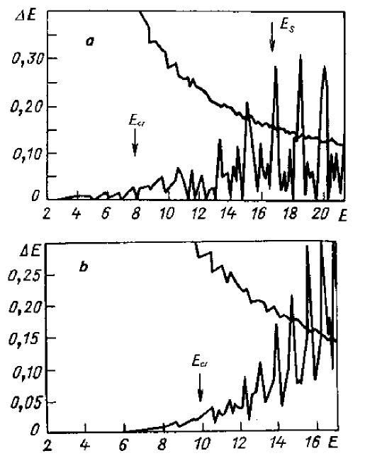
Figure 20: Difference between exact quantum energy levels and quasiclassical levels (22). The line is the mean level spacing. (a) for Henon-Heiles Hamiltonian with parameter $b=0.1$ $\left({E_{cr}=8.3;\;E_{S}=16.7}\right)$ ; (b) for Hamiltonian of quadrupole oscillations with parameters: $W=13;a=1;c=0.00135\left({E_{cr}=10}\right)$.

The dimension of submatrices of type $A_{1},A_{2},E$ are respectively equal $560,560$ and $415$ and provide sufficient precision of calculations for the first $250-300$ levels. The parameters of the Hamiltonian (16.1) are chosen so that $E_{cr1}=90$ . As it can be seen from the Table 3.3.1 in region, where classical motion is regular, the quantum normal form reproduces the energy spectrum with the relative error $\Delta E/E\sim 0.01\%$ . It seems naturally to expect that in the neighbourhood of critical energy of the transition to chaos, where the destruction of the approximate integrals of motion takes place and with the help of which the semiclassical spectrum is built, the agreement of the last one with the exact spectrum must essentially be getting worse. Let us analyze this effect on the example of the spectrum of quadrupole oscillations. The difference $\Delta E=\left|{E\left(M\right)-E_{ex}}\right|$ as the function of energy calculated for the case $W=13,E_{cr}=10$ is represented in Fig.20(b). We can see that in the region of energies, where the classical motion is regular, the approximate spectrum (22) reproduces the exact one rather well. At the transition to chaotic region the difference increases sharply. The similar situation takes place and for the Henon-Heiles Hamiltonian (Fig.20(a)).

1.4 $R-C-R$ transition and statistical properties of energy spectrum of the QON

Important correlations between peculiarities of classical dynamics and structure of quantum energy spectrum can be obtained in investigation of statistical properties of level sequences. We shall be interested in local properties of spectrum, i.e. in deviation in distribution of levels from mean values and in fluctuations. Why should we address to local characteristics of spectrum? The matter is, that the global characteristics like the numbers of states $N(E)$ or the smoothed density of levels $\rho(E)$ are too rough. At the same time, such local characteristics, as the function of the nearest-neighbour spacing distribution between levels is very sensitive to the properties of potential and to the shape of boundary. It is sufficient, for example, to bend slightly one of the walls in square to make it scattering, then classical trajectories in such system become chaotic. In this case the essential rearrangement of functions of the nearest-neighbour spacing distribution between levels happens, though the number of states $N(E)$ changes slightly or doesn’t change at all.

Relying on rather simple reasons [22], let’s try to construct one of the local characteristics of quantum spectrum - the function of the nearest-neighbour spacing distribution between levels $\rho(s)$ . For a random sequence the probability that a level will be in the small interval $(E+s,E+s+ds)$ , proportional, of course, to $ds$ , will be independent of whether or not there is a level at $E$ . This will be modified if we introduce level interaction. Given a level at $E$ , let the probability that the next level)$(s\neq 0)$ be in $(E+s,E+s+ds)$ be $P(s)ds$ . Then for $P(s)$ , the nearest-neighbour spacing distribution (NNSD), we have

$$P\left(S\right)dS=P\left({\left.{1\in dS}\right|0\in S}\right)P\left({0\in S}\right)$$ (24)

where $P(n\in S)$ is the probability that the interval of length $S$ contains $n$ levels and the $P(\left.{n\in dS}\right|m\in S)$ is conditional probability that the interval of length $dS$ contains $n$ levels, when that of length $S$ containes $m$ evels. The second factor in (24) is $\int\limits_{S}^{\infty}{P\left(x\right)dx}$ , the probability that the spacing is larger than $S$ , while the first one will be $dS$ times a function of $S,r_{10}(S)$ , depending explicitly on the choice, $1$ and $0$ , of the discrete variables $n,m$ . Then

$$P\left(S\right)=r_{10}\left(S\right)\int\limits_{S}^{\infty}{P\left(x\right)dx}$$ (25)

which we can solve easily to find

$$P\left(S\right)=cr_{10}\exp\left({-\int\limits_{0}^{S}{r_{10}\left(x\right)dx}}\right)$$ (26)

The Poisson law follows if we take $r_{10}(S)=1/D$ (the absence of correlations between level positions), where $D$ is the mean local spacing so that $1/D$ is the density of levels. Wigner’s law follows from the assumption of a linear repulsion, defined by $r_{10}(S)=\alpha S$ . The arbitrary constants are determined by conditions

$$\int{P\left(x\right)dx=1,}\int{xP\left(x\right)dx=D}$$ (27)

Finally, we find for the Poisson and Wigner cases, respectively

$$P\left(S\right)=1/D\exp\left({-{\raise 3.01385pt\hbox{$S$}\!\mathord{\left/{\vphantom{SD}}\right.\kern-1.2pt}\!\lower 3.01385pt\hbox{$D$}}}\right),\quad S\geqslant 0$$ (28)

$$P\left(S\right)=\frac{{\pi S}}{{2D^{2}}}\exp\left({-\frac{{\pi S^{2}}}{{4D^{2}}}}\right),\quad S\geqslant 0\quad$$ (29)

The second distribution displays the repulsion explicitly since $P\left(0\right)=0$ , in contrast to the Poisson form, which has a maximum at $S=0$ (level clusterization).

To get a first idea about origin of the level repulsion let us consider [22] the Hamiltonian as defined with respect to some fixed basis by its matrix elements. The repulsion may be regarded as arising from the fact that the subspace for which the corresponding spectrum has a degeneracy is of a dimensionality less by two than that of the general matrix-element space, so that in some sense a degeneracy is ”unlikely”. Alternatively [23], if we think of the matrix elements as functions of a parameter $\alpha$ , we cannot, in general, force a crossing by varying $\alpha$ but we must instead take the matrix elements as functions of at least two parameters which are independently varied. In the one-parameter case one will find that, if two levels approach each other as $\alpha$ is varied, then instead of crossing they will turn away as if repelled.

There is a principal difficulty with the derivation of (29). Why should we assume a linear repulsion? Although there are some plausibility arguments for this form, the result cannot be correct for every system. Furthermore only a probability arguments cannot explain the nature of level repulsion. However the situation changes, if we intend that statistical properties of the sequence of levels of real physical system are equivalent to the sequences of eigenvalues of the ensemble of random matrices of a definite symmetry. The theory, based on this hypothesis, was completed in the sixties [24], The final result for the function NNSD is

$$P\left(S\right)\approx S^{\alpha}\exp\left({-\beta S^{2}}\right)$$ (30)

The critical index $\alpha$ determining the behaviour of the distribution function at $S\to 0$ depends on the symmetry of the ensemble of matrices. This symmetry is determined by the properties of the physical system, the spectrum statistics of which we want to reproduce. If the system is invariant relative to time reversion, then the corresponding ensemble is Gaussian orthogonal ensemble (GOA). For the system assuming the violation of the invariance relative to time reversion the Gaussian unitary ensemble is associated. Finally, the symplectic ensemble of random matrices corresponds to the Hamiltonian of more complicated structure $H=H_{0}+\vec{h}\vec{\tau}$ , where $H_{0}^{*}=H_{0}^{T},h_{K}=h_{K}^{*}=-h_{K}^{T}$ , ($K=1,2,3;\;\sigma_{K}$ - Pauli matrices). The critical index $\alpha$ in the formula (30) is equal to: $\alpha=1$ for the GOA, $\alpha=2$ for the unitary ensembles and $\alpha=4$ for the symplectic ensembles.

The predictions of the statistical theory of levels (especially for the GOA) were compared in details with all available sets of nuclear data [22, 24]. No essential deviations between the theory and data base have been revealed. Similar comparisons have been realized for atomic spectra. And here, a good agreement has been revealed with the predictions of the GOA, though the number of processed data was essentially less, than in the nuclear spectroscopy.

If for the complicated systems (atomic nucleus, many-electron atom) we can give serious arguments in favour of the hypothesis of the equivalence of the statistical properties of the spectrum and the sequence eigenvalues of the ensemble of the random matrices, so its generalization does not seem natural in the case of the systems with a small number of degrees of freedom.

A radically new and sufficiently universal approach to the problem of the statistical properties of energy spectra may be developed on the basis of a nonlinear theory of dynamic systems. The numerical calculations [9, 25, 26, 27, 28], supported by sophisticated theoretical considerations [1, 3, 4, 9, 11, 13, 29, 30, 31], show that the important universal peculiarity of the energy spectra of the systems, that are chaotic in the classical limit, is the phenomenon of the level repulsion; while the systems, whose dynamics is regular in the classical limit, are characterized by the level clusterization. This statement is sometimes called [25] as the hypothesis of the universal character of the fluctuations of energy spectra.

Among the systems, which spectra were subjected to detail numerical analysis, the central place is occupied by two-dimensional billiards (free particle moving on the plane inside of some region and subjecting to elastic reflection on the boundary). One of two extremal situations can be realized for the billiards with the definite shape of the boundaries: integrable or nonintegrable. The angular momentum is the second integral (except energy) in the circular billiard and such a system is integrable. The billiard like ”stadium” is one of the simplest stochastic systems [67].

The NNSD for the integrable system (the circular billiard) is well approximated by Poisson distribution and the variance is the linear function of the considered energy interval, that is in complete correspondence with the hypothesis of the universal character of the fluctuations of energy spectra. In the nonintegrable case (”stadium”), the effect repulsion of levels and slow growth of the variance, caused by the rigidity of corresponding spectrum, are observed.

Measure of rigidity is the statistic $\Delta_{3}$ of Dyson and Mehta [32]

$$\Delta_{3}\left({L;x}\right)=\frac{1}{L}Min_{A,B}\int\limits_{x}^{x+L}{\left[{n\left(\varepsilon\right)-A\varepsilon-B}\right]^{2}dx}$$ (31)

which determines the least-square deviation of the staircase representing the cumulative density $n\left(\varepsilon\right)$ from the best straight line fitting it in any interval $\left[{x,x+L}\right]$ . The most perfectly rigid spectrum is the picket fence with all spacing equal (for instance, the one-dimensional harmonic oscillator spectrum),therefore maximally correlated, for which $\Delta_{3}(L)=1/12$ , whereas, at the opposite, the Poisson spectrum has a very large average value of $\Delta_{3}\left({\bar{\Delta}_{3}=L/15}\right)$ , reflecting strong fluctuations around the mean level density.

In contrast to billiards, where the character of motion does not depend on energy, the Hamiltonian systems of general position are the systems with the separable phase space, which contain both the regions, where the motion is stochastic, and the islands of stability. How is this circumstance reflected in statistical properties of spectrum? Berry and Robnik [30] and independently Bogomolny [33], basing on the semiclassical arguments, showed that NNSD for such system represents the independent superposition of the Poisson distribution with the relative weight $\mu$ , determining by the part of the phase space with regular motion, and the Wigner distribution with the relative weight $\bar{\mu}\left({\mu+\bar{\mu}=1}\right)$ , determining by the part of the phase space with chaotic motion

$$P\left(x\right)=\mu^{2}\exp\left({-\mu x}\right)erfc\left({\frac{{\sqrt{\pi}}}{2}\bar{\mu}x}\right)+\left({2\mu\bar{\mu}+\frac{\pi}{2}\bar{\mu}^{3}x}\right)\exp\left({-\mu x-\frac{\pi}{4}\bar{\mu}^{2}x^{2}}\right)$$ (32)

The expression (32) represents the interpolated formula between the Poisson (28) and Wigner (29) distributions.

Now let us go to the statistical properties of the spectrum of the Hamiltonian of the quadrupole oscillations (1). We intend to study the evolution of these properties in the process of $R-C-R$ transition, i.e. in each of energetic intervals $R_{1},\;C,\;R_{2}$ . In this study we are restricted by the case of one-well potentials ( $W<16$ ). At the fixed topology of potential surface ($W=const$ ) the unique free parameter of quantum Hamiltonian (1) is the scaled Planck’s constant $\bar{\hbar}i$ . In the study of the concrete energetic interval ($R_{1},C$ or $R_{2}$ ), corresponding to definite type of classical motion, the choice of $\bar{\hbar}_{i}$ is dictated by the possibility of attainment of the necessary statistical assurance (the required number of levels in investigated interval) with conservation of precision of spectrum calculation (restrictions to possibility of diagonalization of matrices of large dimension). Let us notice, that for the initial nonreduced Hamiltonian (16.1) the variation of $\bar{\hbar}_{i}$ is equivalent to the variation of the parameters $a;b;c$ (i.e. variation of the critical energies $E_{cr1}$ and $E_{cr2}$ ) or to the adequate choice of initial Planck’s constant $\bar{\hbar}_{i}\equiv\bar{\hbar}$ . The values of the scaled Planck’s constant $\bar{\hbar}_{3}\equiv\bar{\hbar}$ , represented in Table 3.4.1, allow us to obtain in corresponding energy intervals some hundreds of levels with the precision better than $1\%$.

Table 3.4.1

	$R_{1}$	$C$	$R_{2}$
$W=13$	$\bar{E}<8\cdot 10^{-5}$	$8\cdot 10^{-5}<\bar{E}<8.4\cdot 10^{-2}$	$\bar{E}>8.4\cdot 10^{-2}$
$\bar{\hbar}$	$\bar{\hbar}=3.2\cdot 10^{-6}$	$\bar{\hbar}=1.6\cdot 10^{-4}$	$\bar{\hbar}=1.1\cdot 10^{-1}$

Two additional comments are necessary before proceeding to results. We first recall that, to get rid of spurious effects of the local properties due to variation of the density, one has to work at constant density on the average. For this purpose one can ’unfold’ the original spectrum [22], i.e. map the spectrum of eigenvalues $\{E_{i}\}$ onto the spectrum $\left\{{\varepsilon_{i}}\right\}$ through

$$\varepsilon_{i}=\bar{N}\left({E_{i}}\right)$$ (33)

Here the smoothed cumulative density $\bar{N}\left(E\right)$ ,

$$\bar{N}\left(E\right)=\int\limits_{0}^{E}{\bar{\rho}\left({E^{\prime}}\right)dE^{\prime}}$$ (34)

and $\bar{\rho}\left(E\right)$ is the smoothed level density. In what follows we will take as energy unit the average spacing $\bar{x}$ between two adjacent levels of the unfolded spectrum

$$\bar{x}=\bar{s}_{i}=\left\langle{\left({\varepsilon_{i+1}-\varepsilon_{i}}\right)}\right\rangle$$ (35)

Meaning of unfolding is understood by the following example [34]. There are a few spacings between states of the same$(J^{\pi},T)$ in the ground state region known for many nuclei. Together they constitute a large sample of experimental spacing data. The only trouble is that the underlying scaling parameter $D$ varies from nucleus to nucleus. As a result, we cannot make statistical studies unless we have a model for the variation of $D$ as a function of nucleon number $A$ . This is a kind of unfolding except, instead of energy, we must remove the $A$ dependence of $D$ .

In the second place, we remark that our above discussion about Poisson of Wigner level statistics applies only for a pure sequence, i.e., one whose levels all have the same values of the exact quantum number. More precisely, a pure sequence represents a set of levels relating to one and the same nonreducible representation of the group of symmetry of considered Hamiltonian. In the case of mixed sequences [22] the level repulsion is moderated by the vanishing of Hamiltonian matrix elements connecting two different symmetry states, the spectra have moved towards random, and NNSD towards Poisson.

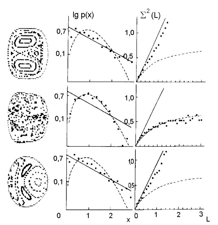
Figure 21: Correlation between the character of classical motion and statistical properties of energy spectra in $R-C-R$ transition for the Hamiltonian of quadrupole oscillations. On the left: - Poincare sections, in the middle - distribution function of the nearest-neighbour spacings, on the right - the variance. Below - the first regular range $\left({R_{1}}\right)$ , in the middle - the chaotic range, above - the second regular range $\left({R_{2}}\right)$ .

The results of investigation of correlations between statistical properties of energy spectrum of the Hamiltonian QON and the character of classical motion are represented in Fig.21 [35]. The typical Poincare surfaces of section, showing the change of classical regimes of motion, are represented at the left of Figure, and the statistical characteristics of spectrum (logarithm NNSD and dispersion), illustrating the evolution of the latter in the process of the $R-C-R$ transition, are represented at the right. At the construction of statistical characteristics, a purity of sequence is provided by using only those levels, which are relative to definite nonreducible representation of $C_{3v}$ group (the levels of $E$ -type were used for results represented in Fig.21; the statistical characteristics of levels of $A_{1}$ and $A_{2}$ - have similar form).

Both the NNSD and the variance well correspond to the predictions of GOE for the chaotic $(C)$ region . The logarithmic scale for NNSD $p(x)$ is suitable to trace this correspondence at large $x$ . For regular regions $R_{1}$ and $R_{2}$ the distribution function, in the same scale, according to the hypothesis of the universal character of fluctuations of energy spectra, must be represented by the straight line (the logarithm of Poisson’s distribution). The results demonstrate the agreement with this hypothesis, though not large deviations are observed for small distances between levels. Such a tendency to the rise of some repulsion in regular region, apparently, is connected with a small admixture of chaotic component.

The natural question about the role of numerical errors and, in particular, about the role of basis cutting off arises in careful studies of numerous examples confirming the hypothesis of the universal character of fluctuations of energy spectra. Even the special expression ”the induced nonregularity” has appeared [36]. The investigation of statistical properties of spectrum in three-levels model of Lipkin-Meshkov-Glick (LMG) [37] sheds a certain light on this problem.

Let us consider the system of $N$ particles on three levels, each of which is degenerated with multiplicity $N$ . The Hamiltonian of this system in representation of second quantization has the following form

$$H=\sum\limits_{k=0}^{2}{\varepsilon_{k}\left({\sum\limits_{n=1}^{N}{\alpha_{kn}^{+}\alpha_{kn}}}\right)}-\frac{1}{2}V\sum\limits_{k,l=0}^{n}{\left({1-\delta_{kl}}\right)\left({\sum\limits_{n=1}^{N}{\alpha_{kn}^{+}\alpha_{\ln}}}\right)}$$ (36)

where one-particle states (levels), marked by the indexes $k$ $(k=0,1,2)$ , and $n=1,2,...N$ are different degenerate states belonging to one level,$\alpha^{+},\alpha$ are fermionic creation and annihilation operators that obey the usual anticommutation relations.

More traditional two-levels model LMG [38] has unique degree of freedom (it is the number of particles on top level) and consequently its classical analog does not assume chaotic behaviour. Introduction of an additional level is equivalent to the appearance of additional degree of freedom. Stationary states of the Hamiltonian (36) can be marked by two indexes - the numbers of particles on the second and the third levels. As there is the finite number of ways of distribution of $N$ particles on three levels, then the number of basis vectors in this model is finite. The problems of basis cutting off and estimation of arising errors are absent.

Using coherent states

$$\left|z\right\rangle=\exp\left({\sum\limits_{k=1}^{2}{\sum\limits_{n=1}^{N}{z_{k}\alpha_{kn}^{+}\alpha_{0n}}}}\right)\left|0\right\rangle$$ (37)

where $\left|0\right\rangle$ is the state with all $N$ particles on level with $k=0$ , we determine the classical Hamiltonian $H_{cl}$ as

$$\begin{gathered}H_{cl}\equiv\frac{1}{{N\varepsilon}}\left\langle z\right|H\left|z\right\rangle=-1+\frac{1}{2}q_{1}^{2}\left({1-\chi}\right)+\frac{1}{2}q_{2}^{2}\left({2-\chi}\right)+\frac{1}{2}p_{1}^{2}\left({1+\chi}\right)+\frac{1}{2}p_{2}^{2}\left({2+\chi}\right)+\hfill\\ +\frac{\chi}{4}\left[{\left({q_{1}^{2}+q_{2}^{2}}\right)^{2}-\left({p_{1}^{2}+p_{2}^{2}}\right)^{2}-\left({q_{1}^{2}-p_{1}^{2}}\right)\left({q_{2}^{2}-p_{2}^{2}}\right)-4q_{1}q_{2}p_{1}p_{2}}\right]\hfill\\ \end{gathered}$$ (38)

Here $\chi$ is the distance between levels, $\chi=(N-1)^{V}/\varepsilon$ ,

$$q_{k}=\operatorname{Re}\frac{{\sqrt{2}z_{k}}}{{\sqrt{1+\left|{z_{1}}\right|^{2}+\left|{z_{2}}\right|^{2}}}},p_{k}=\operatorname{Im}\frac{{\sqrt{2}z_{k}}}{{\sqrt{1+\left|{z_{1}}\right|^{2}+\left|{z_{2}}\right|^{2}}}}$$ (39)

The equations of motion for $q_{k}$ and $p_{k}$ , obtained from variational principle [5] are Hamiltonian. The classical analog of the Hamiltonian LMG is integrable at $\chi=0\;(V=0)$ . Changing the value of the constant of connection $\chi$ we can observe the transition from regular motion to chaotic one. The spectral fluctuations for three-levels model LMG given in Fig.22. These results are the serious argument in favour of the hypothesis of the universal character of fluctuations of energy spectra.

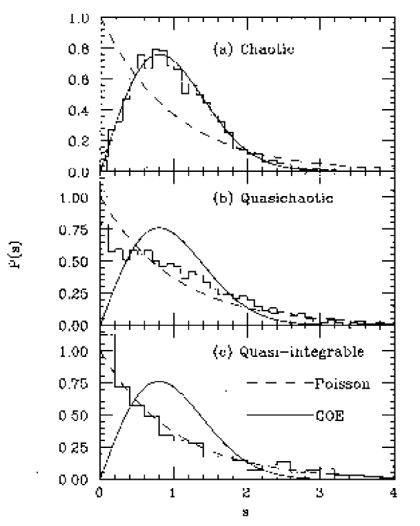
Figure 22: The spectral fluctuations in three-levels model LMG: a - distribution function of the nearest-neighbour spacings, b - the variance [81].

1.5 $R-C-R$ transition and the structure of QON wave function

As we have seen in the previous section, the statistical properties of quantum spectrum of the Hamiltonian QON have been rigidly correlated with the type of classical motion. It is naturally to try to discover the analogous correlations in the structure of wave functions, i.e. to assume, that the form of the wave function for a semiclassical quantum state, associated with classical regular motion in the regions $R_{1}$ or $R_{2}$ , is different from the one for chaotic region $C$ . Notice that in contrast to the description of the energy spectra where we now have a sufficiently complete understanding of the spectral statistical properties we are still far from a corresponding complete knowledge of generic structure properties of the wave functions. Furthermore it should be pointed out that in analysis of QMCS at the level of energy spectra the principal role was given to statistical characteristics, i.e., the quantum chaos was treated as a property of the group states. The choice of a stationary wave function of the quantum system, which is chaotic in the classical limit, as an basic object of investigation relates the phenomenon of quantum chaos to an individual state.

In contrast to spectrum the form of wave functions depends on the basis in what they are determined. Studying QMCS the three following representations are used more often

1. The so called $H_{0}$ -representation is: the representation of eigenfunctions $\left\{{\varphi_{n}}\right\}$ of integrable part $H_{0}$ of total Hamiltonian $H=H_{0}+V$ . The main objects of investigation in this case are the coefficients of expansion $C_{mn}$ of stationary functions $\psi_{m}$ in basis $\left\{{\varphi_{n}}\right\}$ . $H_{0}$ -representation is natural at realization of numerical calculations, as diagonalization of Hamiltonian $H$ is realized more often just in this representation.

2. Coordinate representation in which the behaviour of wave functions simply allows visual comparison with the picture of classical trajectories in coordinate space.

3. Representation with the help of Wigner’s functions [39] has a set of properties, common with classical function of distribution in phase space.

As early as 1977 Berry [40] assumed, that the form of the wave function $\psi$ for a semiclassical regular quantum state (associated with classical motion on a $N$ -dimensional torus in the $2N$ -dimensional phase space) was very different from the form of $\psi$ for an irregular state (associated with stochastic classical motion on all or part of the $\left({2N-1}\right)$ -dimensional energy surface in phase space). For the regular wave functions the average probability density in the configuration space was seen to be determined by the projection of the corresponding quantized invariant torus onto the configuration space, which implies the global order. The local structure is implied by the fact that the wave function is locally a superposition of a finite number of plane waves with the same wave number as determined by the classical momentum. In the opposite case for the chaotic wave functions the averaged (over small intervals of energy and coordinates) square of the eigenfunctions in the semiclassical limit $\hbar\to 0$ coincides with the projection of the classical microcanonical distribution to the coordinate space. Its local structure is spanned by the superposition of infinitely many plane waves with random phases and equal wave numbers. The random phases might be justified by the classical ergodicity and this assumption immediately predicts locally the Gaussian randomness for the probability of amplitude distribution. Such structure of wave function is in well agreement with the picture of classical phase space: the classical trajectory homogeneously fill isoenergetic surface in condition corresponding to chaotic motion. By contrast, from the consideration of regular quantum state as analog of classical motion on torus, a conclusion should be done about the singularity (in limit $\hbar\to 0$ ) of wave function near caustics (boundaries of region of classical motion in coordinate space).

Berry’s hypothesis was subjected to the most complete test for billiards of different types and, in particular, for billiard stadium type [41]. The amplitude of typical wave function of integrable circular billiard is negligible in classical prohibited region (from conservation of angular moment in circular billiard it should be that the arbitrary trajectory is enclosed between external and certain internal circle, the radius of which is determined by the angular moment) , whereas near the caustics it is maximal. Distribution $\left|\psi\right|^{2}$ for the case stadium, at which classical dynamics is stochastic, is strongly distinguished from the integrable case. However, this distribution is not so homogeneous, as we could expect starting from the ergodicity of classical motion.

Investigating QMCS in connection with properties of wave functions let us pass from billiards to Hamiltonian system of general position [42, 43]. For this purpose let us return to the object of our investigation: $C_{3v}$ symmetric Hamiltonian QON. We begin to study the correlations of our interest by the topography of level curves of the stationary wave functions and, in particular, of nodal curves on which $\psi_{k}(x,y)=0$ . One of a nonrigorous criterion of stochasticity [44] states that the system of nodal curves of regular wave function is a lattice of quasiortogonal curves or is similar to such a lattice. At the same time, the wave functions of chaotic states do not have such a representation. Fig.23 confirms that the structure of the lattice of nodal curves of separable wave functions undergoes a change in the $R-C-R$ transition. The spatial structure of nodal curves for states from regions $R_{1}$ and $R_{2}$ of regular classical motion is considerably simpler than this structure for states from region $C$ of chaos.

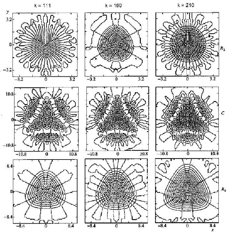
Figure 23: Nodal curves of the wave functions $\psi_{k}\left({x,y}\right)$ . The numbers $k$ of the corresponding levels are shown over the figures.

Correlations between the structure of wave function and the type of classical motion are also demonstrated in Fig.24, in which the probability density $\left|{\psi\left({x,y}\right)}\right|^{2}$ for states with numbers $111,160$ and $210$ is represented. The squared module of the wave functions reproduces rather well transition from functions with clear internal structure (region $R_{1}$ ) to an irregular distribution (region $C$ ) and the restoration of structure in the second regular region ($R_{2}$ ). For the chosen technique, in which transition is traced for the wave function with fixed number (because of our use of the scaled Planck constant), a change in the wave function is associated only with $R-C-R$ transition.

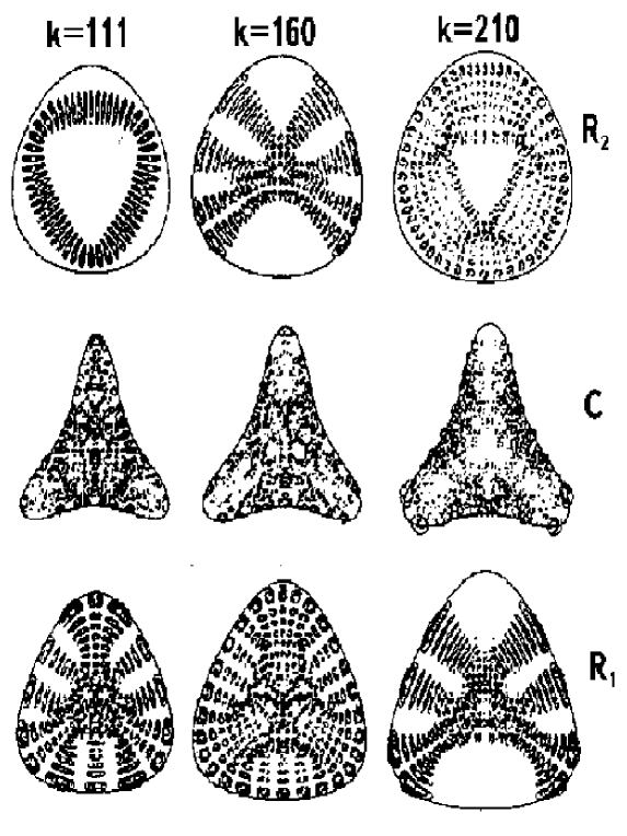
Figure 24: Isolines of probability density $\left|{\psi_{k}\left({x,y}\right)}\right|^{2}$ . The step between isolines is constant. The numbers $k$ of the corresponding levels are shown over the figures.

Evolution of the wave functions in the process of $R-C-R$ transition can be studied also in $H_{0}$ -representation or more exactly in the representation of linear combinations of wave functions of two-dimensional harmonic oscillator with equal frequencies (see Section 3.2)

$$\Psi_{k}=\sum\limits_{N,L}{C_{NLj}^{k}\left|{NLj}\right\rangle}$$ (40)

If one introduces the notion of distributivity of wave function in basis, then the criterion of stochasticity formulated by Nordholm and Rise [45] even in 1974 states that with the degree of stochastization in the average arises the degree of distributivity of wave functions. It is clear that this criterion is a direct analog of the Berry’s hypothesis for $H_{0}$ - representation, if one interprets the number of basis state $i=\left\{{NLj}\right\}$ as a discrete coordinate. Fig.25 qualitatively confirm validity of this criterion. It can be seen from this figure that the states that correspond to regular motion are distributed in a relatively small number of basis states. At the same time, states corresponding to chaotic motion (region $C$ ) are distributed in a considerably larger number of basis state. In the latter case, the contributions from a large number of basis states in expansion (40) interfere; this results in a complex spatial structure of the wave function $\psi_{k}\left({x,y}\right)$ .

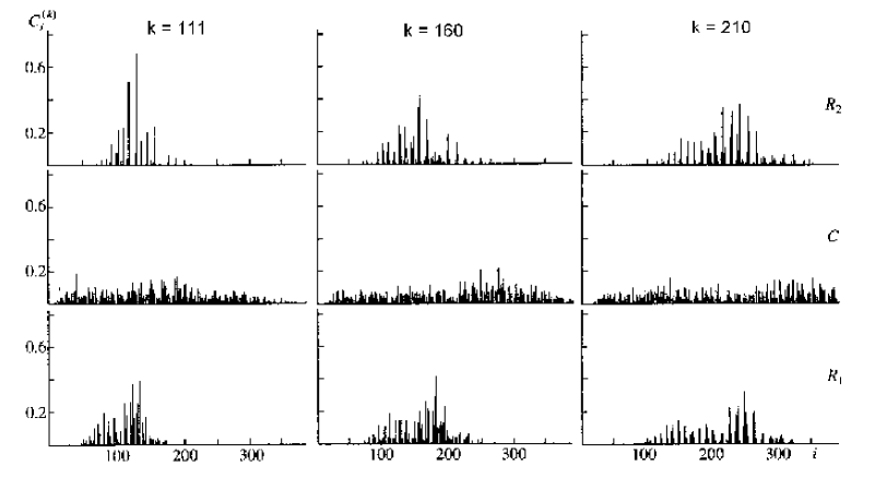
Figure 25: Distribution of the coefficient $C_{i}^{\left(k\right)}$ in the number $i=\left\{{N,L,j}\right\}$ of the basis state. The numbers $k$ of the corresponding levels are shown over the figures.

For quantitative estimation of a degree of distributivity of wave functions, it is useful to introduce [46, 47] the analog of usual thermodynamic entropy

$$S^{k}=-\sum{\left|{C_{NLj}^{k}}\right|^{2}\ln\left|{C_{NLj}^{k}}\right|^{2}}$$ (41)

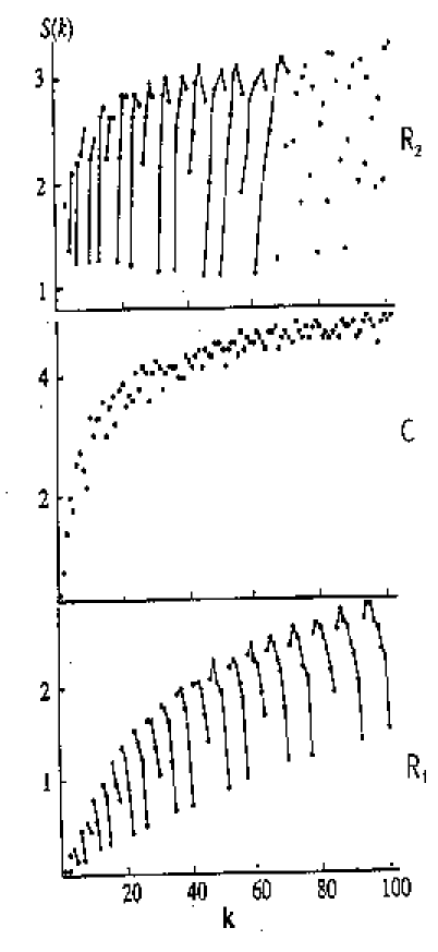
Figure 26: Entropy $S$ as a function of the state number. The stright lines connecting the points correspond to shell classification according to $N$ .

Fig.26 represents the dependence of entropy $S$ from the number of state k for the first regular $\left({R_{1}}\right)$ and chaotic $\left(C\right)$ regions. From this figure we can see, that the type of classical motion in large measure determines the character of this dependence: in chaotic region the entropy is practically constant, that corresponds to the high degree of distributivity, and in regular region the entropy is less in the value and has nonmonotone character. Nonmonotonicity of $S$ is connected with rather high degree of localization of the wave function depending on the number of state. This effect and also the behaviour of the entropy in the second regular region $R_{2}$ , will be studied in detail in the following section.

1.6 Evolution of shell structure in the process of $R-C-R$ transition

In sections 3.4 and 3.5 we have studied the change of statistical roperties of energy spectra and structure of wave functions in the process of $R-C-R$ transition. However, the utility of the concept of the stochasticity extends further. Introduction of this concept in the nuclear theory made possible to take a fresh look [7] at the old paradox [8]: how one could reconcile the liquid drop - short mean free path - model of the nucleus with the independent particles - gas - like shell model. For the solution of this paradox within the limits of philosophy of simple chaos (see section 1.1(part 1)) it is sufficient to assume [7]

1) When the nucleonic motion inside the nucleus is integrable, one expects to see strong shell effects in nuclear structure, quite well reproducible, for example, by the model of independent particles in the potential well.

2) When nucleonic motion is chaotic, one expects smooth, statistical, Thomas-Fermi, Droplet model approaches to be good approximations. This is because phase space is much more uniformly filled with the Boltzmann fog in this case. At such approach the elucidation of the mechanism of destruction of shell effects in the process of the transition regularity-chaos plays the key role. More appropriately the problem can be formulated in the following way [7]: how do shell dissolve with deviations from integrability or, conversely, how do incipient shell effects emerge as the system first begins to feel its proximity to an integrable situation?

As it has been mentioned many times, the finite motion of integrable Hamiltonian system with $N$ -degrees of freedom is, in general, conditionally periodic, and the phase trajectories lie on $N$ -dimensional tori. In the variables action-angle $\left({I,\theta}\right)$ the Hamiltonian is cyclic with respect to angle variables, $H=H_{0}\left(I\right)$ . Even at the beginning of the century, Poincare called the main problem of dynamics the problem about the perturbation of conditionally periodic motion in the system defined by the Hamiltonian

$$H=H_{0}\left(I\right)+\varepsilon V\left({I,\theta}\right)$$ (42)

where $\varepsilon$ is a small parameter. The essential step in the solution of this problem was the KAM theorem, asserting, that at switching on nonintegrable perturbation, the majority of nonresonance tori, i.e. the tori for which

$$\sum\limits_{i=1}^{N}{n_{i}\frac{{\partial H_{0}}}{{\partial I_{k}}}\neq 0}$$ (43)

is conserved, distinguishing from the nonperturbed cases only by small (to the extent of smallness of $\varepsilon$ ) deformation. As we have seen in section 2.3(part 1), at definite conditions the KAM formalism allows to remove out of Hamiltonian the members depending on angle, using the convergent sequence of canonical transformations [2]. When it is succeed, we immediately find that perturbed motion lies on rather deformed tori so that trajectories, generated by perturbed Hamiltonian, remain quasiperiodic. In other words the KAM theorem reflects an important peculiarity of classical integrable systems to conserve regular behaviour even at rather strong nonintegrable perturbation. In the problem of our interest, concerning the destruction of shell structure of quantum spectrum, the KAM theorem also will be able to play an important role. Considering the residual nucleon-nucleon interaction as nonintegrable addition to selfconsistent field, obtained, for example, in Hartree-Fock approximation, one can try to connect the destruction of shell with the deviation from integrability. The existence of shell structure at rather strong residual interaction (or at large deformation) can be obligated to rigidity of KAM tori, contributing to survival of regular behaviour. Such assumption seems rather natural, especially if one takes into account, that the procedure of quasiclassical quantization itself [48, 49] is indirectly based on convergence of the same sequence of canonical transformations, as the KAM theorem.

The aim of this section is to trace the evolution of the structure of QON Hamiltonian. In numerical calculations of this section it will be more convenient for us to use nonscale version of the Hamiltonian (16.1). By nonperturbed Hamiltonian $H_{0}$ we will mean the Hamiltonian of two-dimensional harmonic oscillator with equal frequencies: $H_{0}\equiv H\left({a=1,b=0,c=0}\right)$ . Its degenerate equidistant spectrum is well known. At switching on perturbation, the degeneration disappears and the shell structure forms. The number of states, for example, the states of $E$ - type (the numerical results, represented below, are relative to the states precisely of this type, though analogous results take place for the states belonging to another nonreducible representations of $C_{3v}$ - group) for the given quantum number $N$ is equal to $\frac{1}{2}\left({N_{1}+Mod\left({N,2}\right)}\right)$ , where $N_{1}=\frac{1}{3}\left({2N+Mod\left({N,3}\right)}\right)$ , and $Mod\left({N,M}\right)$ is a remainder from division of $N$ by $M$ .

It is obvious, that eigenfunctions of exact Hamiltonian QON are not the eigenfunctions of operators $\hat{N}$ and $\hat{L}$ already. Nevertheless, as numerical calculations show even at rather large nonlinearity, one can use the quantum number $N$ and $L$ for the classification of wave functions. The measure of nonlinearity, at which such classification (i.e. the existence of shell structure) remains reasonable, is connected with quasicrossing of neighbouring levels. Under the quasicrossing we shall understand the approach of levels up to the distances of degree of precision of numerical calculations (the detailed analysis of quasicrossing see lower).

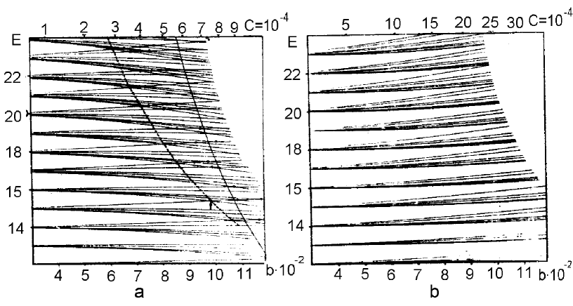
Figure 27: a. Energy spectra of Hamiltonian (16.1) depending on values of parameter $b$ for region $C$ $\left({W=13}\right)$ . Points mark quasicrossinds. Continuous line - dependence $E_{cr}$ from $b$ . Dashed line shows the beginning of the region of quasicrossings. Arrow shows point of quasicrossing of the levels with $k=40$ and $41$ . b. Energy spectra of Hamiltonian (16.1) depending on values of parameter $b$ for region $R_{1}\left({W=3.9}\right)$ . There are no quasicrossing of the levels.

The dependence of energy spectra of Hamiltonian QON from the parameter $b$ for the values $W=3.9$ and $W=13$ are represented in Fig.27a,b. As it is seen from Fig. 27a. for the PES with $W=13$ at the approaching to the line of critical energy of the transition to chaos, defined according to the criterion of negative curvature, the destruction of shell structure, which we understand as multiple beginning of quasicrossing, takes place. At the same time, for the PES with $W=3.9$ in Fig.27b (for which as we have shown in Section 2.4(part 1), the local instability is absent and the motion is regular at all energies) the quasicrossings are absent even at larger nonlinearity than in Fig.27a for $W=13$ .

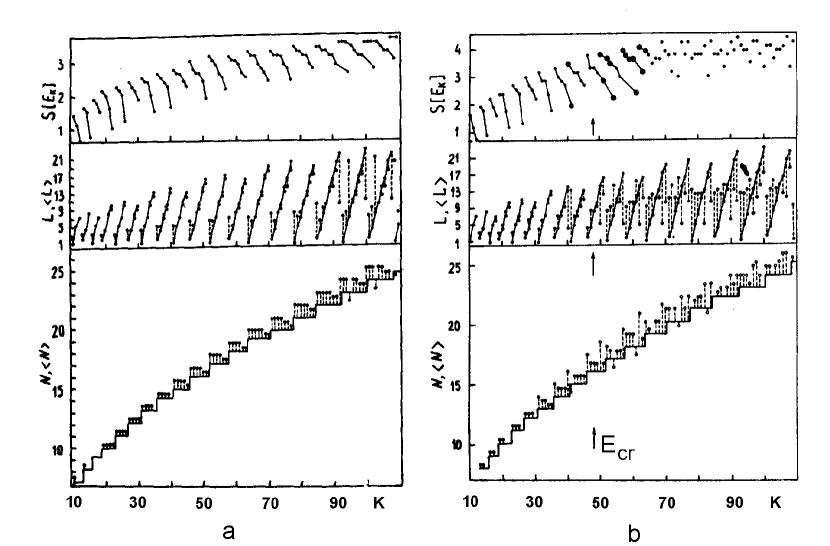
Figure 28: Entropy $S$ and quantum numbers $L$,$N$ as the functions of state number $k$.

The destruction of shell structure can be traced for the wave functions, using introduced in previous section, the analog of thermodynamic entropy $S\left({E_{k}}\right)$ . The character of changes of entropy in regions $R_{1}$ and $R_{2}$ , corresponding to regular classical motion, correlates with the transition from shell to shell (see Fig.28). Two effects are observed in the region $C$ , corresponding to chaotic classical motion. Firstly, quasiperiodical dependence of entropy from energy is violated, that testifies to destruction of sell structure. Secondly, the monotone growth of entropy is observed on average with going out on plateau corresponding to the entropy of random sequence at the energies essentially exceeding critical energy.

Average values of operator $\hat{N}$ , given in Fig. 29, and calculated on stationary wave functions of exact Hamiltonian, describe the dynamics of change of the shell structure. From this Figure we can see, that the minimum deviation of $\left\langle N\right\rangle$ from $N$ is observed in regions $R_{1}$ and $R_{2}$ , while this deviation is considerably greater in the stochastic region $C$ ; moreover in the average it monotonically increases with increase of energy. It is obvious, that at energies, for which $N-\left\langle N\right\rangle\geqslant 1$ , the destruction of quantum analogs of classical integrals leads to the fact that the classification of levels with the help of quantum numbers $N$ and $L$ loses sense.

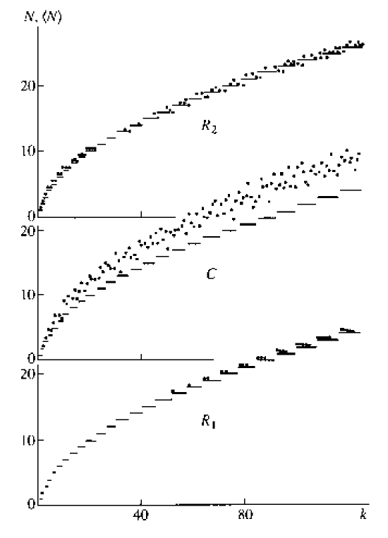
Figure 29: Dependence of $N$ (lines) and $\left\langle N\right\rangle$ points) of state numbers $k$ .

Notice, that we could observe restoration of shell structure at high energies in the process of $R-C$ transition only due to the optimization of basis frequency (see Section 1.2), that is equivalent to the possibility of diagonalization of matrices of considerably higher dimension.

Now let us return to the analysis of quasicrossings of levels arising near critical energy of the transition to chaos. As it is known [50], for the set of Hamiltonians depending on two parameters $\lambda=\left({b,c}\right)$ and that is invariant with respect to inversion of time in the neighbourhood of degeneration point $\lambda^{*}=\left({b^{*},c^{*}}\right)$ , the difference of two terms $\Delta E=E_{1}-E_{2}$ is determined by the expression

$$\Delta E\left({b,c}\right)=\left[{A\left({b-b*}\right)^{2}+B\left({b-b*}\right)\left({c-c*}\right)+C\left({c-c*}\right)^{2}}\right]^{{\raise 2.1097pt\hbox{$1$}\!\mathord{\left/{\vphantom{12}}\right.\kern-1.2pt}\!\lower 2.1097pt\hbox{$2$}}}$$ (44)

where coefficients $A,B,C$ are the functions of components $\nabla_{\lambda}H$ in the point $\lambda^{*}$ . The characteristics of nuclear shape [48] in the problems of nuclear spectroscopy more often play the role of parameters. The wave functions of intersecting levels near degeneration point can be represented in the following form

$$\begin{gathered}\left|{E_{1}\left(\lambda\right)}\right\rangle=\cos\chi_{1}\left|{E_{1}\left({\lambda^{*}}\right)}\right\rangle+\sin\chi_{1}\left|{E_{2}\left({\lambda^{*}}\right)}\right\rangle\hfill\\ \left|{E_{2}\left(\lambda\right)}\right\rangle=\cos\chi_{2}\left|{E_{1}\left({\lambda^{*}}\right)}\right\rangle+\sin\chi_{2}\left|{E_{2}\left({\lambda^{*}}\right)}\right\rangle\hfill\\ \end{gathered}$$ (45)

where angles of mixing $\chi_{1,2}$ are determined by the relation

$$\begin{gathered}e^{2i\chi_{1,2}}=\pm\frac{{\left({T\lambda}\right)+i\left({S\lambda}\right)}}{{\left[{\left({T\lambda}\right)^{2}+\left({S\lambda}\right)^{2}}\right]^{{\raise 2.1097pt\hbox{$1$}\!\mathord{\left/{\vphantom{12}}\right.\kern-1.2pt}\!\lower 2.1097pt\hbox{$2$}}}}},\hfill\\ \left({T\lambda}\right)\approx H_{11}\left(\lambda\right)-H_{22}\left(\lambda\right),\left({S\lambda}\right)\approx 2H_{21}\left(\lambda\right)\hfill\\ \end{gathered}$$ (46)

It is easy to see, that changing $\lambda\to-\lambda$ the ”exchange” of wave functions of approaching levels takes place $\left|{E_{1}\left({\lambda*}\right)}\right\rangle\leftrightarrow\left|{E_{2}\left({\lambda*}\right)}\right\rangle$ . Such test can be effectively used for the analysis of nature of quasicrossing points.

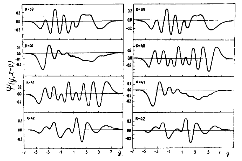
Figure 30: Wave functions $\psi\left({x=0,y}\right)$ for the states with $k=39,40,41,42$ in the neighbourhood of quasicrossing of the states with $k=40$ and $41$ . Left $b<b^{*}$ , right $b>b^{*}$ (point of quasicrossing: $b^{*}=0.098;\;c^{*}=0.00074$ ).

We trace, in particular, the variations of functions with $K=40$ and $K=41$ , which undergo quasicrossing in the neighbourhood $b^{*}\approx 9.8\cdot\;10^{-2},\quad c^{*}\approx 7.4\cdot 10^{-4}$ (recall, that under this term we understand the approaching of levels up to distances of an order of precision of numerical calculations). The sections of $\Psi(x=0,y)$ and coefficients of expansions $C_{NLj}^{k}$ of wave functions of considering states before and after quasicrossing point are represented in Figs 30 and 31. The similar characteristics of the states with $K=39$ and $K=42$ which do not undergo quasicrossing at this values of parameters are represented for comparison at the same figure.

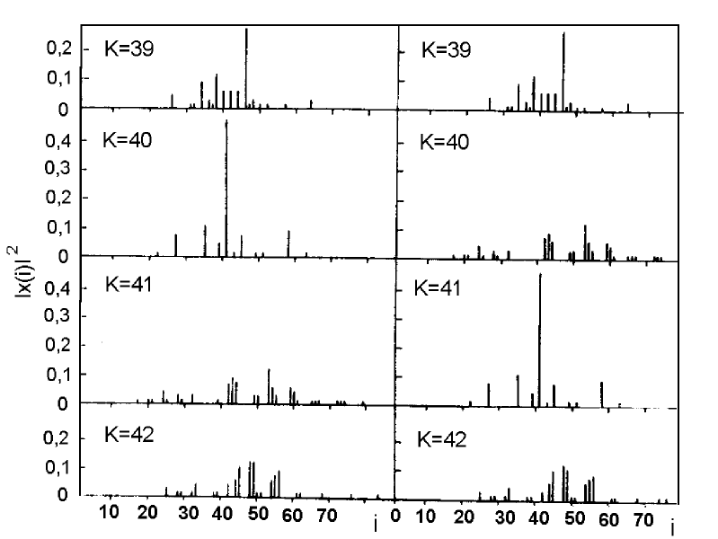
Figure 31: Same as Figure 30, but for the coefficients of the expansion of wave functions $\left|{x\left(i\right)}\right|^{2}=\left|{C_{NLj}^{\left(k\right)}}\right|,\;i$ , - number of basis state.

As it is seen in represented figures the wave functions are not practically changed for the states 39 and 42, at the same time the exchange of wave functions is observed for the states $40$ and $41$ in correspondence with test described above. Analogous situation takes place for other quasicrossings .

1.7 Wave packet dynamics

The investigation of the time evolution of nonstationary states, i.e. of packets in quantum systems classical analogs of which admit chaotic behaviour, gives an important information about QMCS. The localized quantum wave packet (QWP) is the closest analog of the point in phase space, which describes the state of classical system. However, the correspondence between localized QWP and classical point particle in chaotic region is broken down in a very short time interval. Let us explain it by using Takahashi arguments [52]. We take two localized QWP $\Psi_{1}\left(x\right)$ and $\Psi_{2}\left(x\right)$ which are put in the chaotic region at initial time to be slightly different from each other so that the difference between $\left\langle{\Psi_{1}}\right|\hat{x}\left|{\Psi_{1}}\right\rangle$ and $\left\langle{\Psi_{2}}\right|\hat{x}\left|{\Psi_{2}}\right\rangle$ (or $\left\langle{\Psi_{1}}\right|\hat{p}\left|{\Psi_{1}}\right\rangle$ and $\left\langle{\Psi_{2}}\right|\hat{p}\left|{\Psi_{2}}\right\rangle$ ) is very small. We assume that in chaotic region the localized QWP does not either extend in a certain time interval of the order ${\raise 3.01385pt\hbox{$1$}\!\mathord{\left/{\vphantom{1{\sqrt{\hbar}}}}\right.\kern-1.2pt}\!\lower 3.01385pt\hbox{${\sqrt{\hbar}}$}}$ like that in regular region. Thence, following the Ehrenfest theorem, the packets $\Psi_{1}$ and $\Psi_{2}$ move as classical particles and the distance between $\left\langle{\Psi_{1}}\right|\hat{x}\left|{\Psi_{1}}\right\rangle$ and $\left\langle{\Psi_{2}}\right|\hat{x}\left|{\Psi_{2}}\right\rangle$ (or $\left\langle{\Psi_{1}}\right|\hat{p}\left|{\Psi_{1}}\right\rangle$ and $\left\langle{\Psi_{2}}\right|\hat{p}\left|{\Psi_{2}}\right\rangle$ ) is increasing exponentially in time. Let us consider the superposition $\Psi=\Psi_{1}+\Psi_{2}$ which also becomes a localized QWP in initial state. From the assumption, we can expect that QWP $\Psi$ does not extend in a certain time interval of the order ${\raise 3.01385pt\hbox{$1$}\!\mathord{\left/{\vphantom{1{\sqrt{\hbar}}}}\right.\kern-1.2pt}\!\lower 3.01385pt\hbox{${\sqrt{\hbar}}$}}$ . However, considering the exponential increment of the distance between $\left\langle{\Psi_{1}}\right|\hat{x}\left|{\Psi_{1}}\right\rangle$ and $\left\langle{\Psi_{2}}\right|\hat{x}\left|{\Psi_{2}}\right\rangle$ , $\Psi$ extends exponentially in chaotic region and does not behave as a classical particle. This result is inconsistent with initial assumption and implies that in chaotic region the localized QWPs (i.e. $\Psi_{1}$ , $\Psi_{2}$ and $\Psi$ ) extend exponentially like a classical probability distribution in the first stage of time development.

In order to describe such unusual behaviour of QWP one should address to the concept of a quantum-mechanical phase space. There are a few well-established schemes to introduce phase-space variables in quantum mechanics [39, 53, 54, 55]. In the present study we shall follow the procedure proposed by Weissman and Jortner [56]. Let us consider an initially localized QWP $\Psi$ characterized by the coordinates $q$ and the momenta $p$ ,

$$\begin{gathered}q=\left\langle\Psi\right|\hat{q}\left|\Psi\right\rangle\hfill\\ p=\left\langle\Psi\right|\hat{p}\left|\Psi\right\rangle\hfill\\ \end{gathered}$$ (47)

Now we introduce the coherent states $\left|{p,q}\right\rangle$ [54], which in the coordinate x-representation, are given by Gaussian wave packets

$$\left\langle{x}\mathrel{\left|{\vphantom{x{p,q}}}\right.\kern-1.2pt}{{p,q}}\right\rangle=\prod\limits_{j=1}^{N}{\left({\pi\sigma_{j}^{2}}\right)^{-{\raise 2.1097pt\hbox{$1$}\!\mathord{\left/{\vphantom{14}}\right.\kern-1.2pt}\!\lower 2.1097pt\hbox{$4$}}}\exp\left[{-\frac{{\left({x_{j}-q_{j}}\right)^{2}}}{{2\sigma_{j}^{2}}}+\frac{{ip_{j}x_{j}}}{\hbar}-\frac{{ip_{j}q_{j}}}{{2\hbar}}}\right]}$$ (48)

In the study of a system of $N$ coupled harmonic oscillators, it is convenient to choose for constants $\sigma_{j}$ the rms zero-point displacements

$$\sigma_{j}=\left({{\raise 3.01385pt\hbox{$\hbar$}\!\mathord{\left/{\vphantom{\hbar{m_{j}\omega_{j}}}}\right.\kern-1.2pt}\!\lower 3.01385pt\hbox{${m_{j}\omega_{j}}$}}}\right)^{{\raise 2.1097pt\hbox{$1$}\!\mathord{\left/{\vphantom{12}}\right.\kern-1.2pt}\!\lower 2.1097pt\hbox{$2$}}}$$ (49)

where mj are masses and $\omega_{j}$ are frequencies of the uncoupled oscillators. With this choice of the $\sigma_{j}$ , the coherent states $\left|\alpha\right\rangle\equiv\left|{p,q}\right\rangle$ become the eigenstates of the harmonic oscillator annihilation operators $a_{j}$

$$a_{j}\left|\alpha\right\rangle=\alpha_{j}\left|\alpha\right\rangle$$ (50)

where a complex variable $\alpha_{j}$ ,

$$\alpha_{j}=\frac{1}{{\sqrt{2}}}\left({\frac{{q_{j}}}{{\sigma_{j}}}+i\frac{{\sigma_{j}}}{\hbar}p_{j}}\right)$$ (51)

Using these coherent states, it is possible to introduce the following quantum - mechanical phase-space density

$$\rho_{\Psi}\left({q,p}\right)=\left|{\left\langle{\alpha}\mathrel{\left|{\vphantom{\alpha\Psi}}\right.\kern-1.2pt}{\Psi}\right\rangle}\right|^{2}$$ (52)

where $\Psi$ is any general wave packet. This quantum-mechanical, coherent-state, phase-space density may be regarded as a quantum analog of the classical phase-space density, since it satisfies an equation of motion whose leading term (when expanded in powers of $\hbar$ ), corresponds to the classical Liuville equation [66]. The stationary phase space densities $\rho_{E}\left({p,q}\right)$ are the squares of the projections of the eigenstates on the coherent state,

$$\rho_{E}\left({p,q}\right)=\left|{\left\langle{\alpha}\mathrel{\left|{\vphantom{\alpha E}}\right.\kern-1.2pt}{E}\right\rangle}\right|^{2}$$ (53)

where $\left|\alpha\right\rangle$ is given in terms of Gaussian wave packet (48) while the eigenstate $\left|E\right\rangle$ is given by Eq.(4). Using the well-known expressions for scalar products $\left\langle{\alpha}\mathrel{\left|{\vphantom{\alpha{NL}}}\right.\kern-1.2pt}{{NL}}\right\rangle$ [54] we finally obtain

$$\begin{gathered}\rho_{E}\left({p,q}\right)=\frac{1}{2}\exp\left[{-\frac{1}{2}\left({\left|{\alpha_{+}}\right|^{2}+\left|{\alpha_{-}}\right|^{2}}\right)}\right]\cdot\hfill\\ \times\sum\limits_{N,L}{\frac{{C_{NL}}}{{\left({n_{-}!\;n_{+}!}\right)^{{\raise 2.1097pt\hbox{$1$}\!\mathord{\left/{\vphantom{12}}\right.\kern-1.2pt}\!\lower 2.1097pt\hbox{$2$}}}}}\left({\alpha_{+}^{*n_{+}\;}\alpha_{-}^{*n_{-}}+\;j\;\alpha_{+}^{*n_{-}}\alpha_{-}^{*n_{+}}}\right)\;}\hfill\\ \end{gathered}$$ (54)

where $\alpha_{\pm}=\frac{1}{{\sqrt{2}}}\left({\alpha_{2}\mp i\alpha_{1}}\right)$ with $\alpha_{1,2}=\frac{1}{{\sqrt{2}}}\left({q_{1,2}+ip_{1,2}}\right)$ , $n_{+}=\frac{{N+L}}{2}$ , $n_{-}=\frac{{N-L}}{2}$ . The phase-space density $\rho_{E}\left({p,q}\right)$ is a function of the four real variables $p_{1}$ , $q_{1}$ and $p_{2}$ , $q_{2}$ . We can get the contour maps of $\rho_{E}\left({p_{1},q_{1},p_{2},q_{2}}\right)$ in the $q_{2}\times p_{2}$ plane, taking $q_{1}=0$ and calculating $p_{1}$ from the relation

$$H\left({q_{1}=0,p_{1},q_{2},p_{2}}\right)=E$$ (55)

Quantum Poincare maps (QPM) [56], obtained by such way, constitute the quantum analogs of the classical Poincare maps and can be used for the search of QMCS both in the structure of wave functions of stationary states and in the dynamics of wave packets.

Now we shall consider the time evolution of a wave packet which is initially in a coherent state

$$\left|{\Psi\left({t=0}\right)}\right\rangle=\left|\alpha\right\rangle$$ (56)

The time evolution of such an initially coherent wave packet is given by

$$\left|{\Psi\left(t\right)}\right\rangle=\sum\limits_{k}{\left|{E_{k}}\right\rangle\left\langle{{E_{k}}}\mathrel{\left|{\vphantom{{E_{k}}\alpha}}\right.\kern-1.2pt}{\alpha}\right\rangle e^{-iE_{k}t}}$$ (57)

The survival probability$p\left(t\right)$ of finding the system in its initial state is

$$p\left(t\right)=\left|{g_{\alpha}\left(t\right)}\right|^{2}$$ (58)

where $g_{\alpha}\left(t\right)$ is the overlap of $\Psi\left(t\right)$ with the initial state

$$g_{\alpha}\left(t\right)=\left\langle{\alpha}\mathrel{\left|{\vphantom{\alpha{\Psi\left(t\right)}}}\right.\kern-1.2pt}{{\Psi\left(t\right)}}\right\rangle=\sum\limits_{k}{\left|{\left\langle{{E_{k}}}\mathrel{\left|{\vphantom{{E_{k}}\alpha}}\right.\kern-1.2pt}{\alpha}\right\rangle}\right|^{2}e^{-iE_{k}t}}$$ (59)

Utilizing the definition of the stationary phase-space density (53), we can write

$$g_{\alpha}\left(t\right)=\sum\limits_{k}{\rho_{E_{k}}e^{-iE_{k}t}}$$ (60)

Equation (60) implies that dynamics is determinated by the spectrum of the initial coherent state $\left|\alpha\right\rangle$ .

Weissman and Jortner [56] have observed for Henon-Heiles Hamiltonian (QON Hamiltonian with $m=1;a=1;c=0$ ) two limiting types of QWP dynamics of initially coherent Gaussian wave packets, which correspond to quasiperiodic time evolution and to rapid decay of the initial state population probability. Quasiperiodic time evolution is exhibited by wave packets initially located in regular region, while rapid decay of the initial state population probability is revealed by those wave packets that are initially placed in irregular regions.

Ben-Tal and Moiseyev [65] calculated the survival probability $p\left(t\right)$ for an initial complex Gaussian wave packets by the Lanczos recursion method. This method has a practical value since it requires $nN^{2}$ numerical operations ($n$ is number of Lanczos recursion, $N$ is dimension of the original Hamiltonian matrix) rather than $N^{3}$ required to calculate the eigenvectors $H$ . For bounded time calculations n is much smaller than $N$ .

Let us turn to the consideration of the dynamics of QWP in the PES with some local minima $\left({W>16}\right)$ . Transitions between different local minima can be divided into induced (the excitation energy exceeds the value of potential barrier) and tunnel transitions. The latter ones are subdivided into transitions from discrete spectrum into continuous spectrum (for example, $\alpha$ -decay, spontaneous division) and from discrete spectrum into discrete spectrum (for example, transitions between isomeric states). The process of tunneling across a multidimensional potential barrier, when initial and final states are in discrete spectrum, is the most complicated and almost noninvestigated problem.

The time evolution of wave packet is more often studied by two methods [57]: either by direct numerical integration of the Schrodinger time-dependent equation with corresponding initial condition $\Psi\left({\vec{r},t=0}\right)$ , or by expansion of the packet $\Psi\left({\vec{r},t}\right)$ in the eigenfunctions of the stationary problem. The first method has some lacks, e.g., the complication of interpretation of the obtained results and the necessity of separating the contributions from subbarrier and tunnel transitions for the packet of an arbitrary shape. These difficulties can be avoided providing that the subbarrier part of the spectrum $E_{n}(E_{n}<U_{0},U_{0}$ -the height of barrier) and the corresponding stationary wave functions $\psi_{n}\left(r\right)$ are known. A pure tunnel dynamics will take place for the packets representable in the form

$$\Psi\left({\vec{r},t}\right)=\sum\limits_{n}{C_{n}e^{-\frac{i}{\hbar}E_{n}t}\psi_{n}\left({\vec{r}}\right),E_{n}<U_{0}}$$ (61)

where

$$C_{n}=\int{\Psi\left({\vec{r},t=0}\right)\psi_{n}\left({\vec{r}}\right)d\vec{r}}$$ (62)

The probability $p^{R}\left(t\right)$ of finding the particle at the moment of time t in certain local minimum $R$ is

$$p^{R}\left(t\right)=\int\limits_{R}{\left|{\Psi\left({\vec{r},t}\right)}\right|^{2}d\vec{r}=\sum\limits_{m,n}{C_{m}^{*}C_{n}e^{\frac{{i\left({E_{m}-E_{n}}\right)}}{\hbar}}\int{\psi_{m}^{*}\left({\vec{r}}\right)\psi_{n}\left({\vec{r}}\right)d\vec{r}}}}$$ (63)

or in the two level approximation

$$p^{R}\left(t\right)=p^{R}\left(0\right)-4C_{1}C_{2}\sin^{2}\left({\frac{{\frac{1}{2}\left({E_{1}-E_{2}}\right)t}}{\hbar}}\right)\int{\psi_{1}^{*}\left({\vec{r}}\right)\psi_{2}}\left({\vec{r}}\right)d\vec{r}$$ (64)

Let us introduce [58] the value

$$\bar{p}^{R}=\max_{\forall t}p^{R}\left(t\right)$$ (65)

which is the maximum probability of finding the particle in the certain local minimum $R$ , if initially it was localized in the arbitrary minimum. If the number of local minima is more than two, then of independent interest is

$$\bar{\bar{p}}^{R_{0}}=\min_{\forall t}p^{R_{0}}\left(t\right)$$ (66)

i.e., minimum probability of finding the wave packet in the minimum $R_{0}$ corresponding to its initial localization.

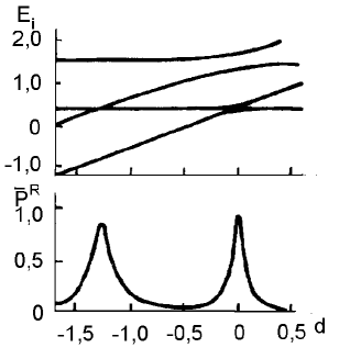
Figure 32: Dependence of subbarier energy levels $E_{i}$ for double asymmetric one-dimensional rectangular well with infinite external walls (a) and $\bar{p}^{R}$ , (b) from $d$ . Width of well is equal to $3$ , width of barrier - $1$ , height of barrier - $2$ .

Intuitively, we may suggest that $\bar{p}^{R}\approx 1$ if the initial minimum is local, and the final one is absolute. However, the results [58] obtained for the simplest one-dimensional models (asymmetric double wells of different shapes) are inconsistent with the intuitive expectations. The probability of tunneling from the local minimum to the absolute one resonantly depends on the potential parameters. Fig.32 gives the dependence of $\bar{p}^{R}$ from well depth displacement d. It is seen that at an arbitrary asymmetry $\bar{p}^{R}\ll 1$ .

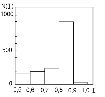
Figure 33: Distribution of subbarier wave functions $N\left(I\right)$ .

The resonant behaviour of $\bar{p}^{R}$ becomes clear if one considers the spatial structure of the subbarrier wave functions. For a sufficiently wide barrier at an arbitrary asymmetry, the subbarrier wave functions are largely localized in separate minima. Fig.33 gives the distribution $N\left(I\right)$ of the subbarrier wave functions as their degree of localization $I_{n}=\int\limits_{R}{\left|{\psi_{n}\left({\vec{r}}\right)}\right|^{2}d\vec{r}}$ for an accidental choice of the well depth displacement $d$. The delocalization takes place only in the vicinity of the quasicrossing of level. The degree of this delocalization is directly depends on the distance between the interacting levels. Obviously, the QWP, in which the components localized in the certain minimum are dominating, cannot effectively tunnel to the neighbouring minimum. This just explains the stringent correlation between the $\bar{p}^{R}$ minima and the level quasicrossing (see Fig. 32.)

Now the question arises if a similar correlation between the level quasicrossings, the delocalization of wave functions and resonant tunneling persists in the two-dimensional case. To give an answer to this question let us turn to the results of numerical investigation of stationary wave functions of Hamiltonian QON in region $W>16$ [59]. Recall that three ($C_{3v}$ - symmetry) identical additional minima appear at $W>16$ apart from the central minimum. The central minimum exceeds the lateral ones in depth in the region $16<W<18$. At $W>18$ , the central minimum becomes the local one. In this region of parameters the procedure of diagonalization of Hamiltonian QON in oscillator basis essentially complicates. It is connected with the fact, that the basis of Hamiltonian, the potential of which has the unique minimum, is used for the diagonalization of Hamiltonian possessing complex topology of the PES.

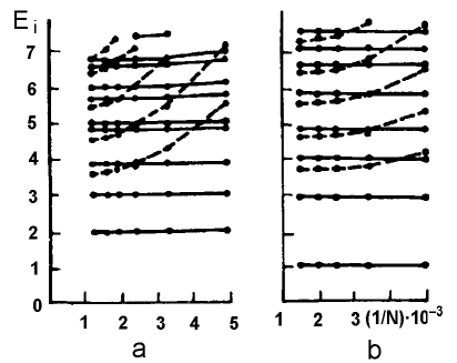
Figure 34: Dependence of energy spectrum $E$ -type (a) at $b=0.173798$ and $A_{1}$ -type (b) at $b=0.17$ from the dimension of submatrices $N$ for $W=17.8$ . Dashed lines correspond to the states localized in peripheral minima.

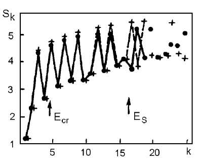
Figure 35: Dependence of $S_{k}$ from number of eigenstate $k$ ($A_{1}$ - type) for the dimension of submatrices 408 (dark point) and 690 (crosses) at $W=17.8$ and $b=0.17$ ; $E_{S}$ corresponds to saddle energy and $E_{cr}$ - the classical critical energy of the transition from regular type of motion to chaotic one.

In addition to large dimension of the basis it is necessary that the basis wave functions have sufficient value in the region of lateral minima. It is achieved by the optimization of oscillator frequency of basis $\omega_{0}$ . For the values of parameters used in the calculations $\left({W=17.8;b=0.17}\right)$ the value of oscillator frequency $\omega_{0}=0.2$ . Fig.34 gives low eigenvalues of $E$ and $A_{1}$ types depending on the basis dimension. We can see, that it is possible to get the saturation in basis at the dimension of submatrices $N\sim 10^{3}$ even for low states localized in the lateral minima (dashed lines).

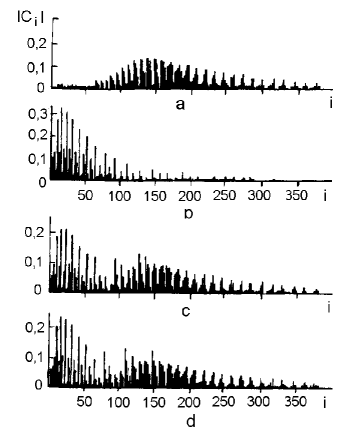
Figure 36: Distribution of coefficients $\left|{C_{i}}\right|$ by number of basis state $i=\{N,L,j\}$ ($E$ - type) for the localized states with $k=3$ (a) and $k=4$ (b) at $b=0.17379\;\left({W=17.8}\right)$ and for the delocalized states with $k=3$ (c) and $k=4$ (d) in the point of quasicrossing $b=0.1737924\;\left({W=17.8}\right)$ .

We can also use introduced above the analog of thermodynamic entropy $S_{k}$ for estimation of degree of saturation in basis. Fig.35 gives the $S_{k}$ values for the states of $A_{1}$ type for the dimension of submatrices 408 and 690. Increasing of the basis does not lead to sufficient changes of values $S_{k}$ for the states with energy up to saddle energy $E_{S}$ .

The states,localized in the central or in the lateral minima, have essentially different distributivity of coefficients $C_{i}^{k}\quad\left\{{i=NLj}\right\}$(see Fig. 36a,b) and thus different entropies: states, localized in the central minimum, have less entropy). In the neighbourhood of the points of level quasicrossings, the delocalization of wave functions, corresponding to these levels, takes place; these wave functions possess close distributivity of coefficients $C_{i}^{k}$ (see Fig. 36.c.d).

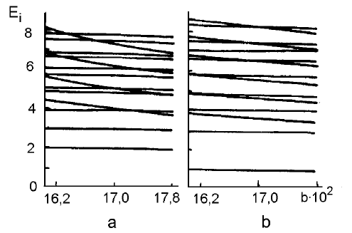
Figure 37: Dependence of energy levels $E_{i}$ of Hamiltonian (16.1) from the parameter $b$ for $W=17.8$ : a - spectrum of $E$ - type, b - spectrum of $A_{1}$ - type.

Fig.37 shows the subbarrier part of the energy spectrum obtained by the diagonalization. As it is easy to see the tunneling of the wave packet, composed of the subbarrier wave functions, can be described in the two-level approximation. Indeed, there are approximately 10 level quasicrossings of $A_{1}$ and $E$ - types, where the nonlinearity parameter changes are of the order of $10^{-2}$ . The effective half-width of the overlap integral in (64) is about $10^{-5}$ (see Fig. 38).Hence, all nondiagonal elements will be close to zero with the overwhelming probability in the matrix $\alpha_{mn}=\int\limits_{R}{\psi m^{*}\left({\vec{r}}\right)\psi_{n}}\left({\vec{r}}\right)d\vec{r}$ for an arbitrary nonlinearity parameter (e.g., $b$ ). Two appreciable different from zero nondiagonal matrix elements (two-level approximation) appear only in the vicinity of quasicrossings. The probability of double quasicrossings at a fixed nonlinearity parameter is almost excluded. This probability is by two or three orders lower than that of rather rare $\left({~{}10^{-3}}\right)$ single quasicrossings.

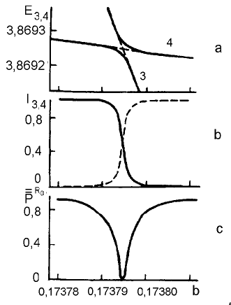
Figure 38: a - quasicrossing of energy levels of $E$ - type with $k=3,4$ for Hamiltonian (16.1); b - localization of wave functions of states with $k=3,4$ in the central well at different $b$ ; c - dependence $\bar{p}^{R}$ from $b$ .

So, now we can give the answer to the question we have posed above. The stringiest correlations between level quasicrossings, delocalization of wave functions and resonant tunneling across the potential barrier take place in the two-dimensional case (and, most likely, in the multi-dimensional one too).

The existence of the mixed state for the many-well potentials must be well manifested itself in dynamics of the QWP. Preexponential factor of the tunnel amplitude depends on the type of classical motion and consequently we expect to observe the asymmetry of the effective barrier penetration in the mixed. This purely classical effect may be observed only if the uncertainty in level energy is comparable with the average distance between levels and the system does not yet ”feels” that the spectrum is discrete. This determines the time scale for which observation of effect is possible. It is the same time scale on which transition from classical linear diffusive increasing of energy to quasiperiodical quantum evolution is observed [60].

2 Summary and open questions

2.1 Summary

In this review we have presented a complete description of classical dynamics generated by the Hamiltonian of quadrupole oscillations and identified those peculiarities of quantum dynamics which can be interpret as QMCS.

We have shown an intimate connection between dynamics features and geometry of the PES. Interpretation of negative curvature of the PES as the source of the local instability allowed to correctly predict the critical energy of the transition to chaos for one-well potentials.

Particular attention has been given to investigation of classical dynamics in the parameter region according to the PES with a few local minima. As is shown, one of the main peculiarities of the many-well Hamiltonians is the mixed state: at one at the same energy in a different local minima diverse dynamical regimes (regular or chaotic) are realized. Until the present time the most theoretical and numerical works have been focused on the behaviour of so-called billiards or Hamiltonian systems with the simplest topology of the PES. Evidently it is not enough for understanding of the real many-body systems with the complicated PES for which the mixed state is a situation of general position. Therefore the present review should be read as one of the indispensable steps on the way to transition from description of the model systems to direct consideration of much more realistic systems.

A new methodology for determination of the critical energy of the transition to chaos based on the investigation of correlations between dynamic features and geometry of the PES is developed for many-well potentials. It is more simpler than criteria of transition to chaos connected with one or other version of overlap resonance’s criterion. At the energies below the critical one approximate integrals of motion for every of local minima are derived by the Birkhoff-Gustavson normal form technique.

We have numerically demonstrated that for potential with a localized unstable region (in particular localized region of negative Gaussian curvature) regular motion restores at high energy, i.e. transition regularity-chaos-regularity takes place for these potentials.

QMCS in dynamics of QON have been the center of our consideration. The variations of statistical properties of energy spectrum in the process of $R-C-R$ transition have been studied in detail. For the chaotic region all the analyzed statistical characteristics are seen to be in good agreement with the GOE predictions. For regular regions our calculations are consistent with the hypothesis of the universal character of energy spectrum fluctuations. Though for small level spacings we observed some deviations which were probably due to a small admixture of the chaotic component.

We proved that the type of classical motion is correlated with the structure of the stationary wave functions of highly excited states in the $R-C-R$ transition. Correlations were found both in the coordinate space (the lattice of nodal curves and the distribution of the probability density) and in the Hilbert space associated with the integrable part of Hamiltonian (the distribution of the wave functions in the oscillator basis and the entropy of individual eigenstates). Calculations with the scaled Planck constant, which make it possible to obtain wave functions with equal quantum numbers and energies that correspond to different types of classical motion, enabled us to unambiguously isolate correlation effects in the structure of wave functions.

The Hamiltonian of QON was used as an example to study the shell structure destruction induced by the increase of nonintegrable perturbation term which models residual nucleon-nucleon interaction. In the vicinity of the classical critical energy value it was observed multiple formation of quasicrossings of the energy levels, violation of the quasiperiodical energy dependence of the entropy, and the increase of the average value fluctuations of the operators used to classify the eigenstate of the integrable problem.

The optimization of the basis frequency and, as a consequence, the possibility of diagonalization matrices of higher dimension made it possible to trace the restoration of the shell structure in the transition $C-R_{2}$ from chaos to regularity.

2.2 Open questions

The problem of studying of QMCS in Hamiltonian systems with a few local minima represents almost a noninvestigated region. We must take into account that, apart from conceptual difficulties, construction of spectrum and eigenfunctions in this case is a very difficult computational problem. Calculation of energy splitting $DE$ due to tunneling is one of the oldest problem of quantum mechanics. One dimensional problem for the most part is understood. A complication arises in the multidimensional problem, which might not have been expected until recently. This is because the semiclassical wave functions which determine energy splitting are sensitive to the nature of the classical motion. Wilkinson [104] calculated the energy splitting due to tunneling between a pair of quantum states which correspond to classical motion on tori in phase space. The case where both wave functions correspond to classical chaotic motion were discussed by Wilkinson and Hannay [105]. Problem of the wave function structure for the mixed state remains to be solved. The configuration space in this situation breaks up naturally into different regions (separate local minima), in each of which different dynamics regimes are realized. Thus, there is a need of a calculating scheme, which will enable us to use the partial information about each isolated region to obtain solution of the full problem. We believe that the path decomposition expansion of Auerbach and Kivelson [63] will prove to be useful for solving $2-d$ tunneling problem in the mixed state. This formalism allows to express the full time evolution operator as a time convolution and surface integrations of products of restricted Green functions, each of which involves the sum over paths that are limited to different regions of configuration space. Even for complicated nonseparable potential the qualitative behaviour is readily inferred and quantitative solutions can be obtained from knowledge of the classical dynamics.

In conclusion, we note that an important problem concerning the role of periodic orbit in the structure of wave functions was not considered in this study. In the semiclassical limit quantum state must be determined by the invariant sets formed by classical trajectories. These sets cover the total energy surface for systems that are chaotic in the classical limit. The approach in which the energy surface as a whole plays a dominant role is confirmed by the chaotic structure of nodal curves and by the random distribution of the probability density of the wave functions of highly exited states. However, the recent findings of Heller [64], who showed that wave functions can have the so-called scars corresponding to a high concentration of probability density near unstable periodic orbits, demonstrate that such an approach is not complete. The reason for this is that, although the measure of periodic trajectories is zero, their contribution is essentially singular, in contrast to the smooth contribution from the energy surface. These problems require special analysis for the Hamiltonian under study.

Acknowledgements The authors are grateful to A. Pashnev, G. Sotnikov and V. Yanovsky for fruitful discussions and valuable advices. The work was done with a partial support of the Basic Research Foundation of Ukraine (grant 383).

3 References