Magnetic moment and radius of the nucleon in a nonlocal model of meson-nucleon interaction

Abstract

Magnetic moment and radius of the nucleon are calculated in a nonlocal extension of the chiral linear $\sigma-$model. Properties of the nonlocal model under the vector and axial transformations are considered. The conserved electromagnetic and vector currents, and partially conserved axial vector current are obtained. In the calculation of the nucleon electromagnetic vertex the $\pi-$ and $\sigma-$loop diagrams are included. Contribution from vector mesons is added in the vector meson dominance model with a gauge-invariant photon-meson coupling. The nonlocality parameter associated with the $\pi N$ interaction is fixed from the experimental magnetic moment of the neutron. Other parameters (nonlocality parameter for the $\sigma N$ interaction and the mass of the $\sigma-$meson) are constrained by the magnetic moment of the proton. The calculated electric and magnetic mean-square radii of the proton and neutron are in satisfactory agreement with experiment.

I Introduction

Calculation of the nucleon magnetic moment has a long story. In fifties Fried [1] calculated pion-loop contribution to the electromagnetic (EM) form factors of the neutron. The authors of [2] pointed out to the importance of the Ward-Takahashi (WT) identity as a requirement for any model for the $\gamma NN$ vertex. Recoil corrections to the fixed-source static model [3] were calculated in [2] in a model with an extended pion-nucleon interaction and pseudo-vector (PV) coupling. However agreement between the theory and experimental values of the magnetic moments of the proton ($\mu_{p}$) and neutron ($\mu_{n}$) was poor.

The authors of [4, 5] evaluated the anomalous magnetic moments (AMM)s of the proton, $\kappa_{p}=\mu_{p}-1$, and the neutron, $\kappa_{n}=\mu_{n}$, while studying the $\gamma NN$ vertex of the off-mass-shell (bound) nucleon. Naus and Koch [4] calculated the off-shell EM form factors in the pion-loop approximation using the pseudo-scalar (PS) $\pi N$ interaction. The off-shell effects were shown to be appreciable, although the calculated AMMs, $\kappa_{p}=0.51,\,$ $\kappa_{n}=-3.7$, did not agree with the experimental values $\kappa_{p}^{\exp}\approx 1.793$ and $\kappa_{n}^{\exp}\approx-1.913$. A more refined approach based on the vector meson dominance (VMD) was applied in [5]. The pion-loop contribution and the $\pi NN$ form factors were included. To account for the gauge invariance of the $\gamma NN$ vertex the authors used a recipe from ref. [6]. It was shown [5] that the VMD vertex supplemented with the pion-loop contribution leads to a better description of AMMs, vis. $\kappa_{p}=1.9,$ $\kappa_{n}=-2.26$ for the PS, and $\kappa_{p}=1.74,$ $\kappa_{n}=-2.08$ for the PV $\pi N$ coupling. In a dynamical model [7] the effects of the $\Delta-$resonance and VMD were investigated in both the space-like and time-like regions of the photon momentum. An extended version of the VMD model was applied, which lead to results different from the conventional VMD model used in [5]. The calculated AMMs were $\kappa_{p}=1.45$ and $\kappa_{n}=-1.65$. Recently a non-perturbative approach for the $\gamma NN$ vertex has been developed in [8], where the infinite number of the pion loops was included. The magnetic form factor at the photon point was normalized to experiment.

In ref. [9] the chiral linear $\sigma-$model [10] has been applied in calculation of the AMM of the proton. Among other results it has been shown that the proton AMM can be reproduced with a heavy $\sigma-$meson ($m_{\sigma}\approx 800$ MeV). As follows from our calculation (sect. IV below) the neutron AMM turns out to be far off the experimental value. Thus it does not seem possible to describe simultaneously the proton and neutron AMMs in the linear $\sigma-$model, at least on the one-loop level.

In the present paper we develop a nonlocal extension of the linear $\sigma-$model, and apply it in calculation of the EM properties of the proton and neutron. We assume that the $\pi N$ ($\sigma N)$ interaction is governed by the form function $H_{\pi}(x^{\prime}-x,x^{\prime\prime}-x)$ ($H_{\sigma}(x^{\prime}-x,x^{\prime\prime}-x))$, where the space-time coordinates $x^{\prime},x^{\prime\prime}\$ stand for the nucleon, and $x$ for the meson. The nucleon mass is as usual generated through a non-zero vacuum expectation value of the $\sigma-$field, this leads to a constrained form function $H_{\sigma}(x^{\prime}-x,x^{\prime\prime}-x)=\delta^{4}(x^{\prime}-x^{\prime\prime})h_{\sigma}(x^{\prime}-x)$.  The similar form is used for the $\pi N$ function. The EM interaction in the model is included by making use of the minimal substitution in the so-called shift operators. This procedure generates, in addition to the nucleon and pion EM vertices, a sea-gull-like $NN\pi\gamma$ term. Properties of the nonlocal model under the $SU(2)$ axial and vector transformations are also different from properties of the local $\sigma-$model. We construct the conserved vector current and partially conserved axial current by applying the corresponding minimal substitutions in the action. These currents get contributions from the meson-nucleon interaction similarly to the EM current.

Further we calculate the $\gamma NN$ vertex in the covariant perturbation theory in the pion- and sigma-loop approximation. The cut-off in momentum space in the Fourier transforms of the functions $h_{\pi,\sigma}(x^{\prime}-x)$ ensures convergence of the loop integrals. Consistency of the calculation is verified by checking the WT identity. We concentrate on the magnetic moments and mean-square radii (MSR) of the proton and neutron and study contributions from various diagrams. For reasonable values of the nonlocality parameters and the $\sigma-$meson mass we find agreement between the calculation and experiment for AMMs. At the same time the $\pi-$ and $\sigma-$loop contributions turn out to be insufficient to describe the observed MSRs. For this reason the contributions coming from the vector mesons are added in the version [7] of the VMD model. In this version the photon couples to the vector mesons via a gauge-invariant Lagrangian. Inclusion of the $\rho-$ and $\omega-$mesons improves considerably description of the electric and magnetic MSRs of the proton and neutron.

The paper is organized as follows. In sect. II the nonlocal model is introduced. The conserved EM current is constructed. Properties of the model with respect to the axial and vector transformations are discussed and the corresponding currents are obtained. In sect. III the nucleon EM form factors are calculated in the one-loop approximation. Expressions for AMMs are derived. Lagrangian of the vector mesons is specified and their contributions to the EM form factors and MSRs are obtained. One important aspect of renormalization of the EM form factors is discussed. Results of the calculation of AMMs and MSRs, and discussion are presented in sect. IV. Conclusions are given in sect. V. Appendix A contains equations of motion in the nonlocal model. The Ward-Takahashi identity for the EM vertex is verified in Appendix B. Finally, Appendix C includes details of calculation of the loop integrals and expressions for the EM form factors, MSRs and the nucleon self-energy operator.

II Description of the model

Let us consider the following action for the nucleon ($N$), pion ($\vec{\pi}$), and sigma ($\phi$) fields

$$S=\int\{\bar{N}(x)i\partial/N(x)\,+\frac{1}{2}\,(\partial^{\mu}\vec{\pi}(x))^{2}+\frac{1}{2}(\partial^{\mu}\phi(x))^{2}-V(\phi,\vec{\pi})\}\mbox{\rm d}x+S_{int}\,,$$ (1)

$$S_{int}=-g\int\bar{N}(x^{\prime})[\phi(x)H_{\sigma}{(x^{\prime}-x,x^{\prime\prime}-x)}\, + i{\gamma_{5}\vec{\tau}\vec{\pi}(x)}H_{\pi}{(x^{\prime}-x,x^{\prime\prime}-x)]}$$ (3)

$$\quad\quad\quad\quad\quad\quad\quad\quad\times N(x^{\prime\prime})\ \mbox{\rm d}x\mbox{\rm d}x^{\prime}\mbox{\rm d}x^{\prime\prime}\,,$$

where $g$ is the coupling constant, $\mbox{\rm d}x=\mbox{\rm d}^{4}x,$ $\partial^{\mu}=\partial/\partial x_{\mu}$ ,  ${\partial/=\gamma}_{\mu}\partial^{\mu}$ and

$$V(\phi,\vec{\pi})=\frac{\lambda}{4}[\phi(x)^{2}+{{{\vec{\pi}}(x)}}^{2}-\xi^{2}]^{2}-c\phi(x)\,$$ (4)

is the meson potential. Eq. (3) is a nonlocal extension of the meson-nucleon interaction in the chiral $SU(2)_{L}\times SU(2)_{R}$ linear $\sigma-$model with explicit symmetry-breaking term  $c\phi$ (see, e.g., [11], Ch.11, sect.11.4.1, or [12], Ch.5, sect.2.6). The three-point form functions $H_{\pi,\sigma}(x^{\prime}-x,x^{\prime\prime}-x)$ due to the translational invariance depend on the two four-vectors. After imposing the Lorentz invariance they become functions of $s_{1}=(x^{\prime}-x)^{2}$, $s_{2}=(x^{\prime\prime}-x)^{2}$ and $s_{12}=(x^{\prime}-x^{\prime\prime})^{2}$. In general, $H_{\pi,\sigma}(x^{\prime}-x,x^{\prime\prime}-x)$ should fall off at $|s_{1}|$, $|s_{2}|,$ $|s_{12}|\ \rightarrow\ \infty$ and have correct local limit. At this point we refer to [13, 14] where different aspects of the nonlocal $\bar{\psi}\psi\phi$ model [15] for the nucleon and neutral meson fields were considered. A review of some nonlocal theories can be found in monographs [16].

In the same way as in the local model we take $\phi(x)=\langle\phi\rangle+\sigma(x)$ and require the minimum of $V(\langle\phi\rangle,\langle\vec{\pi}\rangle)$ to be at $\langle\phi\rangle=f_{\pi}$ and $\langle\vec{\pi}\rangle=0,$ where $f_{\pi}$ is the $\pi^{+}\rightarrow\mu^{+}\nu_{\mu}$  weak-decay constant. This gives  $\xi^{2}=f_{\pi}^{2}-{c}/\lambda f_{\pi}$  and the action takes the form

$$S=\int\{\bar{N}(x)(i\partial/-m_{N})N(x)\,+\frac{1}{2}[(\partial^{\mu}\vec{\pi}(x))^{2}-m_{\pi}^{2}] + \frac{1}{2}[(\partial^{\mu}\sigma(x))^{2}-m_{\sigma}^{2}]$$ (6)

$$-V^{\prime}(\sigma{,\vec{\pi})}\}\ \mbox{\rm d}x+S_{int}^{\prime}\,,$$

$$V^{\prime}(\sigma,\vec{\pi})=\lambda[\sigma(x)^{2}+\vec{\pi}(x)^{2}]\{f_{\pi}\sigma(x)+\frac{1}{4}[\sigma(x)^{2}+\vec{\pi}(x)^{2}]\}+\mbox{\rm const}\,,$$ (7)

and $S_{int}^{\prime}$ is obtained from $S_{int}$ in eq. (3) after replacing $\phi(x)$ by $\sigma(x)$. The masses of the pion, sigma and nucleon are defined respectively by

$$m_{\pi}^{2}=\frac{c}{f_{\pi}},\;\ \ \ \ \ \ \ \ \ \ \ \ \ \ \ m_{\sigma}^{2}=2\lambda f_{\pi}^{2}+\frac{c}{f_{\pi}}\,,\;\ \ \ \ \ \ \;\;\ \ \ \ \ \ \ \ m_{N}=gf_{\pi}\ F_{\sigma}$$ (8)

with a constant $F_{\sigma}.$ In order to reproduce the nucleon mass term the following condition

$$gf_{\pi}\int{\bar{N}(x^{\prime})N(x^{\prime\prime})H_{\sigma}{(x^{\prime}-x,x^{\prime\prime}-x)}\,\mbox{\rm d}x\mbox{\rm d}x^{\prime}\mbox{\rm d}x^{\prime\prime}}=m_{N}\int\bar{N}(x)N(x)\mbox{\rm d}x$$ (9)

has been imposed. From eq. (9) one obtains the constraint

$$\int H{{}_{\sigma}\ {(x^{\prime}-x,x^{\prime\prime}-x)}\,\mbox{\rm d}x=\delta^{4}(x}^{\prime}-x^{\prime\prime})F_{\sigma}\,.$$ (10)

We further introduce the Fourier transforms

$$\hat{H}_{\pi,\sigma}(p^{\prime},p^{\prime\prime})=\int{\exp}[{{-i(p^{\prime}\cdot y}}^{\prime}{-p}^{\prime\prime}{\cdot y}^{\prime\prime}{{)]}\ }{H}{{}_{\pi,\sigma}(y^{\prime},y}^{\prime\prime}{)\ \mbox{\rm d}y}^{\prime}{\mbox{\rm d}y}^{\prime\prime}\,,$$ (11)

with notation $a\cdot b\equiv a_{\nu}b^{\nu}$. Then eqs. (10) and (11) lead to the constraint in the momentum space $\hat{H}_{\sigma}(p,p)=F_{\sigma}$ for any $p$. Hence $\hat{H}_{\sigma}(p^{\prime},p^{\prime\prime})$ should depend on $p^{\prime}-p^{\prime\prime}$, or $\hat{H}_{\sigma}(p^{\prime},p^{\prime\prime})=\hat{h}_{\sigma}(p^{\prime}-p^{\prime\prime}).$ We will also choose  $\hat{H}_{\pi}(p^{\prime},p^{\prime\prime})=\hat{h}_{\pi}(p^{\prime}-p^{\prime\prime})$ for the pion-nucleon interaction. In configuration space one has $H_{\pi,\sigma}(x^{\prime}-x,x^{\prime\prime}-x)=\delta^{4}(x^{\prime}-x^{\prime\prime})h_{\pi,\sigma}(x^{\prime}-x)$, where

$${h}_{\pi,\sigma}(y)=(2\pi)^{-4}\int{\exp}(ik\cdot y)\hat{h}_{\pi,\sigma}(k)\ \mbox{\rm d}^{4}k\,$$ (12)

with $\hat{h}_{\sigma}(0)=F_{\sigma}$ due to eq. (10). The normalization of the form factors $\hat{h}_{\pi,\sigma}(k)$ at $k=0$ is specified in subsect. III A. The constrained form function $h_{\pi}(x^{\prime}-x)$ or $h_{\sigma}(x^{\prime}-x)$ describes an extended interaction between the meson and the nucleon source, whereas due to $\delta^{4}(x^{\prime}-x^{\prime\prime})$ there is no internal coupling of the nucleon to itself.

The interaction (3) can be rewritten for convenience as follows

$$S_{int} = -g\int[\phi{{(x)}\,}\tilde{\rho}_{S}{(x)+}\vec{\pi}{(x)}\tilde{\vec{\rho}}{{}_{A}{(x)]\mbox{\rm d}x}\,,}$$ (13)

$$\tilde{\rho}_{S}(x) = \int\rho_{S}{(x}^{\prime}{)h}_{\sigma}(x^{\prime}-x)\mbox{\rm d}x^{\prime}\,,\,\ \ \ \ \ \ \ \rho_{S}(x^{\prime})={\bar{N}(x^{\prime})N(x^{\prime})}\,,$$ (14)

$$\tilde{\vec{\rho}}_{A}(x) = \int\vec{\rho}_{A}{(x}^{\prime}{)h}_{\pi}(x^{\prime}-x)\mbox{\rm d}x^{\prime}\,,\,\;\ \ \ \ \ \vec{\rho}_{A}(x^{\prime})=\bar{N}(x^{\prime})i\gamma_{5}\vec{\tau}N(x^{\prime})\,.$$ (15)

A Electromagnetic current

In this subsection we discuss properties of the model under the gauge $U(1)$ transformation. Note first that variation of the action (1) with $S_{int}$ in eq. (13) under arbitrary infinitesimal variation of the fields leads to

$$\delta S=\int\frac{\partial}{\partial x^{\mu}}[\bar{N}(x)i\gamma^{\mu}\delta N(x)+\partial^{\mu}\phi(x)\delta\phi(x)+\partial^{\mu}\vec{\pi}(x)\delta\vec{\pi}(x)]\mbox{\rm d}x\,,$$ (16)

where equations of motion have been used (see Appendix A). Let us take the transformation

$$N \rightarrow N-i\epsilon\ e\hat{Q}_{p}N\,,\;\ \ \ \ \ \ \ \ \bar{N}\rightarrow\bar{N}+i\epsilon\ \bar{N}e\hat{Q}_{p}\,,$$ (17)

$$\vec{\pi} \rightarrow \vec{\pi}-i\epsilon\ e\hat{Q}_{\pi}\vec{\pi}\,,\;\ \ \ \ \ \ \ \ \ \ \phi\rightarrow\phi$$ (18)

with the parameter $\epsilon.\$ In eqs. (18) $e$ is the proton charge, $\hat{Q}_{p}={\frac{1}{2}}(1+\tau_{3})$ and $\hat{Q}_{\pi}=t_{3}$, where ${\vec{\tau}}$  and $\vec{t}$ are the isospin matrices for the nucleon and the pion respectively. For the constant $\epsilon$ the action is clearly invariant, i.e. $\delta S=0$, and therefore the following integral analogue of the current conservation holds

$$\int\frac{\partial}{\partial x^{\mu}}[{J}_{N,em}^{\mu}(x)+J_{\pi,em}^{\mu}(x)]\mbox{\rm d}x=0\,,$$ (19)

where the nucleon and the pion EM currents are defined as $J_{N,em}^{\mu}(x)=e\bar{N}(x)\gamma^{\mu}\hat{Q}_{p}N(x)$ and $J_{\pi,em}^{\mu}(x)=-ie\partial^{\mu}\vec{\pi}\hat{Q}_{\pi}\vec{\pi}=e(\vec{\pi}\times\partial^{\mu}\vec{\pi})_{3}$. Eq. (19) is in line with ref. [18] where integral conservation laws were studied for a general nonlocal action, and with ref. [13] where the related issues were addressed, in particular construction of the baryon charge and four-vector of the energy-momentum in framework of the nonlocal model [15].

Despite eq. (19) the current ${J}_{N,em}^{\mu}(x)+J_{\pi,em}^{\mu}(x)$ is not locally conserved, i.e.,  $\partial_{\mu}[{J}_{N,em}^{\mu}(x)+J_{\pi,em}^{\mu}(x)]\neq 0.$ A conserved current can be constructed by making use of the minimal substitution

$$\partial_{x}^{\mu}\rightarrow\partial_{x}^{\mu}+ie\hat{Q}A^{\mu}(x)\,,$$ (20)

where $A^{\mu}(x)\,$ is the EM field, $\partial_{x}^{\mu}=\partial/\partial x_{\mu}$ and $\hat{Q}=\hat{Q}_{p}$ or $\hat{Q}_{\pi}.$ The free nucleon and meson terms in the action (1) give rise to the currents  $J_{N,em}^{\mu}(x)$ and  $J_{\pi,em}^{\mu}(x).$ In order to apply eq. (20) to the interaction (13) we represent the $\pi N$ piece of  $S_{int}$ in the form

$$S_{\pi N} = -g\int\int\vec{\pi}(x)\vec{\rho}_{A}(x+y)h_{\pi}(y)\ \mbox{\rm d}x\mbox{\rm d}y$$ (21)

$$= -g\int\int\vec{\pi}(x)[\exp(y\cdot\partial_{x})N(x)]^{\dagger}\gamma_{0}i\gamma_{5}\vec{\tau}[\exp(y\cdot\partial_{x})N(x)]h_{\pi}(y)\ \mbox{\rm d}x\mbox{\rm d}y\,,$$ (22)

where the ‘shift’ operator $\ {\exp(y\cdot\partial_{x})}$ acts on the nucleon field as follows: $\exp(y\cdot\partial_{x})N(x)=N(x+y)$. After substituting eq. (20) in eq. (22) one can use the identity

$$\exp(O_{1}+O_{2}) = \bar{{\cal P}}\exp[\,\int_{0}^{1}O_{2}(t)\,\mbox{\rm d}t\,]\,\exp(O_{1})\,,$$ (23)

$$O_{2}(t) = \exp(O_{1}t)O_{2}\exp(-O_{1}t)\,,$$ (24)

for any operators $O_{1}$ and $O_{2}$, where $\bar{{\cal P}}\exp[...]$ denotes the exponential antiordered in the parameter $t$. Choosing $O_{1}=y\cdot{\partial_{x}}$ and $\ O_{2}=ie\hat{Q}_{p}y\cdot A(x)$ one obtains

$$S_{\pi N}\rightarrow S_{\pi N}\{A\} = -g\int\int\vec{\pi}(x)\bar{N}(x^{\prime})\,{\cal P}\exp[-ie\chi(x^{\prime},x)]\,i\gamma_{5}\vec{\tau}$$ (26)

$$\times\bar{{\cal P}}\exp[ie\chi(x^{\prime},x)]N(x^{\prime})\ {h_{\pi}{(x^{\prime}-x)}}\ \mbox{\rm d}x\mbox{\rm d}x^{\prime}\,,$$

$$\chi(x^{\prime},x) = (x^{\prime}-x)\cdot\int_{0}^{1}\hat{Q}_{p}{A(x(1-t)+x}^{\prime}{t)\,\mbox{\rm d}t}\,$$ (27)

with ${\cal P}\exp[...]$ being the ordered in $t$ exponential. The modified interaction $S_{\pi N}\{A\}$ is invariant under the transformations (18) with the $x-$dependent parameter $\epsilon(x)$, if the EM field transforms as $A^{\mu}(x)\rightarrow A^{\mu}(x)+\partial^{\mu}\epsilon(x)$. The $\sigma N$ term does not give rise to the EM interaction.

We should note that eq. (26) gives the EM interaction in all orders in charge. In the first order in $e$ we obtain the current by taking the functional derivative

$$J_{\pi N,em}^{\mu}(x)=-\frac{\delta}{\delta A_{\mu}(x)}S_{\pi N}\{A\}|_{A=0}$$ (28)

$$=-eg\int\int[\vec{\rho}_{A}(y)\times\vec{{\pi}}(z)]_{3}\ (y-z)^{\mu}\int_{0}^{1}\delta^{4}{(x-z(1-t)-y}t)\,\mbox{\rm d}t\ h_{\pi}(y-z)\ \mbox{\rm d}y\mbox{\rm d}z\,.$$ (29)

Now direct calculation shows that the total EM current is conserved, i.e.,

$$\frac{\partial}{\partial x^{\mu}}[{J}_{N,em}^{\mu}(x)+J_{\pi,em}^{\mu}(x)+J_{\pi N,em}^{\mu}(x)]=0\,.$$ (30)

In case of the local $\pi N$ interaction, $\ h_{\pi}(y-z)\rightarrow\delta^{4}(y-z)$, the current $J_{\pi N,em}^{\mu}(x)$ vanishes.

One should keep in mind that there is an ambiguity in construction of the current $J_{\pi N,em}^{\mu}(x).$ Additional gauge invariant terms appear if the integral in eq. (26) along the straight line

$$\int_{0}^{1}(x^{\prime}-x)\cdot{A(x(1-t)+}x^{\prime}t{)\,\mbox{\rm d}t}=\int_{x}^{x^{\prime}}{A}^{\mu}\,{\mbox{\rm d}l}_{\mu}$$ (31)

is replaced by the integral over an arbitrary contour connecting the points $x^{\nu}$ and $x^{\prime\nu}.$ This was noticed long ago by Bloch [19] when developing a nonlocal theory. Our following consideration is restricted to the straight-line integration.

Finally note that the minimal substitution in the shift operator was applied earlier in [20, 21]. In particular, in [21] the EM current for the two nucleons in the Bethe-Salpeter formalism was constructed; there also some additional gauge-invariant contributions, proportional to the EM tensor $F^{\mu\nu}(x),$ were discussed.

B Axial and vector currents

Properties of the model under the isospin transformation with the parameters $\epsilon^{a}\;\;(a=1,2,3)$

$$N \rightarrow N-i\frac{\vec{\tau}}{2}\vec{\epsilon}\ N\,,\;\ \ \ \ \ \ \ \ \ \ \bar{N}\rightarrow\bar{N}+\bar{N}\ i\frac{\vec{\tau}}{2}\vec{\epsilon}\,,$$ (32)

$$\ \vec{\pi} \rightarrow \vec{\pi}+\vec{\epsilon}\times\vec{\pi}\,,\;\ \ \ \ \ \ \ \ \ \ \ \ \ \phi\rightarrow\phi\,.$$ (33)

are similar to the case considered in the previous subsection. It is easy to show from eq. (16) that the integral conservation law

$$\int\frac{\partial}{\partial x^{\mu}}[\vec{J}_{N,vec}^{\mu}(x)+\vec{J}_{\pi,vec}^{\mu}(x)]\mbox{\rm d}x=0$$ (34)

is fulfilled, where $\vec{J}_{N,vec}^{\mu}(x)=\bar{N}(x)\gamma^{\mu}\frac{\vec{\tau}}{2}N(x)$ and $\ \vec{J}_{\pi,vec}^{\mu}(x)=\vec{\pi}(x)\times\partial^{\mu}\vec{\pi}(x)$ are the conventional nucleon and pion vector currents.

The axial $SU(2)$ transformation in the nonlocal $\sigma-$model is a more interesting case because the action is not invariant under the transformation. Consider the following variation of the fields

$$N \rightarrow N-i\gamma_{5}\frac{\vec{\tau}}{2}\vec{\epsilon}\ N\,,\;\ \ \ \ \ \ \bar{N}\rightarrow\bar{N}-\bar{N}\ i\gamma_{5}\frac{\vec{\tau}}{2}\vec{\epsilon}\,,$$ (35)

$$\ \vec{\pi} \rightarrow \vec{\pi}+\vec{\epsilon}\phi\,,\;\ \ \ \ \ \ \ \ \ \ \ \ \ \ \ \phi\rightarrow\phi-\vec{\epsilon}\vec{\pi}\,.$$ (36)

For the constant parameters $\epsilon^{a}$ it follows from eq. (16) that

$$\delta S=\vec{\epsilon}\int\frac{\partial}{\partial x^{\mu}}[\vec{J}_{N,ax}^{\mu}(x)+\vec{J}_{M,ax}^{\mu}(x)]\mbox{\rm d}x\,,$$ (37)

where the nucleon and the meson axial currents are $\vec{J}_{N,ax}^{\mu}(x)=\bar{N}(x)\gamma^{\mu}\gamma_{5}\frac{\vec{\tau}}{2}N(x)$ and $\vec{J}_{M,ax}^{\mu}(x)=\partial^{\mu}\vec{\pi}(x)\phi(x)-\partial^{\mu}\phi(x)\vec{\pi}(x)$ respectively. The same variation $\delta S$ can be calculated directly by making use of $\ \delta\rho_{S}(x)=-\vec{\epsilon}\vec{\rho}_{A}(x)\$ and $\ \delta\vec{\rho}_{A}(x)=\vec{\epsilon}\rho_{S}(x).\$ Then comparison of the result with eq. (37) yields the equation

$$\int\frac{\partial}{\partial x^{\mu}}[\vec{J}_{N,ax}^{\mu}(x)+\vec{J}_{M,ax}^{\mu}(x)]\mbox{\rm d}x=-c\int\vec{\pi}(x)\mbox{\rm d}x$$ (38)

$$\;\ \ \ \ \ \ \ \ \ \ \ \ \ \ \ \ \ \ \ \ +g\int\int[\rho_{S}{(x}^{\prime}{)\vec{\pi}(x)+\vec{\rho}}_{A}(x^{\prime})\phi(x)][{h}_{\sigma}(x^{\prime}-x)-{h}_{\pi}(x^{\prime}-x)]\mbox{\rm d}x\mbox{\rm d}x^{\prime}\,.$$ (39)

The first term on the r.h.s. of eq. (39) comes from the symmetry-breaking term $c\phi$ leading to the finite pion mass, while the second term is related to the difference between the form functions for the $\sigma N$ and $\pi N$ interactions.

Note that eqs. (34) and (39) are the integral relations from which the corresponding local relations do not follow. In order to find the axial and vector currents satisfying the local relations let us use the following ‘minimal’ substitutions

$$\partial^{\mu}N(x) \rightarrow \{\partial^{\mu}+i\frac{\vec{\tau}}{2}[\gamma_{5}\vec{a}^{\mu}(x)+\vec{\rho}^{\mu}(x)]\}N(x)\,,$$ (40)

$$\partial^{\mu}\vec{\pi}(x) \rightarrow \partial^{\mu}\vec{\pi}(x)-\phi(x)\vec{a}^{\mu}(x)+\vec{\pi}(x)\times\vec{\rho}^{\mu}(x)\,,$$ (41)

$$\partial^{\mu}\phi(x) \rightarrow \partial^{\mu}\phi(x)+\vec{\pi}(x)\vec{a}^{\mu}(x)\,,$$ (42)

where the axial vector field $\vec{a}^{\mu}(x)$ and the vector field $\vec{\rho}^{\mu}(x)$ are introduced. They transform according to ([12], Ch.5, sect.4.3)

$$\vec{\rho}^{\mu}\rightarrow\vec{\rho}^{\mu}+\vec{\epsilon}\times\vec{\rho}^{\mu}+\partial^{\mu}\vec{\epsilon}\,,\;\;\;\;\;\;\;\;\;\;\;\;\;\;\vec{a}^{\mu}\rightarrow\vec{a}^{\mu}+\vec{\epsilon}\times\vec{a}^{\mu}$$ (43)

under the isospin rotations, and

$$\vec{\rho}^{\mu}\rightarrow\vec{\rho}^{\mu}+\vec{\epsilon}\times\vec{a}^{\mu}\,,\;\;\;\;\;\;\;\;\;\;\;\;\;\;\vec{a}^{\mu}\rightarrow\vec{a}^{\mu}+\vec{\epsilon}\times\vec{\rho}^{\mu}+\partial^{\mu}\vec{\epsilon}$$ (44)

under the chiral rotations described by the $x-$dependent parameters $\epsilon^{a}(x)$. The axial and vector currents can be obtained by taking the functional derivatives

$$\vec{J}_{ax}^{\mu}(x)=-\frac{\delta}{\delta\vec{a}_{\mu}(x)}S\{a,\rho\}|_{a=\rho=0}\,,\;\ \ \ \ \ \ \ \ \vec{J}_{vec}^{\mu}(x)=-\frac{\delta}{\delta\vec{\rho}_{\mu}(x)}S\{a,\rho\}|_{a=\rho=0}\,.$$ (45)

Applying eqs. (42) to the free nucleon and meson terms in the action gives the axial current $\vec{J}_{N,ax}^{\mu}(x)+\vec{J}_{M,ax}^{\mu}(x)$ and the vector current $\vec{J}_{N,vec}^{\mu}(x)+\vec{J}_{\pi,vec}^{\mu}(x)$ defined above after eqs. (37) and (34). Those coincide with the currents in the local $\sigma-$model ([11], Ch.11, sect.11.4.1). Additional contributions arise from the nonlocal interaction. Proceeding similarly to the derivation of the EM interaction in subsect. II A we obtain

$$S_{int}\rightarrow S_{int}\{a,\rho\}= - g\int\int{\bar{N}(x}^{\prime}{)}{{\cal P}}\exp[-i{\varphi}(x^{\prime},x)+i\gamma_{5}{\psi}(x^{\prime},x)]\{\phi(x){{h_{\sigma}{(x}}}^{\prime}-x{)}$$ (46)

$$+ i\gamma_{5}\vec{\tau}\vec{\pi}(x){{h_{\pi}{(x}}}^{\prime}-x{)\}}\bar{{\cal P}}\exp[i{\varphi}(x^{\prime},x)+i\gamma_{5}{\psi}(x^{\prime},x)]N(x^{\prime})\ \mbox{\rm d}x\mbox{\rm d}x^{\prime}\,,$$ (47)

$${\varphi}(x^{\prime},x) = \frac{1}{2}(x^{\prime}-x)\cdot\int_{0}^{1}\vec{\tau}{\vec{\rho}{(x(1-t)+x}^{\prime}{t)}\,\mbox{\rm d}t}\,,\;\ \ \ \ \ \ \ \$$ (48)

$${\psi}(x^{\prime},x) = \frac{1}{2}(x^{\prime}-x)\cdot\int_{0}^{1}\vec{\tau}\vec{a}{(x(1-t)+x}^{\prime}{t)\,\mbox{\rm d}t\,.}$$ (49)

It is straightforward now to obtain the currents from eqs. (45) and (47). The axial vector current is

$$\vec{J}_{MN,ax}^{\mu}(x) = -g\int\int[\rho_{S}(y)\vec{\pi}(z)h_{\pi}(y-z)-\vec{\rho}_{A}(y)\phi(z)h_{\sigma}(y-z)](y-z)^{\mu}$$ (51)

$$\times\int_{0}^{1}\delta^{4}{(x-z(1-t)-y}t)\,\mbox{\rm d}t\ \mbox{\rm d}y\mbox{\rm d}z\,,$$

and the vector current is

$$\vec{J}_{\pi N,vec}^{\mu}(x)=-g\int\int[\vec{\rho}_{A}(y)\times\vec{\pi}(z)]\ (y-z)^{\mu}\int_{0}^{1}\delta^{4}{(x-z(1-t)-y}t)\,\mbox{\rm d}t\ h_{\pi}(y-z)\ \mbox{\rm d}y\mbox{\rm d}z\,.$$ (52)

One can also show that

$$\int\frac{\partial}{\partial x^{\mu}}\vec{J}_{MN,ax}^{\mu}(x)\mbox{\rm d}x=\int\frac{\partial}{\partial x^{\mu}}\vec{J}_{\pi N,vec}^{\mu}(x)\mbox{\rm d}x=0\,,$$ (53)

though the divergences of the currents do not vanish. Eqs. (51) and (52) are sufficient to obtain the locally conserved vector current and partially conserved axial current that obey equations

$$\frac{\partial}{\partial x^{\mu}}[\vec{J}_{N,vec}^{\mu}(x)+\vec{J}_{\pi,vec}^{\mu}(x)+\vec{J}_{\pi N,vec}^{\mu}(x)] = 0\,,$$ (54)

$$\frac{\partial}{\partial x^{\mu}}[\vec{J}_{N,ax}^{\mu}(x)+\vec{J}_{M,ax}^{\mu}(x)+\vec{J}_{MN,ax}^{\mu}(x)] = -c\vec{\pi}(x)+g\int[\rho_{S}(x^{\prime})\vec{\pi}(x)$$ (56)

$$+\vec{\rho}_{A}(x^{\prime})\phi(x)][h_{\sigma}(x^{\prime}-x)-h_{\pi}(x^{\prime}-x)]\mbox{\rm d}x^{\prime}\,,$$

where we can substitute $\phi(x)=f_{\pi}+\sigma(x)\$ and $c=f_{\pi}m_{\pi}^{2}.$ If the form functions for the pion and sigma are equal to each other then the axial current satisfies the simpler equation

$$\frac{\partial}{\partial x^{\mu}}[\vec{J}_{N,ax}^{\mu}(x)+\vec{J}_{M,ax}^{\mu}(x)+\vec{J}_{MN,ax}^{\mu}(x)]=-c\vec{\pi}(x)\,.$$ (57)

Apparently the currents (51) and (52) vanish for the local $\pi N$ and $\sigma N$ interactions, i.e., if $h_{\pi}(y-z)\rightarrow\delta^{4}(y-z)$, $\ h_{\sigma}(y-z)\rightarrow\delta^{4}(y-z)$. In this case all equations of the local $\sigma-$model are restored.

In general case, taking the matrix element of eq. (56) at $x^{\mu}=0$ between the one-pion state and the vacuum leads, in the lowest order, to the PCAC relation

$$\langle 0|\partial_{x}\cdot[{J}_{N,ax}^{a}(0)+{J}_{M,ax}^{a}(0)+{J}_{MN,ax}^{a}(0)]|\pi^{b}(\vec{q})\rangle$$ (58)

$$=-c\delta^{ab}+g[\hat{h}_{\sigma}{(0)-}\hat{h}_{\pi}{(0)}]\ \langle 0|\rho_{S}(0)|0\rangle\delta^{ab}=-f_{\pi}m_{\pi}^{2}\delta^{ab}\,,$$ (59)

where the pion states are normalized as follows: $\langle\pi^{a}(\vec{q}^{\prime})|\pi^{b}(\vec{q})\rangle=(2\pi)^{3}2\omega_{q}\delta^{3}(\vec{q}-\vec{q}^{\prime})\delta^{ab}$  with $\omega_{q}^{2}=\vec{q}^{2}+m_{\pi}^{2}$, and $a,b=1,2,3$.  The term in eq. (59) proportional to $g$ does not contribute because it involves the nucleon operators. The zero vacuum expectation value of $\rho_{S}(0)$ can be ensured by choosing the normal ordering of the nucleon operators in $S_{int}$. Besides, one can normalize the form factors so that $\hat{h}_{\pi}(0)=\hat{h}_{\sigma}(0)$. It is seen that on the level of the matrix element the PCAC relation has the same form as in the local $\sigma-$model [10]. On the operator level however there is an additional term in eq. (56) proportional to the difference between the nonlocality functions for the $\pi-$ and $\sigma-$ mesons.

The axial properties of the nucleon will be addressed in detail elsewhere. Now we proceed to the calculation of the nucleon EM vertex.

III Magnetic moment and mean-square radius of the nucleon

A Pion- and sigma-loop contributions to the electromagnetic vertex

To calculate the nucleon EM vertex we start with the 3-point Green function

$$G_{\nu}(x_{2},x_{1};z)=\langle 0|TN(x_{2})\bar{N}(x_{1})A_{\nu}(z)|0\rangle$$ (60)

$$= (2\pi)^{-8}\int{\exp[i(p_{2}x_{2}-p_{1}x_{1}-qz)]\delta^{4}(p_{1}+q-p_{2})G_{\nu}(p_{2},p_{1};q)\ \mbox{\rm d}^{4}p_{1}\mbox{\rm d}^{4}p_{2}\mbox{\rm d}^{4}q}\,,$$ (61)

where $T$ is the time-ordering operator. The Fourier transform $G_{\nu}(p_{2},p_{1};q)$ of the Green function is related to the irreducible $\gamma NN$ vertex function $\Gamma^{\mu}(p_{2},p_{1};q)$ via

$$G_{\nu}(p_{2},p_{1};q)=iS^{\prime}(p_{2})[-ie\Gamma^{\mu}(p_{2},p_{1};q)]iS^{\prime}(p_{1})[-iD_{\mu\nu}^{\prime}(q)]\,,$$ (62)

where $S^{\prime}(p)$ ($D_{\mu\nu}^{\prime}(q)$) is the nucleon (photon) dressed propagator, and $p_{2}=p_{1}+q$. Next step is evaluation of the lowest order contributions to $\Gamma^{\mu}(p_{2},p_{1};q)$ in the perturbation theory. We take into account the pion- and sigma-loop diagrams (see fig. 1 ‘a,b,c’ and ‘d$\pm$’) which include contributions of the order $g^{2}.$ The proton and neutron vertex functions read

$$\Gamma^{\mu}_{p}(p_{2},p_{1};q)=\gamma^{\mu}-\Gamma_{a}^{\mu}+{\frac{1}{2}}\Gamma_{b}^{\mu}+\Gamma_{c}^{\mu}+\Gamma_{d+}^{\mu}\,,$$ (63)

$$\Gamma^{\mu}_{n}(p_{2},p_{1};q)=\Gamma_{a}^{\mu}+\Gamma_{b}^{\mu}+\Gamma_{d-}^{\mu}\,,$$ (64)

where $\Gamma_{a}^{\mu}$ is the $\pi-$loop term with the photon coupled to the pion, $\Gamma_{b}^{\mu}$ ($\Gamma_{c}^{\mu}$) is the $\pi-$loop ($\sigma-$loop) term with the photon attached to the proton:

$$\Gamma_{a}^{\mu} = C\int{\Delta}_{\pi}{(k)\Delta_{\pi}}{(k-q)(2k-q)^{\mu}\hat{h}}_{\pi}{(k)\gamma}_{5}{S(p_{2}-k){\gamma}_{5}\hat{h}_{\pi}}{(q-k)\ \mbox{\rm d}^{4}k}\,,$$ (65)

$$\Gamma_{b}^{\mu} = -C\int{\Delta}_{\pi}{(k)\hat{h}_{\pi}}{(k){\gamma}_{5}S(p_{2}-k)\gamma^{\mu}S(p_{1}-k){\gamma}_{5}\hat{h}_{\pi}}{(-k)\ \mbox{\rm d}^{4}k}\,,$$ (66)

$$\Gamma_{c}^{\mu} = \frac{1}{2}C\int{\Delta}_{\sigma}{(k)\hat{h}_{\sigma}}{(k)S(p_{2}-k)\gamma^{\mu}S(p_{1}-k)\hat{h}_{\sigma}}{(-k)\ \mbox{\rm d}^{4}k}\,,$$ (67)

$\Delta_{\pi,\sigma}(k)=(k^{2}-m_{\pi,\sigma}^{2}+i0)^{-1}$ ($S(p)=({p/}-m_{N}+i0)^{-1}$) is the free meson (nucleon) propagator with physical value of the meson (nucleon) mass, and $C\equiv 2ig^{2}(2\pi)^{-4}$. The contributions coming from $J_{\pi N,em}^{\mu}$ in eq. (29) are

$$\Gamma_{d+}^{\mu}=-\Gamma_{d-}^{\mu} = C\int\Delta_{\pi}(k)\,\{\int_{0}^{1}\frac{\partial}{\partial k_{\mu}}\,\hat{h}_{\pi}(qt+k)\,\mbox{\rm d}t\,\gamma_{5}S(p_{1}-k)\gamma_{5}\,\hat{h}_{\pi}(-k)$$ (69)

$$+\hat{h}_{\pi}(k)\,\gamma_{5}S(p_{2}-k)\gamma_{5}\int_{0}^{1}\frac{\partial}{\partial k_{\mu}}\,\hat{h}_{\pi}(qt-k)\,\mbox{\rm d}t\,\}\ \mbox{\rm d}^{4}k\,.$$

The term $\Gamma_{d+}^{\mu}$ ($\Gamma_{d-}^{\mu}$) corresponds to the $\pi^{+}$ ($\pi^{-}$) in the intermediate state for the proton (neutron) vertex. Gauge invariance of the $\gamma pp$ and $\gamma nn$ vertices is verified in Appendix B.

The analytical form of the nonlocal form factors is chosen as follows

$$\hat{h}_{\pi,\sigma}(k)={\frac{\lambda_{\pi,\sigma}^{2}}{{\lambda_{\pi,\sigma}^{2}-k}^{2}}}\,,$$ (70)

where $\lambda_{\pi}$ and $\lambda_{\sigma}$ are the cut-off momenta. The functions  $\hat{h}_{\pi,\sigma}(k)$ are normalized to unity at $k^{2}=0,$  thus  $F_{\sigma}=\hat{h}_{\sigma}(0)=1.$ The local $\pi N$ ($\sigma N$) interaction can be obtained by taking $\lambda_{\pi}(\lambda_{\sigma})\rightarrow\infty$. Note that the covariant parametrization is used though it leads to a singularity for the time-like  $k^{2}.$ This singularity may not be consistent with unitarity, however this shortcoming can be important only at high energies. Note that sometimes in the OBE models [22] non-covariant parametrizations like $\ \lambda_{\pi}^{2}/({\lambda_{\pi}^{2}+}\vec{k}^{2}{)}\$ are used for the  $\pi NN$ form factor.

Eqs. (65) - (69) allow one to calculate the $\gamma NN$  vertex for a general case of the off-mass-shell (bound) nucleon. Here we restrict ourselves to the free nucleon with $\ p_{1}^{2}=p_{2}^{2}=m_{N}^{2}$. The corresponding vertex is ([11], Ch.7, sect.7.1.3)

$$\bar{u}(p_{2})\Gamma^{\mu}(p_{2},p_{1};q)u(p_{1})=\bar{u}(p_{2})[F_{1}(q^{2})\gamma^{\mu}+i{\frac{\sigma^{\mu\nu}q_{\nu}}{{2m_{N}}}}F_{2}(q^{2})]u(p_{1})\,,$$ (71)

where $\sigma^{\mu\nu}=\frac{i}{2}[\gamma^{\mu},\gamma^{\nu}]$,  $F_{1}(q^{2})$ and $F_{2}(q^{2})$ are the Dirac and Pauli form factors normalized at the photon point as follows

$$F_{1}^{p}(0)=1\,,\quad\;F_{1}^{n}(0)=0\,,\quad\quad\quad\quad\quad F_{2}^{p}(0)=\kappa_{p}\,,\quad\;F_{2}^{n}(0)=\kappa_{n}\,.$$ (72)

It is convenient to use the Sachs electric and magnetic form factors [2]

$$G_{E}(q^{2})=F_{1}(q^{2})+\frac{q^{2}}{4m_{N}^{2}}F_{2}(q^{2})\,,\;\ \ \ \ \ \ \ \ \ \ \ \ \ \ \ \ G_{M}(q^{2})=F_{1}(q^{2})+F_{2}(q^{2})\,,$$ (73)

in terms of which the electric and magnetic MSRs are defined as [23]

$$\langle r_{E}^{2}\rangle=6G_{E}^{\prime}(0)=6[F_{1}^{\prime}(0)+\frac{F_{2}(0)}{4m_{N}^{2}}]\,,\;\ \ \ \ \ \ \ \ \ \ \ \ \ \ \langle r_{M}^{2}\rangle=\frac{6}{\mu_{N}}G_{M}^{\prime}(0)$$ (74)

with $\mu_{N}=G_{M}(0)=1+\kappa_{p}$ ($\kappa_{n}$) for the proton (neutron) and $G^{\prime}(0)\equiv dG(q^{2})/dq^{2}$ at $q^{2}=0$.

Calculation of the pion- and sigma-loop contributions to the EM form factors is straightforward but cumbersome and we refer to Appendix C where details are collected. Here we only present results for AMMs

$$\kappa_{p} = -\kappa_{a}+\frac{1}{2}\kappa_{b}+\kappa_{c}+\kappa_{d+}\,,$$ (75)

$$\kappa_{n} = \kappa_{a}+\kappa_{b}+\kappa_{d-}\,,$$ (76)

where

$$\kappa_{a}=-\frac{g^{2}m_{N}^{2}\lambda_{\pi}^{4}}{4\pi^{2}l_{\pi}^{4}}\int_{0}^{1}\{\frac{2}{l_{\pi}^{2}}\ln\frac{D(m_{\pi})}{D(\lambda_{\pi})}+(1-\alpha)\big{[}\frac{1}{D(m_{\pi})}+\frac{1}{D(\lambda_{\pi})}\big{]}\,\}\alpha^{2}\mbox{\rm d}\alpha\,,$$ (77)

$$\kappa_{b}=-\frac{g^{2}m_{N}^{2}\lambda_{\pi}^{4}}{4\pi^{2}}\int_{0}^{1}\frac{\alpha^{3}(1-\alpha)^{2}}{D(m_{\pi})D(\lambda_{\pi})^{2}}\mbox{\rm d}\alpha\,,$$ (78)

$$\kappa_{c}=\frac{g^{2}m_{N}^{2}\lambda_{\sigma}^{4}}{8\pi^{2}}\int_{0}^{1}\frac{\alpha^{2}(2-\alpha)(1-\alpha)^{2}}{D(m_{\sigma})D(\lambda_{\sigma})^{2}}\mbox{\rm d}\alpha\,,$$ (79)

$$\kappa_{d+}=-\kappa_{d-}=-{\frac{g^{2}m_{N}^{2}\lambda_{\pi}^{4}}{4\pi^{2}l_{\pi}^{4}}}\int_{0}^{1}\{\frac{2}{l_{\pi}^{2}}\ln\frac{D(m_{\pi})}{D(\lambda_{\pi})}+(1-\alpha)\big{[}\frac{3}{D(\lambda_{\pi})}-\frac{D(m_{\pi})}{D(\lambda_{\pi})^{2}}\big{]}\,\}\alpha^{2}\mbox{\rm d}\alpha\,.$$ (80)

Here $l_{\pi,\sigma}^{2}\equiv\lambda_{\pi,\sigma}^{2}-m_{\pi,\sigma}^{2}$ and

$$D(m_{\pi,\sigma})=m_{N}^{2}\alpha^{2}+m_{\pi,\sigma}^{2}(1-\alpha)\,,\;\;\;\;\;\;\ \ \ \ \ \ \ \;D(\lambda_{\pi,\sigma})=m_{N}^{2}\alpha^{2}+\lambda_{\pi,\sigma}^{2}(1-\alpha)\,.$$ (81)

In the limit $\lambda_{\pi,\sigma}\rightarrow\infty$  one reproduces results in the local $\sigma-$model

$$\kappa_{a} = -\frac{g^{2}m_{N}^{2}}{4\pi^{2}}\int_{0}^{1}\frac{\alpha^{2}(1-\alpha)}{D(m_{\pi})}\mbox{\rm d}\alpha\,,\;\;\;\;\;\ \;\ \ \ \ \ \ \kappa_{b}=-\frac{g^{2}m_{N}^{2}}{4\pi^{2}}\int_{0}^{1}\frac{\alpha^{3}}{D(m_{\pi})}\mbox{\rm d}\alpha\,,$$ (82)

$$\kappa_{c} = \frac{g^{2}m_{N}^{2}}{8\pi^{2}}\int_{0}^{1}\frac{\alpha^{2}(2-\alpha)}{D(m_{\sigma})}\mbox{\rm d}\alpha\,,\;\;\;\;\;\;\;\ \ \ \ \ \ \ \ \kappa_{d+}=\kappa_{d-}=0\ .$$ (83)

The expressions for the loop contributions $\langle r_{E}^{2}\rangle_{\pi,\sigma}$ and $\langle r_{M}^{2}\rangle_{\pi,\sigma}$ to the nucleon electric and magnetic MSRs are given in Appendix C.

B Vector meson contributions to the electromagnetic vertex

We add the following Lagrangian density [7] corresponding to the vector mesons

$${\cal L}_{\omega,\rho}(x)=\sum_{V=\omega,\rho}\{-g_{VNN}\bar{N}(\gamma^{\mu}V_{\mu}+\frac{\kappa_{V}}{4m_{N}}\sigma^{\mu\nu}V_{\mu\nu})I_{V}N - \frac{e}{2g_{V\gamma}}F^{\mu\nu}V_{\mu\nu}$$ (85)

$$+\frac{1}{2}m_{V}^{2}V^{\mu}V_{\mu}-\frac{1}{4}V^{\mu\nu}V_{\mu\nu}\}\,,$$

where $V^{\mu}$ stands for the $\omega^{\mu}$ or ${\rho}^{\mu},$  $g_{VNN}$ is the (vector) coupling constant of the meson-nucleon interaction, $\kappa_{V}$ is the ratio of tensor and vector couplings,  $g_{V\gamma}$ is the photon-meson coupling constant, and the isospin factor $I_{V}=1$ ($\tau_{3}$) for the $\omega$ ($\rho$). Only the neutral $\rho^{0}-$meson is included as it couples to the photon. Furthermore, $F^{\mu\nu}={\partial}^{\mu}A^{\nu}-{\partial}^{\nu}A^{\mu}$ is the EM tensor and $V_{\mu\nu}=\partial_{\mu}V_{\nu}-\partial_{\nu}V_{\mu}.$ The $\rho-\omega$ mixing is neglected. This Lagrangian gives rise to the nucleon EM vertex  (fig. 1, diagrams ‘e’)

$$\Gamma^{\mu}(p_{2},p_{1};q)_{\omega,\rho} = \frac{g_{\omega NN}}{g_{\omega\gamma}}\frac{q^{2}}{m_{\omega}^{2}-q^{2}-im_{\omega}\Gamma_{\omega}(q^{2})}(\tilde{\gamma}^{\mu}+i\frac{\sigma^{\mu\nu}q_{\nu}}{2m_{N}}\kappa_{\omega})$$ (86)

$$+ \tau_{3}\frac{g_{\rho NN}}{g_{\rho\gamma}}\frac{q^{2}}{m_{\rho}^{2}-q^{2}-im_{\rho}\Gamma_{\rho}(q^{2})}(\tilde{\gamma}^{\mu}+i\frac{\sigma^{\mu\nu}q_{\nu}}{2m_{N}}\kappa_{\rho})\,.$$ (87)

To avoid problems with the gauge invariance for the off-mass-shell nucleons one can introduce [7] $\tilde{\gamma}^{\mu}\equiv\gamma^{\mu}-q/q^{\mu}/q^{2}$ (there is no pole for real photons due to the $q^{2}$ factor in eq. (87)). This modification is however irrelevant for the on-shell nucleons since the additional term does not contribute. The decay widths of the mesons, $\Gamma_{\omega}(q^{2})$ and $\Gamma_{\rho}(q^{2})$, can be omitted for the photon space-like momenta.

The contributions from the vector mesons to the EM form factors read

$$F_{1}(q^{2})_{\omega,\rho} = q^{2}(\frac{G_{\omega}}{m_{\omega}^{2}-q^{2}}\pm\frac{G_{\rho}}{m_{\rho}^{2}-q^{2}})\,,$$ (88)

$$F_{2}(q^{2})_{\omega,\rho} = q^{2}(\frac{G_{\omega}\kappa_{\omega}}{m_{\omega}^{2}-q^{2}}\pm\frac{G_{\rho}\kappa_{\rho}}{m_{\rho}^{2}-q^{2}})\,,$$ (89)

where ‘plus’ stands for the proton, ‘minus’ for the neutron, and $G_{V}\equiv g_{VNN}/g_{V\gamma}$. The form factors including all the diagrams in fig. 1 are

$$F_{l}^{p}(q^{2})=\delta_{l1}+F_{l}^{p}(q^{2})_{\pi,\sigma}+F_{l}^{p}(q^{2})_{\omega,\rho}\,,$$ (90)

$$F_{l}^{n}(q^{2})=F_{l}^{n}(q^{2})_{\pi,\sigma}+F_{l}^{n}(q^{2})_{\omega,\rho}\,,$$ (91)

where $l=1,2$ and $F_{l}(q^{2})_{\pi,\sigma}$ are given in eqs. (C22). There is no contribution from the vector mesons to the nucleon magnetic moment, whereas they contribute to the radii. From eqs. (89) and (74) one finds the corresponding electric and magnetic MSRs

$$\langle r_{E}^{2}\rangle_{\omega,\rho}=6(\frac{G_{\omega}}{m_{\omega}^{2}}\pm\frac{G_{\rho}}{m_{\rho}^{2}})\,,\;\ \ \ \ \ \ \ \ \ \ \ \ \ \ \ \ \ \ \langle r_{M}^{2}\rangle_{\omega,\rho}=\frac{6}{\mu_{N}}\Big{[}\frac{G_{\omega}(1+\kappa_{\omega})}{m_{\omega}^{2}}\pm\frac{G_{\rho}(1+\kappa_{\rho})}{m_{\rho}^{2}}\Big{]}\,.$$ (92)

The meson-photon couplings are fixed from the $\omega\rightarrow e^{+}e^{-}$ and  $\rho\rightarrow e^{+}e^{-}$ decay widths [24]:  $g_{\rho\gamma}=5.03$ and  $g_{\omega\gamma}=17.05$. These values approximately follow the $SU(3)$ pattern $g_{\omega\gamma}/g_{\rho\gamma}=3.$ The typical meson-nucleon couplings are collected in table I. The values shown in the second row correspond to the so-called universality of Sakurai ([12], Ch.5, sect.4) and the $SU(3)$ symmetry. The universality requires  $2g_{\rho NN}=g_{\rho\gamma}=\gamma_{\rho},$ where $\gamma_{\rho}$ is a universal coupling constant of the $\rho$ to any particle, and the $SU(3)$ gives [24]: $g_{\omega\gamma}=3g_{\rho\gamma}$ and $g_{\omega NN}=3g_{\rho NN}.$ We can use this approximation for an estimate. Assuming equal masses $m_{\rho}=m_{\omega}=m_{V}=770$ MeV we get the radii squared induced by the vector mesons

$${\langle r_{E}^{2}\rangle}_{\omega,\rho} = \frac{6}{m_{V}^{2}}\approx 0.39\;\mbox{\rm fm}^{2}\,,$$ (93)

$${\langle r_{M}^{2}\rangle}_{\omega,\rho} = \frac{6}{m_{V}^{2}(1+\kappa_{p})}(1+\frac{\kappa_{\omega}+\kappa_{\rho}}{2})\approx 0.40\;\mbox{\rm fm}^{2}$$ (94)

for the proton, and

$${\langle r_{E}^{2}\rangle}_{\omega,\rho} = 0\,,$$ (95)

$${\langle r_{M}^{2}\rangle}_{\omega,\rho} = \frac{6}{m_{V}^{2}\kappa_{n}}(\frac{\kappa_{\omega}-\kappa_{\rho}}{2})\approx 0.38\;\mbox{\rm fm}^{2}$$ (96)

for the neutron (values $\kappa_{\rho}=3.7,\,\kappa_{\omega}=0.$ have been used). According to this estimate the $\omega$ and $\rho$ give rise to almost equal magnetic radii of the proton and neutron, as well as the electric radius of the proton, though the values are well below the experiment. In table I the MSRs ${\langle r_{E/M}^{2}\rangle}_{\omega,\rho}$ calculated with the other values of the $\rho N$ and $\omega N$ coupling constants and physical masses of the mesons are also presented. As it is seen, the MSRs depend on the coupling constants, although the variations of the radius $R_{E}$ or $R_{M}$ do not exceed 20% (except $R_{En}^{2}$).

Adding the contribution from the $\sigma-$ and $\pi-$ meson loops we obtain the total MSRs

$$\langle r_{E/M}^{2}\rangle=\langle r_{E/M}^{2}\rangle_{\pi,\sigma}+\langle r_{E/M}^{2}\rangle_{\omega,\rho}$$ (97)

for the proton and neutron. The calculated radii are compared with experiment in sect. IV.

C Renormalization

In general, the $\gamma NN$ vertex needs a renormalization in accordance with: $\Gamma_{R}^{\mu}(p_{2},p_{1};q)=Z_{1}\Gamma^{\mu}(p_{2},p_{1};q),$ where $Z_{1}$ is vertex renormalization constant ([11], Ch.7, sect.7.1.3). The renormalized vertex (subscript ‘R’ stands for renormalized quantities) obeys the condition at $p_{2}\rightarrow p_{1}$: $\ \bar{u}(p_{1})\ \Gamma_{R}^{\mu}(p_{1},p_{1};0)\ u(p_{1})=\bar{u}(p_{1})\ {\hat{Q}_{p}}\gamma^{\mu}\ u(p_{1}).$  Substituting the on-mass-shell vertex (71) in this equation yields $Z_{1}=1/F_{1}^{p}(0)$, where $F_{1}^{p}(0)$ is the unrenormalized proton form factor at $q^{2}=0.$ Correspondingly, one has $F_{1,2}(q^{2})_{R}=F_{1,2}(q^{2})/F_{1}^{p}(0)$. In literature the two different renormalization schemes have been discussed: the subtractive and the multiplicative ones. In the subtractive scheme [1, 2, 4, 27] one expands $1/F_{1}^{p}(0)$ in powers of $g$ and retains terms of the order $g^{2}$ in the one-loop calculation. In the multiplicative scheme [5, 7] no expansion is used. In table II the renormalization rules in the two schemes are compared.

As is seen from table II, the renormalized AMM $\kappa_{R}$ and the MSR for the Dirac form factor ${\langle r_{1}^{2}\rangle}_{R}$ can be essentially different in the two schemes if $Z_{1}$ differs considerably from unity. Such a situation occurs in many calculations, e.g., in [2, 5, 7] where $Z_{1}$ is 0.3 – 0.4 or less. In the calculation below we follow the subtractive scheme as it consistently takes into account terms of the same order. On the opposite, in the multiplicative scheme some terms of the higher orders may be artificially generated.

One test of the model is vanishing of the neutron form factor $F_{1}^{n}(q^{2})$ at $q^{2}=0.$ This condition is fulfilled in our calculation with the accuracy of $10^{-6}$. An important test of the gauge invariance is fulfillment of the equation $Z_{1}=Z_{2},$ where $Z_{2}$ is the wave-function renormalization constant. The latter is calculated from the nucleon self-energy in Appendix C. The equation $Z_{1}=Z_{2}$ is rather well satisfied in the numerical calculation.

IV Results of calculation and discussion

There are several parameters in the model: $\lambda_{\pi}$, $\lambda_{\sigma}$ and $m_{\sigma}$. There is also an ambiguity in value of $g$ which in the local $\sigma-$model was pointed out in [9]. In view of a sensitivity of AMMs to $g$ this issue deserves attention. In the $\sigma-$model the formula $m_{N}=gf_{\pi}$ is the Goldberger-Treiman relation $r_{A}m_{N}=gf_{\pi}$ with the axial coupling constant $r_{A}$ equal to unity ([12], Ch.5, sect.2.5). The corresponding meson-nucleon coupling constant $g$ comes out rather small, namely $g=10.2$. However, it is known that renormalization of the axial coupling leads to the value $r_{A}^{exp}=$ 1.2573(28), which increases $g$ to $12.8$. The latter number is close to the physical $\pi N$ coupling constant $\ g_{\pi NN}=13.01,$ which follows from the modern value [17] $\ f_{\pi NN}^{2}/4\pi=0.0745(6)$ through the relation $g_{\pi NN}/2m_{N}=f_{\pi NN}/m_{\pi}$. The physical value is used in the calculation below.

The pion cut-off momentum $\lambda_{\pi}$ can be fixed from the neutron AMM because the latter does not depend on the sigma parameters. In fig. 2 (left panel) the neutron AMM is shown as a function of $\lambda_{\pi}.$ As it is seen, the experimental AMM is reproduced with $\lambda_{\pi}=1.56$ GeV. In the local theory ($\lambda_{\pi}\rightarrow\infty$)  $\kappa_{n}$ turns out to be $-3.52$ which is too big. We note that the sea-gull term $\kappa_{d-}$ is important, it contributes about 15% to AMM at $\lambda_{\pi}=1.56$ GeV.

Having fixed the pion cut-off we calculate the proton AMM as a function of $m_{\sigma}$ (fig. 2, right panel). In the figure $\lambda_{\sigma}\rightarrow\infty$ is chosen. As it is seen the agreement with experiment is observed for $m_{\sigma}=915$ MeV. If we choose $\lambda_{\sigma}$ equal to $\lambda_{\pi}$ then the $\sigma$ mass decreases to 290 MeV. The results for AMMs and radii are presented in table III. In the calculation of MSRs we used the $\omega N$ and $\rho N$ couplings from table I (parameters from the third row corresponding to an effective Lagrangian from [25]).

The following comments regarding AMMs are in order. First, in the local $\sigma-$model (second row in table III) there is no agreement with experiment for any value of $m_{\sigma}.$ It is possible to get the proton AMM correct (with $m_{\sigma}\approx 700$ MeV), however it is not possible to get both the proton and neutron AMMs correct at the same time. This observation was one of the motivations for a nonlocal extension of the $\sigma-$model.

Second, the variant with $\lambda_{\sigma}$ $=\lambda_{\pi}$ corresponds to the chiral-symmetrical case. It requires however too low $\sigma-$meson mass that does not look realistic.

Third, the set of parameters $\lambda_{\pi}=1.56$ GeV and $\lambda_{\sigma}\rightarrow\infty$  (third row in table III) implies that the $\sigma N$ interaction is local, as could be expected for a heavy meson. The $\sigma-$meson can be viewed as an approximation to various scalar-isoscalar exchanges (e.g., two-pion, f₀(400–1200) or f₀(980) [28]). The light pion interacts with the nucleon via a nonlocal Lagrangian; the size of the nonlocality in configuration space is about $\ {\langle r^{2}_{\pi N}\rangle}^{1/2}=(\ 6d\hat{h}_{\pi}(k)/dk^{2}\ |_{k^{2}=0}\ )^{1/2}=\sqrt{6}\lambda_{\pi}^{-1}\approx 0.31$ fm.

As for the electric and magnetic radii, their sensitivity to the $\pi$ and $\sigma$ cut-off parameters is not very strong (compare numbers for $R_{E}^{2}$ or $R_{M}^{2}$ within a column in table III). For definiteness we discuss the calculation with $\lambda_{\pi}=1.56$ GeV, $\lambda_{\sigma}\rightarrow\infty$ and $m_{\sigma}=915$ MeV. In table IV the contributions from which the MSRs are formed are shown separately. It is seen that among the $\pi-$ and $\sigma-$loop terms the dominant contribution to the electric radius comes from the diagram ‘a’ in fig. 1, where the photon couples to the virtual pion. The $\sigma$ loop is also essential for the proton and contributes about 30%, the sea-gull diagrams ‘d+, d-’ bring in $\langle r_{E}^{2}\rangle_{\pi,\sigma}$ about 10%. In the magnetic radius the diagrams ‘a, b, c’ (in fig. 1) for the proton, and ‘a, b’ for the neutron are equally important. It is worth mentioning that $\langle r_{E}^{2}\rangle_{\pi,\sigma}$ is a sum of the contributions from the diagrams ‘a – d’, while $\langle r_{M}^{2}\rangle_{\pi,\sigma}$ is a more complicated superposition of separate diagrams because both the numerator and denominator in the definition (74) of the magnetic radius are built up of the diagrams ‘a – d’. The $\omega-$ and $\rho-$mesons contribute additively to the electric and magnetic MSRs (see eq. (97)) for in the chosen VMD model the corresponding EM form factors (89) vanish at $q^{2}=0$.

It appears that the total loop contributions $\langle r_{E/M}^{2}\rangle_{\pi,\sigma}$ underestimate noticeably the observed MSRs. The vector mesons improve the agreement with experiment (compare the last but one and the last columns in table IV). As it is seen, the electric $R_{Ep}$ (magnetic $R_{Mp}$) radius of the proton is described with the accuracy 3% (7%); the magnetic radius $R_{Mn}$ of the neutron differs from experiment by about 5%. The negative sign of $R_{En}^{2}$ is reproduced, but not the magnitude. Note that this calculation is performed with the one set of the $\rho N$ and $\omega N$ coupling constants. Unfortunately there is a dependence of the radii on these parameters (cf. table I).

V Conclusions

In the paper a nonlocal model for interacting nucleon, $\pi-$ and $\sigma-$mesons has been developed. It is an extension of the chiral linear sigma-model and allows for space-time form functions $h_{\pi,\sigma}(x^{\prime}-x)$ describing the $\pi N$ and $\sigma N$ interactions. While these interactions are characterized by one coupling constant $g$ as in the local model, the form functions can be different. The nonlocality may account for degrees of freedom not included explicitly in the model.

The conserved electromagnetic current has been obtained in the model via the minimal substitution in the so-called shift operators. In the similar way the conserved vector current and partially conserved axial current have been derived. An important feature of the nonlocal model is that all these currents get additional contributions from the meson-nucleon interaction.

The model has been applied in the calculation of the low-energy electromagnetic properties of the nucleon, namely the magnetic moment and the electric and magnetic mean-square radii. By varying the nonlocality parameters of the $\pi N$ and $\sigma N$ interactions ($\lambda_{\pi}$ and $\lambda_{\sigma}$) and the sigma mass it turns out possible to fit the magnetic moments of the proton and neutron. In particular, the neutron magnetic moment allows one to fix $\lambda_{\pi}$, while the proton magnetic moment gives at least two options for the choice of $\lambda_{\sigma}$ and $m_{\sigma}$: a) local $\sigma N$ interaction with $\lambda_{\sigma}\to\infty$ and heavy sigma-meson ($m_{\sigma}=915$ MeV), b) chiral-symmetrical case with $\lambda_{\sigma}=\lambda_{\pi}$ and light sigma-meson ($m_{\sigma}=290$ MeV). In general, $\lambda_{\pi}=$1.56 GeV sets the upper limit of energies where the model can be considered as an effective model.

At the same time the $\pi$ and $\sigma$ one-loop contributions are not sufficient to describe the observed radii. The situation is improved if the vector-meson contributions are added. For this purpose we have used the version [7] of the VMD model in which the photon coupling to the vector mesons is described by a gauge-invariant Lagrangian. The radii calculated based on the $\pi$, $\sigma$ and $\omega$, $\rho$ contributions are in satisfactory agreement with experiment for the proton and neutron.

In future we plan to study other observables in low-energy nuclear/hadron physics in framework of this model.

A Equations of motion in the nonlocal model

The variational principle applied to eqs. (1) and (13), under the condition that variations of the fields vanish on the boundaries of the integration region, leads to the equations of motion

$$i\partial/N(x)-g\int[\phi(x^{\prime})h_{\sigma}(x-x^{\prime})+i\gamma_{5}\vec{\tau}\vec{\pi}(x^{\prime})h_{\pi}(x-x^{\prime})]\mbox{\rm d}x^{\prime}N(x)=0\,,$$ (A1)

$$\bar{N}(x)i\overleftarrow{\partial/}+g\bar{N}(x)\int[\phi(x^{\prime})h_{\sigma}(x-x^{\prime})+i\gamma_{5}\vec{\tau}\vec{\pi}(x^{\prime})h_{\pi}(x-x^{\prime})]\mbox{\rm d}x^{\prime}=0\,,$$ (A2)

$$\Box\vec{\pi}(x)+g\tilde{\vec{\rho}}_{A}(x)+\lambda\vec{\pi}(x)[\phi(x)^{2}+{{\vec{\pi}}(x)}^{2}-\xi^{2}]=0\,,$$ (A3)

$$\Box\phi(x)+g\tilde{{\rho}}_{S}{{(x)}\,+}\lambda\phi(x)[\phi(x)^{2}+{{\vec{\pi}}(x)}^{2}-\xi^{2}]-c=0\,,$$ (A4)

with $\Box=\partial^{\mu}\partial_{\mu}.$ The derivation of these equations proceeds similarly to that in the $\bar{\psi}\psi\phi$ model of Kristensen and M$o/$ller [15]. After substitutions $\phi(x)=f_{\pi}+\sigma(x),$ $c=f_{\pi}m^{2}_{\pi}$ and $\xi^{2}=f^{2}_{\pi}-m^{2}_{\pi}/\lambda$ (see sect. II) in these equations the mass terms for the nucleon, pion and sigma appear explicitly.

B Ward-Takahashi identity in one-loop approximation

In this Appendix we check gauge invariance expressed in terms of the WT identity. The identity reads (see, e.g., [11], Ch.7, sect.7.1.3)

$$q_{\mu}\Gamma^{\mu}(p_{2},p_{1};q)=\hat{Q}_{p}[S^{\prime}(p_{2})^{-1}-S^{\prime}(p_{1})^{-1}]=\hat{Q}_{p}[{q/}-\Sigma(p_{2})+\Sigma(p_{1})]\,,$$ (B1)

where $\Sigma(p)$  is the nucleon self-energy operator. In the order $g^{2}$ the latter can be written as

$$\Sigma(p)=\Sigma_{\pi}(p)+\Sigma_{\sigma}(p) = -{\frac{3}{2}}C\int\hat{{h}}_{\pi}(k)\gamma_{5}S(p-k)\gamma_{5}\hat{h}_{\pi}(-k)\Delta_{\pi}(k)\,\mbox{\rm d}^{4}k$$ (B3)

$$+\frac{1}{2}C\int\hat{h}_{\sigma}(k)S(p-k)\hat{h}_{\sigma}(-k)\Delta_{\sigma}(k)\,\mbox{\rm d}^{4}k\,,$$

where the factor $3$ comes from the sum over charge states of the intermediate pion.

First we check the WT identity for the neutron. One can use the identities

$$S(p_{2}-k){q/}S(p_{1}-k) = S(p_{1}-k)-S(p_{2}-k)\,,$$ (B4)

$$q\cdot(2k-q)\Delta_{\pi}(k)\Delta_{\pi}(k-q) = \Delta_{\pi}(k-q)-\Delta_{\pi}(k)\,.$$ (B5)

Contraction of $q_{\mu}$ with $\ \Gamma_{d\pm}^{\mu}$ is evaluated with the help of

$$q_{\mu}\int_{0}^{1}\ \frac{\partial}{\partial k_{\mu}}\hat{h}_{\pi}(qt+k)\,\mbox{\rm d}t = \hat{h}_{\pi}(k+q)-\hat{h}_{\pi}(k)\,,$$ (B6)

$$q_{\mu}\int_{0}^{1}\ \frac{\partial}{\partial k_{\mu}}\hat{h}_{\pi}(qt-k)\,\mbox{\rm d}t = \hat{h}_{\pi}(-k)-\hat{h}_{\pi}(q-k)\,.$$ (B7)

Collecting results for all terms in eq. (64) one obtains the required identity

$$q_{\mu}(\Gamma_{a}^{\mu}+\Gamma_{b}^{\mu}+\Gamma_{d-}^{\mu})=0\,.$$ (B8)

More care should be taken to verify the WT identity for the proton as the r.h.s. of eq. (B1) is not zero. Using eqs. (B4) - (B7) we find

$$q_{\mu}({\frac{1}{2}}\Gamma_{b}^{\mu}) = {\frac{1}{3}}[\Sigma_{\pi}(p_{1})-\Sigma_{\pi}(p_{2})]\,,$$ (B9)

$$q_{\mu}(-\Gamma_{a}^{\mu}+\Gamma_{d+}^{\mu}) = {\frac{2}{3}}[\Sigma_{\pi}(p_{1})-\Sigma_{\pi}(p_{2})]\,,$$ (B10)

$$q_{\mu}\Gamma_{c}^{\mu}{} = {}\Sigma_{\sigma}(p_{1})-\Sigma_{\sigma}(p_{2})\,.$$ (B11)

These relations mean that the WT identity for the $\gamma pp$ vertex holds separately for the contributions generated by the intermediate $\pi^{0}$, $\pi^{+}$, and the $\sigma$. The sum of the above equations is the WT identity for the proton in eq. (B1) (without the term $q_{\mu}\gamma^{\mu}=q/$).

C Evaluation of loop integrals

It is convenient first to use the relations that follow from eq. (70)

$$\hat{h}_{\pi}(k)\Delta_{\pi}(k) = \frac{\lambda_{\pi}^{2}}{l_{\pi}^{2}}\sum_{i=1,2}(-1)^{i+1}\frac{1}{k^{2}-m_{i}^{2}}\,,$$ (C1)

$$\hat{h}_{\pi}^{2}(k)\Delta_{\pi}(k) = \frac{\lambda_{\pi}^{4}}{l_{\pi}^{4}}\Big{(}1-l_{\pi}^{2}\frac{\partial}{\partial\lambda_{\pi}^{2}}\Big{)}\sum_{i=1,2}(-1)^{i+1}\frac{1}{k^{2}-m_{i}^{2}}\,,$$ (C2)

where $\ m_{1}=m_{\pi},\,m_{2}=\lambda_{\pi}$ and $l_{\pi}^{2}\equiv\lambda_{\pi}^{2}-m_{\pi}^{2};$ the similar formulas hold for the $\sigma-$meson. Then all integrands can be written in terms of products of the three multipliers in denominators. We apply the Feynman identity

$$\frac{1}{ABC^{n+1}\,} = \frac{\Gamma(n+3)}{\Gamma(n+1)}\int_{0}^{1}\mbox{\rm d}\alpha_{1}\int_{0}^{1-\alpha_{1}}\mbox{\rm d}\alpha_{2}\frac{\alpha_{3}^{n}}{(\alpha_{1}A+\alpha_{2}B+\alpha_{3}C)^{n+3}}\,,$$ (C3)

$$\alpha_{3} = 1-\alpha_{1}-\alpha_{2}\,.$$ (C4)

Integration over $k$ is carried out using the dimensional-regularization method (see, e.g., [29]). The following integrals for arbitrary four-momentum $Q^{\mu}$ and scalar $R$ are used

$$\int\frac{[1,\,k^{\alpha},\,k^{\alpha}k^{\beta}]}{(k^{2}-2k\cdot Q+R)^{n+3}}\mbox{\rm d}^{d}k = \frac{i\pi^{d/2}(-1)^{n+3}}{\Gamma(n+3)}\{\,\frac{\Gamma(n+3-d/2)}{(Q^{2}-R)^{n+3-d/2}}\ [1,\,Q^{\alpha},\,Q^{\alpha}Q^{\beta}]$$ (C6)

$$-\frac{\Gamma(n+2-d/2)}{2(Q^{2}-R)^{n+2-d/2}}\ [0,\,0,\,g^{\alpha\beta}]\,\}\,,$$

where $\Gamma(z)$ is the Gamma-function and $g^{\alpha\beta}$ is the metric tensor. While calculating the EM vertex for the on-shell nucleon we can drop terms proportional to  $q^{\mu}$ and $q{/}$, and make use of the Dirac equation for initial and final states $u(p_{1})$ and $\bar{u}(p_{2})$ in eq. (71). The Gordon identity for the general off-mass-shell case

$\displaystyle p_{1}^{\mu}+p_{2}^{\mu}=p/_{2}\gamma^{\mu}+\gamma^{\mu}p/_{1}-i\sigma^{\mu\nu}q_{\nu}$is useful while reducing formulas to eq. (71).

In this way we obtain the following contributions from the diagram ‘a’ in fig. 1

$$F_{1}(q^{2})_{a} = \frac{g^{2}\lambda_{\pi}^{4}}{4\pi^{2}l_{\pi}^{4}}\sum_{i,j=1,2}(-1)^{i+j}\int_{0}^{1}\int_{0}^{1}\Big{[}\frac{m_{N}^{2}\alpha^{2}}{{\cal D}_{ij}}-\frac{\pi^{d/2-2}\Gamma(2-d/2)}{2{\cal D}_{ij}^{2-d/2}}\Big{]}(1-\alpha)\ \mbox{\rm d}\alpha\mbox{\rm d}\beta\,,$$ (C7)

$$F_{2}(q^{2})_{a} = -\frac{g^{2}m_{N}^{2}\lambda_{\pi}^{4}}{4\pi^{2}l_{\pi}^{4}}\sum_{i,j=1,2}(-1)^{i+j}\int_{0}^{1}\int_{0}^{1}\frac{\alpha^{2}(1-\alpha)}{{\cal D}_{ij}}\ \mbox{\rm d}\alpha\mbox{\rm d}\beta\,,$$ (C8)

$${\cal D}_{ij} = m_{N}^{2}\alpha^{2}+m_{i}^{2}(1-\alpha)+(m_{j}^{2}-m_{i}^{2})(1-\alpha)\beta-q^{2}(1-\alpha)^{2}\beta(1-\beta)\,.$$ (C9)

The contributions in fig. 1 ‘b’ read

$$F_{1}(q^{2})_{b} = \frac{g^{2}\lambda_{\pi}^{4}}{8\pi^{2}\l_{\pi}^{4}}\Big{(}1-l_{\pi}^{2}\frac{\partial}{\partial\lambda_{\pi}^{2}}\Big{)}\sum_{i=1,2}(-1)^{i+1}\int_{0}^{1}\int_{0}^{1}\Big{[}\frac{m_{N}^{2}\alpha^{2}+q^{2}\alpha^{2}\beta(1-\beta)}{{\cal D}_{i}}$$ (C11)

$$-\frac{\pi^{d/2-2}\Gamma(2-d/2)(2-d)}{2{\cal D}_{i}^{2-d/2}}\Big{]}\alpha\ \mbox{\rm d}\alpha\mbox{\rm d}\beta\,,$$

$$F_{2}(q^{2})_{b} = -\frac{g^{2}m_{N}^{2}\lambda_{\pi}^{4}}{4\pi^{2}l_{\pi}^{4}}\Big{(}1-l_{\pi}^{2}\frac{\partial}{\partial\lambda_{\pi}^{2}}\Big{)}\sum_{i=1,2}(-1)^{i+1}\int_{0}^{1}\int_{0}^{1}\frac{\alpha^{3}}{{\cal D}_{i}}\ \mbox{\rm d}\alpha\mbox{\rm d}\beta\,,$$ (C12)

$${\cal D}_{i} = m_{N}^{2}\alpha^{2}+m_{i}^{2}(1-\alpha)-q^{2}\alpha^{2}\beta(1-\beta)\,.$$ (C13)

Similarly, the $\sigma$ contribution to the proton form factors is

$$F_{1}(q^{2})_{c} = \frac{g^{2}\lambda_{\sigma}^{4}}{16\pi^{2}l_{\sigma}^{4}}\Big{(}1-l_{\sigma}^{2}\frac{\partial}{\partial\lambda_{\sigma}^{2}}\Big{)}\sum_{i=1,2}(-1)^{i+1}\int_{0}^{1}\int_{0}^{1}\Big{[}\frac{m_{N}^{2}(2-\alpha)^{2}+q^{2}\alpha^{2}\beta(1-\beta)}{{\cal D}_{i}}$$ (C15)

$$-\frac{\pi^{d/2-2}\Gamma(2-d/2)(2-d)}{2{\cal D}_{i}^{2-d/2}}\Big{]}\alpha\ \mbox{\rm d}\alpha\mbox{\rm d}\beta\,,$$

$$F_{2}(q^{2})_{c} = \frac{g^{2}m_{N}^{2}\lambda_{\sigma}^{4}}{8\pi^{2}l_{\sigma}^{4}}\Big{(}1-l_{\sigma}^{2}\frac{\partial}{\partial\lambda_{\sigma}^{2}}\Big{)}\sum_{i=1,2}(-1)^{i+1}\int_{0}^{1}\int_{0}^{1}\frac{\alpha^{2}(2-\alpha)}{{\cal D}_{i}}\ \mbox{\rm d}\alpha\mbox{\rm d}\beta\,,$$ (C16)

$${\cal D}_{i} = m_{N}^{2}\alpha^{2}+m_{i}^{2}(1-\alpha)-q^{2}\alpha^{2}\beta(1-\beta)\,.$$ (C17)

For the sea-gull diagram ‘d+’ in fig. 1 we find

$$F_{1}(q^{2})_{d+} = -\frac{g^{2}\lambda_{\pi}^{4}}{2\pi^{2}l_{\pi}^{2}}\sum_{i=1,2}(-1)^{i+1}\int_{0}^{1}\mbox{\rm d}t\int_{0}^{1}\int_{0}^{1}\Big{(}\frac{m_{N}^{2}\alpha^{2}}{{\cal D}_{i}^{2}}-\frac{1}{2{\cal D}_{i}}\Big{)}(1-\alpha)^{2}\beta\ \mbox{\rm d}\alpha\mbox{\rm d}\beta\,,$$ (C18)

$$F_{2}(q^{2})_{d+} = \frac{g^{2}m_{N}^{2}\lambda_{\pi}^{4}}{2\pi^{2}l_{\pi}^{2}}\sum_{i=1,2}(-1)^{i+1}\int_{0}^{1}\mbox{\rm d}t\int_{0}^{1}\int_{0}^{1}\frac{\alpha^{2}(1-\alpha)^{2}\beta}{{\cal D}_{i}^{2}}\ \mbox{\rm d}\alpha\mbox{\rm d}\beta\,,$$ (C19)

$${\cal D}_{i} = m_{N}^{2}\alpha^{2}+m_{i}^{2}(1-\alpha)+(\lambda_{\pi}^{2}-m_{i}^{2})(1-\alpha)\beta+q^{2}t(1-\alpha)\beta\{\alpha+t[(1-\alpha)\beta-1]\}\,,$$ (C20)

and for the diagram ‘d-’ in fig. 1: $F_{1}(q^{2})_{d-}=-F_{1}(q^{2})_{d+},$  $F_{2}(q^{2})_{d-}=-F_{2}(q^{2})_{d+}.$  In these formulas $\ m_{i}=\{m_{\pi},\,\lambda_{\pi}\}$  for  the ‘a, b’ and ‘d$\pm$’ form factors, and  $m_{i}=\{m_{\sigma},\lambda_{\sigma}\}$  for the ‘c’ contribution. The limit $d\rightarrow 4$ is implied. The seemingly divergent terms proportional to  $\Gamma(2-d/2)$ are in fact finite due to summations over $i$ (or $i,j$).

In terms of these formulas the one-loop EM form factors are written as

$$F_{l}^{p}(q^{2})_{\pi,\sigma}=-F_{l}(q^{2})_{a}+\frac{1}{2}F_{l}(q^{2})_{b}+F_{l}(q^{2})_{c}+F_{l}(q^{2})_{d+}\,,$$ (C21)

$$F_{l}^{n}(q^{2})_{\pi,\sigma}=F_{l}(q^{2})_{a}+F_{l}(q^{2})_{b}+F_{l}(q^{2})_{d-}\,,\;\;\;\;\;\;\;\;\;\;\;\;\;\;\quad\quad\quad(l=1,2)\,$$ (C22)

for the proton and neutron. Expressions (75) - (80) of subsect. III A for AMMs follow from eqs. (C8), (C12), (C16) and (C19) after putting $q^{2}$ equal to zero.

In order to calculate the electric and magnetic MSRs in eqs. (74) we need, in addition to $F_{2}(0)$, the derivatives $F_{1}^{\prime}(0)$ and $G_{M}^{\prime}(0)$. Calculating the derivatives of the form factors (C7) - (C19) we obtain for the pion-loop diagram ‘a’ in fig. 1:

$$F_{1}^{\prime}(0)_{a} = -\frac{g^{2}\lambda_{\pi}^{4}}{8\pi^{2}l_{\pi}^{4}}\int_{0}^{1}\int_{0}^{1}\{\frac{1}{D(m_{\pi})}+\frac{1}{D(\lambda_{\pi})}-\frac{2}{D(m_{\pi})+\beta(D(\lambda_{\pi})-D(m_{\pi}))}-2m_{N}^{2}\alpha^{2}$$ (C25)

$$\times\Big{[}\frac{1}{D(m_{\pi})^{2}}+\frac{1}{D(\lambda_{\pi})^{2}}-\frac{2}{[D(m_{\pi})+\beta(D(\lambda_{\pi})-D(m_{\pi}))]^{2}}\Big{]}\}$$

$$\times(1-\alpha)^{3}\beta(1-\beta)\ \mbox{\rm d}\alpha\mbox{\rm d}\beta\,,$$

$$G_{M}^{\prime}(0)_{a} = -\frac{g^{2}\lambda_{\pi}^{4}}{8\pi^{2}l_{\pi}^{4}}\int_{0}^{1}\int_{0}^{1}\{\frac{1}{D(m_{\pi})}+\frac{1}{D(\lambda_{\pi})}-\frac{2}{D(m_{\pi})+\beta(D(\lambda_{\pi})-D(m_{\pi}))}\}$$ (C27)

$$\times(1-\alpha)^{3}\beta(1-\beta)\ \mbox{\rm d}\alpha\mbox{\rm d}\beta\,,$$

for the diagram ‘b’:

$$F_{1}^{\prime}(0)_{b} = \frac{g^{2}\lambda_{\pi}^{4}}{8\pi^{2}}\frac{1}{6}\int_{0}^{1}\{2+m_{N}^{2}\alpha^{2}\Big{[}\frac{1}{D(m_{\pi})}+\frac{2}{D(\lambda_{\pi})}\Big{]}\}\frac{\alpha^{3}(1-\alpha)^{2}}{D(m_{\pi})D(\lambda_{\pi})^{2}}\ \mbox{\rm d}\alpha\,,$$ (C28)

$$G_{M}^{\prime}(0)_{b} = \frac{g^{2}\lambda_{\pi}^{4}}{8\pi^{2}}\frac{1}{6}\int_{0}^{1}\{2-m_{N}^{2}\alpha^{2}\Big{[}\frac{1}{D(m_{\pi})}+\frac{2}{D(\lambda_{\pi})}\Big{]}\}\frac{\alpha^{3}(1-\alpha)^{2}}{D(m_{\pi})D(\lambda_{\pi})^{2}}\ \mbox{\rm d}\alpha\,,$$ (C29)

for the $\sigma-$loop diagram ‘c’:

$$F_{1}^{\prime}(0)_{c} = \frac{g^{2}\lambda_{\sigma}^{4}}{16\pi^{2}}\frac{1}{6}\int_{0}^{1}\{2+m_{N}^{2}(2-\alpha)^{2}\Big{[}\frac{1}{D(m_{\sigma})}+\frac{2}{D(\lambda_{\sigma})}\Big{]}\}\frac{\alpha^{3}(1-\alpha)^{2}}{D(m_{\sigma})D(\lambda_{\sigma})^{2}}\ \mbox{\rm d}\alpha\,,$$ (C30)

$$G_{M}^{\prime}(0)_{c} = \frac{g^{2}\lambda_{\sigma}^{4}}{16\pi^{2}}\frac{1}{6}\int_{0}^{1}\{2+m_{N}^{2}(4-\alpha^{2})\Big{[}\frac{1}{D(m_{\sigma})}+\frac{2}{D(\lambda_{\sigma})}\Big{]}\}\frac{\alpha^{3}(1-\alpha)^{2}}{D(m_{\sigma})D(\lambda_{\sigma})^{2}}\ \mbox{\rm d}\alpha\,,$$ (C31)

and for the sea-gull diagram ‘d+’:

$$F_{1}^{\prime}(0)_{d+} = \frac{g^{2}\lambda_{\pi}^{4}}{4\pi^{2}l_{\pi}^{2}}\frac{1}{6}\int_{0}^{1}\int_{0}^{1}\{\frac{1}{D(\lambda_{\pi})^{2}}-\frac{1}{[D(m_{\pi})+\beta(D(\lambda_{\pi})-D(m_{\pi}))]^{2}}$$ (C34)

$$-4m_{N}^{2}\alpha^{2}\Big{[}\frac{1}{D(\lambda_{\pi})^{3}}-\frac{1}{[D(m_{\pi})+\beta(D(\lambda_{\pi})-D(m_{\pi}))]^{3}}\Big{]}\}$$

$$\times(1-\alpha)^{3}\beta^{2}[3\alpha-2+2(1-\alpha)\beta]\ \mbox{\rm d}\alpha\mbox{\rm d}\beta\,,$$

$$G_{M}^{\prime}(0)_{d+} = \frac{g^{2}\lambda_{\pi}^{4}}{4\pi^{2}l_{\pi}^{2}}\frac{1}{6}\int_{0}^{1}\int_{0}^{1}\{\frac{1}{D(\lambda_{\pi})^{2}}-\frac{1}{[D(m_{\pi})+\beta(D(\lambda_{\pi})-D(m_{\pi}))]^{2}}\}$$ (C36)

$$\times(1-\alpha)^{3}\beta^{2}[3\alpha-2+2(1-\alpha)\beta]\ \mbox{\rm d}\alpha\mbox{\rm d}\beta\,.$$

The derivatives corresponding to the diagram ‘d-’ in fig. 1 are: $F_{1}^{\prime}(0)_{d-}=-F_{1}^{\prime}(0)_{d+}$ and $G_{M}^{\prime}(0)_{d-}=-G_{M}^{\prime}(0)_{d+}.$ The functions $D(m_{\pi,\sigma})$ and $D(\lambda_{\pi,\sigma})$ are defined in eqs. (81). The two-dimensional integrals in eqs. (C27) and (C36) can be further reduced to the one-dimensional ones after performing analytically the integration over $\beta$.

Finally, to check consistency of the model we need the wave-function renormalization constant $Z_{2}$. If we write the nucleon self-energy in eq. (B3) as

$$\Sigma(p)=p/A(p^{2})+m_{N}B(p^{2})\,,$$ (C37)

then the constant reads

$$Z_{2}=\Big{(}1-\frac{\partial\Sigma(p)}{\partial p/}|_{p/=m_{N}}\Big{)}^{-1}=\{1-A(m_{N}^{2})-2m_{N}^{2}[A^{\prime}(m_{N}^{2})+B^{\prime}(m_{N}^{2})]\}^{-1}\,,$$ (C38)

where $A^{\prime}(m_{N}^{2})$ denotes the derivative $dA(p^{2})/dp^{2}$ at $p^{2}=m_{N}^{2}$, and similarly for $B^{\prime}(m_{N}^{2}).$ Using technique similar to that for the form factors one finds

$$A(p^{2}) = \frac{g^{2}}{16\pi^{2}}\int_{0}^{1}\{3\frac{\lambda_{\pi}^{4}}{l_{\pi}^{4}}\Big{[}\ln\frac{E(m_{\pi})}{E(\lambda_{\pi})}+\frac{l_{\pi}^{2}(1-\alpha)}{E(\lambda_{\pi})}\Big{]}+\frac{\lambda_{\sigma}^{4}}{l_{\sigma}^{4}}\Big{[}\ln\frac{E(m_{\sigma})}{E(\lambda_{\sigma})}+\frac{l_{\sigma}^{2}(1-\alpha)}{E(\lambda_{\sigma})}\Big{]}\}(1-\alpha)\ \mbox{\rm d}\alpha\,,$$ (C39)

$$B(p^{2}) = \frac{g^{2}}{16\pi^{2}}\int_{0}^{1}\{-3\frac{\lambda_{\pi}^{4}}{l_{\pi}^{4}}\Big{[}\ln\frac{E(m_{\pi})}{E(\lambda_{\pi})}+\frac{l_{\pi}^{2}(1-\alpha)}{E(\lambda_{\pi})}\Big{]}+\frac{\lambda_{\sigma}^{4}}{l_{\sigma}^{4}}\Big{[}\ln\frac{E(m_{\sigma})}{E(\lambda_{\sigma})}+\frac{l_{\sigma}^{2}(1-\alpha)}{E(\lambda_{\sigma})}\Big{]}\}\ \mbox{\rm d}\alpha\,,$$ (C40)

where $E(m_{\pi,\sigma})=D(m_{\pi,\sigma})+(m_{N}^{2}-p^{2})\alpha(1-\alpha)$ and  $E(\lambda_{\pi,\sigma})=D(\lambda_{\pi,\sigma})+(m_{N}^{2}-p^{2})\alpha(1-\alpha)$. Due to the WT identity the constant $Z_{2}$, calculated from eq. (C38), is equal to the vertex renormalization constant $Z_{1}$ from subsect. III C. The latter in the present model is

$$Z_{1}=F_{1}^{p}(0)^{-1}=[\ 1-F_{1}(0)_{a}+\frac{1}{2}F_{1}(0)_{b}+F_{1}(0)_{c}+F_{1}(0)_{d+}\ ]^{-1}\,.$$ (C41)

Reference	$g_{\rho NN}\ (\kappa_{\rho})$	$G_{\rho}$	$g_{\omega NN}\ (\kappa_{\omega})$	$G_{\omega}$	$R_{Ep}^{2}$	$R_{Mp}^{2}$	$R_{En}^{2}$	$R_{Mn}^{2}$
universality + SU(3)	$\frac{1}{2}g_{\rho\gamma}\ (3.7)$	$\frac{1}{2}$	$\frac{1}{2}g_{\omega\gamma}\ (0.)$	$\frac{1}{2}$	0.39	0.40	$-$0.01	0.39
effect. Lagrangian [25]	$2.66\ (3.7)$	$0.52$	$7.98\ (0.)$	$0.47$	0.39	0.42	$-$0.03	0.42
effect. Lagrangian [26]	$2.07\ (3.01)$	$0.41$	$7.98\ (-0.12)$	$0.47$	0.34	0.29	0.02	0.26
Bonn OBEP [22]	$2.66\ (3.7)$	$0.52$	$15.85\ (0.)$	$0.93$	0.56	0.48	0.15	0.33

TABLE I.: Vector-meson coupling parameters, ratios $G_{V}=g_{VNN}/g_{V\gamma}$, and the corresponding electric/magnetic mean-square radii $R^{2}_{E/M}\equiv\langle r_{E/M}^{2}\rangle_{\omega,\rho}$ (in fm²) of the proton and neutron.

Subtractive	Multiplicative
$F_{1}^{p}(q^{2})_{R}=F_{1}^{p}(q^{2})-F_{1}^{p}(0)+1$	$F_{1}^{p}(q^{2})_{R}=Z_{1}F_{1}^{p}(q^{2})$
$F_{1}^{n}(q^{2})_{R}=F_{1}^{n}(q^{2})$	$F_{1}^{n}(q^{2})_{R}=Z_{1}F_{1}^{n}(q^{2})$
$F_{2}^{p/n}(q^{2})_{R}=F_{2}^{p/n}(q^{2})$	$F_{2}^{p/n}(q^{2})_{R}=Z_{1}F_{2}^{p/n}(q^{2})$
$\kappa_{R}=F_{2}(0)$	$\kappa_{R}=Z_{1}F_{2}(0)$
$\langle r_{1}^{2}\rangle_{R}=6F_{1}^{\prime}(0)$	$\langle r_{1}^{2}\rangle_{R}=6Z_{1}F_{1}^{\prime}(0)$
$\langle r_{2}^{2}\rangle_{R}=6F_{2}^{\prime}(0)/F_{2}(0)$	$\langle r_{2}^{2}\rangle_{R}=6F_{2}^{\prime}(0)/F_{2}(0)$

TABLE II.: Renormalized EM form factors $F_{1,2}(q^{2})_{R}$, anomalous magnetic moment $\kappa_{R}=F_{2}(0)_{R}$, and mean-square radii $\langle r_{1}^{2}\rangle_{R}=6F_{1}^{\prime}(0)_{R},\ \langle r_{2}^{2}\rangle_{R}=6F_{2}^{\prime}(0)_{R}/F_{2}(0)_{R}$ in the subtractive and multiplicative schemes (formulas for AMM and MSRs are valid for the proton and neutron).

$\lambda_{\pi}$ (GeV)	$\lambda_{\sigma\text{ }}$(GeV)	$m_{\sigma}$ (MeV)	$\kappa_{p}$	$\kappa_{n}$	$R_{Ep}^{2}$	$R_{Mp}^{2}$	$R_{En}^{2}$	$R_{Mn}^{2}$
$\infty$	$\infty$	915	1.57	$-$3.52	0.82	0.68	$-$0.34	0.57
1.56	$\infty$	915	1.793	$-$1.913	0.78	0.65	$-$0.28	0.70
1.56	1.56	290	1.793	$-$1.913	0.82	0.67	$-$0.29	0.70
	experiment		1.792847337	$-$1.91304272	0.74	0.74	$-$0.119	0.77

TABLE III.: Pion- and sigma-meson cut-off parameters, mass of the $\sigma$, proton and neutron anomalous magnetic moments (in nuclear magnetons), total electric/magnetic mean-square radii $R^{2}_{E/M}\equiv\langle r_{E/M}^{2}\rangle$ (in fm²). Experimental values for AMMs are taken from [28], for MSRs from [23].

$\langle r^{2}\rangle$ (fm2)		$\pi,\sigma$ loops			$\pi,\sigma$ loops + VMD	experiment [23]
	a	a+b	a+b+c	a+b+c+d	a+b+c+d+e
$R_{Ep}^{2}$	0.24	0.24	0.37	0.39	0.78	0.74$\pm$0.02
$R_{Mp}^{2}$	0.29	0.38	0.25	0.23	0.65	0.74$\pm$0.11
$R_{En}^{2}$	$-$0.24	$-$0.23	$-$0.23	$-$0.26	$-$0.28	$-$0.119$\pm$0.004
$R_{Mn}^{2}$	0.64	0.32	0.32	0.28	0.70	0.77$\pm$0.13

TABLE IV.: Contributions to the electric and magnetic mean-square radii from the diagrams in fig. 1. The parameters are: $\lambda_{\pi}=1.56$ GeV, $\lambda_{\sigma}\rightarrow\infty$ and $m_{\sigma}=915$ MeV for the $\pi-,\sigma-$mesons, and $g_{\omega NN}\ (\kappa_{\omega})=7.98\ (0.)$, $\ g_{\rho NN}\ (\kappa_{\rho})=2.66\ (3.7)$ for the $\omega-,\rho-$mesons.

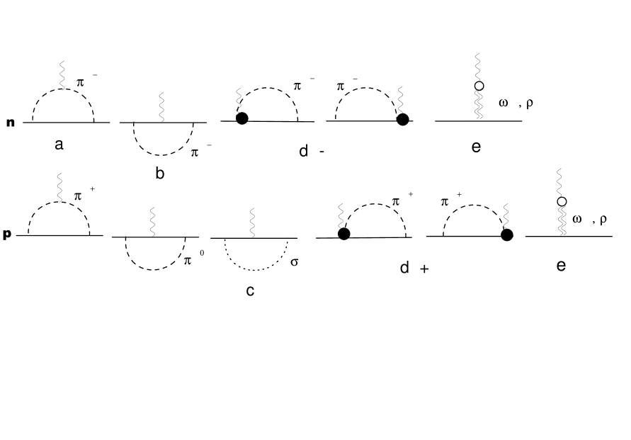
FIG. 1.: Electromagnetic vertex of the nucleon. The first row of diagrams shows the neutron vertex, the second row the proton vertex (without the $\gamma^{\mu}$ term). Dashed lines depict $\pi-$meson, dotted lines $\sigma-$meson, wavy lines photon, double-wavy lines $\omega-$ and $\rho-$mesons, and solid lines nucleon.

FIG. 2.: Left panel: the neutron anomalous magnetic moment as a function of the pion cut-off momentum. Right panel: the proton anomalous magnetic moment versus the mass of the $\sigma-$meson. Experimental values are indicated by the open squares. Various contributions in eqs. (75) and (76) corresponding to the diagrams ‘a,b,c’ and ‘d$\pm$’ in fig. 1 are also shown.

REFERENCES

- [1] B.D. Fried, Phys. Rev. 88, 1142 (1952).
- [2] E.J. Ernst, R.G. Sachs and K.C. Wali, Phys. Rev. 119, 1105 (1960).
- [3] J.D. Walecka, Nuovo Cimento 11, 821 (1959).
- [4] H.W.L. Naus and J.H. Koch, Phys. Rev. C 36, 2459 (1987).
- [5] P.C. Tiemeijer and J.A. Tjon, Phys. Rev. C 42, 599 (1990).
- [6] F. Gross and D.O. Riska, Phys. Rev. C 36, 1928 (1987).
- [7] H.C. Dönges, M. Schäfer and U. Mosel, Phys. Rev. C 51, 950 (1995).
- [8] S. Kondratyuk and O. Scholten, nucl-th/9906044.
- [9] R.M. Davidson, Phys. Rev. C 47, 2492 (1993).
- [10] M. Gell-Mann and M. Lèvy, Nuovo Cimento 16, 705 (1960)
- [11] C. Itzykson and J.-B. Zuber, Quantum Field Theory, (McGraw-Hill Book Company, 1985).
- [12] V. De Alfaro, S. Fubini, G. Furlan and C. Rossetti, Currents in Hadron Physics, (North-Holland Publ. Company, Amsterdam-London, American Elsevier Publ. Company Inc., New York, 1973).
- [13] W. Pauli, Nuovo Cimento 10, 648 (1953).
- [14] M. Chretien and R.E. Peierls, ibid., 668 (1953).
- [15] P. Kristensen and C. Mller, Danske Videnskabernes Selskab, Mat. Fys., Meddelelser 27, N7 (1952).
- [16] G.V. Efimov, Nonlocal Interactions of Quantum Fields (in Russian), (Nauka Publ., Moscow, 1977); Problems of Quantum Theory of Nonlocal Interactions (in Russian), (Nauka Publ., Moscow, 1985).
- [17] R.G.E. Timmermans, Czech. Journ. Phys. 46, 751 (1996).
- [18] J. Rzewuski, Nuovo Cimento 10, 784 (1953).
- [19] C. Bloch, Danske Videnskabernes Selskab, Mat. Fys., Meddelelser 27, N8 (1952).
- [20] A.Yu. Korchin and A.V. Shebeko, Proceedings of the 4th International Conference “Mesons and light nuclei”, Bechyne Castle, ČSSR, 1988, contribution A4, p.22.
- [21] A.Yu. Korchin and A.V. Shebeko, Sov. J. Nucl. Phys. 54, 214 (1991).
- [22] R. Machleidt, K. Holinde and Ch. Elster, Phys. Rep. 149, 1 (1987).
- [23] T. Ericson and W. Weise, Pions and Nuclei, (Clarendon Press, Oxford, 1988), Appendix 7.
- [24] E. Klingle, N. Kaizer and W. Weise, Z. Phys. A 356, 193 (1996).
- [25] S. Nozawa, B. Blankleider and T.-S.H. Lee, Nucl. Phys. A513, 459 (1990); H. Garcilazo and E. Moya de Guerra, Nucl. Phys. A562, 521 (1993).
- [26] T. Feuster and U. Mosel, Phys. Rev. C 59, 460 (1999).
- [27] J. Flender and M.F. Gari, Z. Phys. A 343, 467 (1992).
- [28] Particle Data Group, Review of Particle Physics, Eur. Phys. J. C 15, 1 (2000).
- [29] J.C. Collins, Renormalization, (Cambridge University Press, 1984).