Spin-isospin excitations and $\beta^{+}/EC$ half-lives of medium-mass deformed nuclei

Abstract

A selfconsistent approach based on a deformed HF+BCS+QRPA method with density-dependent Skyrme forces is used to describe $\beta^{+}$-decay properties in even-even deformed proton rich nuclei. Residual spin-isospin forces are included in the particle-hole and particle-particle channels. The quasiparticle basis contains neutron-neutron and proton-proton pairing correlations in the BCS approach, while neutron-proton pairing interaction is treated as a residual force in QRPA. We discuss the sensitivity of Gamow-Teller strength distributions and $\beta^{+}/EC$ half-lives to deformation, pairing and the strength of the particle-particle interaction. The dependence on deformation is also compared to that of spin $M1$ strength distributions.

I Introduction

Exploring the properties of nuclei with unusual proton to neutron ratios is nowadays one of the major tasks and most active topics in nuclear structure physics, both theoretical and experimentally [1]. In this context, the beta-decay properties of these exotic objects are of extreme importance in two different aspects. First, most nuclei of astrophysical interest [2] are those far from stability and their beta-decay rates have to be estimated theoretically. Second, beta-decay properties and nuclear structure are intimately related. It is clear that a precise and reliable description of the ground state of the parent nucleus and of the states populated in the daughter nucleus is necessary to obtain a good description of the $\beta-$strength distribution, and vice versa, failures to describe such distributions would indicate that an improvement of the theoretical formalism is needed.

Microscopic models to describe the $\beta$-strength based on spherical single-particle wave functions and energies with pairing and residual interactions treated in Random Phase Approximation (RPA) or Quasiparticle Random Phase Approximation (QRPA) were first studied in Ref. [3]. Extensions of these models to deal with deformed nuclei were done in Ref. [4], where a Nilsson potential was used to generate single-particle orbitals. Subsequent extensions including Woods-Saxon type potentials [5], residual interactions in the particle-particle channel [6], consistent Hartree-Fock (HF) mean field with residual interactions treated in Tamm Dancoff approximation [7], selfconsistent approaches in spherical neutron-rich nuclei [8] and based on an energy-density functional [9], can be also found in the literature.

In a previous work [10, 11] we studied ground state and $\beta$-decay properties of exotic nuclei on the basis of a deformed selfconsistent HF+BCS+QRPA calculation with density dependent effective interactions of Skyrme type. This is a well founded approach that has been very successful in the description of spherical and deformed nuclei within the valley of stability [12]. In this method once the parameters of the effective Skyrme interaction are determined, basically by fits to global properties in spherical nuclei over the nuclear chart, and the gap parameters of the pairing force are specified, there are no free parameters left. Both the residual interaction and the mean field are consistently obtained from the same 2-body force. This is therefore a reliable method, suitable for extrapolations into the unstable regions approaching the drip lines. It is worth investigating whether these powerful tools designed to account for the properties of stable nuclei are still valid when approaching the drip lines.

The residual interaction introduced in Refs. [10, 11], consistent with the mean field, acts in the particle-hole channel ($ph$). However, it has been pointed out (see for instance Ref. [13] and refs. therein) that for a complete description of the $\beta^{+}$ and $\beta\beta$ strengths, the inclusion of the particle-particle ($pp$) residual interaction is required. We gave in [11] an example of the sensitivity of the results to the inclusion of such a force but a complete calculation within our formalism including this force is still missing. One of the purposes of this work is to extend our previous calculations by including a residual separable force in the $pp$ channel and to study its effect in a systematic way to distinguish what is general and what is particular in the behavior of the nuclear response. To this end we include in the QRPA calculation a separable neutron-proton pairing force as part of the residual interaction.

Following the same criteria as in our previous work [11], we apply this formalism to the study of a series of proton rich isotopes approaching $N=Z$ in the mass region $A=70$. There are several reasons why this is a region of special interest to study $\beta$-decay. One is that the $Q$-value of the decay ($Q_{EC}$) is quite large in proton rich nuclei [14]. This means that a large fraction of the Gamow-Teller (GT) strength is contained within the $Q_{EC}$ window. Therefore, one can investigate directly the structure of the GT strength distribution by $\beta$-decay measurements without dealing with other indirect methods to extract the GT strength such as $(p,n)$ or $(n,p)$ charge exchange reactions. Another aspect to stress is that the mass region $A\simeq 70$ is at the border or beyond the scope of the full shell model calculations. Predictions for the strength distributions, half-lives, and other decay properties obtained from the present formalism are of special relevance in this mass region since they may be at the moment the most reliable calculations. The present results can then be used as a guidance to further experimental searches. It is also worth mentioning that this mass region is known to present particular structure effects, such as shape coexistence, which are the result of a delicate balance of competing nuclear shapes [7, 15]. It is then important to explore whether the dependence of the beta-decay properties on the deformation of the parent nucleus could be used as an additional piece of information to elucidate the shape of the nucleus. As a last point, we mention that, by approaching systematically the $N=Z$ isotopes in various isotopic chains, we are placed in optimum conditions to observe whether agreement with experiment breaks down at some point as we approach $N=Z$. These isotopic chains are a laboratory to test the validity of our formalism and to look for failures related to the appearance of new physics such as neutron-proton pairing correlations not taken into account explicitly in the present mean field calculations, that may be important in $N=Z$ nuclei. In this work we extend the study of Refs. [10, 11] by including a residual neutron-proton pairing interaction in the $J^{\pi}=1^{+}$ channel, by studying the influence of usual BCS pairing correlations in the $N=Z$ isotopes, and by discussing the similarities between the GT strength distributions and the spin $M1$ strength distributions, which are the $\Delta T_{z}=0$ isospin counterparts of the $\Delta T_{z}=\pm 1$ GT transitions.

In Section 2, we present a brief summary containing the basic points in our theoretical description. Section 3 contains the results obtained for the GT strength distributions with a discussion of the dependence on the residual interaction, pairing correlations, and deformation. We also compare our results to the experimental available information. Spin $M1$ strength distributions are studied in Section 4 discussing their analogies with the GT strength distributions. The conclusions are given in Section V.

II Theoretical Approach

In this Section we summarize briefly the theory involved in the microscopic calculations presented in the next Sections. More details can be found in Refs. [10, 11]. Our method consists in a selfconsistent formalism based on a deformed Hartree-Fock mean field obtained with a Skyrme interaction including pairing correlations in the BCS approximation. We consider in this paper the force SG2 [16] of Van Giai and Sagawa, that has been successfully tested against spin and isospin excitations in spherical [16] and deformed nuclei [17]. Comparison to calculations obtained with other Skyrme forces have been made in Refs. [10, 11], showing that the results do not differ in a significant way. The single particle energies, wave functions, and occupations probabilities are generated from this mean field.

For the solution of the HF equations we follow the McMaster procedure that is based in the formalism developed in Ref.[18] as described in Ref.[19]. Time reversal and axial symmetry are assumed. The single-particle wave functions are expanded in terms of the eigenstates of an axially symmetric harmonic oscillator in cylindrical coordinates. We use eleven major shells. The method also includes pairing between like nucleons in the BCS approximation with fixed gap parameters for protons $\Delta_{\pi},$ and neutrons $\Delta_{\nu}$, which are determined phenomenologically from the odd-even mass differences through a symmetric five term formula involving the experimental binding energies [20]. The values used in this work are the same as those given in Ref. [11].

In a previous work [11] we analyzed the energy surfaces as a function of deformation for all the isotopes under study here. For that purpose, we performed constrained HF calculations with a quadrupole constraint [21] and we minimized the HF energy under the constraint of keeping fixed the nuclear deformation. Calculations in this paper are performed for the equilibrium shapes of each nucleus, that is, for the solutions, in general deformed, for which we obtained minima in the energy surfaces. Most of these nuclei present oblate and prolate equilibrium shapes [11] that are very close in energy.

We add to the mean field a spin-isospin residual interaction, which is expected to be the most important residual interaction to describe GT transitions. This interaction contains two parts. The particle-hole part is responsible for the position and structure of the GT resonance [6, 11] and is derived selfconsistently from the same energy density functional (and Skyrme interaction) as the HF equation, in terms of the second derivatives of the energy density functional with respect to the one-body densities [22]. The residual interaction is finally written in a separable form by averaging the Landau-Migdal resulting force over the nuclear volume,

$$V^{ph}_{GT}=2\chi^{ph}_{GT}\sum_{K=0,\pm 1}(-1)^{K}\beta^{+}_{K}\beta^{-}_{-K}\,,$$ (1)

where

$$\beta^{+}_{K}=\sum_{\pi\nu}\left\langle\nu|\sigma_{K}|\pi\right\rangle a^{+}_{\nu}a_{\pi}\,.$$ (2)

The coupling strength is given by [10, 11]

$$\chi^{ph}_{GT}=-\frac{3}{8\pi R^{3}}\left\{t_{0}+\frac{1}{2}k_{F}^{2}\left(t_{1}-t_{2}\right)+\frac{1}{6}t_{3}\rho^{\alpha}\right\}$$ (3)

and it is completely determined by the Skyrme parameters $t_{0},t_{1},t_{2},t_{3},\alpha$, the nuclear radius $R$, and the Fermi momentum $k_{F}$, obtained with the same Skyrme force for the given nucleus.

The particle-particle part is a neutron-proton pairing force in the $J^{\pi}=1^{+}$ coupling channel. We introduce this interaction in the usual way [6, 13, 23], that is, in terms of a separable force with a coupling constant $\kappa^{pp}_{GT}$, which is fitted to the phenomenology,

$$V^{pp}_{GT}=-2\kappa^{pp}_{GT}\sum_{K}(-1)^{K}P^{+}_{K}P_{-K}\,,$$ (4)

where

$$P^{+}_{K}=\sum_{\pi\nu}\left\langle\pi\left|\left(\sigma_{K}\right)^{+}\right|\nu\right\rangle a^{+}_{\nu}a^{+}_{\bar{\pi}}\,.$$ (5)

The two forces $ph$ and $pp$ in Eqs. (1) and (4) are defined with a positive and a negative sign, respectively, according to their repulsive and attractive character, so that the coupling strengths $\chi$ and $\kappa$ take positive values.

The peak of the GT resonance is almost insensitive to the $pp$ force and $\kappa^{pp}_{GT}$ is usually adjusted to reproduce the half-lives [6]. However, one should be careful with the choice of this coupling constant. Since the $pp$ force is introduced independently of the mean field, if $\kappa^{pp}_{GT}$ is strong enough it may happen that the QRPA collapses, because the condition that the ground state be stable against the corresponding mode is not fulfilled. This happens because the $pp$ force, being an attractive force, makes the GT strength to be pushed down to lower energies with increasing values of $\kappa^{pp}_{GT}$.

A careful search of the optimal strength can certainly be done for each particular case, but this is not our purpose here. Instead, we have chosen the same coupling constant for all nuclei considered here. This value has been obtained under the requirements of improving in general the agreement with the experimental half-lives while being still far from the values leading to the collapse. This will be discussed in more detail in the next Section.

The proton-neutron quasiparticle random phase approximation (QRPA) phonon operator for GT excitations in even-even nuclei is written as

$$\Gamma_{\omega_{K}}^{+}=\sum_{\pi\nu}\left[X_{\pi\nu}^{\omega_{K}}\alpha_{\nu}^{+}\alpha_{\bar{\pi}}^{+}+Y_{\pi\nu}^{\omega_{K}}\alpha_{\bar{\nu}}\alpha_{\pi}\right]\,,$$ (6)

where $\alpha^{+}\left(\alpha\right)$ are quasiparticle creation (annihilation) operators, $\omega_{K}$ are the excitation energies, and $X_{\pi\nu}^{\omega_{K}},Y_{\pi\nu}^{\omega_{K}}$ the forward and backward amplitudes, respectively. The equations of motion are solved in the proton-neutron QRPA.

From the QRPA equations the forward and backward amplitudes are obtained as [23]

$$X_{\pi\nu}^{\omega_{K}}=\frac{1}{\omega_{K}-\varepsilon_{\pi\nu}}\left[2\chi^{ph}_{GT}\left(a_{\pi\nu}M_{-}^{\omega_{K}}+b_{\pi\nu}M_{+}^{\omega_{K}}\right)-2\kappa^{pp}_{GT}\left(c_{\pi\nu}M_{--}^{\omega_{K}}+d_{\pi\nu}M_{++}^{\omega_{K}}\right)\right]\,,$$ (7)

$$Y_{\pi\nu}^{\omega_{K}}=\frac{1}{\omega_{K}+\varepsilon_{\pi\nu}}\left[2\chi^{ph}_{GT}\left(a_{\pi\nu}M_{+}^{\omega_{K}}+b_{\pi\nu}M_{-}^{\omega_{K}}\right)+2\kappa^{pp}_{GT}\left(c_{\pi\nu}M_{++}^{\omega_{K}}+d_{\pi\nu}M_{--}^{\omega_{K}}\right)\right]\,,$$ (8)

with $\varepsilon_{\pi\nu}=E_{\nu}+E_{\pi}$ the two-quasiparticle excitation energy in terms of the quasiparticle energies $E_{i}$. $M^{\omega_{K}}$ are given by

$$M_{-}^{\omega_{K}}=\sum_{\pi\nu}\left(a_{\pi\nu}X_{\pi\nu}^{\omega_{K}}-b_{\pi\nu}Y_{\pi\nu}^{\omega_{K}}\right)\,,$$ (9)

$$M_{+}^{\omega_{K}}=\sum_{\pi\nu}\left(b_{\pi\nu}X_{\pi\nu}^{\omega_{K}}-a_{\pi\nu}Y_{\pi\nu}^{\omega_{K}}\right)\,,$$ (10)

$$M_{--}^{\omega_{K}}=\sum_{\pi\nu}\left(c_{\pi\nu}X_{\pi\nu}^{\omega_{K}}+d_{\pi\nu}Y_{\pi\nu}^{\omega_{K}}\right)\,,$$ (11)

$$M_{++}^{\omega_{K}}=\sum_{\pi\nu}\left(d_{\pi\nu}X_{\pi\nu}^{\omega_{K}}+c_{\pi\nu}Y_{\pi\nu}^{\omega_{K}}\right)\,,$$ (12)

with

$$a_{\pi\nu}=v_{\nu}u_{\pi}\Sigma_{K}^{\nu\pi};\ \ \ b_{\pi\nu}=u_{\nu}v_{\pi}\Sigma_{K}^{\nu\pi};\ \ \ c_{\pi\nu}=u_{\nu}u_{\pi}\Sigma_{K}^{\nu\pi};\ \ \ d_{\pi\nu}=v_{\nu}v_{\pi}\Sigma_{K}^{\nu\pi}\,,$$ (13)

where $v^{\prime}$s are occupation amplitudes ($u^{2}=1-v^{2}$) and $\Sigma_{K}^{\nu\pi}$ spin matrix elements connecting neutron and proton states with spin operators

$$\Sigma_{K}^{\nu\pi}=\left\langle\nu\left|\sigma_{K}\right|\pi\right\rangle\,.$$ (14)

The solution of the QRPA equations can be found solving first a dispersion relation, which is now of fourth order in the excitation energies $\omega$. Then, for each value of the energy the amplitudes $M$ are determined by using the normalization condition of the phonon amplitudes

$$\sum_{\pi\nu}\left[\left(X_{\pi\nu}^{\omega_{K}}\right)^{2}-\left(Y_{\pi\nu}^{\omega_{K}}\right)^{2}\right]=1\,.$$ (15)

The technical procedure to solve these QRPA equations is well described in Ref. [23].

In the intrinsic frame the GT transition amplitudes connecting the QRPA ground state $\left|0\right\rangle\ \ \left(\Gamma_{\omega_{K}}\left|0\right\rangle=0\right)$ to one phonon states $\left|\omega_{K}\right\rangle\ \ \left(\Gamma^{+}_{\omega_{K}}\left|0\right\rangle=\left|\omega_{K}\right\rangle\right)$, are given by

$$\left\langle\omega_{K}|\sigma_{K}t^{\pm}|0\right\rangle=\mp M^{\omega_{K}}_{\pm}\,.$$ (16)

The Ikeda sum rule is always fulfilled in our calculations

$$\sum_{\omega}\left[\left(M^{\omega}_{-}\right)^{2}-\left(M^{\omega}_{+}\right)^{2}\right]=3(N-Z)\,.$$ (17)

III Decay properties

The bulk properties of the isotope chains considered here were already studied in Ref. [11]. Binding energies, charge radii, quadrupole moments, and moments of inertia were discussed and compared successfully to available experimental data. Here we will concentrate on the decay properties.

In this Section we discuss the results obtained for the GT strength distributions, half-lives, and summed strengths in the proton rich isotopes belonging to the $A\simeq 70$ mass region. The results correspond to QRPA calculations with the Skyrme force SG2 and they have been performed for the nuclear shapes that minimize the HF energy.

Figures showing the GT strength distributions are plotted versus the excitation energy of daughter nucleus. The distributions of the GT strength have been folded with $\Gamma=1$ MeV width Gaussians to facilitate the comparison among the various calculations, so that the original discrete spectrum is transformed into a continuous profile. These distributions are given in units of $g_{A}^{2}/4\pi$ and one should keep in mind that a quenching of the $g_{A}$ factor, typically $g_{A,eff}=(0.7-0.8)\ g_{A,free}$ is expected on the basis of the observed quenching in charge exchange reactions and spin $M1$ transitions in stable nuclei, where $g_{s,eff}$ is also known to be approximately $0.7\ g_{s,free}$. Therefore, a reduction factor of about two is expected in these strength distributions in order to compare with experiment. This factor is of course taken into account when comparing to experimental half-lives.

A The role of the residual interactions

Figure 1 illustrates the effect of the residual interactions on the uncorrelated 2-quasiparticle calculation. The calculations are done for the oblate and prolate shapes of ⁷⁴Kr. The coupling strength of the $ph$ residual interaction $\chi^{ph}_{GT}$ is obtained from Eq. (3), and its value for $A=74$ and Skyrme force SG2 is $\chi^{ph}_{GT}=0.37$ MeV. The coupling strength of the $pp$ residual interaction is varied from $\kappa^{pp}_{GT}=0$ to $\kappa^{pp}_{GT}=0.07$ MeV.

If we compare first the calculation with only the $ph$ residual interaction (dotted line) to the uncorrelated one (thin solid line), we can see that the repulsive $ph$ force introduces two types of effects. One is a shift of the GT strength to higher excitation energies with the corresponding displacement of the position of the GT resonance. The other is a reduction of the total GT strength. Obviously these effects are more pronounced as we increase the value of the coupling strength $\chi^{ph}_{GT}$. If we now introduce a $pp$ residual interaction (dashed and solid lines), we can see that its effect, being an attractive force, is to shift the strength to lower excitation energies, reducing the total GT strength as well. The shift and reduction of strength is more pronounced at high excitation energies and the position of the GT resonance is hardly affected by this interaction. The GT strength is also pushed a bit by the $pp$ interaction to lower energies in the low energy excitation region. This effect, although small, is of great relevance in the calculation of the $\beta^{+}/EC$ half-lives, which are only sensitive to the distribution of the strength contained in the energy region below the $Q_{EC}$ window. By comparing the curves obtained from $\kappa^{pp}_{GT}=0.05$ MeV (dashed line) and $\kappa^{pp}_{GT}=0.07$ MeV (solid line), we can also see how these effects are more pronounced as we increase the value of the coupling strength.

This is the reason why the usual procedure to fit these two coupling strengths $\chi^{ph}_{GT}$ and $\kappa^{pp}_{GT}$ is as follows: First one chooses $\chi^{ph}_{GT}$ to reproduce the position of the GT resonance, usually determined from charge exchange reactions $(p,n)$ and $(n,p)$, and then one chooses $\kappa^{pp}_{GT}$ to reproduce the half-life. In our work, since the value of $\chi^{ph}_{GT}$ is determined selfconsistently and the known GT resonances are reasonably well described [11], we do not carry out this case by case fitting procedure. However, to determine the value of $\kappa^{pp}_{GT}$, we calculate first GT strength distributions and half-lives and compare the latter with experiment to extract a value that producing a reasonable agreement is still within the range of values compatible with the correct treatment of the QRPA.

In Figure 2 we can see the result of the calculation of the half-lives in ⁷⁶Sr as a function of the coupling strength $\kappa^{pp}_{GT}$. The half-lives are obtained from the familiar expression,

$$T_{1/2}^{-1}=\frac{A^{2}}{D}\sum_{\omega}f\left(Z,\omega\right)\left|\left\langle 1_{\omega}^{+}\left\|\beta^{+}\right\|0^{+}\right\rangle\right|^{2}\,,$$ (18)

where $f\left(Z,\omega\right)$ are the Fermi integrals. Note that in our previous work [11], we used for these integrals the values tabulated in [24]. In the present calculations we compute the Fermi integrals numerically for each $Z,\omega$ values. By this procedure we get more accurate results.

We use $D=6200$ s and include standard effective factors

$$A^{2}=\left[\left(g_{A}/g_{V}\right)_{eff}\right]^{2}=\left[0.77\left(g_{A}/g_{V}\right)_{free}\right]^{2}=0.90\,.$$ (19)

The half-life decreases with increasing values of $\kappa^{pp}_{GT}$. This is clear because as $\kappa^{pp}_{GT}$ increases the strength becomes more concentrated at low excitation energies below $Q_{EC}$ and therefore the half-lives are smaller. This is true up to values around $\kappa^{pp}_{GT}=0.1$ MeV, where the collapse of the QRPA takes place. In the case of ⁷⁶Sr, we get an optimum value of $\kappa^{pp}_{GT}=0.03$ MeV and $\kappa^{pp}_{GT}=0.07$ MeV for the oblate and prolate shapes, respectively. This value will of course depend, among other factors, on the nucleus, shape, and Skyrme interaction and a case by case fitting procedure could be carried out. Nevertheless, we have done calculations for other cases and found that, in general, values around $\kappa^{pp}_{GT}=0.07$ MeV improve the agreement with experiment in most cases and since this is a valid value far from collapse, we have chosen $\kappa^{pp}_{GT}=0.07$ MeV as the value of the coupling constant of the $pp$ residual interaction.

In Ref. [6] Homma and collaborators studied $\beta-$decay properties using Nilsson+BCS+QRPA with $ph$ and $pp$ separable residual interactions. They considered a wide range of nuclei to extract phenomenologically the coupling strength of such residual interactions by fits to experimental half-lives. They obtained the following dependence on the mass number: $\chi^{ph}_{GT}=5.2/A^{0.7}$ MeV, $\kappa^{pp}_{GT}=0.58/A^{0.7}$ MeV. For $A=70$ this gives a $ph$ strength $\chi^{ph}_{GT}=0.27$ MeV and a $pp$ strength $\kappa^{pp}_{GT}=0.03$ MeV. The $ph$ strength is somewhat smaller than the one obtained from Eq. (3), derived selfconsistently from our mean field. The $pp$ strength is also smaller than the value adopted here. This is consistent with the trend observed in Fig. 1 of Homma et al. [6] that shows that for decreasing values of $\chi^{ph}_{GT}$ one needs smaller values of $\kappa^{pp}_{GT}$. On the other hand, a discussion of the adequacy of our $ph$ strength is also demonstrated in Ref. [11], where we compared our results on the position of the GT resonance with experimental data from $(p,n)$ and $(n,p)$ reactions in this mass region. The fact that our $ph$ and $pp$ strengths are somewhat different from those in Ref. [6] is not surprising since the mean fields are also different.

B The role of BCS correlations

As already mentioned in the Introduction, our theoretical treatment does not explicitly include neutron-proton pairing correlations in the mean field. Thus, our quasiparticle basis only includes neutron-neutron and proton-proton pairing correlations in the BCS approach. In principle, one could extend the BCS treatment to include also neutron-proton pairing correlations in the mean field. This may be important particularly for N=Z nuclei.

In Ref. [11] we studied bulk properties (binding energies, charge radii, quadrupole moments, moments of inertia,…) of the nuclei considered here and found that the agreement between theory and experiment is as good for the $N=Z$ as for the $N=Z+2,Z+4,Z+6$ isotopes. We concluded that the effect of neutron-proton pairing correlations on these bulk properties is roughly taken into account by the use of the phenomenological gap parameters $\Delta_{\pi},\Delta_{\nu}.$

The main effect of taking into account neutron-proton pairing in the HF+BCS calculation would be to increase the diffuseness of the Fermi surface [25]. This diffuseness is proportional to the gap parameters. It is therefore interesting to study the sensitivity of the GT strength to the gap parameters in the $N=Z$ nuclei ⁶⁴Ge, ⁶⁸Se, ⁷²Kr, and ⁷⁶Sr. To this end we compare in Fig. 3 the QRPA results obtained with the SG2 force in those nuclei for various values of the gap parameters differing by $\pm 0.5$ MeV from the values extracted from the phenomenology. To make the discussion easier we did not include the $pp$ residual interaction in those figures.

The main effect of the BCS correlations is to create new transitions that were forbidden in the absence of such correlations. Since the occupation probabilities are now different from 0 or 1, the already existing peaks at $\Delta=0$ will decrease when $\Delta>0$, while new strength will appear at other energies and will increase with increasing gap parameters. This new strength is in general located at high excitation energy, while the strength already present at $\Delta=0$ is mainly concentrated at lower energy. As a consequence, the main effect of increasing the Fermi diffuseness is to smooth out the profile of the GT strength distribution, increasing the strength at high energies and decreasing the strength at low energies.

It is clear from Fig. 3 that each particular case has its own peculiarities but the general trend described above plays the major role. It is also interesting to remark that in the high energy tail beyond the GT resonance, the effects of increasing $\Delta$ and increasing $\kappa^{pp}_{GT}$ are opposite. As we mentioned before, increasing $\kappa^{pp}_{GT}$ tends to deplete those tails.

C The role of deformation

The role of deformation on the GT strength distributions can be summarized, in general, in two types of effects. First, deformation breaks down the degeneracy of the spherical shells and this implies that the GT strength distributions corresponding to deformed nuclear shapes will be much more fragmented than the corresponding spherical ones. Second, the energy levels of deformed orbitals coming from different spherical shells cross each other in a way that depends on the magnitude of the quadrupole deformation as well as on the oblate or prolate character. This level crossing may lead in some instances to similar profiles in the GT strength distributions of the various coexisting nuclear shapes but in other cases it may lead to sizeable differences between the GT strength distributions corresponding to different shapes of the same parent nucleus. This fact can be exploited to gain information on what is the nuclear shape of a nucleus by just looking at the structure of its $\beta$-decay.

Fig. 4 summarizes the main results of this work. They correspond to the GT strength distributions obtained from our HF+BCS+QRPA with SG2 in the isotope chains of Ge, Se, Kr, and Sr. We can see in this figure the results obtained for the possible nuclear shapes of the isotopes ranging from $N=Z$ to $N=Z+6$. As usual the strengths are in units of $g_{A}^{2}/4\pi$ and are plotted versus the excitation energy of the daughter nucleus.

We can see that in general the $N=Z$ isotopes of each chain contain the maximum strength as it corresponds to the most unstable nuclei. This strength becomes smaller and smaller as we increase the number of neutrons approaching the stable isotopes. The excitation energy of the GT resonance also decreases with the number of neutrons.

If we look in Fig. 3 the case of Ge and Se isotopes, we can see that there are no signatures of the actual character, oblate or prolate, of the deformation of the parent nucleus: Both equilibrium shapes produce similar GT profiles independently of whether it is oblate or prolate. Then, it can be concluded that in these isotopes one cannot use GT distributions to distinguish between the two coexistent shapes predicted by the theory. On the other hand, the figures corresponding to Kr and Sr isotopes, show differences in the GT profiles of the various shapes for each isotope that can be easily identified even within the $Q_{EC}$ window. A case by case analysis allows one to conclude that the most favorable candidates to look for deformation effects based on $\beta$-decay measurements are ⁷⁴Kr and ^76,78,80Sr. In these isotopes the GT strengths within the $Q_{EC}$ window are different enough to distinguish between different equilibrium shapes. On the contrary, there are cases like ⁷²Kr where though the large $Q_{EC}$ value ($Q_{EC}=5$ MeV) make it worth to investigate experimentally, the measured strength may not be conclusive on the shape because oblate and prolate shapes produce similar profiles. Other isotopes like ^76,78Kr have small $Q_{EC}$ values that will not allow a clear conclusion either, while ⁷⁴Kr seems to be the best Kr candidate. It has a $Q_{EC}$ window (3.1 MeV) big enough to distinguish between a continuously increasing profile, as the prolate shape predicts, or a completely developed bump structure peaked at around 1.5 MeV and vanishing at about the $Q_{EC}$ value, as the oblate shape predicts. A similar situation happens in the case of ⁷⁶Sr ($Q_{EC}=6.1$ MeV). The oblate shape produces a peak centered at around 1 MeV and a second one centered at 6 MeV, while the prolate shape produces a GT distribution that increases almost continuously up to 6 MeV. The case of ⁷⁸Sr ($Q_{EC}=3.8$ MeV) is again a clear case where one can distinguish between the bump structure generated by the spherical shape or the continuously increasing pattern of the prolate case. The same is true for the ⁸⁰Sr isotope, although in this case $Q_{EC}$ is not so big ($Q_{EC}=1.9$ MeV).

D Comparison to experiment

In this subsection we compare to experiment our calculated $Q_{EC}$ and total $\beta^{+}/EC$ half-lives $T_{1/2}$, as well as a few cases where the GT strength distribution have been partially measured by $\beta$-decay. We also discuss the GT strengths contained within the $Q_{EC}$ windows. The difference with respect to the values quoted in our previous work [11] is that now the $pp$ interaction is included. There is also a minor difference in the calculation of $Q_{EC}$,

$$Q_{EC}=m_{\pi}-m_{\nu}+m_{e}-\left(\lambda_{\nu}+E_{\nu}\right)_{\left(N,Z\right)}+\left(\lambda_{\pi}-E_{\pi}\right)_{\left(N,Z-2\right)}\,.$$ (20)

The $Q_{EC}$ values in Tables 1-4 of Ref. [11] were calculated approximating the lowest quasiparticle energies $E_{\nu}$ and $E_{\pi}$ by the gap parameters $\Delta_{\nu}$ and $\Delta_{\pi}$, respectively, while $Q_{EC}$ values in Table 1 here are calculated using their actual values $E=\sqrt{\left(\epsilon-\lambda\right)^{2}+\Delta^{2}}$.

We can see in Table 1 these results obtained from QRPA calculations with the Skyrme force SG2 and for the different shapes, oblate, prolate or spherical, where the minima occur for each isotope. We did not include the stable nuclei, all having $Q_{EC}$ less than zero and infinite half-lives. It should also be mentioned that the total GT strength below $Q_{EC}$ has been reduced by a quenching factor 0.6 to be consistent with the same quenching used in the calculation of the half-lives in Eq. (18).

We get a very good agreement with the measured $Q_{EC}$ values in practically all cases and the values obtained with the various shapes are quite similar. The half-lives are also well reproduced in most cases. Only in the most stable isotopes, where the half-lives are very large, we find some noticeable discrepancies but this is not so relevant because in these cases the $Q_{EC}$ values are very small and therefore, the half-lives are only sensitive to a tiny region of the GT tail at low energies. In other cases the agreement is very reasonable. The sums of the GT strength up to the $Q_{EC}$ value do not differ much from one shape to another although this does not mean that the structure of the profiles are equivalent. As we have seen in the last subsection, there are cases, ⁷⁴Kr and ^76,78,80Sr, whose profiles can be easily distinguished although the final summed strength is very similar.

Table 2 contains experimental information on GT summed strengths in the $N=Z$ nuclei ⁷²Kr [26] and ⁷⁶Sr [27] up to different values of the excitation energy, always below $Q_{EC}$. They are compared to our theoretical calculations for the two equilibrium shapes using the same quenching factor as in Eq. (19). From this comparison an oblate shape for ⁷²Kr and a prolate shape for ⁷⁶Sr seems to be favored, but this is not yet sufficient for a conclusive answer.

In any case it would be worth to extend the measurements in ⁷⁶Sr to higher excitation energies because it is a very good example where deformation effects are visible (see Fig. 4 for ⁷⁶Sr). On the other hand, the extension of these measurements to the case of ⁷²Kr may not be so relevant since one could not distinguish one shape from another (see Fig. 4 for ⁷²Kr).

IV Magnetic properties

The spin $M1$ transitions are the $\Delta T_{z}=0$ isospin counterparts of the $\Delta T_{z}=\pm 1$ GT transitions. The study carried out in [17] for several isotope chains showed that the $M1$ strength depends on deformation, not only for orbital but also for spin excitations. Thus, on general grounds, one may argue that the deformation dependence of the GT strength discussed earlier should be comparable to that of the spin $M1$ strength considered in [17]. This is expected to be particularly the case when $N=Z$.

In a similar way to Fig. 4 for the GT distributions, we show in Fig. 5 the profiles of the spin $M1$ strength distributions for the same isotope chains. The results correspond to the selfconsistent HF+BCS+QRPA calculations with the SG2 interaction. The details of these calculations are described in [17] and closely follow those of the GT strength except for the $\Delta T_{z}=0$ character of the $M1$ operator.

Similarly to the GT strength distributions in the Ge and Se isotope chains in Fig. 4, we can see that the $B_{\sigma}(M1)$ strength distributions for these two isotopes in Fig. 5 have similar structures for the oblate and prolate shapes. They have a big resonance located at the same energy around 10 MeV and a small bump at about 5 MeV. However, the strength contained in the prolate peak is always larger than the oblate one, contrary to what happened with the GT strengths that were comparable. The spherical shape in ⁷⁴Se produces much less strength than the deformed shapes. We can also see in Fig. 5 for Kr and Sr isotopes that the profiles of the $M1$ strengths corresponding to the prolate and oblate distributions can be clearly distinguished, similarly to the case of the GT distributions in Fig. 4. The strength corresponding to the prolate shape is again the largest. Therefore, clear similarities between the GT and $M1$ strength distributions are observed, but some differences can be seen as well. In particular, for spin $M1$ strength distributions the position and strength of the resonance are practically the same in all nuclei in a given isotope chain. This is different to what happened with the GT strength distributions, where the $\beta^{+}$-GT strength decreases very fast with increasing $N-Z$ due to Pauli blocking, while $M1$ strengths are not affected by this.

V Conclusions

We studied $\beta^{+}$-decay in various isotopic chains of medium-mass proton-rich nuclei within the framework of the selfconsistent deformed HF+BCS+QRPA with Skyrme interactions. Our spin-isospin residual interaction contains a particle-hole part, which is derived selfconsistently from the Skyrme force, and a particle-particle part, which is a separable force representing a neutron-proton pairing force. Compared to previous calculations, where the latter residual interaction was not considered, we obtain in general better agreement with experiment for half-lives. It is worth mentioning that for the N=Z isotopes this agreement is comparable to that achieved for the other isotopes with an excess of neutrons. This indicates that using the phenomenological gap values for neutrons and protons, as well as the neutron-proton pairing correlations as a residual force in QRPA, is sufficient to account at least for this experimental information.

From our study of the dependence on the shape of the GT strength distributions we conclude that there are some interesting cases that are worth to explore experimentally such as ⁷⁴Kr and ^76,78,80Sr. In these examples the measured $\beta^{+}$ strengths below $Q_{EC}$ could be used to identify their equilibrium shapes. In particular, we have observed in ⁷⁶Sr various compatible indications pointing out towards the same conclusion: a strong prolate component in the ground state that is suggested from the comparison to experiment of half-lives and GT strength measured at low excitation energies. Nevertheless, more experimental information is still needed to reach a conclusive answer.

We also studied the energy distributions of the spin $M1$ strength and the similarities and differences with their GT counterparts. We conclude that the main features of GT and spin $M1$ strength distributions are similar. This suggests that we may learn about properties that are observable in highly unstable nuclei (like $\beta$ decay) from properties that are observable in stable nuclei (like $M1$’s), and vice versa. Information on spin $M1$ excitations can be extracted from both leptonic and hadronic probes. In stable nuclei, the combined analysis of electron, photon, and proton scattering data has provided reliable information on orbital and spin $M1$ strength distributions [28]. In principle, the same type of experiments could be performed on the proton rich nuclei considered here. Inelastic $(p,p^{\prime})$ scattering experiments might be particularly suitable to explore the spin part of the $M1$ strength and to test the predictions of the present paper.

Acknowledgments

This work was supported by DGESIC (Spain) under contract number PB98-0676. One of us (A.E.) thanks Ministerio de Educación y Cultura (Spain) for support.

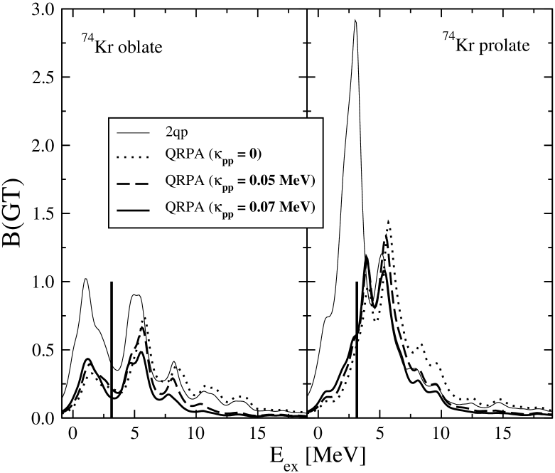
FIG. 1.: GT strength distributions [$g_{A}^{2}/4\pi$] in ⁷⁴Kr plotted versus the excitation energy of the daughter nucleus. Calculations are done in QRPA with the force SG2 for various values of the coupling strength $\kappa^{pp}_{GT}$ of the particle-particle force. Vertical lines indicate experimental $Q_{EC}$ values (see Table 1 for the theoretical $Q_{EC}$ values).

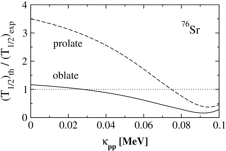
FIG. 2.: Ratios of calculated to experimental half-lives in ⁷⁶Sr as a function of the coupling strength $\kappa^{pp}_{GT}$ of the particle-particle force.

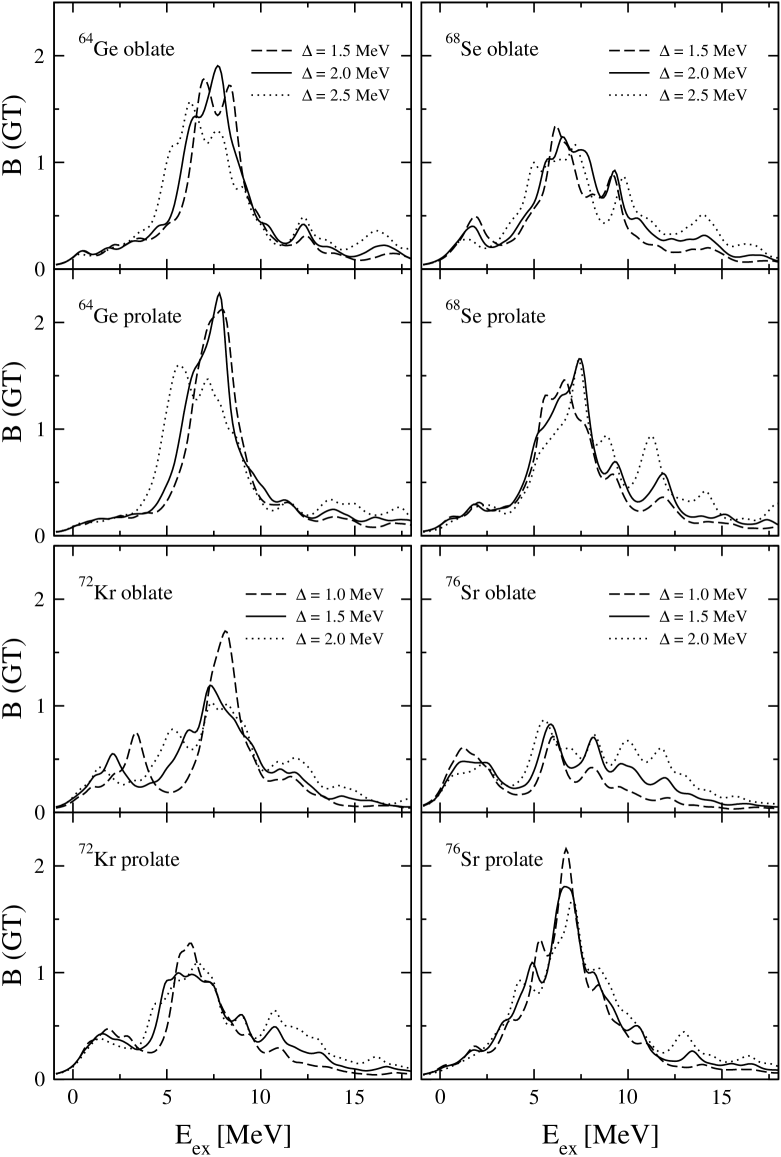
FIG. 3.: Pairing effect in the QRPA Gamow-Teller strength distribution in the $N=Z$ isotopes ⁶⁴Ge, ⁶⁸Se, ⁷²Kr, and ⁷⁶Sr. Solid lines correspond to calculations with empirical pairing gaps, dotted (dashed) lines correspond to calculations with empirical gaps plus (minus) 0.5 MeV.

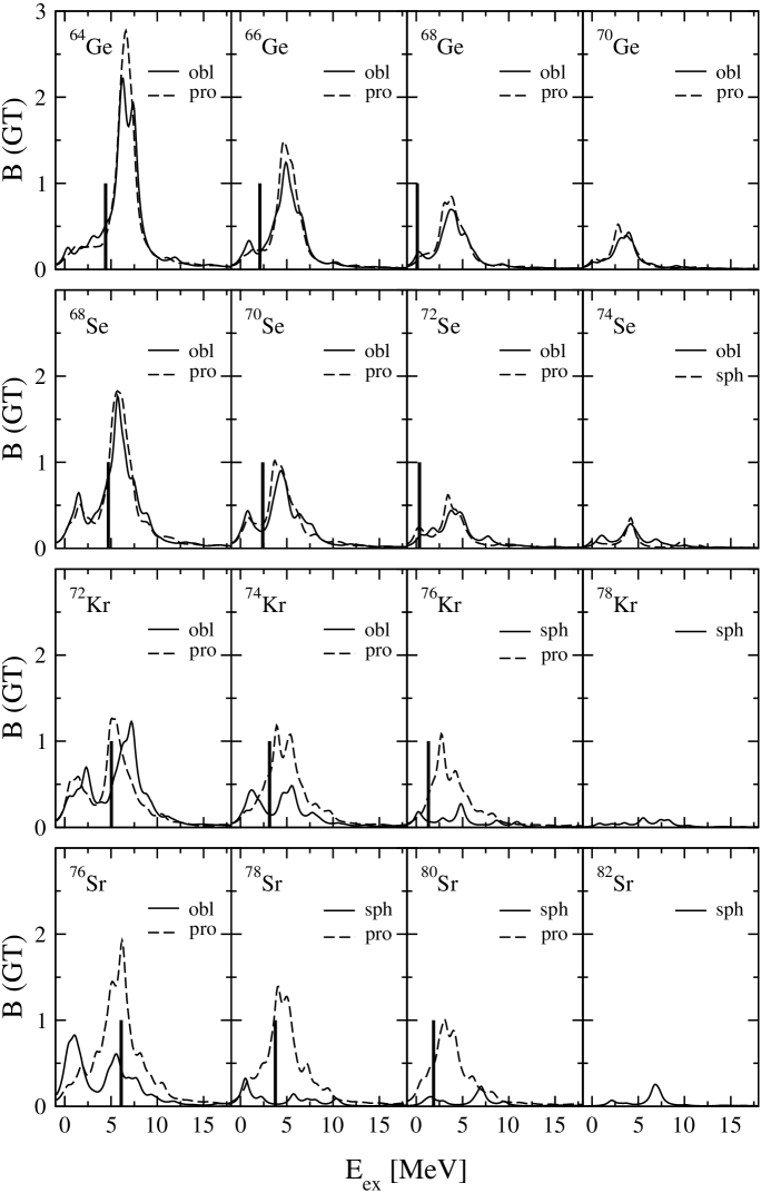
FIG. 4.: Gamow-Teller strength distributions [$g_{A}^{2}/4\pi$] as a function of the excitation energy of the daughter nucleus [MeV]. The results are for the force SG2 in QRPA and for the various shapes of the isotopes ^64,66,68,70Ge, ^68,70,72,74Se, ^72,74,76,78Kr, and ^76,78,80,82Sr. Vertical lines indicate experimental $Q_{EC}$ values (see Table 1 for the theoretical $Q_{EC}$ values).

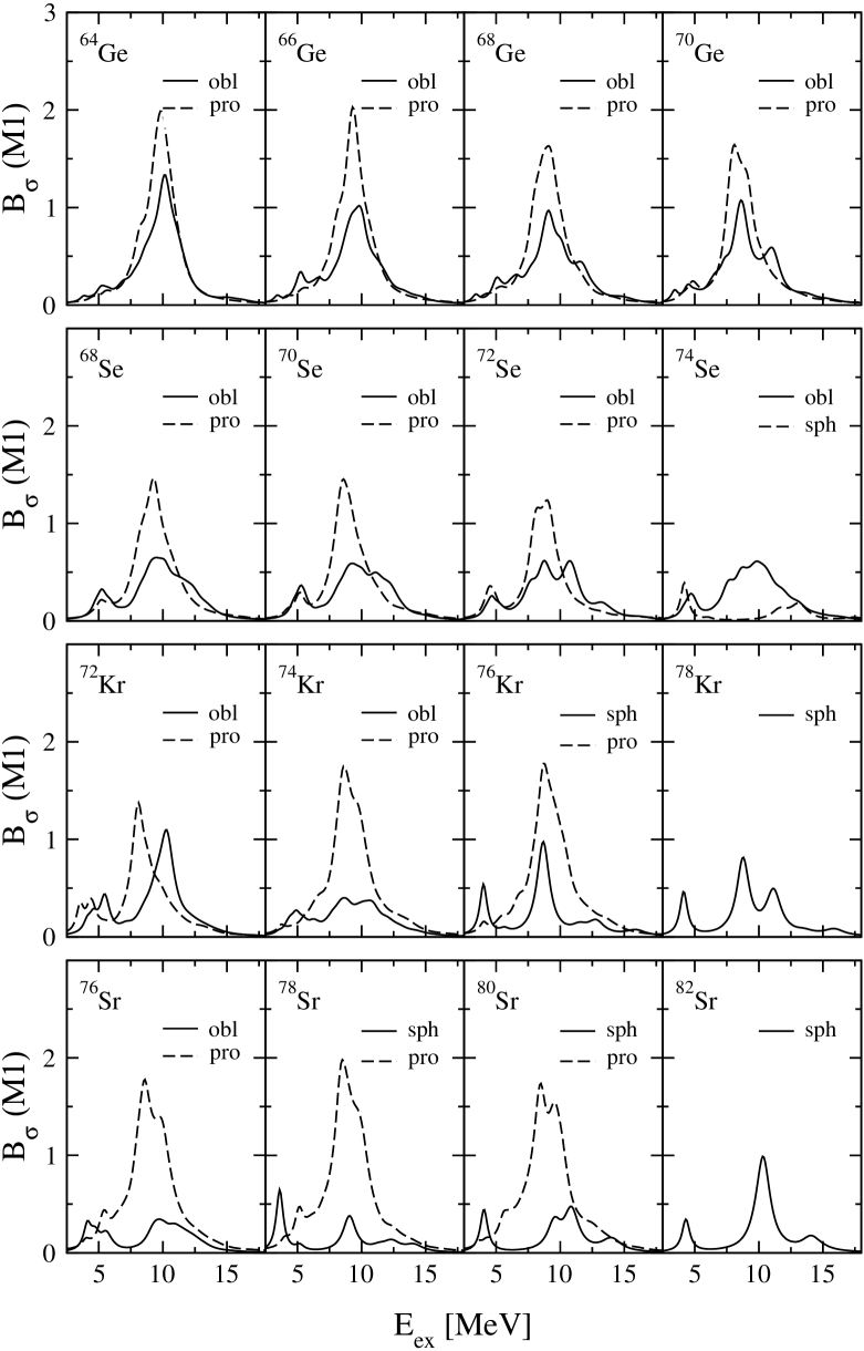
FIG. 5.: Spin $M1$ strength distributions [$\mu_{N}^{2}$] calculated in QRPA with the force SG2. The results are for the various shapes of the isotopes ^64,66,68,70Ge, ^68,70,72,74Se, ^72,74,76,78Kr, and ^76,78,80,82Sr.

Table 1. Results for $Q_{EC}$ values, half-lives $(T_{1/2})$, and GT strength summed up to $Q_{EC}$ energies $(\sum_{Q_{EC}})$. The results correspond to QRPA calculations performed with the Skyrme force SG2 in four isotopic chains and are calculated for the various equilibrium shapes in each nucleus. Experimental values for $Q_{EC}$ and $T_{1/2}$ are from [20].

		$Q_{EC}$			$T_{1/2}$			$\sum_{Q_{EC}}B(GT)$
		exp	th		exp	th
64Ge	obl	4.41	4.3		63.7 s	84.5 s		0.7
	pro		4.1			167.0 s		0.5
66Ge	obl	2.10	2.3		2.3 h	1.6 h		0.3
	pro		2.2			3.1 h		0.2
68Ge	obl	0.11	0.2		271 d	198 d		0.1
	pro		0.3			100 d		0.0
68Se	obl	4.70	4.4		35.5 s	77.2 s		1.1
	pro		4.5			66.4 s		0.9
70Se	obl	2.40	2.5		41.1 m	38.8 m		0.5
	pro		2.7			33.5 m		0.5
72Se	obl	0.34	0.8		8.4 d	3.3 d		0.1
	pro		1.3			0.3 d		0.2
72Kr	obl	5.04	5.0		17.2 s	21.4 s		1.2
	pro		5.2			13.6 s		1.9
74Kr	obl	3.14	3.4		11.5 m	8.7 m		0.7
	pro		3.5			12.4 m		0.6
76Kr	sph	1.31	1.7		14.8 h	4.1 h		0.2
	pro		1.2			38.0 h		0.1
76Sr	obl	6.10	5.9		8.9 s	3.2 s		2.1
	pro		5.8			10.9 s		2.3
78Sr	sph	3.76	4.3		2.7 m	1.3 m		0.4
	pro		3.1			19.9 m		0.6
80Sr	sph	1.87	1.8		1.8 h	56.0 h		0.1
	pro		1.6			6.4 h		0.2

Table 2. Comparison of the GT strengths contained below some given excitation energy between experimental measurements ([26] for ⁷²Kr, [27] for ⁷⁶Sr) and theoretical calculations.

	exp	oblate	prolate
72Kr ($E_{ex}\leq$ 1.836 MeV)	0.5 (1)	0.5	0.8
76Sr ($E_{ex}\leq$ 2.882 MeV)	0.6 – 0.8	1.3	0.6

REFERENCES

- [1] C. Détraz and D.J. Vieira, Annu. Rev. Nucl. Part. Sci. 39 (1989) 407; A. Mueller and B.M. Sherrill, Annu. Rev. Nucl. Part. Sci. 43 (1993) 529; NuPECC report on Nuclear Structure under Extreme Conditions of Isospin, Mass, Spin and Temperature, A.C. Mueller et al. (1997).
- [2] NuPECC report on Nuclear and Particle Astrophysics, F.K. Thielemann et al. (1998); M. Arnould and K. Takahashi, Rep. Prog. Phys. 62 (1999) 395.
- [3] I. Hamamoto, Nucl. Phys. 62 (1965) 49; J.A. Halbleib and R.A. Sorensen, Nucl. Phys. A 98 (1967) 542; J. Randrup, Nucl. Phys. A207 (1973) 209.
- [4] J. Krumlinde and P. Möller, Nucl. Phys. A 417 (1984) 419.
- [5] P. Moller and J. Randrup, Nucl. Phys. A514 (1990) 1.
- [6] M. Hirsch, A. Staudt, K. Muto and H.V. Klapdor-Kleingrothaus, Nucl. Phys. A535 (1991) 62; K. Muto, E. Bender, and H.V. Klapdor, Z. Phys. A 333 (1989) 125; H. Homma, E. Bender, M. Hirsch, K. Muto, H.V. Klapdor-Kleingrothaus and T. Oda, Phys. Rev. C54 (1996) 2972.
- [7] F. Frisk, I. Hamamoto, and X.Z. Zhang, Phys. Rev. C 52 (1995) 2468; I. Hamamoto and X.Z. Zhang, Z. Phys. A 353 (1995) 145.
- [8] J. Engel, M. Bender, J. Dobaczewski, W. Nazarewicz, and R. Surnam, Phys. Rev. C 60 (1999) 014302.
- [9] I.N. Borzov, S.A. Fayans and E.L. Trykov, Nucl. Phys. A584 (1995) 335; I.N. Borzov, S.A. Fayans, E. Kromer and D. Zawischa, Z. Phys. A355 (1996) 117.
- [10] P. Sarriguren, E. Moya de Guerra, A. Escuderos, and A.C. Carrizo, Nucl. Phys. A 635 (1998) 55.
- [11] P. Sarriguren, E. Moya de Guerra, and A. Escuderos, Nucl. Phys. A 658 (1999) 13.
- [12] H. Flocard, P. Quentin and D. Vautherin, Phys. Lett. B 46 (1973) 304; M. Beiner, H. Flocard, N. Van Giai, and P. Quentin, Nucl. Phys. A 238 (1975) 29; P. Quentin and H. Flocard, Annu. Rev. Nucl. Part. Sci. 28 (1978) 253; P. Bonche, H. Flocard, P.H. Heenen, S.J. Krieger, and M.S. Weiss, Nucl. Phys. A 443 (1985) 39.
- [13] J. Engel, P. Vogel and M.R. Zirnbauer, Phys. Rev. C37 (1988) 731; V.A. Kuz’min and V.G. Soloviev, Nucl. Phys. A486 (1988) 118; K. Muto and H.V. Klapdor, Phys. Lett. B201 (1988) 420.
- [14] I. Hamamoto and H. Sagawa, Phys. Rev. C 48 (1993) R960.
- [15] A. Petrovici, K.W. Schmid, and A. Faessler, Nucl. Phys. A 605 (1996) 290; A. Petrovici, K.W. Schmid, A. Faessler, J.H. Hamilton and A.V. Ramayya, Prog. in Part. and Nucl. Phys. 43 (1999) 485.
- [16] N. Van Giai and H. Sagawa, Phys. Lett. B 106 (1981) 379.
- [17] P. Sarriguren, E. Moya de Guerra, and R. Nojarov, Phys. Rev. C 54 (1996) 690; P. Sarriguren, E. Moya de Guerra, and R. Nojarov, Z. Phys. A 357 (1997) 143.
- [18] D. Vautherin and D. M. Brink, Phys. Rev. C 5 (1972) 626; D. Vautherin, Phys. Rev. C 7 (1973) 296.
- [19] M. Vallières and D.W.L. Sprung, Can. J. Phys. 56 (1978) 1190.
- [20] G. Audi and A.H. Wapstra, Nucl. Phys. A 595 (1995) 409; G. Audi, O. Bersillon, J. Blachot, and A.H. Wapstra, Nucl. Phys. A 624 (1997) 1.
- [21] H. Flocard, P. Quentin, A.K. Kerman, and D. Vautherin, Nucl. Phys. A 203 (1973) 433.
- [22] G.F. Bertsch and S.F. Tsai, Phys. Rep. 18 (1975) 127.
- [23] K. Muto, E. Bender, T. Oda and H.V. Klapdor-Kleingrothaus, Z. Phys. A 341 (1992) 407.
- [24] N.B. Gove and M.J. Martin, Nucl. Data Tables 10 (1971) 205.
- [25] A.L. Goodman, Adv. Nucl. Phys. 11 (1979) 263; J. Engel, K. Langanke, and P. Vogel, Phys. Lett. B 389 (1996) 211.
- [26] I. Piqueras et al., Experimental Nuclear Physics in Europe, eds. B. Rubio et al., American Institute of Physics (1999) 77.
- [27] Ph. Dessagne et al., Experimental Nuclear Physics in Europe, eds. B. Rubio et al., American Institute of Physics (1999) 79.
- [28] C. Djalali et al., Phys. Lett. B 164 (1985) 269; A. Richter, Prog. Part. Nucl. Phys. 34 (1995) 261.