Abstract

An explicit expression for the generating functional of two–flavor low–energy QCD with external sources in the presence of non-vanishing nucleon densities has been derived recently [1]. Within this approach we derive power counting rules for the calculation of in-medium pion properties. We develop the so-called standard rules for residual nucleon energies of the order of the pion mass and a modified scheme (non-standard counting) for vanishing residual nucleon energies. We also establish the different scales for the range of applicability of this perturbative expansion, which are $\sqrt{6}\pi f_{\pi}\simeq 0.7$ GeV for the standard and $6\pi^{2}f_{\pi}^{2}/2m_{N}\simeq 0.27$ GeV for non-standard counting, respectively. We have performed a systematic analysis of n–point in-medium Green functions up to and including next-to-leading order when the standard rules apply. These include the in-medium contributions to quark condensates, pion propagators, pion masses and couplings of the axial-vector, vector and pseudoscalar currents to pions. In particular, we find a mass shift for negatively charged pions in heavy nuclei, $\Delta M_{\pi^{-}}=(18\pm 5)\,{\rm MeV}$, that agrees with recent determinations from deeply bound pionic ²⁰⁷Pb. We have also established the absence of in-medium renormalization in the $\pi^{0}\to\gamma\gamma$ decay amplitude up to the same order. The study of $\pi\pi$ scattering requires the use of the non-standard counting and the calculation is done at leading order. Even at that order we establish new contributions not considered so far. We also point towards further possible improvements of this scheme and touch upon its relation to more conventional many-body approaches.

Keywords: Chiral perturbation theory, finite density, pion properties in the medium.

Accepted for publication in Ann. Phys.

1 Introduction

The pion plays a special role in nuclear and particle physics. This is related to the fact that for the light up and down quarks, QCD possesses an approximate chiral symmetry, i.e. it is a good first approximation to the theory to consider the light quarks as massless. This symmetry is not present in the ground-state or the particle spectrum; it is believed to be spontaneously broken down to its vectorial subgroup, SU(2)${}_{L}\times$SU(2)${}_{R}\to\,\,$SU(2)_L+R, with the appearance of three (Pseudo-)Goldstone bosons which can be identified with the three pion states, $\pi^{\pm},\pi^{0}$. The chiral symmetry is also explicitly broken because the current quarks have a small mass (small compared to a typical hadronic scale of 1 GeV). The unique order parameter signaling this symmetry violation is the finiteness of the weak pion decay constant in the chiral limit, denoted $f$, that is $f^{2}\neq 0$. Another order parameter often considered is the quark condensate in the vacuum, $\langle 0|\bar{q}q|0\rangle$, where $|0\rangle$ denotes the highly complicated vacuum. However, it is important to stress that, in principle, chiral symmetry could be broken even if $\langle 0|\bar{q}q|0\rangle\simeq 0$, as long as $f^{2}\neq 0$. Due to Goldstone’s theorem, the interactions of the pions with themselves or matter fields must vanish as three-momentum and energy go to zero. This in turn allows for a systematic treatment of such processes in the framework of an effective field theory (chiral perturbation theory, henceforth CHPT[2, 3]). It is also believed that with increasing temperature and/or density, the chiral symmetry of QCD is restored. While lattice studies indicate that the critical temperature is $T_{c}\simeq 150\,$MeV, much less is known about the critical density. There have also been recent speculations of a very complex phase structure at high densities (for a recent review with many references, see [4]). It is also important to stress that lattice QCD applied to finite chemical potential $\mu$ (density $\rho$) is only in its infancy due to the notorious sign problem of the Euclidean Dirac operator at $\mu\neq 0$ (for a recent method to tackle this problem see [5] and references therein). This provides another reason why it is necessary to develop an in-medium effective field theory. Pion properties, calculated at finite temperature and/or density, are therefore used to gain an understanding how these transitions are approached and in general terms to improve our knowledge of QCD at finite density. Another important development are the recent measurements of deeply bound pionic states in heavy nuclei performed at GSI [6, 7]. These experimental data can be interpreted in terms of a pion mass shift due to the high nuclear density in the center of such nuclei, and these have triggered some calculations making use of heavy baryon chiral perturbation theory to unravel the physics behind this intriguing phenomenon, see e.g. refs. [8, 9].

In this paper we will undertake a systematic study of the properties of pions and external sources in nuclear matter. Nuclear matter is a system of an infinite number of protons and neutrons. For typical densities, these interactions of the constituents of nuclear matter are strong, that is one deals with phenomena in the non-perturbative regime of QCD. Therefore, approximations are unavoidable, but one needs to be able to control these, as it is possible using effective field theory. Consequently, the final aim of an in-medium QCD effective field theory is to provide a systematic way of proceeding which allows one to estimate the errors when truncating the expansion at some order. The low energy effective field theory of QCD is CHPT. Indeed CHPT allows not only to tackle processes involving pions but as well to consider nucleons (baryons). These massive states are included as matter fields chirally coupled to pions and external sources. As stated, CHPT in the vacuum is a systematic way of proceeding. Thus there are many articles in the literature [10, 11, 12, 13] which apply CHPT Lagrangians that are at most bilinear in the nucleon fields to the nuclear case in the following way: The bilinears $\bar{N}\,D\,N$ (with $D$ a generic differential operator including the coupling to pions and external fields) are replaced, in the non-relativistic mean-field approach, by $\rho_{p}{\rm tr}D_{11}+\rho_{n}{\rm tr}D_{22}$. Here $\rho_{p}\,(\rho_{n})$ are the proton (neutron) density, the symbol ${\rm tr}$ refers to the trace over spinor indices and the subscripts run in flavor space. Proceeding in this way one keeps track of the information contained in the vacuum CHPT Lagrangians, but the chiral counting in the medium is lost since nucleon correlations, due to the baryon propagators, are not considered. In fact, such contributions can be of the same or even of lower chiral order as those terms kept in the mean-field approach. As shown below, they are the dominant contributions when the energy flowing through the baryon propagator is of the order of a nucleonic kinetic energy. However, as in the mean-field approach, we will not consider multi-nucleon local interactions in this paper. For attempts to develop effective field theories in nuclear matter without pions, see, e.g., refs. [14, 15] and references therein. It is also important to stress that our approach does not only encompass, but also exceeds the so–called low–density theorems as formulated in refs. [16].

In order to go beyond the mean field approach we follow ref. [3] and consider the CHPT Lagrangian supplemented by external fields. We also use the results from ref. [1] where the in-medium contribution to the SU(2)$\times$SU(2) generating functional is calculated. Consequently, the in-medium CHPT Lagrangian, in terms of only pions and external sources, is given. At this stage, the problem reduces to that of vacuum CHPT, except for the important difference that the resulting Lagrangian is non-covariant as well as non-local (for a general analysis of the structure of non-relativistic local effective field theories see [17]). These findings are reviewed in section 2 and appendix A where the in-medium chiral Lagrangian is given in terms of the vacuum CHPT Lagrangian and the proton and neutron densities. The chiral expansion is discussed in appendix B, while the (chiral) power counting is established in sections 2.1 and 2.2. We then apply this machinery in sections 3$-$6 to evaluate the in-medium quark condensates, pion propagation and masses, pion couplings to the axial-vector, vector and pseudoscalar currents and $\pi\pi$ scattering. In addition, the decay $\pi^{0}\rightarrow\gamma\gamma$ is also studied and the relevant scales of the expansion are discussed. We end with some conclusions in section 7. Various technical topics are relegated to the appendices.

2 Generating functional, effective Lagrangian and chiral counting

For completeness, we briefly review in appendix A the main result of ref. [1], repeatedly used in this work, where the in-medium chiral effective Lagrangian $\widetilde{{\cal L}}_{\pi\pi}$ is derived by integrating out the nucleon fields with functional methods. According to Ref. [18], a general chiral Lagrangian can be expanded in an increasing number of baryon fields, ${\cal L}={\cal L}_{\pi\pi}+{\cal L}_{\bar{\psi}\psi}+{\cal L}_{\bar{\psi}\bar{\psi}\psi\psi}+...$, where $\psi$ denotes here the nucleon field. The results of ref. [1] were obtained by truncating this series at terms bilinear in the spinor fields, thus neglecting the multi-nucleon Lagrangians with four or more $\psi$ fields. The reason for this is twofold. First, one does not know how to perform quartic Feynman path integrals exactly. Thus, the analysis of ref.[1] cannot be extended in a straightforward way to include multi-nucleon interactions beyond a pure perturbative treatment of those terms already discussed in ref.[1]. Second, and related to the latter point, vacuum multi-nucleon interactions are nonperturbative due to the extremely large $NN$ scattering lengths and hence some kind of resummation is needed to end with an in-medium effective field theory of nuclear matter which also includes multi-nucleon local interactions together with pions. Nevertheless, the situation is encouraging due to the advances in understanding the multi-nucleon interactions in vacuum by the application of effective field theory to such systems. Nowadays one has two effective field theory schemes to tackle such problem, the original Weinberg scheme [18] (which has been made truly quantitative in [19]) and the Kaplan-Savage-Weise one [20]. We also refer to a recent and comprehensive review on this topic[21]. How these advances can be applied to the nuclear medium leading to a satisfactory effective field theory is beyond present knowledge, see, e.g. ref. [14] for further discussions on this issue where the idealized case of natural interactions without pions is considered in a Fermi system. Nevertheless, we view it as a step forward to extend the effective field theory techniques used in vacuum CHPT[3] to the medium in the case where pions and external sources are kept, but the multi-nucleon local interactions are neglected. This was done in ref.[1] and here we will exploit this formalism by calculating systematically several in-medium Green functions within this framework.

In appendix B the expressions of the first and second order interaction operators $A^{(1)}$ and $A^{(2)}$, as defined in appendix A following ref. [1], are obtained from ${\cal L}_{\pi N}$. The operator $A$ is given by the difference between the full and the free Dirac operator (i.e. $D$ and $D_{0}$, respectively, see eq. (A.7)) and is amenable to a systematic chiral expansion as indicated by the superscripts “(1,2)”, see eqs. (B.5) and (B.6).

In secs. 2.1 and 2.2 we establish the chiral counting of a given diagram resulting from $\widetilde{{\cal L}}_{\pi\pi}$, such that we can determine the contributions up to a given order. We point out that one has two different counting schemes depending on the energy flow through the baryon propagators.

2.1 Chiral counting: Standard case

In this section, we establish the power counting rules of the processes that result from the in–medium generating functional derived in [1] and discussed in appendix A. Our starting point is the general structure of an in-medium generalized non-local vertex, see fig. 1.

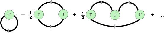
Figure 1: Diagrammatic expansion of eq. (A). Every thick line corresponds to the insertion of a Fermi-sea and each circle to the insertion of an operator $\Gamma\equiv-iA\left[I_{4}-D_{0}^{-1}A\right]^{-1}$. Notice that each of the three in-medium baryon closed loops shown in the figure is a different generalized in-medium vertex.

As sketched in appendix A and detailed in [1], each thick solid line corresponds to summing over all the plane wave states of the proton(neutron) Fermi-sea with three-momentum smaller than $k_{F}^{(p)}$($k_{F}^{(n)}$). In the following we count any Fermi momentum $k_{F}$ (about $\sim 2M_{\pi}$ for nuclear saturation density $\rho_{0}=0.17$ fm^-3) as $M_{\pi}\sim{\mathcal{O}}(p)$. Then each thick line, because of the three-momentum integration up to the Fermi momentum, is ${\mathcal{O}}(p^{3})$. Next, consider the non-local vacuum vertices $\Gamma\equiv-iA[I_{4}-D_{0}^{-1}A]^{-1}$, see fig. 2.

Figure 2: Expansion of the non-local vacuum vertex $\Gamma\equiv=-iA\left[I_{4}-D_{0}^{-1}A\right]^{-1}$, where $I_{4}$ is the $4\times 4$ unit matrix. Every solid line corresponds to a vacuum baryon propagator $iD_{0}^{-1}$ and each circle to the insertion of an operator $-iA$ from $\bar{\psi}D\psi$.

Given the pion-nucleon Lagrangian ${\cal L}_{\pi N}=\bar{\psi}D(x)\psi$, the operator $A$ is itself subject to a chiral expansion, $A=\sum_{i}A^{(i)}$, $i\geq 1$ (the terms in $A$ up to ${\mathcal{O}}(p^{2})$ are explicitly worked out in appendix B). On the other hand, a soft momentum $Q$ related to pions or external sources can be attached to each local vertex $A$. This together with the Dirac delta function of four-momentum conservation implies that the momenta running along the baryon propagators $D_{0}^{-1}$ just differ from each other by quantities of order $Q\sim{\mathcal{O}}(p)$. Since at least one Fermi-sea insertion (thick line) is required for any in-medium contribution, with on-shell four-momentum $p$, the four-momentum $p_{j}$ running along the $j^{th}$ free baryon propagator $iD_{0}^{-1}(p_{j})$, is $p_{j}=p+Q_{j}$. In this way the natural chiral power counting of such propagators can be obtained by expanding them as,

$$iD_{0}^{-1}(p_{j}) = i\frac{\not\mathrel{p}+\not\mathrel{Q}_{j}+m_{N}}{(p+Q_{j})^{2}-m_{N}^{2}+i\epsilon}=i\frac{\not\mathrel{p}+\not\mathrel{Q}_{j}+m_{N}}{Q_{j}^{2}+2Q_{j}^{0}E_{N}(p)-2{\mathbf{Q}}_{j}\mathbf{p}+i\epsilon}$$ (2.1)

$$= i\frac{\not\mathrel{p}+\not\mathrel{Q}_{j}+m_{N}}{2Q^{0}_{j}m_{N}+i\epsilon}\left(1-\frac{Q_{j}^{2}-2{\mathbf{Q}}_{j}\mathbf{p}}{2Q_{j}^{0}m_{N}}+{\mathcal{O}}(p^{2})\right)~{}.$$

Thus $iD_{0}^{-1}$ counts as ${\cal O}(p^{-1})$. As a result every $\Gamma$ vertex with $m_{\Gamma}\geq 0$ free baryon propagators and $(m_{\Gamma}+1)$ $A$ vertices (see fig. 2) scales as $p^{\nu_{\Gamma}}$ with

$$\nu_{\Gamma}=\sum_{j=1}^{m_{\Gamma}+1}d_{j}-m_{\Gamma}~{},$$ (2.2)

where $d_{j}$ is the chiral dimension of the vertex $A_{j}$. Next, we will consider the chiral counting of in-medium non-local vertices, some of them are shown in fig. 1. The chiral counting of an in-medium non-local vertex (labeled by $\rho$) that is generated through the exchange of $n\geq 1$ Fermi-sea insertions, $n$ non-local vacuum $\Gamma$ vertices, $V=n+m$ local $A$ vertices and $m=\sum_{i}m_{\Gamma_{i}}$ free baryon propagators is given by

$$d_{\rho}=3n+\sum_{i=1}^{n}\nu_{\Gamma_{i}}-4(n-1)=3n+\sum_{i=1}^{V}d_{i}-m-4(n-1)=\sum_{i=1}^{V}d_{i}-V+4=4+\sum_{i=1}^{V}(d_{i}-1)~{}.$$ (2.3)

Here the factor $4(n-1)$ originates from the four-momentum Dirac deltas attached to any $\Gamma$ vertex. Now, since $d_{i}\geq 1$, any such diagram will count at least as ${\cal O}(p^{4})$. The lowest order is obtained when only $A^{(1)}$ operators with $d_{i}=1$ are included. The next-to-leading order implies the inclusion of one $A^{(2)}$ operator and is ${\mathcal{O}}(p^{5})$.

Finally one has to take into account the exchange of pions inside or between generalized in-medium vertices or between them and pure pion vertices coming from the vacuum chiral Lagrangian ${\cal L}_{\pi\pi}$ or between the latter alone. Denoting by $I_{\pi}$ the total number of internal pion lines and by $L_{\pi}$ the numbers of pion loops, $L_{\pi}=I_{\pi}-V_{\rho}-V_{\pi}+1$ where $V_{\pi}$ is the number of vertices from ${\cal L}_{\pi\pi}$ and analogously $V_{\rho}$ is the number of generalized in-medium vertices. Hence a many-particle diagram originating from the Lagrangians ${\cal L}_{\pi\pi}$ and ${\cal L}_{\pi N}$ has the chiral power $\nu$,

$$\nu=4L_{\pi}-2I_{\pi}+\sum_{i=1}^{V_{\pi}}d_{i}+\sum_{i=1}^{V_{\rho}}d_{\rho i}=2L_{\pi}+2+\sum_{i=1}^{V_{\pi}}(d_{i}-2)+\sum_{i=1}^{V_{\rho}}(d_{\rho i}-2)=2L_{\pi}+2+\sum_{i=1}^{V_{T}}(\delta_{i}-2)$$ (2.4)

with $V_{T}=V_{\pi}+V_{\rho}$ and $\delta_{i}$ is the chiral dimension of any vertex, either from ${\cal L}_{\pi\pi}$ or from the in-medium generalized vertices. We do not differentiate between $d_{i}$ and $d_{\rho i}$ and use the symbol $\delta_{i}$ wherever no confusion can arise whether a vertex comes from the free–space Lagrangian or is an in-medium generalized one. The counting based on eq. (2.4) is from here on referred to as the standard case.

As a result the leading in-medium contribution begins at ${\cal O}(p^{4})$, since $d_{\rho}\geq 4$ from eq. (2.3) with $V_{\rho}=1$ and $L_{\pi}=0$. In this work we will calculate the next-to-leading order in-medium corrections, ${\cal O}(p^{5})$, to several $n-$point Green functions whenever the previous counting holds, see below. The ${\mathcal{O}}(p^{4})$ vacuum corrections to the leading non-vanishing ${\mathcal{O}}(p^{2})$ results can be found in ref. [3], except for the anomalous $\pi^{0}\to\gamma\gamma$ decay (which only starts at fourth order in the chiral expansion since it is an anomalous process), and when necessary we will just give the corresponding vacuum results. As it is clear from eq. (2.4), any pion loop or any extra generalized in-medium vertex increases the chiral power by at least two more orders, ${\cal O}(p^{6})$. Thus the leading $\rho-$corrections, according to eqs. (2.3), (2.4) are of order $p^{4}$ and $p^{5}$ and come from the insertion of one generalized $\rho-$vertex with only $A^{(1)}$ operators or with one additional $A^{(2)}$, respectively. We state once again that it is beyond the scope of the present work, and beyond the present knowledge, to derive a full in-medium effective field theory which includes as well nucleon-nucleon contact interactions.

2.2 Chiral counting: Non-standard case

There is one subtlety with the power counting developed so far. To understand this, we remark that the propagator of a nucleon in the heavy baryon formulation with four-momentum $p_{j}$ is $1/(Q_{j}^{0}+i\epsilon)$. This corresponds to the leading non-relativistic term of the expansion given in eq. (2.1) which was used in order to determine the dimension of $iD_{0}^{-1}(p_{j})$. One caveat, already present in vacuum, arises when the energy $Q_{j}^{0}$ is fixed and vanishes. In this case the heavy baryon propagator blows up although in a relativistic formalism used here (or in a non-relativistic one by keeping the kinetic energy) one still has $iD_{0}^{-1}(p_{j})=-i(\not\mathrel{p}+\not\mathrel{Q}_{j}+m)/({\mathbf{Q}}_{j}^{2}+2{\mathbf{Q}}_{j}{\mathbf{p}}+i\epsilon)$. The result is finite, but now $iD_{0}^{-1}(p_{j})$ counts as ${\cal O}(p^{-2})$ instead of ${\cal O}(p^{-1})$ as it was used to derive eq. (2.4). To deal with this case, it is necessary to subtract the number of baryon lines, $I_{B}^{\star}$, with $Q_{j}^{0}\lesssim k_{F}^{2}/2m_{N}$ from eq. (2.4). We can write an upper bound of this number in terms of the number of loops, vertices and external lines. To see this note that the number of pion plus external source legs is greater or equal to the number of baryon lines, which can be free propagators as well as Fermi-sea insertions. We make use of the fact that each $A$ vertex will involve at least one pion or external source, otherwise it is absorbed in the physical value of the nucleon masses, as explained in appendix B. We denote by $E_{x}$ the number of external legs and by $I_{B}$ the number of baryon lines minus $V_{\rho}$, since for every generalized vertex we have at least one Fermi-sea insertion. Then we have

$$E_{x}+2I_{\pi}-V_{\rho}\geq I_{B}~{}.$$ (2.5)

Substituting in this expression $I_{\pi}=L_{\pi}+V_{T}-1$, one obtains

$$E_{x}+2L_{\pi}+V_{\rho}+2V_{\pi}-2\geq I_{B}~{}.$$ (2.6)

We can further restrict the previous inequality by subtracting $2V_{\pi}$ on the left hand side (l.h.s.) since for each vacuum vertex there are at least two legs attached to it when calculating any in-medium contribution. Moreover, in the case of diagrams without any external source we can subtract $4V_{\pi}$ because any vacuum vertex should have at least four pion legs. Otherwise it just contributes to the vacuum renormalized pion propagators and associated wave function renormalizations, which can be calculated anyhow just from ${\cal L}_{\pi\pi}$ to the required accuracy. We will denote by a) the first case and by b) the more specific second one. Then we can write:

a) $$E_{x}+2L_{\pi}+V_{\rho}-2\geq I_{B}~{},$$ (2.7)

b) $$E_{x}+2L_{\pi}+V_{\rho}-2-2V_{\pi}\geq I_{B}~{}.$$

We now indicate by $n_{m}$ the number of $A$ vertices with $m$ attached legs. Then for each of such vertices $m-1$ lines are non-baryonic and can be removed from the l.h.s of eqs. (2.7). In the same way, we call $p_{m}$ the number of vacuum vertices from ${\cal L}_{\pi\pi}$ with $m$ legs. For the case a) we have already subtracted $-2V_{\pi}$ and for the case b) $-4V_{\pi}$. Thus we can further remove $m-2$ for a) and $m-4$ for b). Putting all this together, we arrive at the equalities:

a) $$E_{x}+2L_{\pi}+V_{\rho}-2-\sum_{m\geq 2}(m-1)n_{m}-\sum_{m\geq 3}(m-2)p_{m}=I_{B}~{},$$ (2.8)

b) $$E_{x}+2L_{\pi}+V_{\rho}-2-2V_{\pi}-\sum_{m\geq 2}(m-1)n_{m}-\sum_{m\geq 5}(m-4)p_{m}=I_{B}~{}.$$

Notice that the second of these equations is just a rewriting of the first one for the special case with only pion legs. In summary, after the elimination of $L_{\pi}$ and the subtraction of $I_{B}^{\star}$, the counting index $\nu$ given in eq. (2.4) changes to

a) $$\nu=4+\sum^{V_{\rho}}_{i=1}(\delta_{i}-3)+\sum^{V_{\pi}}_{i=1}(\delta_{i}-2)-E_{x}+\sum_{m\geq 2}(m-1)n_{m}+\sum_{m\geq 3}(m-2)p_{m}+\left(I_{B}-I_{B}^{\star}\right)~{},$$ (2.9)

b) $$\nu=4+\sum^{V_{\rho}}_{i=1}(\delta_{i}-3)+\sum^{V_{\pi}}_{i=1}\delta_{i}-E_{x}+\sum_{m\geq 2}(m-1)n_{m}+\sum_{m\geq 5}(m-4)p_{m}+\left(I_{B}-I_{B}^{\star}\right)~{}.$$

When $V_{\pi}=0$, we adopt the convention that there is no contribution from the second and fourth sums on the right hand side (r.h.s) of the last equation. The interesting point of these equations is that for a given number of external legs $E_{x}$ the chiral dimension $\nu$ is bounded since $\delta_{i}\geq 4$ for a generalized in-medium vertex as shown above and $\delta_{i}\geq 2$ for any vertex from ${\cal L}_{\pi\pi}$ and by definition $I_{B}\geq I_{B}^{\star}$. Note also that the inclusion of an extra generalized $\rho-$vertex increases $\nu$ at least by 1. Those loops that arise because of pion lines that are exchanged inside only one generalized $\rho-$vertex will increase $I_{B}-I_{B}^{\star}$ by the number of involved baryon propagators in the loops because of the absence of the so called pinch singularity [18]. However, when two or more $\rho-$vertices are involved in the pion loops this is no longer the case. We will apply these counting rules when discussing in-medium pion condensation and $4\pi$ scattering. In the latter case, we will just calculate the leading contribution ${\mathcal{O}}(p^{3})$. The counting based on eq. (2.9) is from here on referred to as the non-standard case.

In the sections 3–5, we will use the simpler counting rules, see eq. (2.4), to determine the diagrams to be considered up to ${\mathcal{O}}(p^{5})$, with the exception of those cases cases where a small energy denominator occurs, $Q_{j}^{0}\simeq k_{F}^{2}/2m_{N}$, and where we will turn to eq. (2.9). This will always be indicated in the text at the appropriate places.

Finally, let us stress again the difference in the power counting for pion properties in the medium and in the vacuum. While in vacuum the leading and next-to-leading order is ${\cal O}(p^{2})$ and ${\cal O}(p^{4})$, respectively, in the medium and for the standard case, these contributions start at ${\cal O}(p^{4})$ and ${\cal O}(p^{5})$, respectively.

3 In-medium quark condensates

From the generating functional ${\cal Z}(v,a,s,p)$ given in eq. (A), the quark condensate is obtained by partial functional differentiation,

$$\langle\Omega|\bar{q}_{i}q_{j}|\Omega\rangle=-\frac{\delta}{\delta s_{ij}(x)}{\cal Z}(v,a,s,p)\arrowvert_{v,a,s,p=0}~{},$$ (3.1)

with $q_{1}=u$ and $q_{2}=d$ quarks. Up to ${\cal O}(p^{5})$, because of the absence of pion loops, the in-medium contributions can be calculated directly by equating the generating functional ${\cal Z}$ with the in-medium action $\int dx\widetilde{\cal L}_{\pi\pi}(x)$ and the vertex can be identified by doing the partial derivative $\frac{\partial}{\partial s_{ij}(x)}A^{(2)}(x)$. The resulting $\rho-$diagram is depicted in fig. 3 with one insertion from $A^{(2)}$, since the scalar source $s(x)$ is not present in $A^{(1)}$ (see eqs. (B.5) and (B.6)).

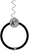
Figure 3: Unique diagram that contributes to the calculation of the in-medium quark condensates up to ${\mathcal{O}}(p^{5})$. As usual the thick line represents a Fermi-sea insertion, the circle is an $A^{(2)}$ vertex and the wavy line an external scalar source $s(x)$.

We denote by $\rho_{p}$ and $\rho_{n}$ the proton and neutron densities, in order. These are given by

$$\rho_{p}=2\int^{k_{F}^{(p)}}\!\!\!\frac{d\mathbf{p}}{(2\pi)^{3}}=\frac{(k_{F}^{(p)})^{3}}{3\pi^{2}}~{},\qquad\rho_{n}=2\int^{k_{F}^{(n)}}\!\!\!\frac{d\mathbf{p}}{(2\pi)^{3}}=\frac{(k_{F}^{(n)})^{3}}{3\pi^{2}}~{},$$ (3.2)

and we also introduce the quantities $\hat{\rho}=(\rho_{p}+\rho_{n})/2$, the isospin symmetric nuclear density, and $\bar{\rho}=(\rho_{p}-\rho_{n})/2$, the isospin asymmetric nuclear density. It is easy to see from eqs. (A) and (B.6) that the in-medium contributions to the action $\int dx\,\widetilde{{\cal L}}$ which contain the scalar sources (the ones relevant for the calculation of the quark condensates) are:

$$\int dx\int\frac{d{\mathbf{p}}}{(2\pi)^{3}2E(p)}\hbox{Tr}\Bigl{[}\left\{c_{1}4B_{0}\langle s(x)\rangle+c_{5}\left[4B_{0}s(x)-2B_{0}\langle s(x)\rangle\right]\right\}n(p)(\not\mathrel{p}+m_{N})\Bigr{]}$$

$$=\int dx\Bigl{[}4B_{0}\hat{\rho}(2c_{1}-c_{5})(s_{11}(x)+s_{22}(x))+4B_{0}c_{5}(s_{11}(x)\rho_{p}+s_{22}(x)\rho_{n})\Bigr{]}+{\mathcal{O}}(p^{6})~{},$$ (3.3)

where the usual SU(2) matrix notation is applied for the scalar source. By differentiating with respect to $s_{11}(x)$ and $s_{22}(x)$ one obtains, respectively, the up- and the down-quark condensates at ${\mathcal{O}}(p^{5})$:

$$\langle\Omega|\bar{u}u|\Omega\rangle = \langle\bar{u}u\rangle_{\rm vac}\left[1-\frac{2\sigma}{f^{2}M_{\pi}^{2}}\hat{\rho}+\frac{4c_{5}}{f^{2}}\bar{\rho}\right]~{},$$

$$\langle\Omega|\bar{d}d|\Omega\rangle = \langle\bar{d}d\rangle_{\rm vac}\left[1-\frac{2\sigma}{f^{2}M_{\pi}^{2}}\hat{\rho}-\frac{4c_{5}}{f^{2}}\bar{\rho}\right]~{},$$ (3.4)

with the pion-nucleon sigma-term $\sigma=-4c_{1}M_{\pi}^{2}$ at ${\mathcal{O}}(p^{2})$ [22, 23]. Furthermore, the subscript $\rm vac$ refers to the vacuum value of the corresponding quantity up to ${\mathcal{O}}(p^{4})$ as given in ref. [3], which at lowest order is simply $-B_{0}f^{2}$.

Keeping terms up to the same accuracy, the isoscalar sum $\langle\Omega|\bar{u}u+\bar{d}d|\Omega\rangle=\langle\bar{u}u+\bar{d}d\rangle_{\rm vac}\left[1-2\sigma\hat{\rho}/f^{2}M_{\pi}^{2}\right]$ only depends on the total nuclear density $2\hat{\rho}=\rho_{p}+\rho_{n}$ and agrees with the expression, valid up to linear order in the density, given in ref. [24] under the use of the Hellmann-Feynman theorem (we are using a chiral perturbative approach and the agreement is only valid strictly when calculating the $\sigma$-term up to ${\mathcal{O}}(p^{2})$ as noted above). For a more intuitive derivation, see ref. [25]. This coincidence is not surprising since, in the non-relativistic limit, the diagram of fig. 3 just counts the number of nucleon states times the corresponding vertex for protons and neutrons separately. If one assumes an expansion in density on intuitive grounds this has to be the leading result. This is indeed the argument used in ref. [25]. Note that deviations from the relativistic limit in fig. 3 increase the counting by two orders. As a new aspect with respect to previous works [25, 24, 12] we also consider strong isospin breaking represented by the term with $c_{5}$ in eq. (3). Other works that also consider the calculation of the quark condensates in symmetric nuclear matter are refs. [12, 11] within a mean-field approach and refs. [26, 27, 28, 29] using the Nambu-Jona-Lasinio model. Note also that the quark condensates are essential inputs of in-medium QCD sum rules techniques [30, 25].

For the case of symmetric nuclear matter, all the previous investigations led to dropping quark condensates with increasing density. Specifically, using the value for the $\sigma$–term, $\sigma=44\pm 8\pm 7$ MeV [31], one obtains a relative reduction of a $(35\pm 9)\%$ with respect to its vacuum value for nuclear matter density. This reduction of the quark condensate with density is traditionally considered as a clear indication of chiral symmetry restoration in the nuclear medium [26]. At this point it is worthwhile to stress that the quark condensate is not a unique order parameter of chiral symmetry breaking. Even if it vanishes, chiral symmetry is still spontaneously broken as long as $f^{2}\neq 0$. We will come back to this point below when evaluating the in-medium weak decay couplings of the pion. We also note from eq. (3) that the correction becomes unity when $\rho\sim 2.8\rho_{0}$ corresponding to a Fermi-momentum $k_{F}\sim 400$ MeV. However, this value should also be considered indicative since then the correction is equal to the leading term.

Consider now the isospin breaking contribution. From ref. [23] we take the value $c_{5}=-0.09\pm 0.01$ GeV^-1. For realistic cases $\rho_{n}\geq\rho_{p}$ and then since $c_{5}<0$, the in-medium $\bar{d}d$ condensate is smaller than the $\bar{u}u$ one. Using $\langle\bar{u}u\rangle_{\rm vac}=\langle\bar{d}d\rangle_{\rm vac}=\frac{1}{2}\langle\bar{q}q\rangle_{\rm vac}$ in the limit $m_{u}=m_{d}$ [3], the pertinent difference is:

$$\langle\Omega|\bar{u}u-\bar{d}d|\Omega\rangle=\langle\bar{q}q\rangle_{\rm vac}\frac{4\,c_{5}}{f^{2}}\bar{\rho}\simeq\langle\bar{q}q\rangle_{\rm vac}\,\,0.028\,\frac{\rho_{n}-\rho_{p}}{\rho_{0}},$$ (3.5)

which is very suppressed as compared to the density dependence of the sum given by

$$\langle\Omega|\bar{u}u+\bar{d}d|\Omega\rangle\simeq\langle\bar{q}q\rangle_{\rm vac}\left[1-0.35\frac{\rho_{n}+\rho_{p}}{\rho_{0}}\right]~{},$$ (3.6)

because $-2c_{5}$, see. eq. (3), is more than one order of magnitude smaller than $\sigma/M_{\pi}^{2}\sim 2.3$ GeV^-1. Hence the presence of the terms in eq. (3) proportional to $c_{5}$ does not alter appreciably the reduction of the quark condensates at finite density present in the symmetric nuclear matter case studied in refs. [26, 24, 12].

4 Two-point Green functions

We now consider the propagation of pions in the medium. We will first derive their equations of motion from which one can read off the in-medium pion mass. We will also discuss pion-condensation illustrating the use of eq. (2.9). In addition the new scales for the in-medium chiral expansion are also pointed out. The $\rho-$wave function renormalization of pions needed to satisfy the quantum canonical commutation relations is derived in appendix D. Finally, we will also study the couplings of pions to the axial-vector and pseudoscalar currents in the medium and their relation as dictated by a QCD Ward identity.

4.1 Equations of motion

In fig. 4 we show those diagrams that give the in-medium corrections of the pion propagator up to ${\mathcal{O}}(p^{5})$. As pointed out in ref. [1], the $\rho-$vertices have analogous properties to those of the standard local vertices (i.e. the field theoretical vertices from ${\cal L}_{\pi\pi}$) in the computation of the numerical factors accompanying the exchange of pion lines in a given diagram. With respect to fig. 4 this manifests itself in the fact that together with the momentum $Q$ flowing from the left to the right, as in particular shown in fig. 4b, one has also to consider the inverse process, $Q\rightarrow-Q$. This is immediately accomplished when working in configuration space.

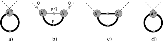
Figure 4: Diagrams that contribute to the in-medium propagation of pions up to ${\mathcal{O}}(p^{5})$. Figs.a), b) and c) are ${\mathcal{O}}(p^{4})$ and fig.d) is ${\mathcal{O}}(p^{5})$. The crossed diagram of b), obtained by replacing $Q\rightarrow-Q$, is not shown. The energy through the pion lines (dashed) is $\sim M_{\pi}$.

Denoting by $Q$ the pion four-momentum and by $p$ the one running in the (lower) Fermi-sea insertion ($p^{2}=m_{N}^{2}$) in each diagram of fig. 4, one can easily see that the imaginary parts of the diagrams in this figure vanish for $Q^{0}\sim M_{\pi}\gg Q^{2}/(2m_{N})$. Note that the presence of the pole of the baryon propagating with four-momentum $p-Q$ in fig. 4 implies the vanishing of the denominator $(p-Q)^{2}-m_{N}^{2}=Q^{2}-2pQ$. This occurs only when $Q^{0}\simeq Q^{2}/2m_{N}$ which is not the case for $Q^{2}\sim M^{2}_{\pi}$, i.e. for the type of pion momenta considered in most parts of this work. The same reasoning can be applied to fig. 4c. Denoting by $q$ the four-momentum of the second Fermi-sea insertion we then have $(p-Q)^{2}=q^{2}=m_{N}^{2}$ which is once again the same equation as the one required to pick the pole in fig. 4b. In fact, the imaginary parts of fig. 4b and fig. 4c are closely linked and tend to cancel each other. Remembering the Feynman rules of appendix A, a second Fermi-sea insertion implies an extra factor of

$$-\frac{1}{2}\int^{k_{F}}\!\!\frac{d{\mathbf{q}}}{(2\pi)^{3}2E(q)}(\not\mathrel{q}+m_{N}),$$ (4.1)

as compared to the case with only one Fermi-sea insertion. On the other hand, putting a baryon on-shell in fig. 4b implies

$$i\int\frac{dq}{(2\pi)^{4}}\frac{\not\mathrel{q}+m_{N}}{q^{2}-m_{N}^{2}+i\epsilon}\rightarrow\frac{1}{2}\int\frac{d{\mathbf{q}}}{(2\pi)^{3}\,2E(q)}\left[(\not\mathrel{q}+m_{N})-(\tilde{\not\mathrel{q}}-m_{N})\right]~{},$$ (4.2)

with the four-momentum $\tilde{q}=(E(q),-{\bf{q}})$. The second term on the r.h.s. of this equation comes from the anti-baryon pole and does not contribute because of the presence of an extra delta function $\delta(q^{0}-p^{0}-Q^{0}_{j})$ which cannot be satisfied since in this case $q^{0}=-E(q)$ and $p^{0}$ is an on-shell baryon momentum coming from the sum over the states in the Fermi-sea as already discussed. Then only the first term on the r.h.s. of eq. (4.2) is possible and by splitting the three-momentum integral as $\int^{\infty}d{\bf{q}}=\int^{k_{F}}d{\bf{q}}+\int_{k_{F}}^{\infty}d{\bf{q}}$, we see that the integration up to $k_{F}$ cancels against eq. (4.1), leaving only $\int_{k_{F}}^{\infty}d{\bf{q}}$. This implies that the absorptive parts, arising by exciting one baryon on-shell, begin to contribute only when the baryon-three-momentum is larger than $k_{F}$ (particle excitation), as one could naturally expect since all the other states in the Fermi-sea are already occupied.

Introducing the density matrix $\rho={\rm diag}(\rho_{p},\rho_{n})$, the in-medium contributions to the quadratic pionic term of $\widetilde{{\cal L}}$, $\delta\widetilde{{\cal L}}_{\phi\phi}$, can be obtained from eq. (A) (as just discussed, the last term of eq. (A) with two Fermi-sea insertions does not contribute here). We then obtain

$$i\int dx\delta\tilde{{\cal L}}_{\phi\phi}(x) = -\frac{1}{8f^{2}}\int dx\langle\rho[\phi,\dot{\phi}]\rangle+\frac{i}{f^{2}}\int dx\Big{\langle}\rho\bigg{\{}-2c_{1}B_{0}\langle\phi^{2}{\cal M}\rangle+\frac{1}{2}c_{2}\langle\dot{\phi}\dot{\phi}\rangle+\frac{1}{2}c_{3}\langle\partial_{\mu}\phi\partial^{\mu}\phi\rangle$$

$$- \frac{1}{2}c_{5}B_{0}\left(\phi^{2}{\cal M}+{\cal M}\phi^{2}+2\phi{\cal M}\phi\right)+c_{5}B_{0}\langle\phi^{2}{\cal M}\rangle\bigg{\}}\Big{\rangle}$$

$$- \frac{ig_{A}^{2}}{4f^{2}}\int\frac{d\mathbf{p}}{(2\pi)^{3}2E(p)}\int dxdy\,e^{ip(x-y)}\hbox{Tr}\bigg{\{}\gamma^{\mu}\gamma_{5}\partial_{\mu}\phi(x)D_{0}^{-1}(x,y)\gamma^{\nu}\gamma_{5}\partial_{\nu}\phi(y)(\not\mathrel{p}+m_{N})n(p)\bigg{\}},$$

where the Cartesian coordinates for the pion fields are defined by $\phi=\sum_{i=1}^{3}\phi_{i}\tau_{i}$ with $\phi$ given in eq. (B.4) and $\tau_{i}$ are the usual Pauli matrices. In the last expression we have set $\stackrel{{\scriptstyle\circ}}{{g}}_{A}$ to its physical value $g_{A}=1.267$ since corrections will be of higher orders than the next-to-leading one, $g_{A}=\stackrel{{\scriptstyle\circ}}{{g}}_{A}\{1+{\cal O}(\hat{m})\}$[32], and for the same reason we take in the following $m_{p}=m_{n}=m_{N}=(m_{n}+m_{p})/2\simeq 939\hbox{ MeV}$ as mentioned in appendix A.

The in-medium contribution to the equations of motion are obtained by performing the differentiation $\delta\int dy\widetilde{{\cal L}}_{\phi\phi}/\delta\phi_{k}(x)$. Working in momentum-space, $\phi_{k}(x)=\int\frac{dQ}{(2\pi)^{4}}\,e^{-iQx}\phi_{k}(Q)$, one obtains:

$$- \frac{g_{A}^{2}\hat{\rho}}{2f^{2}m_{N}}\frac{(Q^{2})^{2}}{Q_{0}^{2}}\phi(Q)_{k}-i\frac{g_{A}^{2}\bar{\rho}}{f^{2}}\left(Q_{0}-\frac{Q^{2}}{Q_{0}}\right)\epsilon_{kj3}\phi(Q)_{j}+i\frac{\bar{\rho}}{f^{2}}Q_{0}\epsilon_{kj3}\phi(Q)_{j}-\frac{16B_{0}}{f^{2}}\hat{\rho}\hat{m}c_{1}\phi(Q)_{k}$$ (4.4)

$$+ \frac{4\hat{\rho}}{f^{2}}\left(c_{2}Q_{0}^{2}+c_{3}Q^{2}\right)\phi(Q)_{k}-\frac{8B_{0}}{f^{2}}\bar{\rho}\bar{m}c_{5}\delta_{3k}\phi(Q)_{3}~{}.$$

Diagonalizing these equations by working in terms of the charged fields $\pi^{+}=(\phi_{1}-i\phi_{2})/\sqrt{2}$ and $\pi^{-}=(\phi_{1}+i\phi_{2})/\sqrt{2}$, together with $\pi^{0}=\phi_{3}$ and adding the vacuum piece, we finally have the following spectral relations between the energy $Q_{0}\equiv\omega$ and the three-momentum $\mathbf{Q}$ for on-shell in-medium pions:

$$\mathbf{\pi^{0}:}$$

$$\omega^{2}-M_{\pi^{0}}^{2}\left(1+c_{1}\frac{8\hat{\rho}}{f^{2}}\right)+\frac{4\hat{\rho}}{f^{2}}\omega^{2}\left(c_{2}+c_{3}-\frac{g_{A}^{2}}{8m_{N}}\right)-{\mathbf{Q}^{2}}\left(1+\frac{4\hat{\rho}}{f^{2}}c_{3}-\frac{g_{A}^{2}\hat{\rho}}{m_{N}f^{2}}\right)-\frac{g_{A}^{2}\hat{\rho}}{2f^{2}m_{N}}\frac{({\mathbf{Q}}^{2})^{2}}{\omega^{2}}$$

$$-\hat{M}_{\pi}^{2}\frac{4\bar{\rho}}{f^{2}}\frac{\bar{m}}{\hat{m}}c_{5}=0~{},$$

$$\mathbf{\pi^{+}:}$$

$$\omega^{2}-M_{\pi^{+}}^{2}\left(1+c_{1}\frac{8\hat{\rho}}{f^{2}}\right)+\frac{4\hat{\rho}}{f^{2}}\omega^{2}\left(c_{2}+c_{3}-\frac{g_{A}^{2}}{8m_{N}}\right)-{\mathbf{Q}}^{2}\left(1+\frac{4\hat{\rho}}{f^{2}}c_{3}-\frac{g_{A}^{2}\hat{\rho}}{m_{N}f^{2}}\right)-\frac{g_{A}^{2}\hat{\rho}}{2f^{2}m_{N}}\frac{({\mathbf{Q}}^{2})^{2}}{\omega^{2}}$$

$$+\frac{g_{A}^{2}\bar{\rho}}{f^{2}\omega}{\mathbf{Q}}^{2}-\frac{\bar{\rho}\omega}{f^{2}}=0~{},$$

$$\mathbf{\pi^{-}:}$$ (4.5)

$$\omega^{2}-M_{\pi^{+}}^{2}\left(1+c_{1}\frac{8\hat{\rho}}{f^{2}}\right)+\frac{4\hat{\rho}}{f^{2}}\omega^{2}\left(c_{2}+c_{3}-\frac{g_{A}^{2}}{8m_{N}}\right)-{\mathbf{Q}}^{2}\left(1+\frac{4\hat{\rho}}{f^{2}}c_{3}-\frac{g_{A}^{2}\hat{\rho}}{m_{N}f^{2}}\right)-\frac{g_{A}^{2}\hat{\rho}}{2f^{2}m_{N}}\frac{({\mathbf{Q}}^{2})^{2}}{\omega^{2}}$$

$$-\frac{g_{A}^{2}\bar{\rho}}{f^{2}\omega}{\mathbf{Q}}^{2}+\frac{\bar{\rho}\omega}{f^{2}}=0~{},$$

with $\hat{M}_{\pi}^{2}=2\hat{m}B_{0}$ the lowest order CHPT pion masses and $M_{\pi^{0}}$, $M_{\pi^{+}}$ the vacuum pion masses at ${\mathcal{O}}(p^{4})$[3]. We will take all of them to coincide with the corresponding physical masses since differences will be ${\mathcal{O}}(p^{6})$.

4.2 Pion dispersion and condensation

The previous expressions largely simplify in the case of symmetric nuclear matter $\bar{\rho}=0$ in the chiral limit,

$$\omega^{2}={\mathbf{Q}}^{2}\left(1-\frac{4\hat{\rho}}{f^{2}}c_{2}\right).$$ (4.6)

The pion velocity in-medium for this case is given by:

$$\widetilde{v}=\frac{d\omega}{d|\mathbf{Q}|}=1-\frac{2\hat{\rho}}{f^{2}}c_{2}.$$ (4.7)

Since it must be smaller than the velocity of light [17, 33], this imposes the constraint $c_{2}\geq 0$ which is satisfied by the actual value of this constant, $c_{2}=3.2\pm 0.25$ GeV^-1[34]. Imposing $\widetilde{v}\geq 0$, then $c_{2}\leq f^{2}/2\hat{\rho}$. Taking the previous value for $c_{2}$ gives $\rho\leq 2\rho_{0}$. This clearly indicates that in-medium CHPT, just by considering $\pi N$ interactions with the actual values of the $c_{i}$ counterterms, can only be applied to densities $\lesssim\rho_{0}$, as otherwise the corrections will be larger than $50\%$. For $\rho_{0}$ (nuclear matter saturation density), $k_{F}\simeq 270\,$MeV$\sim 2M_{\pi}$. Even for vacuum $\pi N$ scattering, such a value for the running three-momentum is on edge of applicability of the theory [34, 35]. However, one also has to take into account that due to the large variation in the values of the $c_{i}$ and combinations of them, important differences with respect to the actual scale for a specific process are expected; see section 4.3 for a discussion about the scales at which the chiral expansion breaks down.

We are now interested in finding solutions to eqs. (4.1) with vanishing energy so that the ground state becomes unstable against the spontaneous creation of pion modes. A close look to eqs. (4.1) indicates the presence of possible solutions in the antisymmetric matter case, with ${\mathbf{Q}}^{2}/\omega={\rm constant}$ for $\omega,{\mathbf{Q}}\rightarrow 0$. To be more specific, let us consider eq. (4.1) for negative pions $\pi^{-}$. Then for $\omega,{\mathbf{Q}}\rightarrow 0$ and ${\mathbf{Q}}^{2}/\omega=D$ one has the equation:

$$\frac{g_{A}^{2}\hat{\rho}}{2f^{2}m_{N}}D^{2}+\frac{g_{A}^{2}\bar{\rho}}{f^{2}}D+M^{2}_{\pi^{+}}\left(1+\frac{8c_{1}\hat{\rho}}{f^{2}}\right)=0$$ (4.8)

with the solution:

$$D=\frac{f^{2}m_{N}}{g_{A}^{2}\hat{\rho}}\left[-\frac{g_{A}^{2}\bar{\rho}}{f^{2}}\pm\sqrt{\left(\frac{g_{A}^{2}\bar{\rho}}{f^{2}}\right)^{2}-\frac{2g_{A}^{2}\hat{\rho}}{f^{2}m_{N}}M_{\pi^{+}}^{2}\left(1+\frac{8c_{1}\hat{\rho}}{f^{2}}\right)}\,\right].$$ (4.9)

In order to have an oscillatory mode and not a diffuse one, the following inequality has to be fulfilled,

$$\rho\geq\frac{4f^{2}}{g_{A}^{2}m_{N}}\left(\frac{\hat{\rho}}{\bar{\rho}}\right)^{2}M_{\pi^{+}}^{2}\left(1+\frac{8c_{1}\hat{\rho}}{f^{2}}\right).$$ (4.10)

When the previous equality holds, $D=-m_{N}\,\bar{\rho}/\hat{\rho}$. This implies that for the $\pi^{+}$, where $D=m_{N}\,\bar{\rho}/\hat{\rho}$, the energy is negative so that it is energetically favorable to excite $\pi^{+}$ modes, i.e. we have a $\pi^{+}$ boson condensate. Because of this condensate, the U(1) flavor symmetry, which is still present in eq. (A), is spontaneously broken, leading to one Goldstone boson and two heavy modes because we started with three independent pion modes. See ref. [45] for a similar discussion in the case of QCD at finite isospin density $\mu_{I}$ in the idealized case of $\mu_{B}=0$. Note also that for the neutral pion there is no such solution.

For $|\bar{\rho}|\ll\hat{\rho}$, it is justified to use eqs. (4.1) because the expansion of the baryon propagators in eq. (2.1) still holds since then $D\ll 2m_{N}$. However, when $|\bar{\rho}|\sim\hat{\rho}$ the remarks discussed at the end of sec. 2.1 apply and a more careful treatment is necessary. Still, the prior situation is approximately realized in heavy nuclei, where for $N/Z=1.5$ one has $\bar{\rho}/\hat{\rho}=-1/5$. Thus we can apply eq. (4.10) with the result:

$$\rho\geq\frac{100f^{2}}{g_{A}^{2}m_{N}}M_{\pi^{+}}^{2}\left(1+\frac{4c_{1}\rho}{f^{2}}\right)\simeq 8\rho_{0}\left(1+\frac{4c_{1}\rho}{f^{2}}\right),$$ (4.11)

so that:

$$\rho\left(1-\frac{32c_{1}\rho_{0}}{f^{2}}\right)\geq 8\rho_{0}.$$ (4.12)

The previous inequality implies:

$$\rho\geq(1.6\pm 0.2)\rho_{0}~{},$$ (4.13)

where we have used $c_{1}=-\left(0.81\pm 0.12\right)$ GeV^-1 [39]. The resulting lower limit for the density in eq. (4.13) is larger than the total density in heavy nuclei, $\rho\simeq\rho_{0}$. Therefore, these oscillatory pion modes in heavy nuclei do not occur.

For neutron star matter, $\bar{\rho}=-\hat{\rho}$, there is a reduction by a factor of 25 on the l.h.s. of eq. (4.11) so that:

$$\rho\geq\frac{4f^{2}}{g_{A}^{2}m_{N}}M_{\pi^{+}}^{2}\left(1+\frac{4c_{1}\rho}{f^{2}}\right)\simeq 0.4\rho_{0}\left(1+\frac{4c_{1}\rho}{f^{2}}\right),$$ (4.14)

which amounts to a drastic change. In fact, for this case, eq. (2.1) cannot be applied and one has to take care of the modification of the counting by making use of eq. (2.9) case b) since here we have only pion lines.

In appendix C we discuss in detail the use of the non-standard counting rules applied to the problem of the pion propagation in the medium. These results will be used in the next section when determining the appropriate in-medium scale in our framework.

4.3 In-medium breakdown scales

In this section, we will deduce the in-medium scales at which the chiral expansion breaks down. To do so let us consider eq. (A) for the generating functional or better its more general, non-perturbative expression given in ref. [1]. There, the in-medium contribution to the chiral Lagrangian is given by:

$$\int d{\mathbf{x}}\,d{\mathbf{y}}\int^{k_{F}}\!\!\frac{d{\mathbf{p}}}{(2\pi)^{3}2E(p)}e^{-i{\mathbf{p}}({\mathbf{x}}-{\mathbf{y}})}\hbox{Tr}\left\{(\not\mathrel{p}+m_{N})\log{\cal F}\right\}~{},$$ (4.15)

with $\log{\cal F}$ being a pure interaction operator whose perturbative expansion leads to eq. (A) (for definitions, see ref. [1]). In the limit $k_{F}\rightarrow 0$, the leading non-relativistic contribution, if not vanishing, comes from $\not\mathrel{p}+m_{N}\rightarrow 2\,m_{N}$ and the above expression can be written as

$$\int d{\mathbf{x}}\,d{\mathbf{y}}\hbox{Tr}\left\{2m_{N}\,\log{\cal F}\right\}\int^{k_{F}}\!\!\frac{d{\mathbf{p}}}{(2\pi)^{3}2m_{N}}=\int d{\mathbf{x}}\frac{k_{F}^{3}}{6\pi^{2}}\left(\int d{\mathbf{y}}\hbox{Tr}\left\{\log{\cal F}\right\}\right),$$ (4.16)

involving the numerical factor $1/6\pi^{2}$ and establishing that the in-medium corrections must start at order $k_{F}^{3}\propto\rho$. Taking into account the perturbative expansion of $\log{\cal F}$, given in eq. (A) [1] and noting that the local operators $A$ have dimension of mass, see e.g. eqs. (B.5) and (B.6), one concludes that any term arising from eq. (4.16) with $m$ pion fields and $n$ momenta, $n\geq 1$, counts as:

$$\frac{k_{F}^{3}}{6\pi^{2}}\frac{\phi^{m}}{f^{m}}\frac{Q^{n}}{\Lambda^{n-1}},$$ (4.17)

with $Q^{n}$ involving both derivatives and quark mass insertions and $\Lambda$ refers to a typical hadronic mass $\sim 1$ GeV. On the other hand from ${\cal L}_{\pi\pi}$ one typically has, $n\geq 2$:

$$\frac{\phi^{m}}{f^{m-2}}\frac{Q^{n}}{\Lambda^{n-2}}.$$ (4.18)

To compare eqs. (4.17) and (4.18) it is convenient to rewrite the former as:

$$\frac{k_{F}^{2}}{6\pi^{2}f^{2}}\frac{\phi^{m}}{f^{m-2}}\frac{Q^{n}k_{F}}{\Lambda^{n-1}}.$$ (4.19)

Since in our counting $k_{F}\sim Q$ we should consider $n\rightarrow n-1$, $n\geq 2$, in eq. (4.19) so that the local in-medium contributions are suppressed by $k_{F}^{2}/(6\pi f^{2})$ as compared to the vacuum ones. It is also worthwhile to stress that while the leading in-medium contribution scales as $k_{F}^{3}\sim\rho$ when $k_{F}\rightarrow 0$, eq. (4.16), the suppression with respect to a large scale surviving in the chiral limit, much larger than pion mass or momenta, involves the second and not the third order in $k_{F}$, i.e. the suppression is non-analytic in the nuclear density. Note that this scale, $\sqrt{6}f\simeq 700\,{\rm MeV}$, can also be inferred from the S-wave Weinberg-Tomozawa contribution (the last term in eqs.(4.1) for the charged pions). Under $P$-wave interaction, see the last but one term in eqs. (4.1) for the charged pions, the scale is reduced to $\sqrt{6}f/g_{A}\simeq 570\,{\rm MeV}$, a little bit larger than twice the Fermi momentum for nuclear matter saturation density. It is roughly a factor of two smaller than the commonly used value $4\pi f_{\pi}$ typically quoted in vacuum CHPT for the pion sector. This is similar to the flavor dependence $\sim 1/{N_{f}}$ pointed out in the context of extended technicolor approaches to electroweak symmetry breaking [36].

The main problem when $Q_{j}^{0}\sim Q^{2}/2m_{N}$, i.e. the non-standard scenario for the counting rules, comes from the further reduction in the scale $\Lambda$ of the nuclear perturbative expansion pertinent to such cases. In fact, instead of having the factor $2m_{N}Q^{0}$ as in eq. (2.1), one needs to consider the full expression since $Q^{0}$ counts now as a quantity of order $k_{F}^{2}/2m_{N}$ in the denominator, $k_{F}\sim{\mathcal{O}}(p)$. As a consequence, if something counted before as $k_{F}^{2}/\Lambda^{2}$, it now scales as $2m_{N}k_{F}/\Lambda^{2}$. This implies that $\Lambda\rightarrow\Lambda^{2}/2m_{N}\simeq 170$ MeV instead of $\Lambda\simeq 570$ MeV, that is, a reduction by roughly a factor of three. For instance, considering eq. (C) for the propagation of pions in the case of $\omega=0$ we have from fig. 5a, which in fact corresponds to figs.4b,c:

$$\frac{2m_{N}g_{A}^{2}{\mathbf{Q}}^{2}}{f_{\pi}^{2}}\left[\frac{k_{F}}{8\pi^{2}}+\frac{4k_{F}^{2}-{\mathbf{Q}}^{2}}{32\pi^{2}|\mathbf{Q}|}\log\frac{2k_{F}+|\mathbf{Q}|}{|2k_{F}-|\mathbf{Q}||}\right]~{}.$$ (4.20)

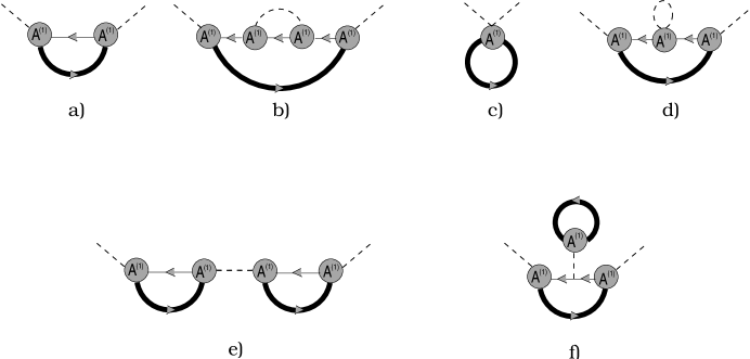
Figure 5: Diagrams that contribute to the in-medium propagation of pions up to ${\mathcal{O}}(p^{4})$ when $Q^{0}\sim k_{F}^{2}/2m_{N}$, eq. (2.9) case b). Diagram a) is ${\mathcal{O}}(p^{3})$ and the rest are ${\mathcal{O}}(p^{4})$. Other diagrams obtained by exchanging free baryon propagators by Fermi-sea insertions or by exchanging lines and or the position of loops are not shown.

Taking now $|{\bf{Q}}|\ll k_{F}$, the previous expression reduces to:

$${\bf Q}^{2}\frac{m_{N}g_{A}^{2}k_{F}}{2\pi^{2}f_{\pi}^{2}}~{},$$ (4.21)

with the scale $\Lambda^{\prime}=4\pi^{2}f_{\pi}^{2}/2m_{N}g_{A}^{2}\sim 120~{}\hbox{MeV}$, of the size we have estimated just above. As a result, while for the standard counting scenario one has a chiral expansion to be applied when $k_{F}\lesssim 2M_{\pi}$, corresponding to nuclear saturation density, when $Q_{j}^{0}\sim Q^{2}/2m_{N}$ the perturbative expansion can only be applied up to densities around $\sim\left(170~{}\hbox{MeV}/k_{F}^{0}\right)^{3}\simeq\rho_{0}/4$, where $k_{F}^{0}\simeq 268$ MeV is the Fermi momentum at nuclear matter saturation density. This modification of the scale is simply lost in the mean-field approaches to nuclear matter. However, as we have seen in sec. 4.2 and appendix C, this scale is crucial for the study of pion condensation.

For the case of the $K^{-}$ condensation in nuclear matter studied in [10] under the use of the mean-field approach, the absence of baryons with strangeness $+1$ implies that an analogous diagram to that of fig. 5a is not involved.

The previous problem is similar to that of studying nucleon-nucleon interactions in the vacuum where one also has this situation [18] due to the appearance of the large $2m_{N}\sim{\cal O}(1)$ factor instead of an ${\mathcal{O}}(p)$ one. The solution advocated in this case is to perform a resummation of diagrams by solving the Lippmann-Schwinger equation [18] and resumming those diagrams with two nucleons intermediate states. It is clear that one should proceed in a similar way here by resumming an infinite subset of diagrams, including as well nucleon contact interactions, as, on the other hand, is known for a long time in many-body problems [43, 44]. More specifically, including extra $\rho-$vertices repeatedly iterated as in fig. 5e, with any of them enhanced by the appearance of the large factor $2m_{N}/Q$, amounts to the RPA approximation for the in-medium pion propagator.

4.4 In-medium pion mass

There has been recent interest in calculating the pion masses in the medium using heavy baryon chiral perturbation theory (HBCHPT) [8, 9]. Both works include one pion loop graphs, ${\mathcal{O}}(p^{6})$, and while ref. [8] is restricted to the nuclear symmetric case, ref. [9] also considered non-symmetric nuclear matter although, as shown below, not all the effects of order ${\mathcal{O}}(p^{6})$ are included. However, the subject has already a long history and similar diagrams than those calculated in refs. [8, 9] were already considered in earlier (chiral) models [37], and the pole position of the pion propagator in nuclear matter has been discussed in the context of pion or kaon condensation, see e.g. [38]. The calculation of the in-medium pion mass implies to impose in eqs. (4.1) the condition $\bf{Q}=0$ and then to solve for $\omega=\widetilde{M}_{\pi}$, where the tilde denotes in-medium pion mass (afterwards, when discussing a QCD Ward identity and pion condensation, the full spectral relations will turn out to be essential). From eqs. (4.1), the equations to determine $\widetilde{M}_{\pi}$ are

$$\pi^{0}:\quad \widetilde{M}_{\pi^{0}}^{2}-M_{\pi^{0}}^{2}\left(1+c_{1}\frac{8\hat{\rho}}{f^{2}}\right)+\frac{4\hat{\rho}}{f^{2}}\widetilde{M}^{2}_{\pi^{0}}\left(c_{2}+c_{3}-\frac{g_{A}^{2}}{8m_{N}}\right)-M_{\pi}^{2}\frac{4\bar{\rho}}{f^{2}}\frac{\bar{m}}{\hat{m}}c_{5}=0~{},$$

$$\pi^{+}:\quad \widetilde{M}_{\pi^{+}}^{2}-M_{\pi^{+}}^{2}\left(1+c_{1}\frac{8\hat{\rho}}{f^{2}}\right)+\frac{4\hat{\rho}}{f^{2}}\widetilde{M}_{\pi^{+}}^{2}\left(c_{2}+c_{3}-\frac{g_{A}^{2}}{8m_{N}}\right)-\frac{\bar{\rho}\widetilde{M}_{\pi^{+}}}{f^{2}}=0~{},$$

$$\pi^{-}:\quad \widetilde{M}_{\pi^{-}}^{2}-M_{\pi^{-}}^{2}\left(1+c_{1}\frac{8\hat{\rho}}{f^{2}}\right)+\frac{4\hat{\rho}}{f^{2}}\widetilde{M}_{\pi^{-}}^{2}\left(c_{2}+c_{3}-\frac{g_{A}^{2}}{8m_{N}}\right)+\frac{\bar{\rho}\widetilde{M}_{\pi^{-}}}{f^{2}}=0~{}.$$ (4.22)

Up to the order we are considering here it is correct to substitute $\widetilde{M}_{\pi}\rightarrow M_{\pi}$ in all the expressions above except when $\widetilde{M}_{\pi}^{2}$ appears alone in the beginning of these equations. We will specialize our study to the case of ²⁰⁷Pb, a heavy nucleus, where deeply bound $\pi^{-}$ states have been detected [6, 7] with a shift in the effective in-medium $\pi^{-}$ mass $\Delta M_{\pi^{-}}=23-27$ MeV [7] under the use of pion-nucleus optical potentials. To facilitate the comparison with ref. [9] we take the same values of $k_{p}=246.7$ MeV and $k_{n}=282.4$ MeV corresponding to almost nuclear matter density saturation and $N/Z=1.5$. These are typical values for heavy nuclei.

As values for the next-to-leading order pion-nucleon counterterms we take from ref. [39] $c_{1}=-0.81\pm 0.12$ GeV^-1, $c_{3}=-4.70\pm 1.16$ GeV^-1, whereas $c_{2}$ is essentially undetermined by this analysis. The value of $c_{3}$ has been also determined in ref. [40] in good agreement with the previous value. Finally from ref. [34, 35] we take $c_{2}=3.2\pm 0.25$ GeV^-1. A look at eqs. (4.4) reveals that the previous formulae only depend on the combination $c_{2}+c_{3}$ which can be pinned down more precisely from the experimental value of $T^{+}(M_{\pi})=-0.045\pm 0.088\,$fm [41]. Following ref. [23] one has:

$$T^{+}(M_{\pi})=\frac{M_{\pi}^{2}}{f^{2}}\left(-4c_{1}+2c_{2}-\frac{g_{A}^{2}}{4m_{N}}+2c_{3}\right)+{\mathcal{O}}(p^{3}).$$ (4.23)

Considering the previous value for $c_{1}$ one finally has $c_{2}+c_{3}=-1.46\pm 0.26$ GeV^-1 with a central value in agreement with the values for $c_{2}$ and $c_{3}$ quoted above. In fact, taking the value of $c_{2}$ from [34] it follows that $c_{3}=-4.66\pm 0.36$ GeV^-1, which is the value we will finally take. It is more precise than that of ref. [39] but with the same central value. From the previous equation we can also determine the combination $-2c_{1}+c_{2}+c_{3}=0.16\pm 0.10$ GeV^-1. This result is consistent within errors with the one obtained from analyzing pion–deuteron scattering in chiral perturbation theory, $-2c_{1}+c_{2}+c_{3}=-0.04\pm 0.02$ GeV^-1 [42]. The difference in the central value reflects an ${\mathcal{O}}(p^{3})$ contribution to $T^{+}(M_{\pi})$[23]. Nevertheless, when this combination of counterterms appears we will directly take the empirical value of $T^{+}(M_{\pi})$.

	$Exact~{}(\Delta M)$	$Exact~{}(M)$	$Perturbative$
$\Delta M_{\pi^{-}}$	18 $\pm$ 5 MeV	18 $\pm$ 16 MeV	8.2 $\pm$ 2 MeV
$\Delta M_{\pi^{+}}$	$-12$ $\pm$ 4 MeV	$-12$ $\pm$ 13 MeV	$-6.5$ $\pm$ 2 MeV
$\Delta M_{\pi^{0}}$	2 $\pm$ 4 MeV	2 $\pm$ 7.0 MeV	1.1 $\pm$ 2 MeV

Table 1: Shift between the in-medium pion effective masses and the vacuum ones. The label $Exact~{}(\Delta M)$ refers to solve eqs. (4.4) exactly in terms of $\delta\omega^{2}\equiv\widetilde{M}_{\pi}^{2}-M_{\pi}^{2}$ and analogously for $Exact~{}(M)$ but directly for $\widetilde{M}_{\pi}$. Finally, Perturbative means to solve the eqs. (4.4) by replacing $\widetilde{M}_{\pi}$ by $M_{\pi}$ in all the terms with density dependence.

In the third column of table 1 we show our numerical results for ²⁰⁷Pb in the perturbative case when substituting in eq. (4.4) $\widetilde{M}_{\pi}\rightarrow M_{\pi}$ in all the terms with density dependence. As we can see the resulting shift in the mass of the $\pi^{-}$ is much smaller than the experimental one, $\Delta M_{\pi^{-}}=23-27$ MeV. However, looking closely at eq. (4.4) one realizes the presence of large in-medium corrections, of the order of 50$\%$. These originate from the terms within the round brackets, namely $1+4\hat{\rho}(c_{2}+c_{3}-g_{A}^{2}/8m_{N})/f^{2}\simeq 1+8\hat{\rho}c_{1}/f^{2}\simeq 0.5$ for nuclear matter saturation density. Thus doubts arise with respect to the accuracy of eqs. (4.4) indicating that higher order corrections will give non-negligible contributions. However, this also indicates that if one gives credit to eqs. (4.4) for such densities, one has to solve them exactly. Otherwise one is ignoring large corrections to the solutions of eqs. (4.4) when solving them in a pure perturbative way. Note that if $\delta=-0.5$ such that $1+\delta=0.5$, then the deviation from one for ratios like $1/(1+\delta)$, appearing when solving eqs. (4.4), is a $100\%$ effect. On the other hand, solving eqs. (4.4) in terms of $\widetilde{M}_{\pi}$, as they are written, one ends with the results collected in the second column of table 1. When comparing columns two and three two important points are easily noted: 1) The sizeable difference, more than a factor of two, in the central value of the shift of the $\pi^{-}$ mass when comparing the full and perturbative solutions and 2) the errors for the second column are so large that they prevent one from obtaining any definitive conclusion about the mass shift. This situation can be improved if one rewrites eqs. (4.4) in terms of $\delta\omega^{2}$ defined by the change of variables $\widetilde{M}^{2}_{\pi}=M_{\pi}^{2}+\delta\omega^{2}$ and then solving for $\delta\omega^{2}$ in the $\pi^{-}$, $\pi^{+}$ and $\pi^{0}$ cases. In this way one is sensitive to $T^{+}(M_{\pi})\rho$ and to $c_{2}+c_{3}$. Furthermore, the square of the vacuum pion mass is removed in the equations, which sizably decreases the sensitivity with respect to $c_{2}+c_{3}$. Proceeding in this way one obtains the numbers in the first column of table 1 that constitute our final results. Within errors, these are compatible with the experimental interval of $\Delta M_{\pi^{-}}=23-27\,$MeV.

Higher order corrections to this result have to be evaluated but not using $\widetilde{M}_{\pi}=M_{\pi}$ as it was done in ref. [9]. Indeed, we also indicate here that the corrections to $M_{\pi}^{2}$ in an asymmetric nuclear medium, because of the Weinberg term (the last terms in eqs. (4.4) for the charged pions), are ${\mathcal{O}}(p^{4})$. Hence if one is interested in an ${\mathcal{O}}(p^{6})$ calculation as in ref. [9], one should take the value at ${\mathcal{O}}(p^{4})$ for $\widetilde{M}_{\pi}$ and use this one to determine once again the Weinberg term. If this is not done, one loses ${\mathcal{O}}(p^{6})$ contributions which in fact were not taken into account in ref. [9] because there the in-medium self-energy was calculated with $Q=(M_{\pi},\mathbf{0})$. However, such kind of corrections are numerically small as they contribute just $\sim 0.5$ MeV to $\Delta M_{\pi^{-}}$.

To conclude, our results in the first column in table 1 tentatively indicate that in-medium CHPT accounts for most of the required shift in the measured $\pi^{-}$ mass at finite density from recent experiments on deeply bound pionic atoms [7]. The main contribution to this shift, around 16 MeV, results from the division of the Weinberg term by the factor $1+4\hat{\rho}(c_{2}+c_{3}-g_{A}^{2}/8m_{N})/f^{2}$. The latter factor corresponds to the wave-function renormalization of the in-medium pions in symmetric nuclear matter at threshold, c.f. eq. (D), which for nuclear saturation density is $\sim 0.5$. This last point, related to the propagation of pions in the medium, was not accounted for in ref. [9]. Notice as well that the first term in brackets in eqs. (4.4) is also around 0.5, such that, when divided by the wave-function renormalization constant, it is slightly greater than one and it further increases $M_{\pi^{-}}$ by the small amount of 2 MeV, the same value appearing in the $M_{\pi}^{0}$ case, giving finally the 18 MeV of increase for the $\pi^{-}$ case reported in table 1.

4.5 Axial-vector and pseudoscalar pion couplings

The in-medium axial-vector current $A^{i}_{\mu}(x)=\bar{q}(x)\gamma_{\mu}\gamma_{5}(\tau^{i}/2)q(x)$ is given at the tree-level by a calculation of the functional derivative of the classical action $\int dy\widetilde{{\cal L}}[a,v,s,p]$ with respect to $a_{\mu}^{i}(x)$ where $a(x)=\sum_{i}a_{\mu}^{i}(x)\tau^{i}/2$ and where, in the end, the limit of vanishing external sources is taken. In a diagrammatic language and for the in-medium contributions, this amounts to consider analogous diagrams to those of fig. 4 but with one external pion line substituted by an axial-vector source. In addition, one needs to consider the pion wave function renormalization. This deserves special attention in our case because the non-relativistic and non-local character of the in-medium chiral Lagrangian deduced in ref.[1], as also discussed in appendix A, eq. (A). Thus standard prescriptions to obtain the wave function renormalization are not appropriate here and a detailed calculation of the latter is given in appendix D.

We also introduce the axial-vector current $J_{A\,\mu}^{12}=A^{1}_{\mu}-iA^{2}_{\mu}\equiv\bar{d}\gamma_{\mu}\gamma_{5}u$ and its hermitian conjugate $(J_{A\,\mu}^{12})^{\dagger}$. Furthermore, because of the breaking of covariance due to the presence of the nuclear medium, it is convenient to separate between temporal and spatial couplings of the pions to the axial-vector currents. In this way we have:

$$\langle\Omega|A_{0}^{k}|\pi^{0}\rangle = i\delta^{k3}f_{\pi}Q_{0}\left\{1+\frac{2\hat{\rho}}{f^{2}}\left(c_{2}+c_{3}-\frac{g_{A}^{2}}{8m_{N}}\frac{M_{\pi}^{2}}{Q_{0}^{2}}\right)\right\}~{},$$

$$\langle\Omega|A_{i}^{k}|\pi^{0}\rangle = i\delta^{k3}f_{\pi}Q_{i}\left\{1-\frac{2\hat{\rho}}{f^{2}}\left(c_{2}-c_{3}+\frac{g_{A}^{2}}{8m_{N}}\frac{M_{\pi}^{2}}{Q_{0}^{2}}\right)\right\}~{},$$

$$\langle\Omega|J_{A\,0}^{12}|\pi^{+}\rangle = i\sqrt{2}f_{\pi}Q_{0}\left\{1+\frac{2\hat{\rho}}{f^{2}}\left(c_{2}+c_{3}-\frac{g_{A}^{2}}{8m_{N}}\frac{M_{\pi}^{2}}{Q_{0}^{2}}\right)-\frac{3\bar{\rho}}{4f^{2}Q_{0}}-\frac{g_{A}^{2}\bar{\rho}{\mathbf{Q}}^{2}}{4f^{2}Q_{0}^{3}}\right\}~{},$$

$$\langle\Omega|J_{A\,i}^{12}|\pi^{+}\rangle = i\sqrt{2}f_{\pi}Q_{i}\left\{1-\frac{2\hat{\rho}}{f^{2}}\left(c_{2}-c_{3}+\frac{g_{A}^{2}}{8m_{N}}\frac{M_{\pi}^{2}}{Q_{0}^{2}}\right)+\frac{\bar{\rho}}{4f^{2}Q_{0}}-\frac{g_{A}^{2}\bar{\rho}}{4f^{2}Q_{0}}\left(4+\frac{{\mathbf{Q}}^{2}}{Q_{0}^{2}}\right)\right\}~{},$$

$$\langle\Omega|(J_{A\,0}^{12})^{\dagger}|\pi^{-}\rangle = i\sqrt{2}f_{\pi}Q_{0}\left\{1+\frac{2\hat{\rho}}{f^{2}}\left(c_{2}+c_{3}-\frac{g_{A}^{2}}{8m_{N}}\frac{M_{\pi}^{2}}{Q_{0}^{2}}\right)+\frac{3\bar{\rho}}{4f^{2}Q_{0}}+\frac{g_{A}^{2}\bar{\rho}{\mathbf{Q}}^{2}}{4f^{2}Q_{0}^{3}}\right\}~{},$$

$$\langle\Omega|(J_{A\,i}^{12})^{\dagger}|\pi^{-}\rangle = i\sqrt{2}f_{\pi}Q_{i}\left\{1-\frac{2\hat{\rho}}{f^{2}}\left(c_{2}-c_{3}+\frac{g_{A}^{2}}{8m_{N}}\frac{M_{\pi}^{2}}{Q_{0}^{2}}\right)-\frac{\bar{\rho}}{4f^{2}Q_{0}}+\frac{g_{A}^{2}\bar{\rho}}{4f^{2}Q_{0}}\left(4+\frac{{\mathbf{Q}}^{2}}{Q_{0}^{2}}\right)\right\},$$ (4.24)

where $f_{\pi}=92.4$ MeV is the vacuum weak pion decay constant. Notice that the terms in curly brackets for the temporal components correspond to the square root of the wave function renormalization, ${\cal Z}(Q)^{1/2}$, eq. (D.14), only in the case of symmetric nuclear matter. Furthermore, even in this case the inverse pion propagator, obtained from the l.h.s of eqs. (4.1), is not equal to $Z_{\alpha}({\mathbf{Q}}^{2})(\omega^{2}-\omega^{2}_{\alpha}({\mathbf{Q}}^{2}))$ (where $\omega_{\alpha}({\bf Q}^{2})$ corresponds to the positive pion energies of isospin state $\alpha$ as given by eqs. (4.1)) in an unambiguous way, since $Z_{\alpha}$ has energy dependence determined only on-shell. Nevertheless, this last effect is suppressed in the non-relativistic limit. Indeed, $c_{2}+c_{3}$ is about one order of magnitude larger than $g_{A}^{2}/8m_{N}$.

Let us now introduce the couplings $f_{t}^{0}$ (temporal) and $f_{s}^{0}$ (spatial) as the value of the matrix elements $\langle\Omega|A^{3}_{0}|\pi^{0}\rangle/iQ_{0}$ and $\langle\Omega|A^{3}_{i}|\pi^{0}\rangle/iQ_{i}$ at threshold, i.e. for vanishing three–momentum. In the same way we also define the couplings $f_{t}^{+}$ and $f_{s}^{+}$ as the matrix elements $\langle\Omega|J_{A\,0}^{12}|\pi^{+}\rangle/i\sqrt{2}Q_{0}$ and $\langle\Omega|J_{A\,i}^{12}|\pi^{+}\rangle/i\sqrt{2}Q_{i}$ at threshold and analogously for the $\pi^{-}$ with the couplings $f_{t}^{-}$ and $f_{s}^{-}$, that can be obtained from the former just by exchanging $\bar{\rho}\rightarrow-\bar{\rho}$.

In the isospin limit, $\bar{m}=\bar{\rho}=0$, the weak couplings for all the pions are equal and given by:

$$f_{t} = f_{\pi}\left\{1+\frac{2\hat{\rho}}{f^{2}}\left(c_{2}+c_{3}-\frac{g_{A}^{2}}{8m_{N}}\right)\right\}~{},$$

$$f_{s} = f_{\pi}\left\{1-\frac{2\hat{\rho}}{f^{2}}\left(c_{2}-c_{3}+\frac{g_{A}^{2}}{8m_{N}}\right)\right\}~{},$$ (4.25)

see also ref.[12]. From these equations we see that the spatial coupling, $f_{s}$, is suppressed with respect to the temporal one by a factor:

$$\widetilde{v}^{2}=1-\frac{4\hat{\rho}c_{2}}{f^{2}},$$ (4.26)

since $c_{2}$ is positive as already discussed. Remember that $\widetilde{v}$, given in eq. (4.7), corresponds to in-medium pion velocity in symmetric nuclear matter in the chiral limit. Taking into account the values for the low-energy constants given in sec. 4.4, we can write for $f_{t}$ and $f_{s}$:

$$f_{t} = f_{\pi}\left\{1-\frac{\rho}{\rho_{0}}(0.26\pm 0.04)\right\}~{},$$

$$f_{s} = f_{\pi}\left\{1-\frac{\rho}{\rho_{0}}(1.23\pm 0.07)\right\}~{},$$ (4.27)

with $\rho_{0}$ the nuclear saturation density. We see that the reduction with density is sizeable for $f_{t}$, being $1/4\,f_{\pi}$ at $\rho_{0}$, and dramatic for $f_{s}$, which vanishes already for $\rho\simeq 0.8\rho_{0}$. We remark that in the vacuum, the study of the left-right current correlator leads to the conclusion that spontaneous chiral symmetry breaking is unambiguously signaled by the non–vanishing of the pion decay constant $f_{\pi}$. By considering the coupling of the pion to the axial-vector charges $Q_{A}^{k}=\int d{\mathbf{x}}\,A_{0}^{k}(\mathbf{x})$, the generators of the axial chiral transformations at the quantum level, one can see that it is the temporal component $f_{t}$ that plays the role of $f_{\pi}$ in the medium. Indeed, a straightforward calculation taken into account eqs. (4.5) shows:

$$\langle\pi^{a}({\mathbf{p}})|Q_{A}^{k}|\Omega\rangle=\int d{\mathbf{x}}\,e^{-i{\mathbf{p}}{\mathbf{x}}}\langle\pi^{a}|A_{0}^{k}(0)|\Omega\rangle=(2\pi)^{3}\delta({\mathbf{p}})iQ_{0}\,f_{t}~{}.$$ (4.28)

Mathematically, one can obtain a more meaningful result than eq. (4.28), that involves the product $\delta({\mathbf{p}})iQ_{0}$ which in the chiral limit needs some care, by considering the wave packet:

$$\int\frac{d{\mathbf{p}}}{(2\pi)^{3}2|{\mathbf{p}}|}f({\mathbf{p}}^{2})|\pi^{a}({\mathbf{p}})\rangle~{},$$ (4.29)

with $f(0)={\rm constant}$ as discussed in ref. [46]. Thus, as long as $f_{t}\neq 0$ the vacuum is not invariant under axial chiral transformations and one has for symmetric nuclear matter the same chiral symmetry breaking pattern as in vacuum, namely, $SU(2)_{L}\times SU(2)_{R}\rightarrow SU(2)_{V}$. Of course, the fact that $f_{s}\neq f_{t}$ in matter (and some consequences thereof) was already discussed in the literature, see e.g. [17, 47, 12, 13, 33]. In addition, it should also be interesting to perform the in-medium analysis of the left-right current correlator as in the vacuum.

One can give a more microscopic picture for the large quenching of the spatial components of the axial-vector current by considering the resonance saturation of the ${\mathcal{O}}(p^{2})$ CHPT counterterms, the $c$’s, making use of ref. [23]. In this way we also connect with earlier many-body approaches [48, 49], which stress the importance of the isobar $\Delta(1232)$ in the related quenching of Gamow-Teller transitions in finite nuclei. In fact we agree with this observation since the $\Delta$ contributes about $80\%$ to the very large number $c_{2}-c_{3}=7.9$ GeV^-1 which controls the in-medium quenching of $f_{s}$, eq. (4.5), while the other main contribution, around a $15\%$, is due to the crossed exchange of a heavy scalar resonance [23, 50]. On the contrary, the contribution of the $\Delta$ to $f_{t}$ vanishes because then the sum $c_{2}+c_{3}$ appears. In this case the main contributions arise equally from the $N^{*}(1440)$ and the crossed scalar exchange and amount to a much smaller quantity than the difference $c_{2}-c_{3}$ as shown in eq. (4.5).

Now, let us take into account eqs. (4.5) and the resulting expression, from eqs. (4.4), of the in-medium pion mass in the $\rho-$isospin limit, just defined above:

$$\widetilde{M}_{\pi}^{2}=M_{\pi}^{2}\left\{1+\frac{4\hat{\rho}}{f^{2}}\left(2c_{1}-c_{2}-c_{3}+\frac{g_{A}^{2}}{8m_{N}}\right)\right\},$$ (4.30)

which, together with eq. (3) for the $\rho-$quark condensate $\langle\Omega|\bar{u}u+\bar{d}d|\Omega\rangle$, establishes that in-medium corrections up to the next-to-leading order for the case of symmetric nuclear matter do not destroy the validity of the Gell-Mann-Oakes-Renner relation (GMOR), which is only exact at lowest order:

$$f_{t}^{2}\widetilde{M}_{\pi}^{2}=-\hat{m}\langle\Omega|\bar{u}u+\bar{d}d|\Omega\rangle+\delta_{\rm vac}~{},$$ (4.31)

where here $\delta_{\rm vac}$ is a vacuum CHPT correction at ${\mathcal{O}}(p^{4})$. The stability of the GMOR relation under in-medium corrections as well as the fact that it is the temporal coupling $f_{t}$, and not $f_{s}$, that is the one involved in the GMOR relation, has been previously reported in refs. [12, 13], within the mean field approximation, and in ref. [51], in the framework of QCD sum rules.

We now consider the general case with $\bar{\rho}\neq 0$ and turn our attention to the pseudoscalar isovector quark current

$$P^{i}=\bar{q}i\gamma_{5}\tau^{i}q~{},$$ (4.32)

which can be obtained following similar steps as in the case of the axial-vector currents by differentiating the generating functional with respect to $p^{i}(x)$ with $p(x)=\sum_{i}p^{i}\tau^{i}$, taking finally the limit of vanishing external sources. We are interested in evaluating $\langle\Omega|P^{i}|\pi^{k}\rangle$. Since the pseudoscalar source counts as ${\mathcal{O}}(p^{2})$ it first appears in $A^{(2)}$ and one has to evaluate an analogous diagram to that of fig. 3 with the wavy line indicating now a pseudoscalar source. It is then straightforward to obtain:

$$\langle\Omega|P^{i}|\pi^{3}\rangle = G_{\pi}\delta^{i3}\left\{1+\frac{2\hat{\rho}}{f^{2}}\left(4c_{1}-c_{2}-c_{3}+\frac{g_{A}^{2}}{8m_{N}}\frac{M_{\pi}^{2}}{Q_{0}^{2}}\right)\right\}~{},$$

$$\langle\Omega|P^{12}|\pi^{+}\rangle = \sqrt{2}G_{\pi}\left\{1+\frac{2\hat{\rho}}{f^{2}}\left(4c_{1}-c_{2}-c_{3}+\frac{g_{A}^{2}}{8m_{N}}\frac{M_{\pi}^{2}}{Q_{0}^{2}}\right)+\frac{\bar{\rho}}{4f^{2}Q_{0}}-\frac{g_{A}^{2}\bar{\rho}{\mathbf{Q}}^{2}}{4f^{2}Q_{0}^{3}}\right\}~{},$$

$$\langle\Omega|(P^{12})^{\dagger}|\pi^{-}\rangle = \sqrt{2}G_{\pi}\left\{1+\frac{2\hat{\rho}}{f^{2}}\left(4c_{1}-c_{2}-c_{3}+\frac{g_{A}^{2}}{8m_{N}}\frac{M_{\pi}^{2}}{Q_{0}^{2}}\right)-\frac{\bar{\rho}}{4f^{2}Q_{0}}+\frac{g_{A}^{2}\bar{\rho}{\mathbf{Q}}^{2}}{4f^{2}Q_{0}^{3}}\right\}~{},$$ (4.33)

with $G_{\pi}$ the vacuum pseudoscalar pion coupling calculated at ${\mathcal{O}}(p^{4})$ [3].

This leads naturally to the study of the Ward identity relating the divergence of the axial-vector quark current with the pseudoscalar ones,

$$\partial^{\mu}\left(\bar{q}\gamma_{\mu}\gamma_{5}\frac{\tau^{i}}{2}q\right)=\hat{m}\bar{q}i\gamma_{5}\tau^{i}q+\,\delta^{i3}\bar{m}\bar{q}i\gamma_{5}q~{}.$$ (4.34)

Setting $\bar{m}=0$ and evaluating this expression at threshold one obtains a relation between $f_{t}^{0,+,-}$, $\widetilde{M}_{\pi^{0,+,-}}^{2}$ and $\widetilde{G}^{0}_{\pi}$, $\widetilde{G}^{+}_{\pi}$ and $\widetilde{G}^{-}_{\pi}$. The latter are defined in terms of the matrix elements eq. (4.5) at threshold, when the factor $\sqrt{2}$ is removed in the charged matrix elements. Considering first the $\pi^{0}$ case and from eqs. (4.5) and (4.5), it follows:

$$\partial^{\mu}\langle\Omega|A^{3}_{\mu}(0)|\pi^{0}(Q)\rangle = f_{t}^{0}\widetilde{M}_{\pi^{0}}^{2}=f_{\pi}\widetilde{M}_{\pi^{0}}^{2}\left\{1+\frac{2\hat{\rho}}{f^{2}}\left(c_{3}+c_{2}-\frac{g_{A}^{2}}{8m_{N}}\right)\right\}$$ (4.35)

$$= f_{\pi}M_{\pi}^{2}\left\{1+\frac{2\hat{\rho}}{f^{2}}\left(4c_{1}-c_{2}-c_{3}+\frac{g_{A}^{2}}{8m_{N}}\right)\right\}=\hat{m}\widetilde{G}_{\pi}~{},$$

since of course in the vacuum $f_{\pi}M_{\pi}^{2}=\hat{m}G_{\pi}$ holds [3]. Then

$$f_{t}^{0}\widetilde{M}^{2}_{\pi^{0}}=\hat{m}\widetilde{G}_{\pi}~{},$$ (4.36)

see also ref.[12]. An analogous relation for the charged pions can be also obtained by considering the divergence of the axial current $J_{A}^{12}$ together with the pseudoscalar current $P^{12}$. One can readily check that

$$f_{t}^{+}\widetilde{M}^{2}_{\pi^{+}} = \hat{m}\widetilde{G}_{\pi}~{},$$

$$f_{t}^{-}\widetilde{M}^{2}_{\pi^{-}} = \hat{m}\widetilde{G}_{\pi}~{}.$$ (4.37)

It is worthwhile to stress that in eqs. (4.36) and (4.5) we have not imposed that $\bar{\rho}=0$ but just $\bar{m}=0$ as is necessary in order that the Ward identity of eq. (4.34) holds in terms of only the isovector pseudoscalar currents.

We now consider the general case with $\bar{m}\neq 0$. To study eq. (4.34), it is necessary to consider as well the isoscalar pseudoscalar current:

$$P^{0}=\bar{q}i\gamma_{5}q=\bar{u}i\gamma_{5}u+\bar{d}i\gamma_{5}d$$ (4.38)

that can be obtained from the action $\int dy\widetilde{{\cal L}}_{\pi\pi}$ in the same way as before by differentiating with respect to $p^{0}(x)$ such that $p(x)=\sum_{i}p^{i}(x)\tau^{i}+p^{0}I$ with $I$ the $2\times 2$ identity matrix. It is straightforward to check that

$$\langle\Omega|P^{0}|\pi^{k}\rangle=\delta^{k3}\frac{8Bc_{5}}{f}\bar{\rho}-\delta^{k3}\,\frac{8B^{2}}{f}\ell_{7}\bar{m}\equiv\delta^{k3}\widetilde{G}_{\pi}^{\star}~{},$$ (4.39)

where we have explicitly shown the vacuum contribution proportional to $\ell_{7}$ from ref. [3]. Proceeding along analogous lines as those to derive eq. (4.36), when considering the product $f_{t}^{0}\widetilde{M}_{\pi^{0}}^{2}$ one has to add to $\hat{m}\widetilde{G}_{\pi}$ the term:

$$\bar{m}G_{\pi}^{\star}+\bar{m}\frac{8\bar{\rho}B}{f}c_{5}~{},$$ (4.40)

where the first term comes from the vacuum equality $f_{\pi}M_{\pi^{0}}^{2}=\hat{m}G_{\pi}+\bar{m}G_{\pi}^{\star}$ and the second from the perturbative expression of the $\pi^{0}$ mass, eq. (4.4). Collecting both terms and comparing with eq. (4.39) one finally has:

$$f_{t}^{0}\widetilde{M}_{\pi^{0}}^{2}=\hat{m}\widetilde{G}_{\pi}+\bar{m}\widetilde{G}_{\pi}^{\star}~{}.$$ (4.41)

Note that the relations for the charged pion quantities in eqs. (4.5) do not get any contribution from $\bar{m}\neq 0$ at the next-to-leading order considered here.

We have also checked that the Ward identity eq. (4.34) is satisfied as well for non-zero three-momenta, that is, above threshold. This constitutes a good check for all our former expressions, namely: the spectral relation between energy and three-momentum, eqs. (4.1), the matrix elements of the temporal and spatial components of the axial-vector currents with one pion field, eqs. (4.5), and the pseudoscalar ones eqs. (4.5) and (4.39).

5 Three-point Green functions

In this section we will discuss the in-medium contributions, up to ${\mathcal{O}}(p^{5})$, to the coupling of pions to a vector source. As will be shown below, the conservation of the electromagnetic current is nontrivial in this context. Moreover, the $\rho-$corrections at threshold are of the order of $100\%$ of the vacuum ones already at $\rho=\rho_{0}$ due to a large counterterm contribution proportional to $c_{2}$. Nevertheless, for higher energies, the $\rho-$corrections become considerably smaller compared to the vacuum ones due to the dominant role of the counterterm $\bar{\ell}_{6}$ of SU(2)${}_{L}\times$SU(2)_R CHPT [3]. While $c_{2}$ is saturated by the $\Delta(1232)$ [23] resonance, $\bar{\ell}_{6}$ is saturated by the $\rho(770)$ [3]. Furthermore, we will show that the surrounding nuclear medium does not alter the anomalous $\pi^{0}\rightarrow\gamma\gamma$ decay amplitude up to ${\mathcal{O}}(p^{5})$. We will also briefly discuss the vanishing of three pion scattering in the medium.

5.1 Pion coupling to a photon source

Let us study the process $\gamma^{*}\rightarrow\pi^{i}({\mathbf{q}})\pi^{j}(-{\mathbf{q}})$. In the effective field theory the photon field $A_{\mu}(x)$ is included via the external vector source $v_{\mu}(x)=eA_{\mu}(x)Q$, with $e\,Q=e\,{\rm diag}(1,0)$ the nucleon charge matrix. The in-medium contributions are depicted in fig. 6. In those diagrams where two and more $A^{(2)}$ insertions are indicated, only one of them has to be considered in the calculation up to ${\mathcal{O}}(p^{5})$. Indeed the only non-vanishing contribution with an $A^{(2)}$ vertex is that of fig. 6a, the other ones are at least ${\mathcal{O}}(p^{6})$. The calculation is straightforward and for on-shell pions gives:

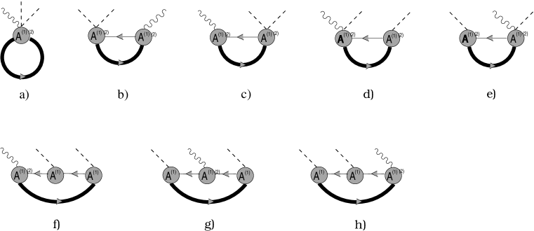
Figure 6: In-medium diagrams with two pions and one photon up to ${\mathcal{O}}(p^{5})$. The analogous diagrams with more than one Fermi-sea insertion are not shown, as they do not contribute here.

$$\langle\pi^{+}\pi^{-}|V^{0}|\Omega\rangle = e\left\{-\frac{\bar{\rho}}{f^{2}}+\frac{g_{A}^{2}{\mathbf{q}}^{2}}{\omega^{2}f^{2}}\bar{\rho}+\omega_{+}({\mathbf{q}})-\omega_{-}({\mathbf{q}})\right\}~{},$$ (5.1)

$$\langle\pi^{+}\pi^{-}|V^{k}|\Omega\rangle = -2e{\mathbf{q}}^{k}\,F_{V}({\mathbf{q}}^{2})\left\{1-\frac{4\hat{\rho}}{f^{2}}c_{2}-\frac{\hat{\rho}+\bar{\rho}}{4m_{N}f^{2}}+\frac{g_{A}^{2}\bar{\rho}}{2m_{N}f^{2}}+\frac{g_{A}^{2}(\hat{\rho}-\bar{\rho})}{4m_{N}f^{2}}\frac{{\mathbf{q}}^{2}}{\omega^{2}}\right\},$$ (5.2)

where $F_{V}({\mathbf{q}}^{2})$ is the vacuum pion vector form factor up to ${\mathcal{O}}(p^{4})$ given in ref. [3]. Note that there is no coupling to a $\pi^{0}\pi^{0}$ state as expected from Bose-Einstein statistics. The term $\omega_{+}({\mathbf{q}})-\omega_{-}({\mathbf{q}})$ in eq. (5.1) arises because of the difference in the energy of the $\pi^{+}$ and $\pi^{-}$ in asymmetric nuclear matter as given by eq. (4.1). Let us stress that the conservation of the electric current, $\partial_{\mu}V^{\mu}=0$, is nontrivial for the in-medium case, as one can find out by studying the origin of the different terms in eq. (5.1). The first one comes from fig. 6a, the second from figs. 6f, g and h while the last two terms originate from from graphs with only two pion lines, without photons, see eqs. (4.1). Despite of that, all of them cancel each other and the temporal derivative is zero as required to guarantee the conservation of the electric current. Indeed if one calculates the matrix element $\langle\pi^{+}\pi^{-}|\partial_{\mu}V^{\mu}|\Omega\rangle$ from eq. (5.1) and (5.2), one obtains:

$$\langle\pi^{+}\pi^{-}|\partial_{\mu}V^{\mu}|\Omega\rangle \propto 2\omega({\mathbf{q}})\left(-\frac{\bar{\rho}}{f^{2}}+\frac{g_{A}^{2}{\mathbf{q}}^{2}}{\omega^{2}f^{2}}\bar{\rho}\right)+\omega_{+}({\mathbf{q}})^{2}-\omega_{-}({\mathbf{q}})^{2}$$ (5.3)

$$= 2\omega({\mathbf{q}})\left(-\frac{\bar{\rho}}{f^{2}}+\frac{g_{A}^{2}{\mathbf{q}}^{2}}{\omega^{2}f^{2}}\bar{\rho}\right)+\left(2\frac{\bar{\rho}}{f^{2}}\omega({\mathbf{q}})-\frac{2g_{A}^{2}\bar{\rho}{\mathbf{q}}^{2}}{f^{2}\omega({\mathbf{q}})}\right)$$

$$= 0~{}.$$

The in-medium contributions to the spatial components of the vector current, eq. (5.2), come from figs. 6a for the first density-dependent term inside the curly brackets, from 6b, c for the second one, and from fig. 6f, g, h for the last two terms. Since it does not involve the non-relativistic suppression factor $1/m_{N}$, the dominant term is the one with the rather large $c_{2}$ counterterm which is also enhanced by a factor of 2 as compared, e.g., to eq. (4.7). The third term in eq. (5.2), figs. 6b and c, involves only the proton density since only protons couple to the photon at this order. The contribution from figs. 6d and e are canceled by those of the wave function renormalization. The last term comes from fig. 6g and this is why it only involves the neutron density. The term before the last one is a combination of figs. 6f and h, with only proton density dependence, and that of fig. 6g.

Figure 7: In-medium pion vector form factor in symmetric nuclear matter as function of the modulus of the pion 3-momentum $q_{\pi\pi}$ (= $|{\bf q}|$). The continuum line is the vacuum ${\mathcal{O}}(p^{4})$ result from ref. [3]. The dashed, dotted and dashed-dotted lines are the in-medium results up to ${\mathcal{O}}(p^{5})$ and correspond to $k_{F}=k_{F}^{0}/2$, $3k_{F}^{0}/4$ and $k_{F}^{0}$, respectively. Note that at $q_{\pi\pi}=0$ the photon virtuality is four times the pion mass squared and that the vacuum form factor is one at virtuality zero.

In fig. 7 we show the in-medium results to the spatial vector coupling in symmetric nuclear matter for three values of $k_{F}$: $k_{F}^{0}/2$, $3k^{0}_{F}/4$ and $k_{F}^{0}$. As stated above, the modifications with density increase rather fast due to the large $c_{2}$ counterterm. Note, however, that the relativistic corrections become more important for higher three-momenta. In fact, the difference between the vacuum ${\mathcal{O}}(p^{4})$ result, solid line, with respect to any of the other lines, gives the in-medium contributions. They rapidly increase as soon as we approach $k_{F}^{0}$ because of the cubic dependence on $k_{F}$ over a quantity of order $k_{F}^{0}$. The lowest order ${\mathcal{O}}(p^{2})$ result is just $1$. Taking the resonance saturation of the $c_{2}$ into account, see ref. [23], one can see that this counterterm just reflects the impact of the $\Delta(1232)$ in low energy $\pi N$ scattering. Thus the term proportional to $c_{2}$ in eq. (5.2), stemming from fig. 6a, establishes a large $\Delta$-hole contribution. Nevertheless, for larger values of the three-momentum $|{\mathbf{q}}|$, the in-medium corrections are relatively less important than the vacuum ones, due to the large $\bar{\ell}_{6}$ CHPT counterterm that signals the well-known and very important $\rho(770)$ contribution to the pion vector form factor in vacuum [3]. Finally note that the form factor in nuclear matter does not go to one at zero virtuality, because this background carries charge.

5.2 Anomalous sector

Since the effective Lagrangian $\widetilde{{\cal L}}_{\pi\pi}$ contains terms with odd number of pions including a $\gamma_{5}$ matrix, one might expect the in-medium appearance of processes violating intrinsic parity, as, e.g., the scattering of three pions or contributions to the $\pi^{0}\rightarrow\gamma\gamma$ decay amplitude. We will show that, up to ${\mathcal{O}}(p^{5})$, there are no in-medium corrections to the $\pi^{0}\rightarrow\gamma\gamma$ amplitude and that the three-pion scattering vanishes in unpolarized nuclear matter at the same order as well.

The set of diagrams to be considered are shown in fig. 8. The figure does not contain any diagram with only one $A$ vertex, as such a contribution is trivially zero. Namely, when $A=A^{(1)}$, it vanishes because then we have one $\gamma_{5}$ matrix together with, at most, two other $\gamma$ matrices, such that the Dirac trace is zero. When $A=A^{(2)}$, the result is zero, simply for the reason that there are no terms in $A^{(2)}$ with two photons and one pion. As indicated in the diagrams of fig. 8, each diagram can contain an $A^{(2)}$ operator attached to a photon line. In fact, one could also have diagrams with just two photon lines stemming from the same $A^{(2)}$ vertex; but they vanish since $[v_{\mu}(x),v_{\nu}(x)]=0$.

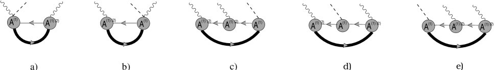
Figure 8: In-medium diagrams with two photon and one pion lines up to ${\mathcal{O}}(p^{5})$. The analogous diagrams with more than one Fermi-sea insertion or with only one $A$ vertex are not shown. Every diagram vanishes independently up to ${\mathcal{O}}(p^{5})$.

Let us show that all the diagrams of fig. 8 vanish. Consider first the diagrams fig. 8a and b with only two leading $A^{(1)}$ operators. It is easy to prove that the flavor trace vanishes for each of them. For this case $\Gamma_{\mu}(x)=-iv_{\mu}(x)$ and $\Delta_{\mu}(x)=-[\phi(x),v_{\mu}(x)]/2$. As a result the flavor traces in figs. 8a,b vanish since:

$$\hat{n}(p)\langle\Gamma_{\mu}(x)\Delta_{\nu}(y)\rangle \rightarrow \langle Q[\phi,Q]\rangle=0~{},$$

$$\bar{n}(p)\langle\tau_{3}\Gamma_{\mu}(x)\Delta_{\nu}(y)\rangle \rightarrow \langle\tau_{3}Q[\phi,Q]\rangle=0~{},$$ (5.4)

where $Q$ is the charge matrix. A change of the order of $\Gamma_{\mu}(x)$ and $\Delta_{\nu}(y)$ in the equations above does not modify the results since $[\tau_{3},Q]=0$. For the same diagrams, but now with one $A^{(2)}$ operator replacing one $A^{(1)}$ operator, there is only a contribution when the other $A^{(1)}=-ig_{A}\gamma^{\mu}\gamma_{5}\Delta_{\mu}$, with $\Delta_{\mu}$ as given above. For the terms in $A^{(2)}$ without gamma matrices the result vanishes, after taking the Dirac trace, because of the $\gamma_{5}$ accompanying $\Delta_{\mu}$ in $A^{(1)}$ and the fact that only three extra gamma matrices are available. The contribution proportional to $c_{4}$ in $A^{(2)}$ vanishes because there are no terms in $u_{\mu}$ involving vector sources without pion fields. Hence two or more pions would arise and this is not allowed. The terms with $c_{6}$ and $c_{7}$ involve the $F^{+}_{\mu\nu}$, which for our present purposes simplifies to $2\partial_{\mu}v_{\nu}-2\partial_{\nu}v_{\mu}$. Thus they only contain the charge matrix $Q$ in flavor space. In summary, when $\Gamma_{\mu}$ is replaced by $F^{+}_{\mu\nu}$, the same reasoning as previously given for the corresponding diagrams with only $A^{(1)}$ operators holds also for this case. The diagrams fig. 8c, d and e deserve special attention, although in the end each of them also vanishes independently at ${\mathcal{O}}(p^{5})$ because of the Dirac trace after symmetrization with respect to the photon lines. Furthermore it is easy to see that the diagrams fig. 8c, d, and e with one $A^{(2)}$ vertex, attached to a $v_{\mu}(x)$ external source, vanish as well. Since these diagrams are at least ${\mathcal{O}}(p^{5})$, one can replace the momentum $p_{j}$ by $p$ inside the expression $\not\mathrel{p}_{j}+m_{N}$, which enters in the numerator of the baryon propagator, because $p_{j}=p+Q_{j}$ and the difference will be ${\mathcal{O}}(p^{6})$. Furthermore, for the same reason, we can set $\not\mathrel{p}$ equal to $\gamma_{0}m_{N}$. Taking also into account that the four-momentum $Q$ of the $\pi^{0}$ is just $(M_{\pi}^{0},\bf{0})$ it is straightforward to see that in all the Dirac traces one has the product $\gamma_{0}(I+\gamma_{0})\gamma_{5}(I+\gamma_{0})=0$ which implies the vanishing of the ${\mathcal{O}}(p^{5})$ contributions from such diagrams.

As a result of this discussion, taking also into account that there are no contributions from diagrams with two or three Fermi-sea insertions because of the reasons discussed in sec. 4.1, the final in-medium $\pi^{0}\rightarrow\gamma\gamma$ decay amplitude $\widetilde{T}(\pi^{0}\rightarrow\gamma\gamma)$, up to ${\mathcal{O}}(p^{5})$, just corresponds to the pure vacuum one given by the Wess-Zumino-Witten term in the effective chiral action [52], counted as ${\mathcal{O}}(p^{4})$ in CHPT. Note also that the corrections to the vacuum phase space induced by the change of the $\pi^{0}$ mass in the medium are at least ${\cal O}(p^{9})$, of the same order as the neglected contributions to the decay resulting from ${\mathcal{O}}(p^{6})$ contributions to $\widetilde{T}(\pi^{0}\rightarrow\gamma\gamma$). Thus up the accuracy we are considering in this paper, there is no modification of the $\pi^{0}\rightarrow\gamma\gamma$ width due to the nuclear medium.

Finally, let us consider the 3$\pi$ scattering, which is not allowed in vacuum, since the anomalous WZW terms only give rise to processes with five or more Goldstone bosons. It turns out that the $3\pi$ scattering does not occur in nuclear matter, at ${\mathcal{O}}(p^{5})$, either.

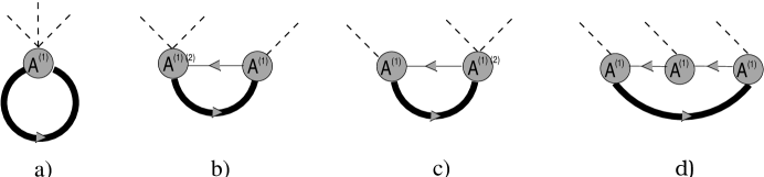
Figure 9: In-medium diagrams with $3\pi$ lines up to ${\mathcal{O}}(p^{5})$. Each of them vanishes independently in asymmetric nuclear matter. The analogous diagrams with more than one Fermi-sea insertion are not shown.

The set of diagrams to be evaluated is depicted in fig. 9. The diagram of fig. 9a vanishes trivially because of the Dirac trace since we have one $\gamma_{5}$ and at most two gamma matrices while at least four gamma matrices are necessary. The latter structure is possible for diagrams fig. 9b,c,d; but in this case one is left with the totally antisymmetric tensor in four dimensions, $\epsilon^{\mu\nu\rho\sigma}$, which requires four independent momenta. However, we have only three of them in any diagram: one is the in-medium running on-shell four-momentum $p$ together with two four-momenta from the pions (the third one is given by energy-momentum conservation). Thus these contributions vanish. Note that only diagrams with just one Fermi-sea insertion are shown in fig. 9, since the proof that each diagram vanishes independently is only based on the Dirac structure of the diagram which is the same independently of whether a free baryon propagator is replaced by a Fermi-sea insertion or not.

6 Four-point Green functions: Pion scattering

The in-medium $4\pi$ scattering contributions begin to appear at ${\mathcal{O}}(p^{3})$ because an in-going pion four-momenta can be combined with an out-going one, such that $Q_{j}^{0}\approx 0$ for one of the propagators. The corresponding diagrams are shown in fig. 10. One can see the ${\mathcal{O}}(p^{3})$ behavior just by applying eq. (2.9), case b). If all the four external pion legs had $Q^{0}\sim k_{F}^{2}/2m_{N}$, then the chiral power counting would start at $\nu=1$ with $V_{\rho}=1$. However, since the pion legs are of course on-shell with $Q^{0}\geq M_{\pi}$, fig. 10a starts at ${\mathcal{O}}(p^{3})$. Indeed, the analysis of all the possible diagrams according to eq. (2.9)-b) up to ${\mathcal{O}}(p^{3})$ shows that the leading contribution corresponding to the diagrams shown in fig. 10 appears at $\nu=3$.

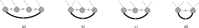
Figure 10: In-medium diagrams contributing to $4\pi$ scattering at ${\mathcal{O}}(p^{3})$. All the vertices are $A^{(1)}$ operators.

Only one Fermi-sea insertion has to be considered in fig. 10. There is no way to include three or four of them, because there is always one four-momentum $Q^{0}\sim M_{\pi}$ running along one insertion that makes it impossible to satisfy $p_{j}^{2}=m_{N}^{2}$ for this thick line, as discussed in sec. 4.1. However, it is in principle possible to have two Fermi-sea insertions. Nevertheless, as shown in sec. 4.1, in this case there is a cancellation, below the Fermi-momentum, between the diagrams with two Fermi-sea insertions and the imaginary parts of those with only one Fermi-sea insertion. It is easy to see that for $Q^{0}=0$ both contributions cancel each other: setting $p_{j}=p+Q$ and then imposing $p_{j}^{2}=m_{N}^{2}$, one can easily see that:

$${\mathbf{Q}}^{2}+2{\mathbf{p}}{\mathbf{Q}}=0~{},$$ (6.1)

since $Q^{0}=0$ and $p^{2}=m_{N}^{2}$. On the other hand, because of the previous cancellations, $|{\mathbf{p}}+{\mathbf{Q}}|>k_{F}$. By squaring this condition and imposing eq. (6.1), one concludes ${\mathbf{p}}^{2}>k_{F}^{2}$ that is not allowed.

In fig. 11 we show some ${\mathcal{O}}(p^{4})$ diagrams that are two connected $3\pi$ scattering processes, which vanish, as already discussed in the previous section, because of the appearance of the totally antisymmetric tensor $\epsilon^{\mu\nu\sigma\rho}$. Nevertheless the vanishing of the diagrams in fig. 11 is due to the pseudoscalar character of the exchanged pion. If instead there were short range NN forces, these diagrams would not only have survived, but would be enhanced by the appearance of nucleon mass factors from each bubble, as discussed in sec. 4.3.

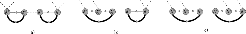
Figure 11: In medium-pion diagrams contributing at ${\mathcal{O}}(p^{4})$. Each of them vanishes independently. More details are given in the text.

In the following we will restrict ourselves to the case of symmetric nuclear matter $\bar{\rho}=0$. The results presented here have been calculated in two ways: using the relativistic formalism from the beginning and performing the chiral expansion up to ${\mathcal{O}}(p^{4})$ afterwards or, from the beginning, making use of those simplifications that are allowed order by order. The results are the same under both ways. Because of the loss of crossing symmetry due to the absence of Lorentz covariance, we consider separately the scattering amplitudes:

$$T_{1}\equiv\pi^{0}\,(q_{1})\pi^{0}\,(q_{2}) \!\!\rightarrow\!\! \pi^{0}\,(q_{3})\pi^{0}\,(q_{4})~{},$$

$$T_{2}\equiv\pi^{+}(q_{1})\pi^{+}(q_{2}) \!\!\rightarrow\!\! \pi^{+}(q_{3})\pi^{+}(q_{4})~{},$$

$$T_{3}\equiv\pi^{+}(q_{1})\pi^{-}(q_{2}) \!\!\rightarrow\!\! \pi^{+}(q_{3})\pi^{-}(q_{4})~{},$$ (6.2)

where $q_{i}$ is the four-momentum of each pion with ${\mathbf{q}}_{1}+{\mathbf{q}}_{2}={\mathbf{q}}_{3}+{\mathbf{q}}_{4}=0$. We further define the three-momenta ${\mathbf{Q}}={\mathbf{q}}_{1}-{\mathbf{q}}_{3}$ and ${\mathbf{R}}={\mathbf{q}}_{1}+{\mathbf{q}}_{3}$ together with the usual Mandelstam variables $s=(q_{1}+q_{2})^{2}=(q_{3}+q_{4})^{2}$, $t=(q_{1}-q_{3})^{2}=(q_{2}-q_{4})^{2}=-{\mathbf{Q}}^{2}$ and $u=(q_{1}-q_{4})^{2}=(q_{2}-q_{3})^{2}=-{\mathbf{R}}^{2}$. It is worthwhile to mention that the ${\mathcal{O}}(p^{4})$ corrections to the leading ${\mathcal{O}}(p^{3})$ diagrams in fig. 10 vanish. Note as well that the in-medium corrections to the pion mass in the symmetric nuclear matter, eq. (4.4), as well as the wave function renormalization, eq. (D.14), appear first at ${\mathcal{O}}(p^{5})$. Then up to ${\mathcal{O}}(p^{3})$ and in the $\rho-$isospin limit $\bar{m}=\bar{\rho}=0$, one has the final expressions:

$$T_{1}(\pi^{0}\,\,\pi^{0}\rightarrow\pi^{0}\,\,\pi^{0}) = \frac{M_{\pi}^{2}}{f_{\pi}^{2}}+\frac{g_{A}^{4}m_{N}tu}{f^{4}\omega^{2}}\left[{\cal I}(0,{\mathbf{Q}})+{\cal I}(0,{\mathbf{R}})\right]~{},$$

$$T_{2}(\pi^{+}\pi^{+}\rightarrow\pi^{+}\pi^{+}) = \frac{2M_{\pi}^{2}-s}{f_{\pi}^{2}}-\frac{4\omega^{2}m_{N}}{f^{4}}\left[{\cal I}(0,{\mathbf{Q}})+{\cal I}(0,{\mathbf{R}})\right]+\frac{4g_{A}^{2}m_{N}}{f^{4}}\Big{\{}\left(t+2\omega^{2}-2M_{\pi}^{2}\right){\cal I}(0,{\mathbf{Q}})$$

$$+ \left(u+2\omega^{2}-2M_{\pi}^{2}\right){\cal I}(0,{\mathbf{R}})\Big{\}}+\frac{2g_{A}^{4}m_{N}}{f^{4}\omega^{2}}\left\{tu-2(\omega^{2}-M_{\pi}^{2})^{2}\right\}\left[{\cal I}(0,{\mathbf{Q}})+{\cal I}(0,{\mathbf{R}})\right]~{},$$

$$T_{3}(\pi^{+}\pi^{-}\rightarrow\pi^{+}\pi^{-}) = \frac{2M_{\pi}^{2}-u}{f_{\pi}^{2}}+\frac{4\omega^{2}m_{N}}{f^{4}}{\cal I}(0,{\mathbf{Q}})-\frac{4g_{A}^{2}m_{N}}{f^{4}}\left\{t+2\omega^{2}-2M_{\pi}^{2}\right\}{\cal I}(0,{\mathbf{Q}})$$ (6.3)

$$+ \frac{4g_{A}^{4}m_{N}}{f^{4}\omega^{2}}(\omega^{2}-M_{\pi}^{2})^{2}{\cal I}(0,{\mathbf{Q}})~{},$$

with $\omega$ the energy of any of the pions and the function ${\cal I}(Q^{0},{\mathbf{Q}})$ as defined in eq. (C). Notice the presence of the $2m_{N}$ factor accompanying the ${\cal I}(0,{\mathbf{Q}})$ and ${\cal I}(0,{\mathbf{R}})$ functions that, as discussed in sec. 4.3, implies a dramatic reduction of the chiral scale $\Lambda$ to about 170 MeV. Nevertheless, one should keep in mind that this scale only refers to the Fermi-momentum $k_{F}$ and the three-momenta $\bf{Q}$ and $\bf{R}$, but not to the energy $\omega$ of the pions which is bounded from below by twice the pion mass. The contributions in eqs. (6) proportional to $g_{A}^{4}$ and $g_{A}^{2}$ come from fig. 10a and fig. 10b,c, respectively. Those stemming from fig. 10d originate from the Weinberg-Tomozawa term and do not contain any $g_{A}$ factor.

Figure 12: From top to bottom: S-wave I=0, P-wave I=1 and S-wave I=2 $\pi\pi$ partial wave amplitudes. The thick full lines are the leading ${\mathcal{O}}(p^{2})$ $\pi\pi$ scattering amplitudes while the thin solid ones are the pure vacuum ${\mathcal{O}}(p^{4})$ results from ref. [3]. The dashed, dotted and dashed-dotted lines are the ${\mathcal{O}}(p^{3})$ in-medium partial wave amplitudes for $k_{F}=100$, 200 and 300 MeV, respectively.

From the previous expressions one can easily work out the in-medium amplitudes with well defined isospin (I) and angular momentum. These are shown in figs. 12 where, from top to bottom, the first panel corresponds to the S-wave I=0 amplitude, the second one to the P-wave I=1 partial wave and the third panel to the S-wave I=2 amplitude, for three values of the Fermi-momentum $k_{F}$ as indicated in the figure. The thick solid curves correspond to the lowest order $\pi\pi$ CHPT partial waves while the thin solid ones to the pure vacuum ${\mathcal{O}}(p^{4})$ $\pi\pi$ amplitudes, ref. [3]. One can see strong in-medium corrections close to threshold for the I=0 and 2 S-waves induced by the diagram of fig. 10d. This diagram only contains the Weinberg-Tomozawa term proportional to $\Gamma_{\mu}$, eq. (B.5), which does not involve a pion three-momenta as is the case for the term proportional to $g_{A}$ in eq. (B.5). This diagram has so far not been considered in the works (see [53, 54, 55]) that are involved in the physics of in-medium pion scattering, triggered by the experimental data of the CHAOS Collaboration [56]. The latter reported originally a dramatic enhancement of the $(\pi^{+},\pi^{+}\pi^{-})$ reaction close to the $2\pi$ threshold, although opposite conclusions have recently been obtained by the Crystal Ball Collaboration [57] from the study of the reaction $(\pi^{-},\pi^{0}\pi^{0})$. It is nowadays believed that when one properly accounts for the limited acceptance of the CHAOS detector, these results are mutually consistent . As one can see, the diagram fig. 10d is indeed dominant for small pion three-momenta, as far as this perturbative analysis holds, since it is not kinematically suppressed as the other contributions with $g_{A}$ dependence because of the P-wave coupling of the pions to the nucleons. At this point it is also worthwhile to note that we have shown explicitly, eq. (6), that the in-medium contribution in symmetric nuclear matter to $\pi\pi$ scattering from the leading pion-nucleon Lagrangian, ${\cal L}^{(1)}_{\pi N}$, does not vanish as stated in ref. [55]. On the other hand, our results for the S-waves, valid for nuclear matter, cannot be taken literally for finite nuclei when $Q^{0}=0$, ${\bf Q}=0$ since the ${\cal I}(Q^{0},{\bf Q})$ function should then vanish due to the finite excitation energy of a few MeV of the nuclear energy levels. This effect is pointed out in ref. [59]. This would imply that in finite nuclei the S-wave I=0 and I=2 amplitudes at threshold do not obtain any contribution from fig. 10d, although, as soon as the pion three-momentum is different from zero, these large corrections rapidly build up. However, as energy increases, the diagrams of fig. 10b and c, which were as well not considered in ref. [53, 54, 55], become more relevant, dominating the in-medium corrections to the P-wave I=1 scattering amplitude. On the other hand, their influence is rather small for the S-waves. The term proportional to $g_{A}^{4}$, fig. 10a, absent as well in refs. [53, 54, 55], is very relevant for the S-waves when the pion three-momentum is higher than 100 MeV, although its influence is much smaller for the P-wave. It is remarkable to point out that for the I=0 and I=1 cases the amplitudes change dramatically with density, while for the I=2 case the S-wave scattering amplitude receives in-medium corrections smaller than those from vacuum ${\mathcal{O}}(p^{4})$ CHPT when $|{\mathbf{q}}|>200$ MeV. Moreover, the I=0 partial waves changes even sign, becoming repulsive, while in the I=1 case there is a strong enhancement as soon as one moves to higher three-momenta and Fermi-momentum. We remind the reader that in the present situation with $Q^{0}_{j}\sim 0$ the perturbative results are only valid for $k_{F}$ and three-momenta up to around $170$ MeV and that the dotted and dashed-dotted lines in fig. 12 are just shown to point out the huge in-medium corrections as soon as one goes beyond that limit, although in the end the actual size of the in-medium corrections depend on the specific reaction. Indeed, for the physics relevant to the CHAOS experiment the effective average density is around $\rho_{0}/2$ [53] corresponding to a $k_{F}\sim 210$ MeV. Hence, one would expect large in-medium non-perturbative effects to take place. Nevertheless, the different models dealing with this problem should match at low densities and momenta with the ${\mathcal{O}}(p^{3})$ results presented in eq. (6) in order to take care of the requirements of chiral symmetry.

7 Conclusions

In this paper we have tackled the problem of establishing a chiral effective field theory in nuclear matter with explicit pion fields. We have made use of the results of ref. [1] where, by integrating out the baryonic fields in the path integral representation of the generating functional, once the change of ground state from vacuum to nuclear matter is done, the in-medium chiral SU(2)$\times$SU(2) Lagrangian is derived. We have briefly reviewed these results in appendix A as well as the perturbative case presenting the corresponding Feynman rules. After establishing the power counting rules, we have systematically studied several low–energy QCD Green functions up to next-to-leading order, ${\mathcal{O}}(p^{5})$, when the standard counting holds or by working out the leading in-medium contributions in the non-standard case. The novel results obtained here can be summarized as follows:

• In contrast to previous works, which apply the mean-field approach or many–body calculations, the in-medium chiral counting is worked out in sec. 2.1. The counting scheme is dependent on the energy flowing into the nucleon lines. This leads one to consider the standard and the non–standard case, respectively, as summarized in table 2. In the former case, the chiral expansion of pion properties in the medium starts with terms at ${\cal O}(p^{4})$, and the next–to–leading order corrections appear at ${\cal O}(p^{5})$, quite different to the in–vacuum power counting.

  	Standard counting	Non-standard counting
  energy flow	$Q^{0}\sim M_{\pi}\sim{\mathcal{O}}(p)$	$Q^{0}\sim Q^{2}/2m_{N}\sim{\mathcal{O}}(p^{2})$
  nucleon propagator	$D_{0}^{-1}\sim{\cal O}(p^{-1})$	$D_{0}^{-1}\sim{\cal O}(p^{-2})$
  counting index $\nu$	eq. (2.4)	eq. (2.9)
  breakdown scale $\Lambda$	$\sqrt{6}\pi f_{\pi}\simeq 0.7\,$GeV	$6\pi^{2}f_{\pi}^{2}/2m_{N}\simeq 0.27\,$GeV

  Table 2: Chiral counting for in–medium CHPT for the standard and the non–standard case. The pertinent breakdown scales are also given. Here, “energy flow” means the energy flowing into the nucleon lines mediated by pions or external sources (as defined in sec. 2.1).

• We have also established the relevant scales of the problem when restricting ourselves to the ${\cal L}_{\pi\pi}$ and ${\cal L}_{\pi N}$ Lagrangians, see sec. 2 or ref. [1]. In the vacuum, the pertinent scale is $\Lambda_{\chi}\simeq 1$ GeV$\sim 4\pi f_{\pi}$. In the medium, one has two new scales. These are: $\sqrt{6}\pi f_{\pi}\simeq 0.7$ GeV and $6\pi^{2}f_{\pi}^{2}/2m_{N}\simeq 0.27$ GeV, in case that the standard or the non-standard counting rules apply, see also table 2. We point out that in case of P-wave interactions, these scales are reduced by factors $1/g_{A}$ and $1/g_{A}^{2}$, respectively.

• We have studied the quark condensates and re-derived, from the effective field theory point of view, known results in symmetric nuclear matter, and have further extended them to the non-symmetric case.

• We have considered the propagation of pions in the medium obtaining the pion propagator up to ${\mathcal{O}}(p^{5})$. In this way we have established that chiral symmetry can account for the observed shift of the mass of the negative pion in deeply bound pionic states in ²⁰⁷Pb. Our numerical result $\Delta M_{\pi^{-}}=18\pm 5\,$MeV is compatible with the experimental number, $\Delta M_{\pi^{-}}=23-27\,$MeV [6, 7] within errors.

• The wave function renormalization of the pion fields corresponding to the calculated in-medium action $\int dx\widetilde{{\cal L}}$ has been established making use of first principles.

• We have also studied the coupling of pions with axial-vector and pseudoscalar sources. In particular, it is shown that in-medium corrections up to ${\mathcal{O}}(p^{5})$ do not spoil the validity of the Gell-Mann-Oakes-Renner relation. We have also found a decrease with increasing density for both the quark condensates and the temporal component of the pion decay constant $f_{t}$. Both effects seem to indicate a partial chiral symmetry restoration with increasing density. We remark again that a systematic study of the in-medium order parameters still has to be performed. A drastic quenching with density has also been obtained for the spatial component of the pion decay constant $f_{s}$. To ${\mathcal{O}}(p^{5})$ we have checked the QCD Ward identity relating both the temporal and spatial components of the axial-vector currents with the pseudoscalar ones and quark masses.

• A rapid decrease with density of the coupling of a photon to two pions, particularly in the threshold region, has been found. The derived vector current amplitudes coupled to two pions fulfill the requirement of current conservation. Furthermore, we have established the absence of in-medium renormalization up to ${\mathcal{O}}(p^{5})$ of the anomalous $\pi^{0}\rightarrow\gamma\gamma$ decay amplitude.

• Finally, $\pi\pi$ scattering has been studied up to ${\mathcal{O}}(p^{3})$ since in this case the non-standard counting occurs. As explained in secs. 2.1 and 6, this implies that the in-medium corrections start at lower orders than in the standard case, here already at ${\mathcal{O}}(p^{3})$. In addition the scale, below which the perturbative expansion is applicable, decreases. As a result the in-medium corrections increase very rapidly with density and already at $k_{F}\simeq 200$ MeV, or at a density of just $\sim 0.4\rho_{0}$, they are $100\%$ with respect to the lowest order CHPT results. The diagrams presented in figs. 10 are the leading ones in the chiral expansion and have not been considered so far in the literature.

Future challenges are the inclusion of multi-nucleon contact interactions, which are enhanced because of the largeness of the S-wave scattering lengths related to the presence of shallow NN bound states, as well as the simultaneous calculation of pion loops necessary for determination of the full ${\mathcal{O}}(p^{6})$ contributions. Furthermore, the possibility of some non-perturbative scheme that allows for the recovery of the scale $\sqrt{6}\pi f_{\pi}$, even in the case of the non-standard counting or when the multi-nucleon local interactions are included, should be pursued.

Acknowledgments

We would like to thank E. Oset for useful discussions. The work of J.A.O. was supported in part by funds from DGICYT under contract PB96-0753 and from the EU TMR network Eurodaphne, contract no. ERBFMRX-CT98-0169.

Appendix A Generating functional

Our starting point is the generating functional ${\cal Z}(v,a,s,p)$ in the presence of external vector $v$, axial–vector $a$, scalar $s$ and pseudoscalar $p$ sources (included in ${\cal L}_{\pi\pi}$ and ${\cal L}_{\pi N}$) which is obtained after integrating out the baryonic fields, as derived in ref. [1] (for all details on the derivation, we refer to that paper). It is given by

$$e^{i{\cal Z}[v,a,s,p]}\!\!\! = \!\!\!\int\![dU]\exp\Bigg{\{}i\!\int\!dx\,{\cal L}_{\pi\pi}\!$$

$$- i\!\int\!\frac{d{\mathbf{p}}}{(2\pi)^{3}2E(p)}\!\int\!dx\,dy\,e^{ip(x-y)}\,\hbox{Tr}\Bigg{(}A[I_{4}-D_{0}^{-1}A]^{-1}\arrowvert_{(x,y)}(\not\mathrel{p}+m_{N})\,n(p)\Bigg{)}$$

$$+ \frac{1}{2}\!\int\!\!\!\frac{d{\mathbf{p}}}{(2\pi)^{3}2E(p)}\!\int\!\!\!\frac{d{\mathbf{q}}}{(2\pi)^{3}2E(q)}\!\int\!dx\,dx^{\prime}\,dy\,dy^{\prime}\,e^{ip(x-y)}e^{-iq(x^{\prime}-y^{\prime})}\,$$

$$\times \hbox{Tr}\Bigg{(}A[I_{4}-D_{0}^{-1}A]^{-1}\arrowvert_{(x,x^{\prime})}\,(\not\mathrel{q}+m_{N})n(q)A[I_{4}-D_{0}^{-1}A]^{-1}\arrowvert_{(y^{\prime},y)}(\not\mathrel{p}+m_{N})\,n(p)\Bigg{)}+...\Bigg{\}}~{},$$

where the trace, indicated by Tr, is over the spinor and flavor indices. From this result we can readily read off the new effective chiral Lagrangian density $\widetilde{{\cal L}}_{\pi\pi}$ in the presence of nucleonic densities just by equating the expression between curly brackets to $i\int dx\widetilde{{\cal L}}_{\pi\pi}$. Furthermore, the diagonal flavor matrix $n(p)$ in eq. (A) is:

$$n(p) = \left(\begin{array}[]{cc}\theta(k_{F}^{(p)}-|{\mathbf{p}}|)&0\\ 0&\theta(k_{F}^{(n)}-|{\mathbf{p}}|)\end{array}\right)\equiv\left(\begin{array}[]{cc}n(p)_{1}&0\\ 0&n(p)_{2}\end{array}\right)=\hat{n}(p)I_{2}+\bar{n}(p)\tau_{3}~{},$$ (A.6)

with $I_{2}$ the $2\times 2$ unity matrix, $\theta(x)$ the Heaviside step function, $\tau_{3}$ the usual Pauli matrix, $\tau_{3}={\rm diag}(1,-1)$, $\hat{n}(p)=(n(p)_{1}+n(p)_{2})/2$ and $\bar{n}(p)=(n(p)_{1}-n(p)_{2})/2$. We are considering the general case of asymmetric nuclear matter with two Fermi-seas of protons and neutrons with densities $\rho^{p}=(k_{F}^{(p)})^{3}/3\pi^{2}$ and $\rho^{n}=(k_{F}^{(n)})^{3}/3\pi^{2}$, respectively, with $k_{F}^{(p)}$ and $k_{F}^{(n)}$ the corresponding Fermi momenta. In eq. (A) the nucleon energy is given by $E(p)=\sqrt{{\mathbf{p}}^{2}+m_{N}^{2}}$, where $m_{N}=(m_{n}+m_{p})/2\simeq 939$ MeV, since the difference between the proton and neutron masses is ${\mathcal{O}}(p^{2})$ giving rise to in-medium contributions of higher order than the next-to-leading order ones, see section 2.1. For the same reason, we will also use the average nucleon mass, $m_{N}$, in the baryon propagators.

The ellipses in eq. (A) indicate terms with a higher number of three-momentum integrals over the Fermi-seas coming from a logarithmic expansion of the vacuum interaction operator $\Gamma=-iA[I_{4}-D_{0}^{-1}]^{-1}$[1]. Notice that the Fermi-sea states are on-shell, $p^{0}=E(p)$. Indeed, for $n\geq 1$ Fermi-sea insertions one picks up a factor $(-1)^{n+1}/n$, while every operator $\Gamma=-iA[I_{4}-D_{0}^{-1}]^{-1}$, containing both pion legs and external sources, implies a phase of $-i$ . The operator $A$ is defined as follows:

$$\int dx\,{\cal L}_{\pi N}=\int dx\,\bar{\psi}(x)D(x)\psi(x)=\int dx\,\bar{\psi}(x)D_{0}(x)\psi(x)-\int dx\,dy\,\bar{\psi}(x)A(x,y)\psi(y)~{},$$ (A.7)

where $D_{0}(x)=i\gamma^{\mu}\partial_{\mu}-M_{N}$ is the free Dirac operator and the symbol $M_{N}$ refers to the diagonal matrix $M_{N}={\rm diag}(m_{p},m_{n})$ of physical proton and neutron masses, respectively. Hence, standard in-medium generalized vertices from eq. (A) can be represented as in fig. 1 where each connected diagram represents one of such vertices and the vacuum non-local vertices $\Gamma$ are connected through the exchange of on-shell Fermi-sea states. The latter are represented by the thick solid lines in that and all following diagrammatic figures. Furthermore, $\Gamma$ results from the iteration of the $-iA$ operator with intermediate free baryon propagators $iD_{0}^{-1}$ as shown in fig. 2. Consequently, any diagram with medium contributions will be a set of $V_{\rho}\geq 1$ generalized in-medium vertices. For each of them one has $n_{j}\geq 1$ Fermi-sea insertions, $1\leq j\leq V_{\rho}$, $m_{j}\geq 0$ free baryon-propagators and of $m_{j}+n_{j}$ vertices $-iA$. The resulting Feynman rules (as derived in [1]) read:

• First include the global sign $(-1)^{V_{\rho}}$ because of the fermionic closed loop attached to each generalized vertex, and the combinatoric sign factor

  $$\prod_{j=1}^{V_{\rho}}\frac{(-1)^{n_{j}}}{n_{j}}$$ (A.8)

  from the logarithmic expansion giving rise to the different in-medium vertices.

• Then, following the vertex in the opposite sense to that of the fermionic arrows, write for each Fermi-sea insertion an integral

  $$\int\!\!\frac{d{\mathbf{p}}\,(\not\mathrel{p}+m_{N})}{(2\pi)^{3}2E(p)}n(p)$$ (A.9)

  with $p^{0}=E(\mathbf{p})$ and for every vacuum baryon propagator with free momentum $p$ write

  $$i\int\!\!\frac{dp}{(2\pi)^{4}}\frac{\not\mathrel{p}+m_{N}}{p^{2}-m_{N}^{2}+i\epsilon}~{}.$$ (A.10)

• For a vertex in momentum space write a term

  $$-iA\,(2\pi)^{4}~{},$$ (A.11)

  keeping in mind the energy-momentum conservation at each vertex.

• Then for each pion internal line write the pion vacuum propagator

  $$i\int\frac{dq}{(2\pi)^{4}}\frac{1}{q^{2}-M_{\pi}^{2}+i\epsilon}~{}.$$ (A.12)

• Finally, sum over the Dirac and spin indices of the fermions.

This defines explicitly the Feynman rules in momentum space in order to obtain $i(2\pi)^{4}$ times the desired connected graph accompanied by the global delta function of energy-momentum conservation. It is important to keep in mind that a generalized vertex behaves as a standard local one of quantum field theory with respect to the determination of the numerical factors accompanying a given diagram under the exchange of pions. This can be seen by simply applying standard perturbative techniques in path integrals to the action given between brackets in eq. (A). It is also worthwhile to note that one can take eq. (A) directly in configuration space, see sections 3 and 4.1 and the appendix D.

Appendix B Chiral Lagrangians and the interaction operators $A^{(1)}$ and $A^{(2)}$

To evaluate the next-to-leading order medium corrections to the Green functions from the $\pi N$ Lagrangian ${\cal L}_{\pi N}=\bar{\psi}D(x)\psi$, as discussed in detail in sec. 2.1, one has to consider the ${\mathcal{O}}(p)$ ${\cal L}^{(1)}_{\pi N}$ and ${\mathcal{O}}(p^{2})$ ${\cal L}^{(2)}_{\pi N}$ Lagrangians. For relativistic spin-1/2 fields chirally coupled to pions and external sources, the lowest order effective Lagrangian reads [22]

$${\cal L}_{\pi N}^{(1)}=\bar{\psi}\left(i\gamma^{\mu}\partial_{\mu}-\stackrel{{\scriptstyle\circ}}{{m}}_{N}\!I_{2}+i\gamma^{\mu}\Gamma_{\mu}+i\stackrel{{\scriptstyle\circ}}{{g}}_{A}\gamma^{\mu}\gamma_{5}\Delta_{\mu}\right)\psi~{},$$ (B.1)

with $\Delta_{\mu}=\frac{1}{2}u^{\dagger}\nabla_{\mu}\!U\,u^{\dagger}$ in terms of the covariant derivative $\nabla_{\mu}U(x)=\partial_{\mu}U(x)-i(v_{\mu}(x)+a_{\mu}(x))U(x)+iU(x)(v_{\mu}(x)-a_{\mu}(x))$. $\Gamma_{\mu}$ is the chiral connection, $\Gamma_{\mu}=\frac{1}{2}\left[u^{\dagger},\partial_{\mu}u\right]-\frac{i}{2}u^{\dagger}(v_{\mu}+a_{\mu})u-\frac{i}{2}u(v_{\mu}-a_{\mu})u^{\dagger}$. The Goldstone bosons (the pions) are collected in the $2\times 2$ unitary matrix $u=\exp(i\phi/2f)$, $U=u^{2}$ and $\phi$ is given by:

$$\phi=\left(\begin{array}[]{cc}\pi^{0}&\sqrt{2}\pi^{+}\\ \sqrt{2}\pi^{-}&-\pi^{0}\end{array}\right).$$ (B.4)

On the other hand, the constants $\stackrel{{\scriptstyle\circ}}{{m}}_{N}$, $\stackrel{{\scriptstyle\circ}}{{g}}_{A}$ and $f$ refer to the mass, axial coupling of the nucleon and weak pion decay constant in the SU(2) chiral limit. Taking into account the definition of the $A$ operator, $A(x)\equiv D_{0}(x)-D(x)$, with $D_{0}(x)=i\gamma^{\mu}\partial_{\mu}-M_{N}$, we obtain from eq. (B.1) for the first term in the chiral expansion of the operator $A$,

$$A^{(1)}=-i\gamma^{\mu}\Gamma_{\mu}-i\stackrel{{\scriptstyle\circ}}{{g}}_{A}\gamma^{\mu}\gamma_{5}\Delta_{\mu}~{}.$$ (B.5)

The difference $\stackrel{{\scriptstyle\circ}}{{m}}_{N}\!I_{2}-M_{N}$ is ${\mathcal{O}}(p^{2})$ [22] and will be included in $A^{(2)}$. Although strictly speaking there is no explicit symmetry breaking at leading order in the effective pion–nucleon Lagrangian, this identification will turn out to be convenient at later stages.

To obtain the complete expression of the (second order) $A^{(2)}$ operator, we have to take into account the Lagrangian ${\cal L}^{(2)}_{\pi N}$ (we use here the notation of ref. [34]). The operator $A^{(2)}$ can be obtained by just removing the $\psi$ and $\bar{\psi}$ fields from the Lagrangian and by changing the overall sign,

$$A^{(2)} = \stackrel{{\scriptstyle\circ}}{{m}}_{N}\!I_{2}-M_{N}-c_{1}\langle\chi_{+}\rangle+\frac{c_{2}}{2\stackrel{{\scriptstyle\circ}}{{m}}_{N}^{2}}\langle u_{\mu}u_{\nu}\rangle D^{\mu}D^{\nu}-\frac{c_{3}}{2}\langle u_{\mu}u^{\mu}\rangle+\frac{c_{4}}{4}\gamma^{\mu}\gamma^{\nu}[u_{\mu},u_{\nu}]-c_{5}\,\hat{\chi}_{+}$$ (B.6)

$$- \frac{ic_{6}}{8\stackrel{{\scriptstyle\circ}}{{m}}_{N}}\gamma^{\mu}\gamma^{\nu}F_{\mu\nu}^{+}-\frac{ic_{7}}{8\stackrel{{\scriptstyle\circ}}{{m}}}\gamma^{\mu}\gamma^{\nu}\langle F_{\mu\nu}^{+}\rangle~{},$$

where the ${\mathcal{O}}(p^{2})$ low-energy constants $c_{i}$ are finite and where we have also added the term $\stackrel{{\scriptstyle\circ}}{{m}}_{N}\!I_{2}-M_{N}$ as discussed above. Furthermore, we have $D_{\mu}=\partial_{\mu}+\Gamma_{\mu}$, $u_{\mu}=2i\Delta_{\mu}$, $\chi_{+}=u^{\dagger}\chi u^{\dagger}+u\chi^{\dagger}u$ with $\chi(x)=2B_{0}(s(x)+ip(x))$. Here, $B_{0}\,\delta^{ij}=-\langle 0|\bar{q}^{i}q^{j}|0\rangle/f^{2}$ measures the strength of the symmetry breaking in the chiral limit. The quark mass matrix ${\cal M}={\rm diag}(m_{u},m_{d})$ is included in the scalar source $s(x)={\cal M}+\cdot\cdot\cdot$. The trace in flavor space of an arbitrary matrix ${\cal O}$ is denoted by $\langle{\cal O}\rangle$. In this way, the traceless matrix $\hat{\chi}_{+}$ is defined as $\hat{\chi}_{+}=\chi_{+}-\frac{1}{2}\langle\chi_{+}\rangle$. Finally, $F_{\mu\nu}^{+}=u^{\dagger}F_{\mu\nu}^{R}u+uF_{\mu\nu}^{L}u^{\dagger}$ where $F_{\mu\nu}^{L}=\partial_{\mu}\ell_{\nu}-\partial_{\nu}\ell_{\mu}-i[\ell_{\mu},\ell_{\nu}]$, $F_{\mu\nu}^{R}=\partial_{\mu}r_{\nu}-\partial_{\nu}r_{\mu}-i[r_{\mu},r_{\nu}]$ with $\ell_{\mu}=v_{\mu}-a_{\mu}$ and $r_{\mu}=v_{\mu}+a_{\mu}$. For more details see e.g. ref. [34]. We briefly collect the chiral power (or chiral dimension) of the basic ingredients that appear repeatedly in the chiral expansion of the operator $A$. Namely, $\partial_{\mu}u$, $v_{\mu}$ and $a_{\mu}$ are $\sim{\mathcal{O}}(p)$ while $s$, $p$, $\chi$ and $F_{\mu\nu}^{L,R}$ are $\sim{\mathcal{O}}(p^{2})$. On the other hand, $u$ and $\partial_{\mu}\psi$ $\sim{\cal O}(1)$ (although $\partial_{i}\psi$ $\sim{\mathcal{O}}(p)$ for the spatial components $i$). We point out that the first two terms in eq. (B.6) appear because the free Dirac operator $D_{0}$ is defined in terms of the physical nucleon masses (and not the mass in the chiral limit). It is straightforward to show that up to ${\mathcal{O}}(p^{2})$ in $A^{(2)}$, the difference $\stackrel{{\scriptstyle\circ}}{{m}}_{N}\!I_{2}-M_{N}$ is canceled by the constant contributions coming from the terms proportional to $c_{1}$ and $c_{5}$. Up to ${\mathcal{O}}(p^{2})$, it is easy to work out from the Lagrangians ${\cal L}_{\pi N}^{(1)}$ and ${\cal L}_{\pi N}^{(2)}$ the following expressions for the masses of protons, $m_{p}$, and neutrons, $m_{n}$:

$$m_{p} = \stackrel{{\scriptstyle\circ}}{{m}}_{N}-8B_{0}c_{1}\hat{m}-4B_{0}c_{5}\bar{m}~{},$$

$$m_{n} = \stackrel{{\scriptstyle\circ}}{{m}}_{N}-8B_{0}c_{1}\hat{m}+4B_{0}c_{5}\bar{m}~{},$$ (B.7)

where $\hat{m}=(m_{u}+m_{d})/2$ is the average light quark mass and $\bar{m}=(m_{u}-m_{d})/2$ measures the strength of strong isospin breaking. When inserting the previous expressions in eq. (B.6) the difference $\stackrel{{\scriptstyle\circ}}{{m}}_{N}\!I_{2}-M_{N}$ will cancel those terms from $c_{1}$ and $c_{5}$ that are independent of the quantum pion fields or the external sources $v$, $a$, $s$ and $p$. Indeed one can generalize this result for any $A^{(n)}$ operator, with $n\geq 2$, following similar arguments to the ones given in ref. [34]. Among the building blocks for the construction of a chiral ${\cal L}_{\bar{\psi}\psi}$ Lagrangian, only the scalar operator $\chi_{+}$ gives rise to terms without pion or external source legs, leading to a constant matrix. Given $\chi_{+}$, one can then build up operators ${\cal O}$ to be sandwiched between the $\bar{\psi}$ and $\psi$ fields which give rise to constant matrices without any field. In addition, one can include any number of covariant derivatives $D_{\mu}$, since they count as ${\cal O}(1)$ and the partial derivative $\partial_{\mu}$, contained in $D_{\mu}$, does not include any pion or external source in contrast to $\Gamma_{\mu}$. However, we can integrate by parts in such a way, that all the $\partial_{\mu}$ act either to the left or to the right of the $\chi_{+}$, as otherwise they will give rise to vertices with at least one pion or external leg. When all the Lorentz indices of these operators are contracted with the $\gamma-$matrices, the metric tensor and the totally antisymmetric tensor in $d=4$ dimensions [34], it follows from the application of the equations of motions and from the trivial result $\left[\partial_{\mu},\partial_{\nu}\right]=0$ that the $\partial_{\mu}$ operators in the covariant derivatives just give rise to factors of $\stackrel{{\scriptstyle\circ}}{{m}}$. These factors can be reabsorbed in the couplings of those operators that are only constructed from $\chi_{+}$ or in the vertices with one or more legs. As a result all the vertices without any legs are just constant and their finite parts are reabsorbed in the definition of the physical nucleon mass matrix $M_{N}$. The infinite parts that could arise because of possible scale dependent counterterms in front of such terms, needed for the renormalization, have to be considered jointly with pions loops, which obviously involve pion legs.

Appendix C Application of the non-standard counting rules to in-medium pion propagation

As an illustration we will discuss the application of the non–standard power counting in detail, as it appears for the in-medium pion-propagation. The leading contribution is ${\mathcal{O}}(p^{3})$ and contains one generalized vertex, $V_{\rho}=1$ at lowest order, $\delta_{1}=4$, while $V_{\pi}=0$, $n_{m}=0$ for $m\geq 2$ and $I_{B}=I_{B}^{\star}$. Obviously $p_{m}=0$ for all $m$ since $V_{\pi}=0$. This case corresponds to figs. 5a, where only one Fermi-sea line has been shown although it should be clear that one can substitute any thin line by a thick one including the appropriate factors as discussed in detail in appendix A, in sec. 4.1 and in ref. [1]. The next-to-leading order is then ${\mathcal{O}}(p^{4})$ and there are various contributions:

1. The same as before but with $\Delta I_{B}\equiv I_{B}-I_{B}^{\star}=1$. This corresponds to fig. 5.b. Other diagrams similar to this one obtained just by exchanging the positions of the lines and the loop are not shown. Instead of a loop one can also have an ${\mathcal{O}}(p^{3})$ $\pi N$ counterterm without pion lines just for renormalization, as discussed at the end of sec. B.

2. $V_{\rho}=1$, $\delta_{1}=4$, $V_{\pi}=0$, $n_{2}=1$ and $\Delta I_{B}=0$. This gives rise to the diagrams in fig. 5c,d, where, as before, diagrams obtained under the exchange of the positions of lines and the loop or by the inclusion of any extra Fermi-sea insertion are not explicitly shown. The diagram of fig. 5d is zero because the Weinberg term with two pions involves the vertex $\left[\phi,\partial_{\mu}\phi\right]=2i\epsilon_{ijk}\phi_{i}\partial_{\mu}\phi_{j}$, and hence one cannot have the same two flavors in one vertex.

3. $V_{\rho}=2$, $\delta_{1,2}=4$, $V_{\pi}=0$, $n_{m}=0$ $m\geq 2$ and $\Delta I_{B}=0$. The diagrams are shown in figs. 5e,f. As before diagrams obtained by exchanging lines and adding more Fermi-sea insertions are not shown. The diagram in fig. 5f vanishes because the new generalized vertex with only one pion is zero since there is a $\gamma_{5}$ matrix from the pion vertex and at most two additional gamma matrices.

It is worthwhile to mention that in this example there is no contribution at next-to-leading order from the insertion of one $A^{(2)}$ operator in a generalized in-medium vertex, because then there are at least two pion lines involved, so that $\delta_{1}=5$ and $n_{2}=1$. As a result such contributions only start at ${\mathcal{O}}(p^{5})$.

In order to calculate the diagram in fig. 5a one has to make use of the full baryon propagator and not the heavy baryon (HB) expansion in eq. (2.1). We have calculated this diagram for the case of symmetric nuclear matter, where, as discussed above, the diagram fig. 5c vanishes as well. Then, up to ${\mathcal{O}}(p^{3})$ and for $\bar{\rho}=0$, we have instead of eqs. (4.1):

$$\omega^{2}-{\mathbf{Q}}^{2}-M_{\pi}^{2}+\frac{2m_{N}g_{A}^{2}Q^{2}}{f^{2}}\left({\cal I}(\omega,{\mathbf{Q}})+{\cal I}(-\omega,{\mathbf{Q}})\right)$$

$$-i\frac{g_{A}^{2}Q^{2}m_{N}}{2\pi f^{2}}\left(\theta(\omega)\theta(k_{F}^{2}-2m_{N}\omega)\theta(k_{F}-k_{M}(\omega))\frac{k_{F}^{2}-k^{2}_{M}(\omega)}{4|{\mathbf{Q}}|}+\omega\rightarrow-\omega\right)=0~{},$$ (C.1)

where $k^{2}_{M}(\omega)$ is the maximum of $k_{F}^{2}-2m_{N}\omega$ and $(Q^{2}+2m_{N}\omega)^{2}/4{\mathbf{Q}}^{2}$. The function ${\cal I}(Q^{0},{\mathbf{Q}})$ is given by:

$${\cal I}(Q^{0},{\mathbf{Q}}) = {\cal P}\int^{k_{F}}\!\!\!\!\frac{d\mathbf{p}}{(2\pi)^{3}}\frac{1}{Q^{2}+2m_{N}Q^{0}-2{\mathbf{p}}{\mathbf{Q}}}$$

$$= \frac{k_{F}(Q^{2}+2m_{N}Q^{0})}{16\pi^{2}{\mathbf{Q}}^{2}}+\frac{(Q^{2}+2m_{N}Q^{0})^{2}-4k_{F}^{2}{\mathbf{Q}}^{2}}{128\pi^{2}|{\mathbf{Q}}|^{3}}\log\frac{(Q^{2}+2m_{N}Q^{0}-2k_{F}|{\mathbf{Q}}|)^{2}}{(Q^{2}+2m_{N}Q^{0}+2k_{F}|{\mathbf{Q}}|)^{2}}~{},$$

where ${\cal P}$ indicates the principal value of the integral. The step functions in eq. (C) stem from the interplay of the second Fermi-sea insertion in fig. 4c with the pole from the free baryon propagator in fig. 4b as discussed in sec. 4.1.

Appendix D Wave function renormalization

The pion fields are naturally normalized by imposing the canonical commutation relations at equal times $x^{0}=y^{0}$:

$$\left[\pi(x)^{\alpha},\widetilde{\Pi}(y)^{\beta}\right]=i\delta({\mathbf{x}}-{\mathbf{y}})\delta^{\alpha\beta}~{},$$

$$\left[\pi(x)^{\alpha},\pi(y)^{\beta}\right]=\left[\widetilde{\Pi}(x)^{\alpha},\widetilde{\Pi}(y)^{\beta}\right]=0~{},$$ (D.1)

where the indices $\alpha$, $\beta$ can refer to any of the $\pi^{0}$, $\pi^{+}$ and $\pi^{-}$ fields and $\widetilde{\Pi}(x)^{\alpha}$ is the conjugate momentum of the field $\pi(x)^{\alpha}$. We now proceed to calculate the in-medium pion field and conjugate momentum from the quadratic term in the pion fields, $\int dx\widetilde{{\cal L}}_{\phi\phi}$, of $\int dx\widetilde{{\cal L}}$.

The in-medium free pion fields are given, at the classical level, by the equations of motion,

$$\delta\int dx\widetilde{{\cal L}}_{\phi\phi}/\delta\phi_{k}(y)=0~{},$$

already discussed in sec. 4.1. These are fulfilled by writing the pion fields as:

$$\pi^{+}(x) = \int\frac{d{\bf Q}}{(2\pi)^{3}}\left[a({\mathbf{Q}})e^{-iQx}+b^{\dagger}({\mathbf{Q}})e^{i{\widetilde{Q}}x}\right]~{},$$

$$\pi^{-}(x) = \int\frac{d{\bf Q}}{(2\pi)^{3}}\left[b({\mathbf{Q}})e^{-i{\widetilde{Q}}x}+a^{\dagger}({\mathbf{Q}})e^{iQx}\right]~{},$$

$$\pi^{0}(x) = \int\frac{d{\bf P}}{(2\pi)^{3}}\left[c({\mathbf{P}})e^{-iPx}+c^{\dagger}({\mathbf{P}})e^{iPx}\right]~{},$$ (D.2)

where $Q^{0}({\mathbf{Q}}^{2})=\omega_{+}({\mathbf{Q}}^{2})$, ${\widetilde{Q}}^{0}({\mathbf{Q}}^{2})=\omega_{-}({\mathbf{Q}}^{2})$ and $P^{0}({\mathbf{P}}^{2})=\omega_{0}({\mathbf{Q}}^{2})$ are positive functions of the square of the three-momentum and correspond, respectively, to the $\pi^{+}$, $\pi^{-}$ and $\pi^{0}$ energies and are given by the corresponding spectral relation between energy and three-momentum, eqs. (4.1). Note that in eqs. (D) we have space-time dependences of the form $e^{-iQx}$ and $e^{iQx}$. When applying eqs. (4.1) to the latter case, we have to substitute $Q^{0}\rightarrow-Q^{0}$ since these formulae were deduced taking a generic form $e^{-iQx}$ and allowing for both positive as well as negative values of $Q^{0}\equiv\omega$. Taking this into account, together with the fact that the terms proportional to $\bar{\rho}$ in eqs. (4.1) are odd in $\omega$, we can then combine the coefficients $a({\mathbf{Q}})$ and $b({\mathbf{Q}})$ and their conjugates in the $\pi^{+}$ and $\pi^{-}$ fields as shown in eqs. (D). On the other hand, the in-medium contribution to the pion conjugate momenta $\widetilde{\Pi}_{i}(x)$ are calculated by differentiating the quadratic piece $\int dx\delta\widetilde{{\cal L}}_{\phi\phi}$ (given up to ${\mathcal{O}}(p^{5})$ and times a factor of $i$ in eq. (4.1)) with respect to $\dot{\phi}(x)_{i}$. In order to deal with the presence of the non-localities induced by the baryon propagator $D_{0}^{-1}(x,y)$, we have worked in momentum space after calculating the functional derivative. Proceeding in this way, one finds for $\widetilde{\Pi}_{i}(x)$:

$$\widetilde{\Pi}(x)_{i} = \dot{\phi}(x)_{i}\left\{1+\frac{4\hat{\rho}}{f^{2}}\left(c_{2}+c_{3}-\frac{g_{A}^{2}}{8m_{N}}\right)\right\}+\sum_{k=1}^{3}\epsilon_{ik3}\frac{\bar{\rho}}{2f^{2}}\phi_{k}(x)$$ (D.3)

$$- i\frac{g_{A}^{2}\hat{\rho}}{2m_{N}f^{2}}\int\frac{d{\mathbf{Q}}}{(2\pi)^{3}}\,\frac{{\mathbf{Q}}^{2}}{2\omega_{{\rm vac}}({\mathbf{Q}}^{2})^{2}}\left[\phi_{i}({\mathbf{Q}})e^{-iQx}\!-\!\phi_{i}({\mathbf{Q}})^{\dagger}e^{iQx}\right]~{},$$

where we have denoted the vacuum energy by $\omega_{{\rm vac}}({\mathbf{Q}}^{2})=\sqrt{M_{\pi}^{2}+{\mathbf{Q}}^{2}}$. One can easily calculate the conjugate momenta of the fields $\pi^{+}(x)$, $\pi^{-}(x)$ and $\pi^{0}(x)$ from eq. (D.3). Taking also into account eqs. (D) one has:

$$\widetilde{\Pi}(x)^{+} \!\!\!=\!\!\! -i\int\frac{d{\mathbf{Q}}}{(2\pi)^{3}}\left[\omega_{-}({\mathbf{Q}}^{2})b({\mathbf{Q}})e^{-i{\widetilde{Q}}x}-\omega_{+}({\mathbf{Q}}^{2})a^{\dagger}({\mathbf{Q}})e^{iQx}\right]\left\{1+\frac{4\hat{\rho}}{f^{2}}\left(c_{2}+c_{3}-\frac{g_{A}^{2}}{8m_{N}}\frac{M_{\pi}^{2}}{\omega_{{\rm vac}}({\mathbf{Q}}^{2})^{2}}\right)\right\}$$

$$- i\frac{\bar{\rho}}{2f^{2}}\pi^{-}(x)~{},$$

$$\widetilde{\Pi}(x)^{-} \!\!\!=\!\!\! -i\int\frac{d{\mathbf{Q}}}{(2\pi)^{3}}\left[\omega_{+}({\mathbf{Q}}^{2})a({\mathbf{Q}})e^{-iQx}-\omega_{-}({\mathbf{Q}}^{2})b^{\dagger}({\mathbf{Q}})e^{i{\widetilde{Q}}x}\right]\left\{1+\frac{4\hat{\rho}}{f^{2}}\left(c_{2}+c_{3}-\frac{g_{A}^{2}}{8m_{N}}\frac{M_{\pi}^{2}}{\omega_{{\rm vac}}({\mathbf{Q}}^{2})^{2}}\right)\right\}$$

$$+ i\frac{\bar{\rho}}{2f^{2}}\pi^{+}(x)~{},$$

$$\widetilde{\Pi}(x)^{0} = -i\int\frac{d{\mathbf{P}}}{(2\pi)^{3}}\omega_{0}({\mathbf{P}}^{2})\left[c({\mathbf{P}})e^{-iPx}-c^{\dagger}({\mathbf{P}})e^{iPx}\right]\left\{1+\frac{4\hat{\rho}}{f^{2}}\left(c_{2}+c_{3}-\frac{g_{A}^{2}}{8m_{N}}\frac{M_{\pi}^{2}}{\omega_{{\rm vac}}({\mathbf{P}}^{2})^{2}}\right)\right\}~{}.$$

We now proceed to the quantization of the pion fields eqs. (D) by imposing the canonical commutation relations given in eqs. (D) for equal times. We denote by $d_{\alpha}({\mathbf{Q}})$ a generic coefficient in eqs. (D) and by $d_{\alpha}^{\dagger}({\mathbf{Q}})$ its complex conjugate, with $\alpha=0$ referring to a $\pi^{0}$ and $\alpha=+(-)$ to a $\pi^{+}$ ($\pi^{-}$) state. We quantize them by imposing the following commutations relations:

$$\left[d_{\alpha}({\mathbf{Q}}),d_{\beta}({\mathbf{P}})\right]=(2\pi)^{3}\,N_{\alpha}({\mathbf{Q}}^{2})\delta({\mathbf{Q}}-{\mathbf{P}})\delta_{\alpha\beta}~{},$$

$$\left[d_{\alpha}({\mathbf{Q}}),d_{\beta}({\mathbf{P}})\right]=\left[d^{\dagger}_{\alpha}({\mathbf{Q}}),d^{\dagger}_{\beta}({\mathbf{P}})\right]=0~{}.$$ (D.5)

We now prove that it is possible to satisfy eqs. (D) by an appropriate choice of $N_{\alpha}({\mathbf{Q}}^{2})$.

$N_{0}({\mathbf{Q}}^{2})$ is fixed by the conditions $x^{0}=y^{0}$ and $\left[\pi^{0}(x),\widetilde{\Pi}^{0}(y)\right]=i\delta({\mathbf{x}}-{\mathbf{y}})$ with the result:

$$N_{0}({\mathbf{Q}}^{2})=\frac{1}{2\omega_{0}Z({\mathbf{Q}}^{2})}~{},$$ (D.6)

where

$$Z({\mathbf{Q}}^{2})=1+\frac{4\hat{\rho}}{f^{2}}\left(c_{2}+c_{3}-\frac{g_{A}^{2}}{8m_{N}}\frac{M_{\pi}^{2}}{\omega_{{\rm vac}}({\mathbf{Q}}^{2})^{2}}\right).$$ (D.7)

The other commutation relations involving the $\pi^{0}(x)$ fields are then trivially satisfied. In the case of the charged pion fields, the commutation relations at equal times read: $\left[\pi^{+}(x),\pi^{-}(y)\right]=0$ and $\left[\pi^{+}(x),\widetilde{\Pi}^{+}(y)\right]=\left[\pi^{-}(x),\widetilde{\Pi}^{-}(y)\right]=i\delta({\mathbf{x}}-{\mathbf{y}})$. These conditions imply the following equations:

$$N_{+}({\mathbf{Q}}^{2})=N_{-}({\mathbf{Q}}^{2})~{},$$

$$\omega_{+}({\mathbf{Q}}^{2})N_{+}({\mathbf{Q}}^{2})+\omega_{-}({\mathbf{Q}}^{2})N_{-}({\mathbf{Q}}^{2})=Z({\mathbf{Q}}^{2})^{-1}~{}.$$ (D.8)

Thus:

$$N_{+}({\mathbf{Q}}^{2})=N_{-}({\mathbf{Q}}^{2})=\frac{1}{[\omega_{+}({\mathbf{Q}}^{2})+\omega_{-}({\mathbf{Q}}^{2})]Z({\mathbf{Q}}^{2})}~{}.$$ (D.9)

We are now in the position to discuss the wave function renormalization. We will normalize our pion states with definite three-momentum ${\mathbf{p}}$, $|\pi^{\alpha}({\mathbf{p}})\rangle$, as:

$$\langle\pi^{\alpha}({\mathbf{q}})|\pi^{\alpha}({\mathbf{p}})\rangle=2\omega_{\alpha}({\mathbf{q}}^{2})(2\pi)^{3}\delta({\mathbf{p}}-{\mathbf{q}})~{}.$$ (D.10)

Here we have chosen the functions in front of $\delta({\mathbf{p}}-{\mathbf{q}})$ as in the vacuum, so that the calculated matrix elements do not change with respect to the vacuum ones in the limit $k_{F}\rightarrow 0$. On the other hand, we define the one-pion state in terms of the creation operators as:

$$|\pi^{\alpha}({\mathbf{p}})\rangle=\Theta_{\alpha}({\mathbf{p}}^{2})d^{\dagger}_{\alpha}({\mathbf{p}})|\Omega\rangle~{}.$$ (D.11)

Imposing eq. (D.10), together with eqs. (D), one has (except for a multiplicative phase that can always be chosen to be one):

$$\Theta_{\alpha}({\mathbf{p}}^{2})=\sqrt{\frac{2\omega_{\alpha}({\mathbf{p}}^{2})}{N_{\alpha}({\mathbf{p}}^{2})}}~{}.$$ (D.12)

In the calculation of a matrix element of a certain process with asymptotic pions, the latter are annihilated or created by the corresponding pion fields. In this way, taking into account eqs. (D), (D), (D.11) and (D.12), one finds that:

$$\langle\Omega|\pi^{\alpha}(x)|\pi^{\beta}\rangle=\sqrt{2\omega_{\alpha}N_{\alpha}({\mathbf{p}}^{2})}\,\delta_{\alpha\beta}\,e^{-ipx}\equiv Z_{\alpha}({\mathbf{p}}^{2})^{-\frac{1}{2}}\,\delta_{\alpha\beta}\,e^{-ipx}~{},$$ (D.13)

with $Z_{\alpha}({\mathbf{p}}^{2})$ the wave function renormalization of the pion states of type $\alpha$ in the nuclear medium. As a result we can proceed directly by annihilating and creating asymptotic pion fields from the fields $\pi^{\alpha}(x)$, neglecting the factors $Z_{\alpha}^{-\frac{1}{2}}$ during the calculation, but multiplying in the end by as many of such factors as there are asymptotic pion states,

$$\prod_{\alpha}Z_{\alpha}({\mathbf{p}}^{2})^{-\frac{1}{2}}.$$ (D.14)

The explicit expressions for $Z_{\alpha}({\mathbf{p}}^{2})$ are:

$$Z_{+}({\mathbf{p}}^{2}) = 1+\frac{4\hat{\rho}}{f^{2}}\left(c_{2}+c_{3}-\frac{g_{A}^{2}}{8m_{N}}\frac{M_{\pi}^{2}}{\omega_{{\rm vac}}({\mathbf{p}}^{2})^{2}}\right)-\frac{\bar{\rho}}{2f^{2}\omega_{{\rm vac}}{\mathbf{p}}^{2})}+\frac{g_{A}^{2}\bar{\rho}\,{\mathbf{p}}^{2}}{2f^{2}\omega_{{\rm vac}}({\mathbf{p}}^{2})^{3}}~{},$$

$$Z_{-}({\mathbf{p}}^{2}) = 1+\frac{4\hat{\rho}}{f^{2}}\left(c_{2}+c_{3}-\frac{g_{A}^{2}}{8m_{N}}\frac{M_{\pi}^{2}}{\omega_{{\rm vac}}({\mathbf{p}}^{2})^{2}}\right)+\frac{\bar{\rho}}{2f^{2}\omega_{{\rm vac}}({\mathbf{p}}^{2})}-\frac{g_{A}^{2}\bar{\rho}\,{\mathbf{p}}^{2}}{2f^{2}\omega_{{\rm vac}}({\mathbf{p}}^{2})^{3}}~{},$$

$$Z_{0}({\mathbf{p}}^{2}) = 1+\frac{4\hat{\rho}}{f^{2}}\left(c_{2}+c_{3}-\frac{g_{A}^{2}}{8m_{N}}\frac{M_{\pi}^{2}}{\omega_{{\rm vac}}({\mathbf{p}}^{2})^{2}}\right)~{}.$$ (D.15)

It is worthwhile to point out that the wave function renormalization in eqs. (D) cannot be obtained from eqs. (4.1) just by calculating their derivatives with respect to $\omega^{2}$ at a value determined by the equations of motion (for a given three momentum). The reason is the non-local character of $\delta\widetilde{{\cal L}}_{\phi\phi}$, see eq. (4.1). This implies the presence of extra factors of energy, $\omega$, that stem from the propagators of the nucleons and have nothing to do with time derivatives of the pion fields, as in standard local quantum field theory.

We do not discuss the vacuum contribution to the wave function renormalization, since we take directly the final ${\mathcal{O}}(p^{4})$ results from [3] and since the effects of mixing the vacuum and in-medium wave function renormalizations are of higher orders, ${\mathcal{O}}(p^{6})$ in the standard counting. In the latter reference the vacuum Green functions of the external sources were directly calculated in terms of the generating functional up to one pion loop. One has to stress that the calculation of the Green functions of the external sources connects directly with real experiments where the nuclear medium is tested by means of external probes, e.g. muon capture, neutrino scattering, etc. This is so because the vector source $v$ can be related to a photon and the axial-vector $a$ to the $W^{\pm}$ gauge bosons of the weak interactions. In this way one can incorporate electromagnetic and semileptonic weak interactions in the formalism, see e.g. ref. [60].

References

- [1] J. A. Oller, Phys. Rev. C65, 025204 (2002).
- [2] S. Weinberg, Physica A96, 327 (1979).
- [3] J. Gasser and H. Leutwyler, Ann. Phys. (N.Y.) 158, 142 (1984).
- [4] K. Rajagopal and F. Wilczek, in “At the Frontier of Particle Physics – Handbook of QCD”, Vol. 3, M. Shifman (ed.) (World Scientific, Singapore, 2001), pp 2061-2151, arXiv:hep-ph/0011333.
- [5] Z. Fodor and S. D. Katz, arXiv:hep-lat/0104001; Nucl. Phys. Proc. Suppl. 106, 441 (2002).
- [6] H. Gilg et al., Phys. Rev. C62, 025201 (2000).
- [7] K. Itahasi et al., Phys. Rev. C62, 025202 (2000).
- [8] T.-S. Park, H. Jung and D.-P. Min, arXiv:nucl-th/0101064.
- [9] N. Kaiser and W. Weise, Phys. Lett. B512, 283 (2001).
- [10] D. B. Kaplan and A. E. Nelson, Phys. Lett. B175, 57 (1986).
-
[11]
G. E. Brown, K. Kubodera, M. Rho and V. Thorsson, Phys. Lett.
B291, 355 (1992);
T. Muto, R. Tamagaki and T. Tatsumi, Prog. Theor. Phys. Suppl. 112, 159 (1993);
V. Thorsson, M. Prakash and J. M. Lattimer, Nucl. Phys. A572, 693 (1994); (E) A574, 851 (1994);
G. E. Brown, C. Lee, M. Rho and V. Thorsson, Nucl. Phys. A567, 937 (1994);
V. Thorsson, M. Prakash and J. M. Lattimer, Nucl. Phys. A572, 693 (1994);
C. Lee, G. E. Brown, D. Min and M. Rho, Nucl. Phys. A585, 401 (1995). -
[12]
V. Thorsson and A. Wirzba,
Nucl. Phys. A589, 633 (1995);
A. Wirzba and V. Thorsson, “In-medium effective chiral Lagrangians and the pion mass in nuclear matter”, in Hirschegg ’95: Dynamical Properties of Hadrons in Nuclear Matter, ed. by H. Feldmeier and W. Nörenberg (GSI-print, Darmstadt, 1995), pp 31-43, arXiv:hep-ph/9502314. -
[13]
M. Kirchbach and A. Wirzba,
Nucl. Phys. A604, 395 (1996);
M. Kirchbach and A. Wirzba, Nucl. Phys. A616, 648 (1997). - [14] H. W. Hammer and R. J. Furnstahl, Nucl. Phys. A678, 277 (2000).
- [15] J. V. Steele, arXiv:nucl-th/0010066.
-
[16]
E. G. Drukarev and E. M. Levin,
Nucl. Phys. A511, 697 (1988);
T. D. Cohen, R. J. Furnstahl and D. K. Griegel, Phys. Rev. Lett. 67, 961 (1991);
M. C. Birse, J. Phys. G20, 1537 (1994). - [17] H. Leutwyler, Phys. Rev. D49, 3033 (1994).
- [18] S. Weinberg, Phys. Lett. B251, 288 (1990); Nucl. Phys. B363, 3 (1991).
-
[19]
E. Epelbaoum, W. Glöckle and U.-G. Meißner,
Nucl. Phys. A637, 107 (1998);
E. Epelbaum, W. Glöckle and U.-G. Meißner, Nucl. Phys. A671, 295 (2000). - [20] D. B. Kaplan, M. J. Savage and M. B. Wise, Nucl. Phys. B478, 629 (1997); Phys. Lett. B424, 390 (1998); Nucl. Phys. B534, 329 (1998).
- [21] S. R. Beane, P. F. Bedaque, W. C. Haxton, D. R. Phillips and M. J. Savage, in ”At the Frontier of Particle Physics – Handbook of QCD”, Vol. 1, M. Shifman (ed.) (World Scientific, Singapore, 2001), pp 133-269, arXiv:nucl-th/0008064.
- [22] J. Gasser, M. E. Sainio and A. Svarc, Nucl. Phys. B307, 779 (1988).
- [23] V. Bernard, N. Kaiser and U.-G. Meißner, Nucl. Phys. A615, 483 (1997).
- [24] T.D. Cohen, R. J. Furnstahl and D. K. Griegel, Phys. Rev. C45, 1881 (1992).
- [25] E. G. Drukarev and E. M. Levin, Prog. Part. Nucl. Phys. 27, 77 (1991).
-
[26]
V. Bernard, U.-G. Meißner and I. Zahed,
Phys. Rev. D36, 819
(1987);
V. Bernard, U.-G. Meißner and I. Zahed, Phys. Rev. Lett. 59, 966 (1987). - [27] T. Hatsuda and T. Kunihiro, Prog. Theor. Phys. 74, 765 (1985).
- [28] H. Reinhardt and B. V. Dang, J. Phys. G13, 1179 (1987).
- [29] M. Huang, P. Zhuang and W. Chao, arXiv:hep-ph/0011010.
-
[30]
R. J. Furnstahl, D. K. Griegel and T. D. Cohen,
Phys. Rev. C46, 1507
(1992);
X. Jin, T. D. Cohen, R. J. Furnstahl and D. K. Griegel, Phys. Rev. C47, 2882 (1993);
X. Jin, M. Nielsen, T. D. Cohen, R. J. Furnstahl and D. K. Griegel, Phys. Rev. C49, 464 (1994). - [31] J. Gasser, H. Leutwyler and M. E. Sainio, Phys. Lett. B253, 252 (1991).
- [32] V. Bernard, N. Kaiser and U.-G. Meißner, Int. J. Mod. Phys. E4, 193 (1995).
-
[33]
R. D. Pisarski and M. Tytgat,
Phys. Rev. D54, 2989 (1996);
R. D. Pisarski and M. Tytgat, Phys. Rev. Lett. 78, 3622 (1997). - [34] N. Fettes, U.-G. Meißner and S. Steininger, Nucl. Phys. A640, 199 (1998).
- [35] N. Fettes and U.-G. Meißner, Nucl. Phys. A676, 311 (2000).
- [36] M. Soldate and R. Sundrum, Nucl. Phys. B340, 1 (1990).
-
[37]
E. Oset, C. García-Recio and J. Nieves,
Nucl. Phys. A584,
653 (1995);
C. García-Recio, E. Oset and L. L. Salcedo, Phys. Rev. C37, 194 (1988);
U.-G. Meißner, E. Oset and A. Pich, Phys. Lett. B353, 161 (1995). -
[38]
G. Baym and E. Flowers, Nucl. Phys. A222, 29 (1974);
A. E. Nelson and D. B. Kaplan, Phys. Lett. B192, 193 (1987) 193;
T. Muto and T. Tatsumi, Phys. Lett. B283, 165 (1992) 165. - [39] P. Büttiker and U.-G. Meißner, Nucl. Phys. A668, 97 (2000).
- [40] M. C. M. Rentmeester et al., Phys. Rev. Lett. 82, 4992 (1999).
- [41] H. Ch. Schröder et al., Phys. Lett. B469, 25 (1999).
- [42] S. R. Beane, V. Bernard, T.-S. H. Lee and U.-G. Meißner, Phys. Rev. C57, 424 (1998).
- [43] A. L. Fetter and J. D. Walecka, Quantum Theory of Many-Particle Systems, McGraw-Hill, San Francisco, 1971.
- [44] R. D. Mattuck, A guide to Feynman diagrams in the many-body problem, Dover Publ., New York, 1992.
- [45] D. T. Son and M. A. Stephanov, Phys. Rev. Lett. 86, 592 (2001).
- [46] J. Goldstone, A. Salam and S. Weinberg, Phys. Rev. 127, 965 (1962).
- [47] M. Kirchbach and D. O. Riska, Nucl. Phys. A578, 511 (1994).
- [48] E. Oset and M. Rho, Phys. Rev. Lett. 42, 47 (1979).
- [49] I. S. Towner and F. C. Khanna, Phys. Rev. Lett. 42, 51 (1979).
- [50] U.-G. Meißner and J. A. Oller, Nucl. Phys. A673, 311 (2000).
- [51] H. Kim, arXiv:hep-ph/0105085.
- [52] J. Wess and B. Zumino, Phys. Lett. B37, 95 (1971); E. Witten, Nucl. Phys. B223, 422 (1983).
-
[53]
M. J. Vicente Vacas and E. Oset, Phys. Rev. C60,
064621 (1999);
H. C. Chiang, E. Oset and M. J. Vicente Vacas, Nucl. Phys. A644, 77 (1997). - [54] R. Rapp et al., Phys. Rev. C59, R1237 (1999).
- [55] D. Jido, T. Hatsuda and T. Kunihiro, Phys. Rev. D63, 011901 (2001).
-
[56]
F. Bonutti et al.,
Phys. Rev. Lett. 77, 603 (1996);
F. Bonutti et al., Phys. Rev. C60, 018201 (1999);
F. Bonutti et al., Nucl. Phys. A677, 213 (2000). - [57] A. Starostin et al., Phys. Rev. Lett. 85, 5539 (2000).
- [58] J. Comford, private communication.
- [59] E. Oset, D. Strottman, H. Toki and J. Navarro, Phys. Rev. C48, 2395 (1993).
- [60] A. Pich, Rep. Prog. Phys. 58, 563 (1995).