Transition from BCS pairing to Bose-Einstein condensation in low-density asymmetric nuclear matter

Abstract

We study the isospin-singlet neutron-proton pairing in bulk nuclear matter as a function of density and isospin asymmetry within the BCS formalism. In the high-density, weak-coupling regime the neutron-proton paired state is strongly suppressed by a minor neutron excess. As the system is diluted, the BCS state with large, overlapping Cooper pairs evolves smoothly into a Bose-Einstein condensate of tightly bound neutron-proton pairs (deuterons). In the resulting low-density system a neutron excess is ineffective in quenching the pair correlations because of the large spatial separation of the deuterons and neutrons. As a result, the Bose-Einstein condensation of deuterons is weakly affected by an additional gas of free neutrons even at very large asymmetries.

I Introduction

The crossover from BCS superconductivity to Bose-Einstein condensation (BEC) manifests itself in fermionic systems with attractive interactions whenever either the density is decreased and/or the interaction strength in the system is increased sufficiently. The transition from large overlapping Cooper pairs to tightly bound non-overlapping bosons can be described entirely within the ordinary BCS theory, if the effects of fluctuations are ignored (mean-field approximation). Indeed in the free-space limit the gap equation reduces to the Schrödinger equation for bound pairs. This type of transition has been studied initially in the context of ordinary superconductors [1], excitonic superconductivity in semiconductors [2], and, at finite temperature, in an attractive fermion gas [3]. Although the BCS and BEC limits are physically quite different, the transition between them was found smooth within the ordinary BCS theory.

More recently it was argued [4, 5, 6] that a similar situation should occur in symmetric nuclear matter, where neutron-proton ($np$) pairing undergoes a smooth transition from a state of $np$ Cooper pairs at higher densities to a gas of Bose-condensed deuterons, when the nucleon density is reduced to extremely low values. At the same time the chemical potential evolves from positive values to negative ones (disregarding a mean field), approaching half of the deuteron binding energy in the zero-density limit. This transition may be relevant, and could give valuable information on $np$ correlations, in low-density nuclear systems like the surface of nuclei, expanding nuclear matter from heavy ion collisions, collapsing stars, etc.

The $np$ pairing effect is largest in the isospin symmetric systems. However, most of the systems of interest are, to some extent, isospin asymmetric, i.e., there is usually a certain excess of neutrons over protons. In this case the pairing is suppressed, since for neutrons and protons lying on different Fermi surfaces the phase space overlap decreases as these surfaces are pushed further apart by isospin asymmetry [4, 7, 8]. Note that this situation is quite analogous to pairing of, e.g., spin-polarized electrons. As is well known, an extra amount of spin-up electrons over the spin-down electrons is very efficient in destroying the superfluidity in the weak-coupling regime.

This situation is well known also from odd nuclei or nuclei with quasi-particle excitations, where the so-called blocked gap equation emerges [9]. Indeed, the ground state wave function for a $np$ BCS state with $N$ excess neutrons can be written in the following way [9],

$$\big{|}\Phi\big{\rangle}_{N} = \alpha^{\dagger}_{n{\mathchoice{{\hbox{\boldmath$\displaystyle k$}}}{{\hbox{\boldmath$\textstyle k$}}}{{\hbox{\boldmath$\scriptstyle k$}}}{{\hbox{\boldmath$\scriptscriptstyle k$}}}}_{1}}\alpha^{\dagger}_{n{\mathchoice{{\hbox{\boldmath$\displaystyle k$}}}{{\hbox{\boldmath$\textstyle k$}}}{{\hbox{\boldmath$\scriptstyle k$}}}{{\hbox{\boldmath$\scriptscriptstyle k$}}}}_{2}}\ldots\alpha^{\dagger}_{n{\mathchoice{{\hbox{\boldmath$\displaystyle k$}}}{{\hbox{\boldmath$\textstyle k$}}}{{\hbox{\boldmath$\scriptstyle k$}}}{{\hbox{\boldmath$\scriptscriptstyle k$}}}}_{N}}\big{|}{\rm BCS}\big{\rangle}$$ (1)

$$= \prod_{{\mathchoice{{\hbox{\boldmath$\displaystyle k$}}}{{\hbox{\boldmath$\textstyle k$}}}{{\hbox{\boldmath$\scriptstyle k$}}}{{\hbox{\boldmath$\scriptscriptstyle k$}}}}={\mathchoice{{\hbox{\boldmath$\displaystyle k$}}}{{\hbox{\boldmath$\textstyle k$}}}{{\hbox{\boldmath$\scriptstyle k$}}}{{\hbox{\boldmath$\scriptscriptstyle k$}}}}_{1},\ldots,{\mathchoice{{\hbox{\boldmath$\displaystyle k$}}}{{\hbox{\boldmath$\textstyle k$}}}{{\hbox{\boldmath$\scriptstyle k$}}}{{\hbox{\boldmath$\scriptscriptstyle k$}}}}_{N}}\!\!a^{\dagger}_{n{\mathchoice{{\hbox{\boldmath$\displaystyle k$}}}{{\hbox{\boldmath$\textstyle k$}}}{{\hbox{\boldmath$\scriptstyle k$}}}{{\hbox{\boldmath$\scriptscriptstyle k$}}}}}\prod_{{\mathchoice{{\hbox{\boldmath$\displaystyle k$}}}{{\hbox{\boldmath$\textstyle k$}}}{{\hbox{\boldmath$\scriptstyle k$}}}{{\hbox{\boldmath$\scriptscriptstyle k$}}}}\neq{\mathchoice{{\hbox{\boldmath$\displaystyle k$}}}{{\hbox{\boldmath$\textstyle k$}}}{{\hbox{\boldmath$\scriptstyle k$}}}{{\hbox{\boldmath$\scriptscriptstyle k$}}}}_{1},\ldots,{\mathchoice{{\hbox{\boldmath$\displaystyle k$}}}{{\hbox{\boldmath$\textstyle k$}}}{{\hbox{\boldmath$\scriptstyle k$}}}{{\hbox{\boldmath$\scriptscriptstyle k$}}}}_{N}}\!\!\left(u_{{\mathchoice{{\hbox{\boldmath$\displaystyle k$}}}{{\hbox{\boldmath$\textstyle k$}}}{{\hbox{\boldmath$\scriptstyle k$}}}{{\hbox{\boldmath$\scriptscriptstyle k$}}}}}+v_{{\mathchoice{{\hbox{\boldmath$\displaystyle k$}}}{{\hbox{\boldmath$\textstyle k$}}}{{\hbox{\boldmath$\scriptstyle k$}}}{{\hbox{\boldmath$\scriptscriptstyle k$}}}}}a^{\dagger}_{n{\mathchoice{{\hbox{\boldmath$\displaystyle k$}}}{{\hbox{\boldmath$\textstyle k$}}}{{\hbox{\boldmath$\scriptstyle k$}}}{{\hbox{\boldmath$\scriptscriptstyle k$}}}}}a^{\dagger}_{p-{\mathchoice{{\hbox{\boldmath$\displaystyle k$}}}{{\hbox{\boldmath$\textstyle k$}}}{{\hbox{\boldmath$\scriptstyle k$}}}{{\hbox{\boldmath$\scriptscriptstyle k$}}}}}\right)\big{|}{\rm vac}\big{\rangle}\>,$$ (2)

where $\alpha^{\dagger}$ and $a^{\dagger}$ are the quasiparticle and bare particle creation operators, and $\big{|}{\rm BCS}\big{\rangle}$ is the superfluid ground state in the symmetric case. From Eq. (2) we see that the presence of the extra neutrons entails a suppression of the Cooper pairs in the $np$ BCS state, which have the same quantum numbers as the extra neutrons. The variational minimization of the Hamiltonian then leads to the so-called blocked gap equation [9], where the window of ${\mathchoice{{\hbox{\boldmath$\displaystyle k$}}}{{\hbox{\boldmath$\textstyle k$}}}{{\hbox{\boldmath$\scriptstyle k$}}}{{\hbox{\boldmath$\scriptscriptstyle k$}}}}_{1},\ldots,{\mathchoice{{\hbox{\boldmath$\displaystyle k$}}}{{\hbox{\boldmath$\textstyle k$}}}{{\hbox{\boldmath$\scriptstyle k$}}}{{\hbox{\boldmath$\scriptscriptstyle k$}}}}_{N}$ states is missing in the integral equation for the gap. Since this window is situated close to the Fermi energy, where most of the pairing correlations are built, the suppression mechanism is extremely efficient. This is the case for positive chemical potential.

The situation is, however, more complex when the chemical potential approaches zero and becomes negative, i.e., in the limit of strong coupling. Clearly the $np$ pairs will evolve to tightly bound deuterons in this limit, and, because of the isospin asymmetry, they will coexist with a dilute gas of excess neutrons. It is physically conceivable that in this limit, where the deuterons as well as the extra neutrons are extremely dilute, the Pauli blocking effect of neutrons on the deuterons will become negligeable. This may have interesting consequences, for example, in the far tail of nuclei, where a deuteron condensate may exist in spite of the fact that there the density can be quite asymmetric. Apart from finite nuclei, similar physical effects could play an important role in other low-density asymmetric nuclear systems.

The aim of this work is, therefore, a detailed study of the behavior of $np$ pairing in asymmetric nuclear matter as a function of density and asymmetry. The paper is organized as follows. In section II we set up the general frame in terms of the Gorkov formalism at finite temperature. In section III we specify the relevant equations to zero temperature and discuss the analytical limiting case in the weak-coupling approximation. Numerical results are presented and discussed in section IV. Our conclusions are summarized in section V.

II Basic equations

In this section we briefly review the treatment of an isospin-singlet superfluid Fermi system within the Green’s function formalism, see also Refs. [6, 7, 8]. We use the standard method of Green’s functions at finite temperatures, see, e.g., Refs. [10, 11, 12, 13, 14]. In this formalism interacting superfluid systems are described in terms of the Gorkov equations, which generalize the Dyson equation for normal Fermi systems by doubling the number of propagators. For a homogeneous system the normal and anomalous propagators, $G$ and $F$, are defined as

$$G_{\tau\sigma,\tau^{\prime}\sigma^{\prime}}({\mathchoice{{\hbox{\boldmath$\displaystyle k$}}}{{\hbox{\boldmath$\textstyle k$}}}{{\hbox{\boldmath$\scriptstyle k$}}}{{\hbox{\boldmath$\scriptscriptstyle k$}}}},t-t^{\prime}) = {1\over i}\big{\langle}T\big{[}\psi_{\tau\sigma}({\mathchoice{{\hbox{\boldmath$\displaystyle k$}}}{{\hbox{\boldmath$\textstyle k$}}}{{\hbox{\boldmath$\scriptstyle k$}}}{{\hbox{\boldmath$\scriptscriptstyle k$}}}},t)\psi_{\tau^{\prime}\sigma^{\prime}}^{\dagger}({\mathchoice{{\hbox{\boldmath$\displaystyle k$}}}{{\hbox{\boldmath$\textstyle k$}}}{{\hbox{\boldmath$\scriptstyle k$}}}{{\hbox{\boldmath$\scriptscriptstyle k$}}}},t^{\prime})\big{]}\big{\rangle}\>,$$ (4)

$$F_{\tau\sigma,\tau^{\prime}\sigma^{\prime}}({\mathchoice{{\hbox{\boldmath$\displaystyle k$}}}{{\hbox{\boldmath$\textstyle k$}}}{{\hbox{\boldmath$\scriptstyle k$}}}{{\hbox{\boldmath$\scriptscriptstyle k$}}}},t-t^{\prime}) = {1\over i}\big{\langle}T\big{[}\psi_{\tau\sigma}({\mathchoice{{\hbox{\boldmath$\displaystyle k$}}}{{\hbox{\boldmath$\textstyle k$}}}{{\hbox{\boldmath$\scriptstyle k$}}}{{\hbox{\boldmath$\scriptscriptstyle k$}}}},t)\psi_{\tau^{\prime}\sigma^{\prime}}({\mathchoice{{\hbox{\boldmath$\displaystyle k$}}}{{\hbox{\boldmath$\textstyle k$}}}{{\hbox{\boldmath$\scriptstyle k$}}}{{\hbox{\boldmath$\scriptscriptstyle k$}}}},t^{\prime})\big{]}\big{\rangle}\>,$$ (5)

where $\sigma=\;\uparrow,\downarrow$ and $\tau=n,p$ denote the spin and isospin quantum numbers, respectively. On introducing the Matsubara frequencies $\omega_{\nu}=(2\nu+1)\pi T$, where $T\equiv 1/\beta$ is the temperature, $\nu=0,1,2,\dots$, the propagators are conveniently written in the Fourier representation as

$$G_{\tau\sigma,\tau^{\prime}\sigma^{\prime}}({\mathchoice{{\hbox{\boldmath$\displaystyle k$}}}{{\hbox{\boldmath$\textstyle k$}}}{{\hbox{\boldmath$\scriptstyle k$}}}{{\hbox{\boldmath$\scriptscriptstyle k$}}}},t) = {1\over\beta}\sum_{\nu}e^{-i\omega_{\nu}t}G_{\tau\sigma,\tau^{\prime}\sigma^{\prime}}({\mathchoice{{\hbox{\boldmath$\displaystyle k$}}}{{\hbox{\boldmath$\textstyle k$}}}{{\hbox{\boldmath$\scriptstyle k$}}}{{\hbox{\boldmath$\scriptscriptstyle k$}}}},\omega_{\nu})\>,$$ (7)

$$F_{\tau\sigma,\tau^{\prime}\sigma^{\prime}}({\mathchoice{{\hbox{\boldmath$\displaystyle k$}}}{{\hbox{\boldmath$\textstyle k$}}}{{\hbox{\boldmath$\scriptstyle k$}}}{{\hbox{\boldmath$\scriptscriptstyle k$}}}},t) = {1\over\beta}\sum_{\nu}e^{-i\omega_{\nu}t}F_{\tau\sigma,\tau^{\prime}\sigma^{\prime}}({\mathchoice{{\hbox{\boldmath$\displaystyle k$}}}{{\hbox{\boldmath$\textstyle k$}}}{{\hbox{\boldmath$\scriptstyle k$}}}{{\hbox{\boldmath$\scriptscriptstyle k$}}}},\omega_{\nu})\>.$$ (8)

Using the short-hand notation $\bf D,\Delta,G$, and $\bf F$, for $4\times 4$ matrices in spin-isospin space, the Gorkov equations can be written as

$$\left(\begin{array}[]{cc}{\bf D}({\mathchoice{{\hbox{\boldmath$\displaystyle k$}}}{{\hbox{\boldmath$\textstyle k$}}}{{\hbox{\boldmath$\scriptstyle k$}}}{{\hbox{\boldmath$\scriptscriptstyle k$}}}},\omega_{\nu})&{\bf\Delta}({\mathchoice{{\hbox{\boldmath$\displaystyle k$}}}{{\hbox{\boldmath$\textstyle k$}}}{{\hbox{\boldmath$\scriptstyle k$}}}{{\hbox{\boldmath$\scriptscriptstyle k$}}}})\\ {\bf\Delta}^{\dagger}({\mathchoice{{\hbox{\boldmath$\displaystyle k$}}}{{\hbox{\boldmath$\textstyle k$}}}{{\hbox{\boldmath$\scriptstyle k$}}}{{\hbox{\boldmath$\scriptscriptstyle k$}}}})&-{\bf D}({\mathchoice{{\hbox{\boldmath$\displaystyle k$}}}{{\hbox{\boldmath$\textstyle k$}}}{{\hbox{\boldmath$\scriptstyle k$}}}{{\hbox{\boldmath$\scriptscriptstyle k$}}}},-\omega_{\nu})\end{array}\right)\left(\begin{array}[]{c}{\bf G}({\mathchoice{{\hbox{\boldmath$\displaystyle k$}}}{{\hbox{\boldmath$\textstyle k$}}}{{\hbox{\boldmath$\scriptstyle k$}}}{{\hbox{\boldmath$\scriptscriptstyle k$}}}},\omega_{\nu})\\ {\bf F}^{\dagger}({\mathchoice{{\hbox{\boldmath$\displaystyle k$}}}{{\hbox{\boldmath$\textstyle k$}}}{{\hbox{\boldmath$\scriptstyle k$}}}{{\hbox{\boldmath$\scriptscriptstyle k$}}}},\omega_{\nu})\end{array}\right)=\left(\begin{array}[]{c}{\bf 1}\\ {\bf 0}\end{array}\right)\>,$$ (9)

where

$${\bf D}({\mathchoice{{\hbox{\boldmath$\displaystyle k$}}}{{\hbox{\boldmath$\textstyle k$}}}{{\hbox{\boldmath$\scriptstyle k$}}}{{\hbox{\boldmath$\scriptscriptstyle k$}}}},\omega_{\nu})=\left(\begin{array}[]{cccc}i\omega_{\nu}-\varepsilon_{n\uparrow}({\mathchoice{{\hbox{\boldmath$\displaystyle k$}}}{{\hbox{\boldmath$\textstyle k$}}}{{\hbox{\boldmath$\scriptstyle k$}}}{{\hbox{\boldmath$\scriptscriptstyle k$}}}})&0&0&0\\ 0&i\omega_{\nu}-\varepsilon_{n\downarrow}({\mathchoice{{\hbox{\boldmath$\displaystyle k$}}}{{\hbox{\boldmath$\textstyle k$}}}{{\hbox{\boldmath$\scriptstyle k$}}}{{\hbox{\boldmath$\scriptscriptstyle k$}}}})&0&0\\ 0&0&i\omega_{\nu}-\varepsilon_{p\uparrow}({\mathchoice{{\hbox{\boldmath$\displaystyle k$}}}{{\hbox{\boldmath$\textstyle k$}}}{{\hbox{\boldmath$\scriptstyle k$}}}{{\hbox{\boldmath$\scriptscriptstyle k$}}}})&0\\ 0&0&0&i\omega_{\nu}-\varepsilon_{p\downarrow}({\mathchoice{{\hbox{\boldmath$\displaystyle k$}}}{{\hbox{\boldmath$\textstyle k$}}}{{\hbox{\boldmath$\scriptstyle k$}}}{{\hbox{\boldmath$\scriptscriptstyle k$}}}})\end{array}\right)$$ (10)

and $\bf 1$ denotes the four-dimensional unit matrix. Since we are mostly interested in the pairing properties at very low density, where the nuclear mean field plays a minor role, the single-particle spectrum adopted in this work is simply the kinetic one,

$$\varepsilon_{n\uparrow}({\mathchoice{{\hbox{\boldmath$\displaystyle k$}}}{{\hbox{\boldmath$\textstyle k$}}}{{\hbox{\boldmath$\scriptstyle k$}}}{{\hbox{\boldmath$\scriptscriptstyle k$}}}})=\varepsilon_{n\downarrow}({\mathchoice{{\hbox{\boldmath$\displaystyle k$}}}{{\hbox{\boldmath$\textstyle k$}}}{{\hbox{\boldmath$\scriptstyle k$}}}{{\hbox{\boldmath$\scriptscriptstyle k$}}}})\equiv\varepsilon_{n}({\mathchoice{{\hbox{\boldmath$\displaystyle k$}}}{{\hbox{\boldmath$\textstyle k$}}}{{\hbox{\boldmath$\scriptstyle k$}}}{{\hbox{\boldmath$\scriptscriptstyle k$}}}}) = {{\mathchoice{{\hbox{\boldmath$\displaystyle k$}}}{{\hbox{\boldmath$\textstyle k$}}}{{\hbox{\boldmath$\scriptstyle k$}}}{{\hbox{\boldmath$\scriptscriptstyle k$}}}}^{2}\over 2m}-\mu_{n}=\varepsilon_{\mathchoice{{\hbox{\boldmath$\displaystyle k$}}}{{\hbox{\boldmath$\textstyle k$}}}{{\hbox{\boldmath$\scriptstyle k$}}}{{\hbox{\boldmath$\scriptscriptstyle k$}}}}+\delta\mu\>,$$ (12)

$$\varepsilon_{p\uparrow}({\mathchoice{{\hbox{\boldmath$\displaystyle k$}}}{{\hbox{\boldmath$\textstyle k$}}}{{\hbox{\boldmath$\scriptstyle k$}}}{{\hbox{\boldmath$\scriptscriptstyle k$}}}})=\varepsilon_{p\downarrow}({\mathchoice{{\hbox{\boldmath$\displaystyle k$}}}{{\hbox{\boldmath$\textstyle k$}}}{{\hbox{\boldmath$\scriptstyle k$}}}{{\hbox{\boldmath$\scriptscriptstyle k$}}}})\equiv\varepsilon_{p}({\mathchoice{{\hbox{\boldmath$\displaystyle k$}}}{{\hbox{\boldmath$\textstyle k$}}}{{\hbox{\boldmath$\scriptstyle k$}}}{{\hbox{\boldmath$\scriptscriptstyle k$}}}}) = {{\mathchoice{{\hbox{\boldmath$\displaystyle k$}}}{{\hbox{\boldmath$\textstyle k$}}}{{\hbox{\boldmath$\scriptstyle k$}}}{{\hbox{\boldmath$\scriptscriptstyle k$}}}}^{2}\over 2m}-\mu_{p}=\varepsilon_{\mathchoice{{\hbox{\boldmath$\displaystyle k$}}}{{\hbox{\boldmath$\textstyle k$}}}{{\hbox{\boldmath$\scriptstyle k$}}}{{\hbox{\boldmath$\scriptscriptstyle k$}}}}-\delta\mu\>,$$ (13)

where $\varepsilon_{\mathchoice{{\hbox{\boldmath$\displaystyle k$}}}{{\hbox{\boldmath$\textstyle k$}}}{{\hbox{\boldmath$\scriptstyle k$}}}{{\hbox{\boldmath$\scriptscriptstyle k$}}}}={{\mathchoice{{\hbox{\boldmath$\displaystyle k$}}}{{\hbox{\boldmath$\textstyle k$}}}{{\hbox{\boldmath$\scriptstyle k$}}}{{\hbox{\boldmath$\scriptscriptstyle k$}}}}^{2}\!/2m}-\mu$, $\mu=(\mu_{n}+\mu_{p})/2$ is the average chemical potential between protons and neutrons, and $\delta\mu=(\mu_{n}-\mu_{p})/2$ is the associated shift. From now on we assume nuclear matter with neutron excess so that $\delta\mu>0$.

In this article we concentrate on pairing in the dominant isospin-singlet channel that can be described by a gap function ${\bf\Delta}({\mathchoice{{\hbox{\boldmath$\displaystyle k$}}}{{\hbox{\boldmath$\textstyle k$}}}{{\hbox{\boldmath$\scriptstyle k$}}}{{\hbox{\boldmath$\scriptscriptstyle k$}}}})$ with the structure

$${\bf\Delta}=\left(\begin{array}[]{cccc}0&0&0&\Delta_{0}+i\Delta_{1}\\ 0&0&-\Delta_{0}+i\Delta_{1}&0\\ 0&-\Delta_{0}-i\Delta_{1}&0&0\\ \Delta_{0}-i\Delta_{1}&0&0&0\end{array}\right)\>,$$ (14)

which is a particular case of a unitary state [6, 15, 16],

$${\bf\Delta}^{\dagger}{\bf\Delta}=\Delta^{2}{\bf 1}\ ,\quad\Delta^{2}=\sqrt{\det{\bf\Delta}}=\Delta_{0}^{2}+\Delta_{1}^{2}\>.$$ (15)

It allows in principle the coexistence of spin-singlet ($S=0$) and spin-triplet ($S=1$) pairing correlations $\Delta_{S}$. In the low-density region that we are interested in, pairing is realized in the spin-triplet $s$-wave channel ${}^{3}SD_{1}$, i.e., $\Delta=i\Delta_{1}$.

The anomalous propagator ${{\bf F^{\dagger}}}$ has the same spin-isospin structure as ${\bf\Delta}$, whereas the normal propagator $\bf G$ is diagonal in the spin-isospin indices. Taking this into account, the system Eq. (9) can be inverted with the solution

$$G_{n}({\mathchoice{{\hbox{\boldmath$\displaystyle k$}}}{{\hbox{\boldmath$\textstyle k$}}}{{\hbox{\boldmath$\scriptstyle k$}}}{{\hbox{\boldmath$\scriptscriptstyle k$}}}},\omega_{\nu}) = {i\omega_{\nu}+\varepsilon_{p}({\mathchoice{{\hbox{\boldmath$\displaystyle k$}}}{{\hbox{\boldmath$\textstyle k$}}}{{\hbox{\boldmath$\scriptstyle k$}}}{{\hbox{\boldmath$\scriptscriptstyle k$}}}})\over\left(i\omega_{\nu}-E^{+}_{\mathchoice{{\hbox{\boldmath$\displaystyle k$}}}{{\hbox{\boldmath$\textstyle k$}}}{{\hbox{\boldmath$\scriptstyle k$}}}{{\hbox{\boldmath$\scriptscriptstyle k$}}}}\right)\left(i\omega_{\nu}+E^{-}_{\mathchoice{{\hbox{\boldmath$\displaystyle k$}}}{{\hbox{\boldmath$\textstyle k$}}}{{\hbox{\boldmath$\scriptstyle k$}}}{{\hbox{\boldmath$\scriptscriptstyle k$}}}}\right)}\>,$$ (17)

$$G_{p}({\mathchoice{{\hbox{\boldmath$\displaystyle k$}}}{{\hbox{\boldmath$\textstyle k$}}}{{\hbox{\boldmath$\scriptstyle k$}}}{{\hbox{\boldmath$\scriptscriptstyle k$}}}},\omega_{\nu}) = {i\omega_{\nu}+\varepsilon_{n}({\mathchoice{{\hbox{\boldmath$\displaystyle k$}}}{{\hbox{\boldmath$\textstyle k$}}}{{\hbox{\boldmath$\scriptstyle k$}}}{{\hbox{\boldmath$\scriptscriptstyle k$}}}})\over\left(i\omega_{\nu}-E^{-}_{\mathchoice{{\hbox{\boldmath$\displaystyle k$}}}{{\hbox{\boldmath$\textstyle k$}}}{{\hbox{\boldmath$\scriptstyle k$}}}{{\hbox{\boldmath$\scriptscriptstyle k$}}}}\right)\left(i\omega_{\nu}+E^{+}_{\mathchoice{{\hbox{\boldmath$\displaystyle k$}}}{{\hbox{\boldmath$\textstyle k$}}}{{\hbox{\boldmath$\scriptstyle k$}}}{{\hbox{\boldmath$\scriptscriptstyle k$}}}}\right)}\>,$$ (18)

$$F_{np}^{\dagger}({\mathchoice{{\hbox{\boldmath$\displaystyle k$}}}{{\hbox{\boldmath$\textstyle k$}}}{{\hbox{\boldmath$\scriptstyle k$}}}{{\hbox{\boldmath$\scriptscriptstyle k$}}}},\omega_{\nu}) = {-\Delta({\mathchoice{{\hbox{\boldmath$\displaystyle k$}}}{{\hbox{\boldmath$\textstyle k$}}}{{\hbox{\boldmath$\scriptstyle k$}}}{{\hbox{\boldmath$\scriptscriptstyle k$}}}})\over\left(i\omega_{\nu}-E^{-}_{\mathchoice{{\hbox{\boldmath$\displaystyle k$}}}{{\hbox{\boldmath$\textstyle k$}}}{{\hbox{\boldmath$\scriptstyle k$}}}{{\hbox{\boldmath$\scriptscriptstyle k$}}}}\right)\left(i\omega_{\nu}+E^{+}_{\mathchoice{{\hbox{\boldmath$\displaystyle k$}}}{{\hbox{\boldmath$\textstyle k$}}}{{\hbox{\boldmath$\scriptstyle k$}}}{{\hbox{\boldmath$\scriptscriptstyle k$}}}}\right)}\>,$$ (19)

$$F_{pn}^{\dagger}({\mathchoice{{\hbox{\boldmath$\displaystyle k$}}}{{\hbox{\boldmath$\textstyle k$}}}{{\hbox{\boldmath$\scriptstyle k$}}}{{\hbox{\boldmath$\scriptscriptstyle k$}}}},\omega_{\nu}) = {+\Delta({\mathchoice{{\hbox{\boldmath$\displaystyle k$}}}{{\hbox{\boldmath$\textstyle k$}}}{{\hbox{\boldmath$\scriptstyle k$}}}{{\hbox{\boldmath$\scriptscriptstyle k$}}}})\over\left(i\omega_{\nu}-E^{+}_{\mathchoice{{\hbox{\boldmath$\displaystyle k$}}}{{\hbox{\boldmath$\textstyle k$}}}{{\hbox{\boldmath$\scriptstyle k$}}}{{\hbox{\boldmath$\scriptscriptstyle k$}}}}\right)\left(i\omega_{\nu}+E^{-}_{\mathchoice{{\hbox{\boldmath$\displaystyle k$}}}{{\hbox{\boldmath$\textstyle k$}}}{{\hbox{\boldmath$\scriptstyle k$}}}{{\hbox{\boldmath$\scriptscriptstyle k$}}}}\right)}\>,$$ (20)

where

$$E^{\pm}_{\mathchoice{{\hbox{\boldmath$\displaystyle k$}}}{{\hbox{\boldmath$\textstyle k$}}}{{\hbox{\boldmath$\scriptstyle k$}}}{{\hbox{\boldmath$\scriptscriptstyle k$}}}}=E_{\mathchoice{{\hbox{\boldmath$\displaystyle k$}}}{{\hbox{\boldmath$\textstyle k$}}}{{\hbox{\boldmath$\scriptstyle k$}}}{{\hbox{\boldmath$\scriptscriptstyle k$}}}}\pm\delta\mu=\sqrt{\varepsilon_{\mathchoice{{\hbox{\boldmath$\displaystyle k$}}}{{\hbox{\boldmath$\textstyle k$}}}{{\hbox{\boldmath$\scriptstyle k$}}}{{\hbox{\boldmath$\scriptscriptstyle k$}}}}^{2}+\Delta({\mathchoice{{\hbox{\boldmath$\displaystyle k$}}}{{\hbox{\boldmath$\textstyle k$}}}{{\hbox{\boldmath$\scriptstyle k$}}}{{\hbox{\boldmath$\scriptscriptstyle k$}}}})^{2}}\pm\delta\mu\>.$$ (21)

The isospin asymmetry thus lifts the degeneracy of the quasiparticle spectra, leading to two separate branches for protons and neutrons. This is sketched in Fig. 1. In the region around $\mu$, where $E_{\mathchoice{{\hbox{\boldmath$\displaystyle k$}}}{{\hbox{\boldmath$\textstyle k$}}}{{\hbox{\boldmath$\scriptstyle k$}}}{{\hbox{\boldmath$\scriptscriptstyle k$}}}}<\delta\mu$, the superfluid state is unstable against the normal state and indeed it accomodates the unpaired neutrons. This “isospin window” is responsible for the pairing gap suppression in the density domain where nuclear matter is superfluid. It corresponds to the blocking effect for the pairing in nuclei [9].

After analytical continuation of the Green’s functions in the complex $\omega$-plane one calculates the spectral function $A({\mathchoice{{\hbox{\boldmath$\displaystyle k$}}}{{\hbox{\boldmath$\textstyle k$}}}{{\hbox{\boldmath$\scriptstyle k$}}}{{\hbox{\boldmath$\scriptscriptstyle k$}}}},\omega)$, which is given by the discontinuity of $G$ across the real axis,

$$A_{\tau}({\mathchoice{{\hbox{\boldmath$\displaystyle k$}}}{{\hbox{\boldmath$\textstyle k$}}}{{\hbox{\boldmath$\scriptstyle k$}}}{{\hbox{\boldmath$\scriptscriptstyle k$}}}},\omega)=2\pi\left[\frac{1}{2}\Big{(}1+\frac{\varepsilon_{\mathchoice{{\hbox{\boldmath$\displaystyle k$}}}{{\hbox{\boldmath$\textstyle k$}}}{{\hbox{\boldmath$\scriptstyle k$}}}{{\hbox{\boldmath$\scriptscriptstyle k$}}}}}{E_{\mathchoice{{\hbox{\boldmath$\displaystyle k$}}}{{\hbox{\boldmath$\textstyle k$}}}{{\hbox{\boldmath$\scriptstyle k$}}}{{\hbox{\boldmath$\scriptscriptstyle k$}}}}}\Big{)}\delta(\omega-E^{\pm}_{\mathchoice{{\hbox{\boldmath$\displaystyle k$}}}{{\hbox{\boldmath$\textstyle k$}}}{{\hbox{\boldmath$\scriptstyle k$}}}{{\hbox{\boldmath$\scriptscriptstyle k$}}}})+\frac{1}{2}\Big{(}1-\frac{\varepsilon_{\mathchoice{{\hbox{\boldmath$\displaystyle k$}}}{{\hbox{\boldmath$\textstyle k$}}}{{\hbox{\boldmath$\scriptstyle k$}}}{{\hbox{\boldmath$\scriptscriptstyle k$}}}}}{E_{\mathchoice{{\hbox{\boldmath$\displaystyle k$}}}{{\hbox{\boldmath$\textstyle k$}}}{{\hbox{\boldmath$\scriptstyle k$}}}{{\hbox{\boldmath$\scriptscriptstyle k$}}}}}\Big{)}\delta(\omega+E^{\mp}_{\mathchoice{{\hbox{\boldmath$\displaystyle k$}}}{{\hbox{\boldmath$\textstyle k$}}}{{\hbox{\boldmath$\scriptstyle k$}}}{{\hbox{\boldmath$\scriptscriptstyle k$}}}})\right]\>,$$ (22)

and then the density of particles

$$\rho_{\tau} = 2\sum_{k}\int\!\frac{d\omega}{(2\pi)}A_{\tau}({\mathchoice{{\hbox{\boldmath$\displaystyle k$}}}{{\hbox{\boldmath$\textstyle k$}}}{{\hbox{\boldmath$\scriptstyle k$}}}{{\hbox{\boldmath$\scriptscriptstyle k$}}}},\omega)f(\omega)$$ (23)

$$= 2\sum_{k}\left[\frac{1}{2}\Bigl{(}1+\frac{\varepsilon_{\mathchoice{{\hbox{\boldmath$\displaystyle k$}}}{{\hbox{\boldmath$\textstyle k$}}}{{\hbox{\boldmath$\scriptstyle k$}}}{{\hbox{\boldmath$\scriptscriptstyle k$}}}}}{E_{\mathchoice{{\hbox{\boldmath$\displaystyle k$}}}{{\hbox{\boldmath$\textstyle k$}}}{{\hbox{\boldmath$\scriptstyle k$}}}{{\hbox{\boldmath$\scriptscriptstyle k$}}}}}\Bigr{)}f(E^{\pm}_{{\mathchoice{{\hbox{\boldmath$\displaystyle k$}}}{{\hbox{\boldmath$\textstyle k$}}}{{\hbox{\boldmath$\scriptstyle k$}}}{{\hbox{\boldmath$\scriptscriptstyle k$}}}}})+\frac{1}{2}\Bigl{(}1-\frac{\varepsilon_{\mathchoice{{\hbox{\boldmath$\displaystyle k$}}}{{\hbox{\boldmath$\textstyle k$}}}{{\hbox{\boldmath$\scriptstyle k$}}}{{\hbox{\boldmath$\scriptscriptstyle k$}}}}}{E_{\mathchoice{{\hbox{\boldmath$\displaystyle k$}}}{{\hbox{\boldmath$\textstyle k$}}}{{\hbox{\boldmath$\scriptstyle k$}}}{{\hbox{\boldmath$\scriptscriptstyle k$}}}}}\Bigr{)}\left[1-f(E^{\mp}_{{\mathchoice{{\hbox{\boldmath$\displaystyle k$}}}{{\hbox{\boldmath$\textstyle k$}}}{{\hbox{\boldmath$\scriptstyle k$}}}{{\hbox{\boldmath$\scriptscriptstyle k$}}}}})\right]\right]\>,$$ (24)

where $\sum_{k}=\int\!d^{3}k/(2\pi)^{3}$ and $f(E)=[1+\exp(\beta E)]^{-1}$ is the Fermi distribution function.

Analogously, the discontinuity of the anomalous propagator $F^{\dagger}$,

$$B({\mathchoice{{\hbox{\boldmath$\displaystyle k$}}}{{\hbox{\boldmath$\textstyle k$}}}{{\hbox{\boldmath$\scriptstyle k$}}}{{\hbox{\boldmath$\scriptscriptstyle k$}}}},\omega)=2\pi\left[\delta(\omega-E^{+}_{\mathchoice{{\hbox{\boldmath$\displaystyle k$}}}{{\hbox{\boldmath$\textstyle k$}}}{{\hbox{\boldmath$\scriptstyle k$}}}{{\hbox{\boldmath$\scriptscriptstyle k$}}}})-\delta(\omega+E^{-}_{\mathchoice{{\hbox{\boldmath$\displaystyle k$}}}{{\hbox{\boldmath$\textstyle k$}}}{{\hbox{\boldmath$\scriptstyle k$}}}{{\hbox{\boldmath$\scriptscriptstyle k$}}}})\right]{\Delta({\mathchoice{{\hbox{\boldmath$\displaystyle k$}}}{{\hbox{\boldmath$\textstyle k$}}}{{\hbox{\boldmath$\scriptstyle k$}}}{{\hbox{\boldmath$\scriptscriptstyle k$}}}})\over 2E_{\mathchoice{{\hbox{\boldmath$\displaystyle k$}}}{{\hbox{\boldmath$\textstyle k$}}}{{\hbox{\boldmath$\scriptstyle k$}}}{{\hbox{\boldmath$\scriptscriptstyle k$}}}}}\>,$$ (25)

yields the gap equation

$$\Delta({\mathchoice{{\hbox{\boldmath$\displaystyle k$}}}{{\hbox{\boldmath$\textstyle k$}}}{{\hbox{\boldmath$\scriptstyle k$}}}{{\hbox{\boldmath$\scriptscriptstyle k$}}}}^{\prime}) = \sum_{k}\big{\langle}{\mathchoice{{\hbox{\boldmath$\displaystyle k$}}}{{\hbox{\boldmath$\textstyle k$}}}{{\hbox{\boldmath$\scriptstyle k$}}}{{\hbox{\boldmath$\scriptscriptstyle k$}}}}^{\prime}|V|{\mathchoice{{\hbox{\boldmath$\displaystyle k$}}}{{\hbox{\boldmath$\textstyle k$}}}{{\hbox{\boldmath$\scriptstyle k$}}}{{\hbox{\boldmath$\scriptscriptstyle k$}}}}\big{\rangle}\int\!\frac{d\omega}{2\pi}B({\mathchoice{{\hbox{\boldmath$\displaystyle k$}}}{{\hbox{\boldmath$\textstyle k$}}}{{\hbox{\boldmath$\scriptstyle k$}}}{{\hbox{\boldmath$\scriptscriptstyle k$}}}},\omega)f(\omega)$$ (26)

$$= -\sum_{k}\big{\langle}{\mathchoice{{\hbox{\boldmath$\displaystyle k$}}}{{\hbox{\boldmath$\textstyle k$}}}{{\hbox{\boldmath$\scriptstyle k$}}}{{\hbox{\boldmath$\scriptscriptstyle k$}}}}^{\prime}|V|{\mathchoice{{\hbox{\boldmath$\displaystyle k$}}}{{\hbox{\boldmath$\textstyle k$}}}{{\hbox{\boldmath$\scriptstyle k$}}}{{\hbox{\boldmath$\scriptscriptstyle k$}}}}\big{\rangle}{\Delta({\mathchoice{{\hbox{\boldmath$\displaystyle k$}}}{{\hbox{\boldmath$\textstyle k$}}}{{\hbox{\boldmath$\scriptstyle k$}}}{{\hbox{\boldmath$\scriptscriptstyle k$}}}})\over 2E_{\mathchoice{{\hbox{\boldmath$\displaystyle k$}}}{{\hbox{\boldmath$\textstyle k$}}}{{\hbox{\boldmath$\scriptstyle k$}}}{{\hbox{\boldmath$\scriptscriptstyle k$}}}}}\left[1-f(E^{+}_{\mathchoice{{\hbox{\boldmath$\displaystyle k$}}}{{\hbox{\boldmath$\textstyle k$}}}{{\hbox{\boldmath$\scriptstyle k$}}}{{\hbox{\boldmath$\scriptscriptstyle k$}}}})-f(E^{-}_{\mathchoice{{\hbox{\boldmath$\displaystyle k$}}}{{\hbox{\boldmath$\textstyle k$}}}{{\hbox{\boldmath$\scriptstyle k$}}}{{\hbox{\boldmath$\scriptscriptstyle k$}}}})\right]\>.$$ (27)

Using the angle-averaging procedure, which is an adequate approximation for the present purpose (see Ref. [16]), the BCS gap equation for asymmetric nuclear matter can be derived:

$$\Delta_{l^{\prime}}(k^{\prime})=-\sum_{k}\sum_{l}V_{ll^{\prime}}(k,k^{\prime}){\Delta_{l}(k)\over 2E_{k}}\left[1-f(E^{+}_{k})-f(E^{-}_{k})\right]\ ,\ (l,l^{\prime}=0,2)\>,$$ (28)

where $E_{k}^{2}=\varepsilon_{k}^{2}+\Delta(k)^{2}$ and $\Delta(k)^{2}\equiv\Delta_{0}(k)^{2}+\Delta_{2}(k)^{2}$ is the angle-averaged neutron-proton gap function. The driving term, $V_{ll^{\prime}}$, is the bare interaction in the ${}^{3}SD_{1}$ channel. We use for the numerical computations in this work the Argonne $V_{14}$ potential [17].

From Eq. (24) the total density $\rho=\rho_{n}+\rho_{p}$ and the neutron excess $\delta\rho=\rho_{n}-\rho_{p}$ can easily be derived and one gets

$$\rho = 2\sum_{k}n_{k}\ ,\quad n_{k}=1-\frac{\varepsilon_{k}}{E_{k}}\left[1-f(E^{+}_{k})-f(E^{-}_{k})\right]\>,$$ (30)

$$\delta\rho = 2\sum_{k}\delta n_{k}\ ,\quad\delta n_{k}=f(E^{-}_{k})-f(E^{+}_{k})\>.$$ (31)

For a convenient parametrization of the total density, we also introduce the quantity $k_{F}\equiv(3\pi^{2}\rho/2)^{1/3}$, which is however, apart from the isospin symmetric system, not to be identified with a Fermi momentum.

Introducing the anomalous density

$$\psi_{l}(k)=\big{\langle}a^{\dagger}_{n,{\mathchoice{{\hbox{\boldmath$\displaystyle k$}}}{{\hbox{\boldmath$\textstyle k$}}}{{\hbox{\boldmath$\scriptstyle k$}}}{{\hbox{\boldmath$\scriptscriptstyle k$}}}}}a^{\dagger}_{p,-{\mathchoice{{\hbox{\boldmath$\displaystyle k$}}}{{\hbox{\boldmath$\textstyle k$}}}{{\hbox{\boldmath$\scriptstyle k$}}}{{\hbox{\boldmath$\scriptscriptstyle k$}}}}}\big{\rangle}_{l}=\frac{\Delta_{l}(k)}{2E_{k}}\left[1-f(E^{+}_{k})-f(E^{-}_{k})\right]\>,$$ (32)

and making use of Eq. (30), the gap equation, Eq. (28), can be recast in the Schrödinger-like form

$${k^{2}\over m}\psi_{l}(k)+\left(1-n_{k}\right)\sum_{k^{\prime}}\sum_{l^{\prime}}V_{ll^{\prime}}(k,k^{\prime})\psi_{l^{\prime}}(k^{\prime})=2\mu\,\psi_{l}(k)\>.$$ (33)

In the limit of vanishing density, $n_{k}\rightarrow 0$, this equation goes over into the Schrödinger equation for the deuteron bound state[6]. The chemical potential $2\mu=\mu_{p}+\mu_{n}$ plays then the role of the energy eigenvalue.

Let us finally remark that in this article we do not study the competition between and possible coexistence of isospin singlet and triplet pairing [18]. It is clear that $T=1$ $nn$ and $pp$ pairing gaps, which are unaffected by the isospin asymmetry, will be larger than the $T=0$ gap at sufficiently large asymmetry. Our results are thus valid up to the asymmetries (yet unspecified) at which the isospin triplet pairing becomes dominant. On the other hand, as we show below, for very low density systems the suppression mechanism due to the shift of Fermi surfaces is ineffective and it is reasonable to assume that the $np$ pairing will dominate other channels in a wide range of values of the asymmetry.

We also restrict ourselves to work with a free single-particle spectrum, which is adequate at low density. At higher density, when the effective mass deviates substantially from the bare mass, renormalization of the single-particle spectrum should be taken into account [16, 19, 20]. This affects the magnitude of the pairing gap in general and the critical asymmetries at which the pairing effect disappears [8]. In view of this approximation, the results shown below should be considered as only qualitative in the high-density region.

III Zero temperature gap equation

In order to disentangle the isospin effects from the thermal ones, we focus in the following on the limit of zero temperature, where $f(E^{+}_{k})=0$ and $f(E^{-}_{k})=1-\theta(E^{-}_{k})$, $\theta$ being the step function. In this limit Eqs. (28) and (II) reduce to the following ones,

$$\Delta_{l^{\prime}}(k^{\prime}) = -\sum_{k}\sum_{l}V_{ll^{\prime}}(k,k^{\prime}){\Delta_{l}(k)\over 2E_{k}}\theta(E^{-}_{k})\>,$$ (35)

$$\rho = 2\sum_{k}\Bigl{[}1-\frac{\varepsilon_{k}}{E_{k}}\theta(E^{-}_{k})\Bigr{]}\>,$$ (36)

$$\delta\rho = 2\sum_{k}\Bigl{[}1-\theta(E^{-}_{k})\Bigr{]}\>.$$ (37)

In general these three coupled nonlinear equations have to be solved numerically, maintaining the self-consistency. Before presenting the numerical results, let us however first discuss in some detail the physical content of these equations. The physical interpretation of the formalism is that in asymmetric nuclear matter a superfluid state of $np$ Cooper pairs with density $\rho-\delta\rho=2\rho_{p}$ coexists with a gas of free neutrons with density $\delta\rho$. Since this latter is occupying a region around the Fermi surface [determined by $1-\theta(E^{-}_{k})$], the momentum space available for the pairing is reduced. Thus the effect of isospin asymmetry is to reduce the magnitude of the energy gap; with increasing neutron excess the superfluidity rapidly disappears [4, 7, 8].

The solution of the gap equation, Eq. (III), assumes different properties according to the value of the chemical potential. One may distinguish three domains: (i) $\mu\gg\Delta$ (weak-coupling, pairing regime), (ii) $\mu\approx 0$ (Mott transition), and (iii) $\mu<0$ (strong-coupling, bound-state regime). Approximate analytical results can be found in the cases (i) and (iii), and are described in the following:

(i) Weak-coupling regime

In the region $\mu\gg\Delta$ the gap equation in the form of Eq. (35) can be solved in the usual weak-coupling approximation [21], in order to gain some insight in the qualitative behavior of the pairing properties in the asymmetric case. This approximation is not very accurate, but it preserves the physical content of the exact solution.

First, one notes from Eq. (37) that the unpaired neutrons are concentrated in the energy interval $[\mu-\delta\varepsilon,\mu+\delta\varepsilon]$, with the half-width

$$\delta\varepsilon=\sqrt{\delta\mu^{2}-\Delta^{2}}\>.$$ (38)

This interval is free of protons and does not contribute to the pairing interaction, whereas outside of it neutron and proton distributions are equal and given by the BCS result, see Eq. (36). This situation is sketched in Fig. 2. One notes at this point that the condition $\delta\mu>\Delta$ has to be fulfilled in order to generate an asymmetry. Indeed for $\Delta,\delta\varepsilon\ll\mu$ the momentum distributions of the two species are very sharp (practically Fermi distributions) and one obtains as relation between the asymmetry $\alpha$ and $\delta\varepsilon$:

$$\alpha={\rho_{n}-\rho_{p}\over\rho_{n}+\rho_{p}}\approx{\left(\int_{0}^{\mu+\delta\varepsilon}-\int_{0}^{\mu-\delta\varepsilon}\right)de\sqrt{e}\over\left(\int_{0}^{\mu+\delta\varepsilon}+\int_{0}^{\mu-\delta\varepsilon}\right)de\sqrt{e}}\approx{3\over 2}{\delta\varepsilon\over\mu}\>,$$ (39)

i.e., the asymmetry is directly proportional to $\delta\varepsilon$. Thus we see that $\delta\varepsilon$ has the interpretation of an “effective” difference of chemical potentials, since it is $\delta\varepsilon$ and not $\delta\mu$ which determines the density of excess neutrons for $\Delta\neq 0$. Only in the normal system one has $\delta\varepsilon=\delta\mu$, whereas pairing screens $\delta\mu$ such that $\delta\varepsilon<\delta\mu$, and it needs a critical finite $\delta\mu=\Delta$ in order to obtain a finite density of excess neutrons.

Coming now to the gap equation, with a contact interaction $V$ and energy cutoff $\varepsilon_{c}$, Eq. (35) reads

$$1=-{(2m)^{3/2}V\over 8\pi^{2}}\int_{-\mu}^{\varepsilon_{c}}\!\!d\varepsilon\,\theta\big{(}|\varepsilon|-\delta\varepsilon\big{)}\sqrt{\varepsilon+\mu\over\varepsilon^{2}+\Delta^{2}}\>.$$ (40)

For $\Delta\ll\mu\ll\varepsilon_{c}$, the integral can be approximately calculated, yielding

$$1=N(0)V\ln\left[{\delta\varepsilon+\delta\mu\over 2\sqrt{\mu\varepsilon_{c}}}\right]\>,$$ (41)

where $N(0)=mk_{F}/2\pi^{2}$ is the level density at the Fermi surface of one type of particles. Therefore

$$\delta\mu+\delta\varepsilon={\rm const.}=\Delta_{0}\quad\Leftrightarrow\quad\Delta^{2}=\Delta_{0}^{2}-2\Delta_{0}\delta\varepsilon\>,$$ (42)

where $\Delta_{0}$ is the value of the gap in the symmetric system of the same density. We again see that it is $\delta\varepsilon$, and not $\delta\mu$, which determines the reduction of $\Delta$ from its symmetric value. The gap decreases very rapidly and disappears when the width of the window reaches $2\delta\varepsilon=\Delta_{0}$, i.e., the size of the gap at symmetry. This is shown in Fig. 3(a).

We can now combine Eqs. (39) and (42) in order to specify the dependence of the gap on the asymmetry:

$${\Delta\over\Delta_{0}}=\sqrt{1-{4\mu\over 3\Delta_{0}}\alpha}\>.$$ (43)

The superfluidity vanishes smoothly, but with an infinite slope at

$$\alpha_{\rm max}={3\Delta_{0}\over 4\mu}\>,$$ (44)

which in the weak-coupling limit is a very small value.

We can also determine the dependence of the gap on the difference of chemical potentials $\delta\mu$ [7, 22]:

$${\Delta\over\Delta_{0}}=\sqrt{{2\delta\mu\over\Delta_{0}}-1}\>.$$ (45)

In the symmetric system one has $\delta\mu=\Delta_{0}$, $\delta\varepsilon=0$, while increasing the asymmetry the gap decreases with decreasing $\delta\mu$ and increasing $\delta\varepsilon$ and vanishes at $\delta\mu=\delta\varepsilon=\Delta_{0}/2$.

Physically, this behavior can be understood by noting that the chemical potential difference $2\delta\mu=\mu_{n}-\mu_{p}$ is the energy one must invest in order to remove a proton from the system and then to insert a neutron instead, in other words the symmetry energy. However, in order to do so in the superfluid system with a neutron excess (even very small), one must necessarily break a pair in order to remove the proton, but then one does not gain energy by adding the neutron to the top of its Fermi sea. That is why $\delta\mu\geq\Delta$ in the pairing regime and $\delta\mu\geq\sqrt{\mu^{2}+\Delta^{2}}$ in the bound state regime (the equalities holding in the symmetric system). So, clearly in a superfluid system of any density and asymmetry, $\delta\mu$ can never be zero, because it involves breaking a pair (or bound state).

Then, successively increasing the asymmetry by breaking pairs in this way and filling up the Fermi sea of excess neutrons, the pairing correlations are destroyed, and consequently one must invest less energy in order to exchange $p\leftrightarrow n$. Therefore $\delta\mu$ decreases with increasing asymmetry (while $\delta\varepsilon$ increases), up to the point where, at $\delta\mu=\delta\varepsilon=\Delta_{0}/2$, the $np$ gap disappears completely and $2\delta\mu$ is simply given by the difference of Fermi energies of the two noninteracting Fermi gases at this asymmetry. The system is then in the normal phase, $\delta\varepsilon=\delta\mu$, which means that in order to further increase the asymmetry the parameter $\delta\mu$ has to increase again, up to $\delta\mu=\mu$, corresponding to pure neutron matter. Consequently, values of $\delta\mu$ between $\Delta_{0}/2$ and $\Delta_{0}$ are present in the superfluid as well as in the normal phase, corresponding to different compositions of small and large asymmetry, respectively. The relations between $\Delta$, $\delta\mu$, and $\delta\varepsilon$ are sketched in Fig. 3.

We comment finally on the analogy to an electron system in a magnetic field. Whereas in the case of nuclear matter discussed before, an increasing asymmetry is imposed on the system, leading to a smooth disappearance of the gap at a certain maximum asymmetry, the situation for the electron system is qualitatively different: Varying in this case the magnetic field is equivalent to imposing the chemical potential difference $\delta\mu$ instead of the asymmetry, which now corresponds to the magnetization of the system. Therefore one observes in this case a first-order phase transition at $\delta\mu=\Delta_{0}$, when the pairs are suddenly broken up and the system jumps immediately from the symmetric superfluid phase to the magnetized normal phase. A magnetized superfluid phase is thermodynamically unstable in this case.

(ii) Mott-transition regime

Let us now discuss the situation when the density $\rho$ decreases. As we have shown in [6], simultaneously the chemical potential $\mu$ decreases (disregarding the Hartree-Fock shift) and at a certain (very low) density (of the order of $\rho\approx\rho_{0}/100$, where $\rho_{0}\approx 0.17\;\rm fm^{-3}$ is the nuclear matter saturation density) $\mu$ passes through zero, corresponding to the Mott transition of the deuteron [6]. This also remains true in the asymmetric case; in fact, the weak-coupling approximation used above predicts that in pure neutron matter this happens at $\mu_{n}=(\pi/2)^{2}\mu_{D}$, where $\mu_{D}=E_{D}/2\approx 1.1\;\rm MeV$ is half of the deuteron binding energy. This corresponds to a density $\rho\approx 0.0016\;\rm fm^{-3}$.

It seems clear that the Pauli blocking starts to loose its efficiency once the left-hand side of the window $[\mu-\delta\varepsilon,\mu+\delta\varepsilon]$ passes beyond zero, because then only part of the window participates in the blocking. When $\mu$ has reached negative values, less than half of the blocking window is actually effective. While in the symmetric case nothing particular happens when the $np$ Cooper pairs change their character to bound deuterons in the low-density limit, the asymmetric case needs special attention. Here both $\delta\mu$ and $\mu$ vary strongly with asymmetry (at fixed total density), and the results have to be found numerically, solving the coupled Eqs. (III).

(iii) Strong-coupling regime

Once the density $\rho$ becomes so low that simultaneously the mean distance among the deuterons as well as among deuterons and excess neutrons becomes much larger than the deuteron radius, the excess neutrons can not excert any significant influence on the deuteron wave function. This is quite opposite to the weak-coupling case $\mu\gg\Delta$ considered above, where we have seen that only a slight neutron excess destroys the $np$ Cooper pairs.

For negative chemical potentials Eq. (43) is not valid, since the Fermi surface drops into the unphysical region. However, the low-density limit $\rho\rightarrow 0$ of the BCS equations provides simple analytical expressions, once the density is so low that the chemical potential is close to the asymptotic value $\mu\rightarrow-\mu_{D}=-E_{D}/2\approx-1.1$ MeV. In some sense now the gap equation (35) and the density equations (36,37) interchange their roles, because the gap equation goes over into the Schrödinger equation, determining the chemical potential, whereas the value of the gap can be extracted from the equations for the density, in the following manner: The density of protons is given by

$$\rho_{p} = {(2m)^{3/2}\over 2\pi^{2}}\int_{e_{\rm min}\ll|\mu|}^{\infty}de\sqrt{e}\;{1\over 2}\Bigg{[}1-{e-\mu\over\sqrt{(e-\mu)^{2}+\Delta^{2}}}\Bigg{]}$$ (46)

$$\approx {(2m\mu_{D})^{3/2}\over 2\pi^{2}}{\Delta^{2}\over 4\mu_{D}^{2}}{\int_{0}^{\infty}dx{\sqrt{x}\over(x+1)^{2}}}\>.$$ (47)

The numerical value of the last integral being $\pi/2$, one obtains for the asymmetry

$$\alpha={\rho-2\rho_{p}\over\rho}=1-{\rho_{\mu}\over\rho}{\Delta^{2}\over\mu_{D}^{2}}$$ (48)

with

$$\rho_{\mu}\equiv{(2m\mu_{D})^{3/2}\over 8\pi}\approx 0.00049\,\rm fm^{-3}\>.$$ (49)

The low-density result is therefore [23]

$${\Delta\over\mu_{D}}(\rho,\alpha)=\sqrt{\rho(1-\alpha)\over\rho_{\mu}}\>,$$ (50)

and thus a gap exists for any asymmetry.

The ineffectiveness of the neutrons in the $\rho\rightarrow 0$ limit also becomes evident when considering Eq. (33). Indeed in the limit $\rho_{n},\rho_{p}\rightarrow 0$ also the momentum distribution $n_{k}$ vanishes and then the equation goes over into the free deuteron Schrödinger equation, independent of the asymmetry of the system. Since the Pauli blocking becomes less and less important as the density decreases, the asymmetry can become larger without destroying the superfluidity. As we mentioned already in the introduction, this aspect can become important in the far tail of the nuclear densities or in other low-density nuclear systems.

In the presence of a neutron excess the Bose-condensed deuterons occupy the negative energy state $E\approx-E_{D}$ and the free neutrons the positive energy states. With increasing asymmetry the neutrons accomodate in the next positive energy states according to the Pauli principle. As we see from the wave function in the introduction, even in the low-density limit the excess neutrons stay antisymmetrized with the neutrons bound in the deuterons. Therefore one cannot distinguish between bound and unbound neutrons, the chemical potential of the neutrons is always the one of the unbound ones which is tending to zero as $\rho$ approaches zero. On the other hand the proton chemical potential $\mu_{p}$ tends to the binding energy of the deuteron, since it is the binding energy of the system per half the number of particles bound in the deuterons. Therefore the mean chemical potential $\mu=(\mu_{n}+\mu_{p})/2$ tends to half the binding energy of the deuteron such that the eigenvalue $2\mu$ of Eq. (33) hits precisely the eigenvalue of the deuteron at $\rho=0$.

To summarize, the behavior of the various chemical potentials in the low-density limit is $\mu_{n}\rightarrow 0$, $\mu_{p}\rightarrow-E_{D}$, $\mu\rightarrow-E_{D}/2$, $\delta\mu\rightarrow E_{D}/2$, independent of the asymmetry!

IV Numerical Results

We discuss now the results that were obtained by numerical solution of the system of equations (III), using the Argonne $V_{14}$ potential as the bare interaction.

We begin, in Fig. 4, with an overview of the resulting gap in the density-asymmetry plane. As discussed in section III, in the high-density pairing regime the superfluidity vanishes at a finite asymmetry $\alpha_{\rm max}(\rho)$, decreasing with increasing density, whereas in the low-density bound-state region (below $k_{F}\approx 0.35\;\rm fm^{-1}$, $\rho\approx\rho_{0}/100$) a gap exists for any asymmetry, roughly following the analytical result, Eq. (50).

In Fig. 5, we show the momentum distributions, gap functions, and anomalous densities at three different densities $\rho=10^{-4},10^{-2},10^{-1}\;\rm fm^{-3}$, representative of the low, intermediate, and high-density regions mentioned in section III. The top panels of the figure show the momentum distributions of the superfluid protons. As discussed before, see Fig. 2, there is a proton-free region that is at high density centered around the Fermi momentum, and at low density excludes all low-momentum states, representing the Fermi sea of non-superfluid excess neutrons. The resulting variation of the gap function in the relevant regions of momentum space is rather small at low density, however, it is competing with the kinetic energy in the self-consistent determination of the normal region, which is determined by the variation of $E_{k}=\sqrt{\varepsilon_{k}^{2}+\Delta_{k}^{2}}$. The anomalous density develops a characteristic peak at the Fermi momentum only in the high-density regime, whereas at low density it exhibits a smooth variation typical of the deuteron wave function.

In Fig. 6, we show in more detail the gap in symmetric matter, together with the analytical approximation Eq. (50) (top panel); the maximum value of asymmetry at which the superfluidity disappears, in comparison with the analytical estimate Eq. (44) (middle panel); as well as, in the bottom panel, the variation of the various chemical potentials along the line $[\rho,\alpha_{\rm max}(\rho)]$. The asymptotic behavior predicted in the previous section, $(\delta\mu,\mu_{n},\mu,\mu_{p})\rightarrow(1,0,-1,-2)\mu_{D}$, is observed for $\rho\rightarrow 0$.

We finally discuss briefly the situation at finite temperature, that was treated in detail in Refs. [4, 6, 7, 8]. As long as $T\ll\Delta$, the temperature effects are small. However, in the low-density limit, when $\Delta\rightarrow 0$, a qualitatively different behavior from the zero temperature case can be observed: In Fig. 6 we have seen that in this limit $\mu_{n}\rightarrow 0$ and $\mu_{p}\rightarrow-2\mu_{D}$, due to the coexistence of the deuterons with a Fermi sea of free neutrons, see the discussion in section III(i). At finite temperature, however, part of the deuterons are broken up and therefore this argument does not apply any more. This can be seen from Eq. (31) for $\delta\rho$. In the limit $\rho,\delta\rho\rightarrow 0$ we have $\Delta=0$, since at finite temperature the system becomes normal at a certain critical density. Therefore Eq. (31) reads

$$0=2\sum_{k}\left[f(\varepsilon_{k}-\delta\mu)-f(\varepsilon_{k}+\delta\mu)\right]\>$$ (51)

and one clearly sees that this relation can only be fulfilled, at any finite temperature, for $\delta\mu=0$, i.e., $\mu_{n}=\mu_{p}$. On the other hand, we see from Eq. (33) that $\mu\rightarrow-\mu_{D}$. Therefore we have for $T\neq 0$ the limit $\mu,\mu_{n},\mu_{p}\rightarrow-\mu_{D}$. This behavior is clearly born out from the numerical calculation, Fig. 7, which shows the density dependence of $\mu_{n}$ and $\mu_{p}$ for fixed asymmetry $\alpha=0.1$ and various temperatures $T=0.1,0.5,1.0\;\rm MeV$. It is seen how with vanishing temperature the situation shown in the lower panel of Fig. 6 (for $\alpha=1$) is approached.

V Conclusions

In this article we extended a previous study [6] of the transition from a neutron-proton BCS superconducting state to a Bose condensate of deuterons in symmetric nuclear matter to systems with isospin asymmetry. This is an important aspect, since most of the low-density nuclear systems, such as tails of nuclear density distributions in nuclei, have a strong neutron excess. In the high-density weak-coupling regime, $\mu\gg\Delta$, even a small asymmetry is sufficient to suppress the pairing correlations completely via the Pauli blocking effect. However, we find that in the situation where the density drops so low that the chemical potential turns negative and deuterons start to form, the isospin asymmetry is much less important, i.e., the system supports pair correlations (in the form of a deuteron condensate) for much larger asymmetries.

Indeed one can argue that, once the density is so low that the spatial separation between deuterons and between deuterons and extra neutrons is large, the Pauli principle is ineffective and, hence, asymmetry can not destroy any longer the binding of neutron-proton pairs. Our numerical calculations fully confirm this conjecture. Most easily this effect can be understood by examining the phase space blocking effect on the anomalous density. In the high-density regime the latter quantity shows a peak structure as a function of the mean chemical potential of neutrons and protons $\mu$. Once the asymmetry is imposed the Pauli blocking effectively cuts out the major part of this peak structure. When the chemical potential turns negative, there is no peak any more in the relevant physical region of the anomalous density and the Pauli blocking looses its efficiency, which enables the proton-neutron pairs to condense in the very low density regime even in the presence of a large neutron excess. We anticipate that this aspect may be important for the understanding of the far tails of density profiles of exotic nuclei, the expanding (asymmetric) nuclear matter in heavy ion collisions, and other low-density nuclear systems.

FIG. 1.: Sketch of the quasiparticle spectrum. For $\epsilon<\mu$ the lower (upper) solid line correponds to neutrons (protons) in the normal state. For $\epsilon>\mu$ the lower (upper) solid line corresponds to protons (neutrons) in the normal state. The corresponding dashed lines refer to nucleons in the superfluid state.

FIG. 2.: Momentum distributions of neutrons and protons in asymmetric superfluid matter.

FIG. 3.: Dependence of gap $\Delta$ (a) and chemical potential difference $\delta\mu$ (b) on the width of the blocking interval $\delta\varepsilon$ within the weak-coupling approximation, see Eq. (42). The solid lines denote the superfluid phase and the dashed lines the normal one.

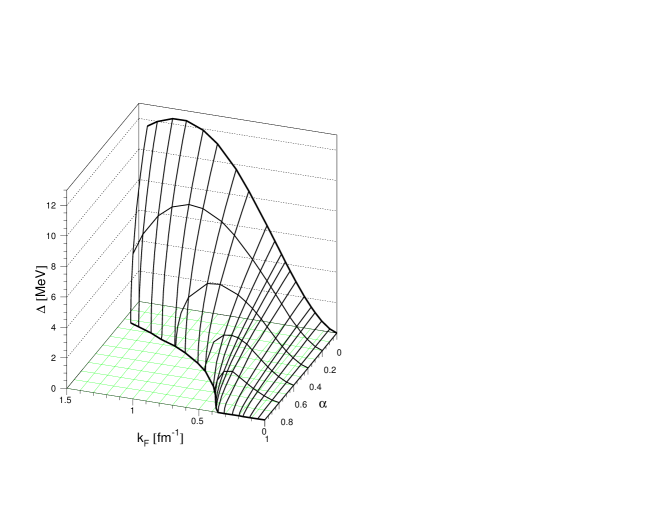
FIG. 4.: The pairing gap as a function of total density [$k_{F}\equiv(3\pi^{2}\rho/2)^{1/3}$] and asymmetry.

FIG. 5.: Proton momentum distributions $n_{p}(k)$, gap functions $\Delta(k)$, and anomalous densities $\psi(k)$, for different total densities $\rho=10^{-4},10^{-2},10^{-1}\;\rm fm^{-3}$, and different asymmetries. The dots indicate the boundaries of the interval containing the neutron excess in each case.

FIG. 6.: Top panel: The ${}^{3}SD_{1}$ gap in symmetric nuclear matter as a function of total density $\rho$ or equivalent Fermi momentum $k_{F}=(3\pi^{2}\rho/2)^{1/3}$ (solid line). The dashed line shows the analytical approximation Eq. (50). Central panel: The maximum asymmetry at which a gap exists (solid line) and the approximation Eq. (44) (dashed line). Lower panel: The values of the various chemical potentials $\mu,\delta\mu,\mu_{n},\mu_{p}$, corresponding to the asymmetry $\alpha_{\rm max}$ displayed in the panel above.

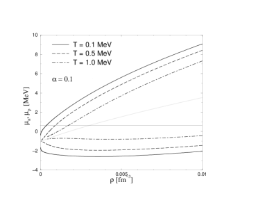
FIG. 7.: Chemical potentials of neutrons (upper curves) and protons (lower curves) at $\alpha=0.1$ as functions of density for different temperatures.

REFERENCES

• [1] A. J. Leggett, in Modern Trends in the Theory of Condensed Matter (Springer, Berlin, 1980), p.13; J. Phys. (Paris) 41, C7-19 (1980).
• [2] L. V. Keldysh and Yu. V. Kopaev, Sov. Phys. Solid State 6, 2219 (1965); L. V. Keldysh and A. N. Kozlov, Sov. Phys. JETP 27, 521 (1968).
• [3] P. Nozières and S. Schmitt-Rink, J. Low Temp. Phys. 59, 195 (1985).
• [4] T. Alm, B. L. Friman, G. Röpke, and H. Schulz, Nucl. Phys. A551, 45 (1993).
• [5] H. Stein, A. Schnell, T. Alm, and G. Röpke, Z. Phys. A351, 295 (1995).
• [6] M. Baldo, U. Lombardo, and P. Schuck, Phys. Rev. C52, 975 (1995).
• [7] A. Sedrakian, T. Alm, and U. Lombardo, Phys. Rev. C55, R582 (1997).
• [8] A. Sedrakian and U. Lombardo, Phys. Rev. Lett. 84, 602 (2000).
• [9] P. Ring and P. Schuck, The Nuclear Many-Body Problem (Springer, Berlin, 1980).
• [10] A. A. Abrikosov, L. P. Gorkov, and I. E. Dzyaloshinskii, Methods of Quantum Field Theory in Statistical Physics (Prentice-Hall, Englewood Cliffs, 1963).
• [11] P. Nozières, Le problème à N corps (Dunod, Paris, 1963).
• [12] P. Nozières, Theory of Interacting Fermi Systems (Benjamin, New York, 1966).
• [13] J. R. Schrieffer, Theory of Superconductivity (Addison-Wesley, New York, 1964).
• [14] A. B. Migdal, Theory of Finite Systems and Applications to Atomic Nuclei (Benjamin, New York, 1964).
• [15] D. R. Tilley and J. Tilley, Superfluidity and Superconductivity (IOP Publishing, Bristol, 1990).
• [16] M. Baldo, I. Bombaci, and U. Lombardo, Phys. Lett. B283, 8 (1992).
• [17] R. B. Wiringa, R. A. Smith, and T. L. Ainsworth, Phys. Rev. C29, 1207 (1984).
• [18] A. L. Goodman, Nucl. Phys. A186, 475 (1972); Phys. Rev. C60, 014311 (1999); Phys. Rev. C63, 044325 (2001).
• [19] U. Lombardo, H.-J. Schulze, and W. Zuo, Phys. Rev. C59, 2927 (1999);
E. Garrido, P. Sarriguren, E. Moya de Guerra, U. Lombardo, P. Schuck, and H.-J. Schulze, Phys. Rev. C63, 037304 (2001).
• [20] P. Bozek, Nucl. Phys. A657, 187 (1999); Phys. Rev. C62, 054316 (2000);
M. Baldo and A. Grasso, Phys. Lett. B485, 115 (2000);
U. Lombardo, P. Schuck, and W. Zuo, Phys. Rev. C, (September 2001).
• [21] A. L. Fetter and J. D. Walecka, Quantum Theory of Many-Particle Systems (McGraw-Hill, New-York, 1971).
• [22] H. T. C. Stoof, M. Houbiers, C. A. Sackett, and R. G. Hulet, Phys. Rev. Lett. 76, 10 (1996); M. Houbiers, R. Ferwerda, H. T. C. Stoof, W. I. McAlexander, C. A. Sackett, and R. G. Hulet, Phys. Rev. A56, 4864 (1997).
• [23] S. A. Fayans and D. Zawischa, in Recent Progress in Many-Body Theories, R. F. Bishop, K. A. Gernoth, N. R. Walet, and Y. Xia (eds.), 403 (World Scientific, Singapore, 2000).
Refer to caption