Nucleons and Isobars at finite density ($\rho$) and temperature ($T$)

Abstract

The importance of studying matter at high $\rho$ increases as more astrophysical data becomes available from recently launched spacecrafts. The importance of high $T$ studies derives from heavy ion data. In this paper we set up a formalism to study the nucleons and isobars with long and short range potentials non-pertubatively, bosonizing and expanding semi-classically the Feyman integrals up to one loop. We address the low density, finite T problem first, the case relevant to heavy ion collisions, hoping to adresss the high density case later. Interactions change the nucleon and isobar numbers at different $\rho$ and $T$ non-trivially.

¹⁾I.N.F.N., Sezione di Genova and Dipartimento di Fisica, Università di Genova, via Dodecaneso, 33-16146 Genova, Italy
²⁾Abdus Salam ICTP, Trieste, Italy and Azad Physics Centre,
Dept. of Physics, Maulana Azad College, Calcutta 700 013, India
³⁾Department of Physics, Presidency College, Calcutta 700 073,India; an associate member of Abdus Salam International Centre of Theoretical physics, Trieste, Italy ^† All communications to cenni@ge.infn.it and deyjm@giascl01.vsnl.net.it

1 Introduction

Isobars ($\Delta$’s) play a very important role in nuclear physics. Two pion exchange with a $\Delta$ intermediate state is known to produce the intermediate range attraction between nucleons[1]. Many attempts have been made to extract the effect of $\Delta$ intermediate states in nuclear matter dynamics, and microscopical calculations have shown the overwhelming relevance they have in binding of nuclear matter [1, 2].

$\Delta$ is the next excited state in the nucleon spectroscopy with a large degeneracy factor ( $4\times 4$ for spin and isospin). Paradoxically however not too much efforts have been devoted to extract the amount of $\Delta$ population in the nuclear matter ground state [3, 4]. It is on the other hand conceivable that the small numbers found so far (Ref. [3] clearly overestimates the $\Delta$ component of the nuclear ground state) suggest that the presence of $\Delta$’s could at most induce rather small effects in the ground state properties. Only recently use of modern $N$-$N$ interaction has renewed the interest in this field [5], but still dynamical aspects like spectral functions and response functions deserve further investigations even taking advantage of the modern computing facilities.

Even disregarding, however, the relevance of traditional nuclear matter calculations, new achievements both on the astrophysical sector and on the side of ultra-relativistic heavy-ions collisions suggest to explore the properties of the hadron matter at finite (high) temperature. One should keep in mind in fact that in the latter case a low density hadronic matter is expected to be the relic of a phase transition to and from a quark-gluon plasma phase. The knowledge of the nuclear matter properties at low density and high temperature is thus linked (maybe not in a simple way) to the signals that such a phase transition has indeed occurred. But such conditions seem to be much more sensitive to the presence of $\Delta$’s, as real $\Delta$’s can be produced.

This has already been established by calculations where non-interacting nucleon and isobar excited states are embedded in a thermal bath ( see for example Bebie et al. [6] and Dey et al. [7]). Interactions between nucleons ($N$ in short) and $\Delta$’s being strong, it is very difficult to handle. A non-perturbative treatment is mandatory.

The framework we use in this paper to deal with a system of interacting nucleons and isobars is provided by the path integral technique developed by one of us and his co-workers [8, 9, 10, 11]. It involves Bosonisation arising from integration over the fermionic fields.

For non-interacting fermions the methodology is simple. However, for long range one pion exchange potential ( OPEP ) or short range correlations (SRC in short) non-perturbative semi-classical approximation schemes are necessary. This provides a mean field. Higher order corrections can be put onto it.

The method is described in short in the next section. The nucleon and the isobar, being heavy particles can be treated non-relativistically. This allows the Fermi integrations and the Pauli principle to be dealt with. As the density , $\rho$, increases the baryons are packed more closely so that the Pauli principle is expected to play a crucial role.

2 The partition function for the Nucleon interacting with the Pion

To exemplify, we consider a system of nucleons interacting with pions. OPEP potential between nucleons and pions is written as

$$V_{\pi}({\bf q})=\Gamma_{i}^{(1)}{\cal V}_{\pi}({\bf q})\Gamma_{i}^{(2)}$$ (1)

where

$${\cal V}_{\pi}({\bf q})=-\frac{f^{2}_{\pi NN}}{m_{\pi}^{2}}\frac{{\bf q}^{2}}{{\bf q}^{2}+m_{\pi}^{2}}$$ (2)

and

$$\Gamma_{i}^{(1)}={\mbox{\boldmath$\sigma$}}_{1}\cdot\hat{\bf q}\tau_{i}\;.$$ (3)

The partition function in the grand canonical ensemble, in terms of path integrals, reads

$$Z=e^{-\beta\Omega}={\rm Tr}e^{-\beta(H-\mu N)}=\int D[\psi^{\dagger}(x),\psi(x)]e^{-\int_{0}^{\beta}d\tau\left[H(\tau)-\mu N(\tau)\right]}$$ (4)

where $H\,,\mu\,$ and $N$ are the Hamiltonian , the chemical potential and the number operator respectively.

For non-interacting nucleons we can easily evaluate the partition function in terms of the Fourier transforms for the fields $\psi({\bf q},\omega_{n})$ :

$$Z_{0}=Z=\int D[\psi^{\dagger},\psi]e^{\sum_{n}\int d^{3}q\psi^{\dagger}(-{\bf q},-\omega_{n}){\cal G}^{-1}_{0}(q,\omega_{n})\psi({\bf q},\omega_{n})}$$ (5)

where ${\cal G}_{0}(q,\omega_{n})$ is the free Green’s function at finite temperature :

$${\cal G}_{0}(q,\omega_{n})=-\frac{1}{\frac{q^{2}}{2M}-\mu-i\omega_{n}}$$ (6)

with

$$\omega_{n}=\frac{(2n+1)\pi}{\beta}\;;$$ (7)

the functional integration becomes the determinant of the Green’s function.

To evaluate the partition function with OPEP interaction , eqn.(4), an approximation scheme of boson loop expansion is used. This scheme has been explained in details in the already quoted refs. [9, 10, 11]. Basically, functional integral over the fermion fields leaves an effective bosonic Lagrangian which in the zeroth order gives rise to a mean field like that of RPA and in the 1st order to the one boson loop approximation.

This is achieved by availing of the Hubbard-Stratonovitch transformation [12, 13, 14] to convert the potential part inside the Feynman integrals into a functional integral. For example, the potential inside eqn.(4), under the Hubbard-Stratonovitch transformation, becomes

$$e^{-{i\over 2}\int_{0}^{\beta}\int d^{3}x\,d^{3}y\,\psi^{\dagger}(x)\Gamma_{i}\psi(x){\cal V}_{\pi}(|{\mbox{\boldmath$\scriptstyle x$}}-{\mbox{\boldmath$\scriptstyle y$}}|)\psi^{\dagger}(y)\Gamma_{i}\psi(y)}=\sqrt{\det(-{\cal V}_{\pi})}$$

$$\int D[\sigma_{i}]e^{{i\over 2}\int_{0}^{\beta}d\tau\int d^{3}x\,d^{3}y\sigma_{i}(x){\cal V}_{\pi}^{-1}(|{\mbox{\boldmath$\scriptstyle x$}}-{\mbox{\boldmath$\scriptstyle y$}}|)\sigma_{i}(y)+i\int_{0}^{\beta}d\tau\int d^{3}x\sigma_{i}(x)\psi^{\dagger}(x)\Gamma_{i}\psi(x)},$$

where the measure over $\sigma_{i}$ is defined as

$$D[\sigma_{i}(x)]\longrightarrow\prod_{k}\frac{d\sigma_{i}(x_{k})}{\sqrt{2\pi}}.$$

Performing the functional integration over the fermionic fields it becomes

$$Z=\sqrt{\det(-{\cal V}_{\pi})}\int D[\sigma_{i}]e^{\frac{1}{2}\sigma_{i}{\cal V}_{\pi}\sigma_{i}}\det\left[{\cal G}_{0}^{-1}-\sigma_{i}\Gamma_{i}\right]\;.$$ (9)

Since ${\cal G}_{0}^{-1}$ and $\sigma_{i}\Gamma_{i}$ commute :

$$Z=\sqrt{\det(-{\cal V}_{\pi})}\det{\cal G}_{0}^{-1}\int D[\sigma_{i}]e^{\frac{1}{2}\sigma_{i}{\cal V}_{\pi}\sigma_{i}+{\rm Tr}\log\left[I-{\cal G}_{0}\sigma_{i}\Gamma_{i}\right]}.$$ (10)

3 Introduction of $\Delta$’s, $\rho$-mesons and Short Range Correlations (SRC)

The simplest way to introduce the $\Delta$’s in this formalism is to generalise the nucleon field to a column vector

$$\psi=\left({\psi_{N}\atop\psi_{\Delta}}\right)$$ (11)

and the $\Gamma_{i}$ (eqn.3) as

$$\Gamma_{i}=\left(\matrix{{\mbox{\boldmath$\sigma$}}\cdot{\bf q}\tau_{i}&\frac{\displaystyle f_{\pi N\Delta}}{\displaystyle f_{\pi NN}}{\bf S}\cdot{\bf q}T_{i}\cr\frac{\displaystyle f_{\pi N\Delta}}{\displaystyle f_{\pi NN}}{\bf S}^{\dagger}\cdot{\bf q}T_{i}^{\dagger}&\frac{\displaystyle f_{\pi\Delta\Delta}}{\displaystyle f_{\pi NN}}{\mbox{\boldmath$\cal S$}}\cdot{\bf q}{\cal T}_{i}}\right)\;.$$ (12)

Free ${\cal G}^{0}_{\Delta}$ becomes

$${\cal G}^{0}_{\Delta}({\bf q},\omega_{n})=-\frac{1}{\frac{q^{2}}{2M_{\Delta}}+\delta M-\mu_{\Delta}-i\omega_{n}}$$ (13)

where $\delta M=M_{\Delta}-M$. Matrices ${\cal S}_{i}$ and ${\cal T}_{i}$ are the generators of the 3/2 representation of the $SU(2)$ group ( see for instance [11]). But $S_{i}$ and $T_{i}$ are the familiar 4 x 2 transition spin - isospin operators (see for example, [15]).

Further, a reasonable description of the dynamics of a nuclear system interacting via meson exchange needs to account, in order to be realistic, of short range correlations (SRC). This SRC has been introduced in nuclear systems in many ways, for example through the Landau-Migdal parameter $g^{\prime}$. It has been shown by [11] that at the one boson loop level, beyond the Landau-Migdal theory, a momentum dependence of $g^{\prime}$ is necessary. Now there are two independent parameters, namely the value of the function $g^{\prime}(q)$ at the origin and a cut-off that kills the effective interaction due to nucleon-nucleon (or nucleon-$\Delta$) short range repulsion. Both parameters are density dependent, in a way which is not known.

A simpler treatment to deal with SRC is given by Brown et al. [16] which is successfully applied by Oset and coworkers (see, among many other papers, [17]). It amounts to multiply the nucleon-nucleon interaction ${\cal V}(r)$ by the two-body correlation function $g(r)$, i.e.,

$${\cal V}(r)\longrightarrow g(r){\cal V}(r)\;,$$ (14)

and further to approximate $g(r)$ with

$$g(r)\simeq\frac{1}{3}j_{0}(q_{c}r)$$ (15)

where $q_{c}$ is taken roughly equal to the $\omega$-mass. This approach not only works well but also is almost parameter free. Density dependence of the correlations is automatically taken care of. It is to be noted that, it amounts to fix $g^{\prime}$ at about 0.7.

Of course a $\Delta$-hole pair can be excited by a $\rho$-meson as well. We shall see in the following that a $\rho$-meson exchange, with the same scheme for SRC as before, can also be included in the formalism. In the following calculations, $q_{c}^{\pi}=770$ MeV/c and $q_{c}^{\rho}=1200$ MeV/c.

4 The Loop Expansion

We now expand the partition function (eq.10) semi-classically. At the saddle point,i.e., at the mean field level, $\sigma_{i}\,=\,0$ and the partition function becomes

$$Z^{\rm mean~{}field}=\sqrt{\det-{\cal V}_{\pi}}\det{\cal G}_{0}^{-1}\;.$$ (16)

Quadratic deviations of the field from its mean field value lead to

$$\int D[\sigma_{i}]e^{\frac{1}{2}\sigma_{i}{\cal V}_{\pi}^{-1}\sigma_{i}-\frac{1}{2}{\rm Tr}\sigma_{i}\Gamma_{i}{\cal G}_{0}\sigma_{j}\Gamma_{j}{\cal G}_{0}}=\left\{\det{\cal V}_{\pi}^{-1}-{\rm Tr}\Gamma_{i}{\cal G}_{0}\Gamma_{j}{\cal G}_{0}\right\}^{-\frac{1}{2}}\;$$ (17)

so that the partition function (eq. 10) at the one loop order becomes

$$Z=\det{\cal G}_{0}^{-1}e^{Tr\log\left[I-{\cal V}_{\pi}\Gamma_{i}{\cal G}_{0}\Gamma_{j}{\cal G}_{0}\right]}=Z_{0}e^{{\rm Tr}\log\left[I-{\cal V}_{\pi}\Gamma_{i}{\cal G}_{0}\Gamma_{j}{\cal G}_{0}\right]}$$ (18)

where

$$Z_{0}=\prod_{q}\left(1+e^{-\beta\left[\frac{q^{2}}{2M}-\mu_{N}\right]}\right)\prod_{q}\left(1+e^{-\beta\left[\frac{q^{2}}{2M_{\Delta}}+\delta M-\mu_{\Delta}\right]}\right)\;.$$ (19)

The grand potential, $\Omega=-\frac{1}{\beta}\,logZ$, in one-loop order becomes

$$\Omega^{\rm 1-loop}=-\frac{1}{\beta}\left\{\log Z_{0}+{\rm Tr}\log\left[I-{\cal V}_{\pi}\Gamma_{i}{\cal G}_{0}\Gamma_{j}{\cal G}_{0}\right]\right\}$$ (20)

Thus for the 0-order part we get

$$\Omega_{0}=-\frac{V}{\beta}\int\frac{d^{3}q}{(2\pi)^{3}}\left\{\log\left[1+e^{-\beta\left(\frac{q^{2}}{2M}-\mu_{N}\right)}\right]+\log\left[1+e^{-\beta\left(\frac{q^{2}}{2M_{\Delta}}+\delta M-\mu_{\Delta}\right)}\right]\right\}$$ (21)

Derivatives of $\Omega$ with respect to $\mu_{N}$ and $\mu_{\Delta}$ result in $N$ and $\Delta$ numbers respectively. Therefore,

$$<N_{N}> = V\int\frac{d^{3}q}{(2\pi)^{3}}n_{N}^{0}(q)$$ (22)

$$<N_{\Delta}> = V\int\frac{d^{3}q}{(2\pi)^{3}}n_{\Delta}^{0}(q)$$ (23)

where

$$n_{N}^{0}(q) = \frac{1}{1+e^{\beta\left(\frac{q^{2}}{2M}-\mu_{N}\right)}}$$ (24)

$$n_{\Delta}^{0}(q) = \frac{1}{1+e^{\beta\left(\frac{q^{2}}{2M_{\Delta}}+\delta M-\mu_{\Delta}\right)}}\;.$$ (25)

For first order correction we define

$$\Pi^{0}=\frac{1}{q^{2}}{\rm Tr}\Gamma_{i}{\cal G}_{0}\Gamma_{i}{\cal G}_{0}$$ (26)

(the trace makes $i\not=j$ vanishing) which turns out to be the generalisation of the Lindhard function to the finite temperature case. We have three different $\Pi^{0}\,-s$, corresponding to the N particle - N hole, the $\Delta$ particle - N hole and the $\Delta$ particle -$\Delta$ hole propagators. The last one vanishes at the $T\to 0$ limit.

$$\Pi^{0}_{NN}({\bf q},\nu_{n}) = 4\int\frac{d^{3}k}{(2\pi)^{3}}\frac{n^{0}_{N}(k)-n^{0}_{N}(q+k)}{i\nu_{n}+\epsilon(k)-\epsilon(q+k)}$$ (27)

$$\Pi^{0}_{N\Delta}({\bf q},\nu_{n}) = \frac{16}{9}\int\frac{d^{3}k}{(2\pi)^{3}}\frac{n^{0}_{N}(k)-n^{0}_{\Delta}(q+k)}{i\nu_{n}+\epsilon(k)-\epsilon_{\Delta}(q+k)+\mu_{\Delta}-\mu_{N}}$$ (28)

$$+ (N\leftrightarrow\Delta)$$

$$\Pi^{0}_{\Delta\Delta}({\bf q},\nu_{n}) = 16\int\frac{d^{3}k}{(2\pi)^{3}}\frac{n^{0}_{\Delta}(k)-n^{0}_{\Delta}(q+k)}{i\nu_{n}+\epsilon_{\Delta}(k)-\epsilon_{\Delta}(q+k)}$$ (29)

where the numbers in front are contributions from the spin-isospin traces and

$$\nu_{n}=\frac{2n\pi}{\beta}\;.$$ (30)

The parity of these function with respect to $\nu_{n}$ simplify them further.

Thus the total $\Pi$ is given by

$$\Pi=f_{\pi NN}^{2}\Pi^{0}_{NN}+f_{\pi N\Delta}^{2}\Pi^{0}_{N\Delta}+f_{\pi\Delta\Delta}^{2}\Pi^{0}_{\Delta\Delta}\;.$$ (31)

so that one loop grand potential (eq.20) is

$$\Omega^{\rm 1-loop}=\Omega_{0}-\frac{1}{\beta}{\rm Tr}\log\left[I+{\cal V}_{\pi}q^{2}\Pi\right]=\Omega_{0}+\frac{1}{\beta}\sum_{n=1}^{\infty}\frac{1}{n}{\rm Tr}\left[{\cal V}_{\pi}\Pi\right]^{n}$$ (32)

Using the identity $\frac{1}{n}=\int\limits_{0}^{1}\lambda^{n-1}d\lambda$ and substituting ${\cal V}_{\pi}^{\lambda}=\lambda{\cal V}_{\pi}$ we get

$$\Omega^{\rm 1-loop}=\Omega_{0}+\frac{1}{\beta}\sum_{n=1}^{\infty}\int\limits_{0}^{1}\frac{d\lambda}{\lambda}{\rm Tr}\left[{\cal V}_{\pi}^{\lambda}\Pi\right]^{n}\,.$$ (33)

Further, summation of the series results in

$$\Omega^{\rm 1-loop}=\Omega_{0}+\frac{1}{\beta}\int\limits_{0}^{1}\frac{d\lambda}{\lambda}{\rm Tr}\frac{{\cal V}_{\pi}^{\lambda}\Pi}{1-{\cal V}_{\pi}^{\lambda}\Pi}\,.$$ (34)

The remaining trace means integration over the 3-momentum and sum over the frequencies.

Number of $\Delta$’s and nucleons can now be obtained easily.

$$<N_{\Delta}>=<N_{\Delta}>^{0}-\frac{1}{\beta}{\rm Tr}{{\cal V}_{\pi}\over 1-{\cal V}_{\pi}\Pi}\frac{\partial\Pi}{\partial\mu_{\Delta}}$$ (35)

and

$$<N_{N}>=<N_{N}>^{0}-\frac{1}{\beta}{\rm Tr}{{\cal V}_{\pi}\over 1-{\cal V}_{\pi}\Pi}\frac{\partial\Pi}{\partial\mu_{N}}$$ (36)

The 0-order quantities are given by (22) and (23). To evaluate eqs.(35) and (36) we find that 1st-order correction term (n=1 of eq.(32))

$$<N_{N}>^{\rm 1st-ord}=-\frac{1}{\beta}{\rm Tr}\frac{\partial~{}}{\partial\mu_{N}}\left[{\cal V}_{\pi}\Pi\right]\;$$

needs added attention because it is ill defined as in the case of self-energy of the nucleon in a medium :

$$\Sigma(k,\omega_{n})=\frac{1}{\beta}\sum_{n^{\prime}}\int\frac{d^{3}q}{(2\pi)^{3}}{\cal G}_{0}({\bf q},\omega_{n^{\prime}}){\cal V}_{\pi}(|{\bf k-q}|).$$ (37)

We need a convergence factor $e^{i\omega_{n^{\prime}}\eta}$ which produces an extra factor $n^{0}_{N}(q)$. The derivative with respect to $\mu_{N}$ gives

$$<N_{N}>^{\rm 1st-ord}=$$

$$12\int\frac{d^{3}q}{(2\pi)^{3}}\int\frac{d^{3}k}{(2\pi)^{3}}{\cal V}_{\pi}(|{\bf k-q}|)\frac{\partial~{}}{\partial\mu_{N}}\left[n_{N}^{0}(q)n_{N}^{0}(k)\right]$$

$$+\frac{16}{3}\int\frac{d^{3}q}{(2\pi)^{3}}\int\frac{d^{3}k}{(2\pi)^{3}}\frac{\partial~{}}{\partial\mu_{N}}\left[n_{N}^{0}(q)n_{\Delta}(k)+n_{N}^{0}(k)n_{\Delta}(q)\right]{\cal V}_{\pi}(|{\bf k-q}|)$$

Similarly one gets for the $\Delta$ contribution

$$<N_{\Delta}^{\rm 1st-ord}>=$$

$$\frac{16}{3}\int\frac{d^{3}q}{(2\pi)^{3}}\int\frac{d^{3}k}{(2\pi)^{3}}\frac{\partial~{}}{\partial\mu_{N}}\left[n_{N}^{0}(q)n_{\Delta}(k)+n_{N}^{0}(k)n_{\Delta}(q)\right]{\cal V}_{\pi}(|{\bf k-q}|)$$

$$+48\int\frac{d^{3}q}{(2\pi)^{3}}\int\frac{d^{3}k}{(2\pi)^{3}}{\cal V}_{\pi}(|{\bf k-q}|)\frac{\partial~{}}{\partial\mu_{N}}\left[n_{\Delta}(q)n_{\Delta}(k)\right]$$

The remaining part of the series can be evaluated straightforwardly :

$$-\frac{3}{\beta}\sum_{n}\int\frac{d^{3}q}{(2\pi)^{3}}\frac{{\cal V}_{\pi}^{2}\Pi}{1-{\cal V}_{\pi}\Pi}\frac{\partial\Pi}{\partial\mu_{N,\Delta}}\;.$$ (40)

by evaluating $\Pi^{0}$ -s (eqs. (27-29).

Some remarks are not out of place here.

1. Sum in eqn. (40) can be further transformed into an integral over the imaginary axis. But this does not make numerical calculation easier.

2. the present formalism amounts to evaluate the diagram of fig. 1

   

   Figure 1: One-loop diagram for the number of $\Delta$ and nucleons.

   where the black dot denotes the $\partial\Pi/\partial\mu$ insertion and the dashed circle the RPA-dressed pion. Since pions are spin-longitudinal while the $\rho$’s are spin-transverse and in an infinite medium $\Pi$ conserves the elicity, the two kinds of mesons cannot mix together. Thus the $\rho$ meson contribution simply amounts to the similar diagram with the pion exchange potential replaced by the $\rho$ exchange with a factor 2 in front of $\Pi$ coming from spin traces.

3. In general, $\partial\Pi\over\partial\mu$ in eqn. (40) obtained from eqns. (26-30) becomes ill-defined for $n=0$. But if eqns. (26-30) describe analytical functions, even for $n=0$, the singularity can be separated from the integral and handled analytically.

5 Numerical results: densities and chemical potential

The previous section provided the tool needed for the evaluation of $<N_{N}>$ and $<N_{\Delta}>$. At the equilibrium $\mu_{N}=\mu_{\Delta}=\mu$ and hence both $<N_{N}>$ and $<N_{\Delta}>$ can be regarded as functions of $\mu$. Putting for short $<N_{N}>=N_{N}(\mu)$ and $<N_{\Delta}>=N_{\Delta}(\mu)$ it is also clear that

$$N_{N}(\mu)+N_{\Delta}(\mu)=A=V\rho=V\frac{2k_{F}^{3}}{3\pi^{2}}\;,$$ (41)

where $A$ is the baryon number and the last equality can be regarded as a definition of an effective Fermi momentum. Here $\mu$ is the input of the problem. If instead we choose $A$ in order to fix the thermodynamical conditions of the system we need to consider (41) as an equation for $\mu$ and solve it numerically.

Fig. 2 displays the results of such a calculation. It shows the behaviour of the chemical potential at the equilibrium for different values of the temperature and the nuclear density. The graph contains only pion exchange at three different levels of complexity, namely calculations up to second order (dashed lines), full one-loop calculation (solid line) and full calculation with dynamical pion (dotted line). We remember that in the frame of Matsubara Green’s function the pion propagator reads

$$\Delta_{\pi}={1\over\omega_{n}^{2}+{\bf q}^{2}+m_{\pi}^{2}}\;.$$

The figure displays five bunches of lines, corresponding to five different densities, namely (starting from the above), $\rho/\rho_{0}$ = 0.2, 0.4, 0.6, 0.8, 1; of course $\rho_{0}$ denotes the normal nuclear density. Remarkably these three different dynamics are almost completely superimposed: only looking very carefully at the figure one sees that the dashed line is a little bit higher than the other two, that instead are practically coincident.

Figure 2: Chemical potential of a system of nucleons and $\Delta$’s interacting via pion exchange as a function of the temperature. Lines as explained in the text.

The second plot we present (fig. 3) displays instead the ratio between nucleon and $\Delta$ density keeping fixed the sum $\rho_{N}+\rho_{\Delta}=\rho$ again as a function of the temperature and with five bunches as before. Of course this time the highest bunch corresponds to the highest density.

Figure 3: Ratio $\rho_{\Delta}/\rho_{N}$ as a function of the temperature. Lines as above. The total densities are 0.2 $\rho_{0}$, 0.4 $\rho_{0}$, 0.6 $\rho_{0}$, 0.8 $\rho_{0}$ and 1 $\rho_{0}$ in ascending order. Only pions are accounted for.

Here the plots are much more sensitive to the dynamics.

Insofar we have only considered exchange of pions. Let us add some more dynamics by including the exchange of correlated $\rho$-mesons the results are shown in figs. 4 and 5.

Figure 4: Chemical potential of a system of nucleons and $\Delta$’s interacting via pion plus $\rho$ as a function of the temperature. Lines as explained in the text.

Figure 5: Ratio $\rho_{\Delta}/\rho_{N}$ as a function of the temperature, with pion plus $\rho$ exchange. Lines as in 4

Remarkably, the $\rho$-meson exchange lowers significantly the chemical potential, while the ratio $\rho_{\Delta}/\rho_{N}$ as a function of the temperature is sensible to it only in the low $T$ region, where the full dynamical calculation shows a remarkable reduction of the $\rho_{\Delta}/\rho_{N}$ ratio. At higher $T$ instead the effect fades out.

The model at hand contains only a few number of parameters. Coupling constants and cut-off are more or less well defined (we use here standard coupling $C_{\rho}=2.3$) the only crucial parameter being the one connected to SRC, and in particular $q_{c}^{\pi}$. Thus in figs. 6 and 7 we plot again the temperature and the ratio $\rho_{\Delta}/\rho_{N}$ for the most complete dynamical case ($\pi$ plus $\rho$ fully dynamic at the one-loop order but with different values of $q_{c}^{\pi}$, namely $q_{c}^{\pi}=650$ MeV/c, (solid line), $q_{c}^{\pi}=770$ MeV/c (dashed line) and $q_{c}^{\pi}=900$ MeV/c (dotted line); the same conventions as in the two previous figures are adopted.

Figure 6: Chemical potential of a system of nucleons and $\Delta$’s interacting via pion plus $\rho$ as a function of the temperature. Lines as explained in the text.

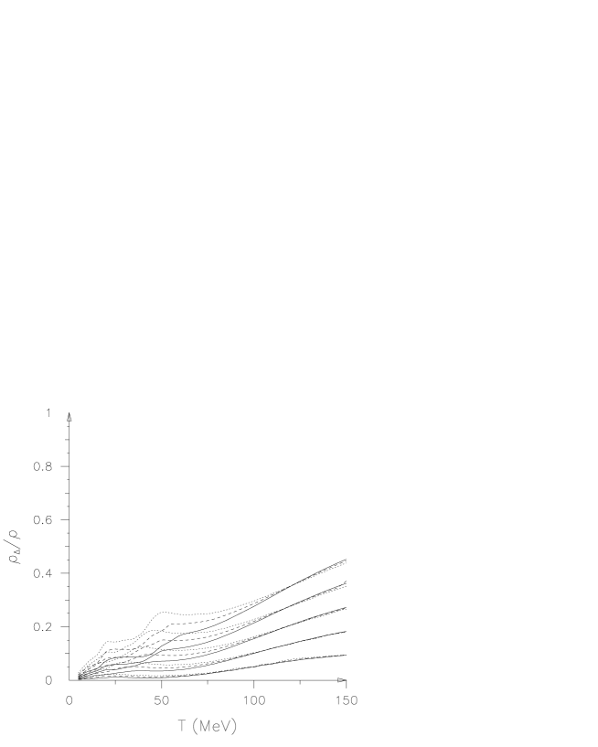
Figure 7: Ratio $\rho_{\Delta}/\rho_{N}$ as a function of the temperature, with pion plus $\rho$ exchange. Lines as in 6

We observe that while the chemical potential is almost insensitive to the variations of $q_{c}^{\pi}$ the ratio $\rho_{\Delta}/\rho_{N}$, on the contrary, shows that this ratio sensibly increases with $q_{c}^{\pi}$, in particular in an intermediate range of the temperature, while at temperatures of the order of 150 MeV the effect seems to fade out.

6 Numerical results: the momentum distribution

The momentum distribution displays an impressive dependence upon the temperature. We define the momentum distribution through the expression

$$<N>_{N} = {\rm Tr}\int\frac{d^{3}q}{(2\pi)^{3}}n_{N}(q)$$ (42)

$$<N>_{\Delta} = {\rm Tr}\int\frac{d^{3}q}{(2\pi)^{3}}n_{\Delta}(q)$$ (43)

the trace being taken over spin-isospin degrees of freedom (4 for nucleons, 16 for $\Delta$’s). In practice this amounts to take the integrand of all the previous calculations. Thus the result is a byproduct of the previous calculation. The results are plotted in fig. 8 for different temperatures and densities. The normalisation is everywhere to a $\theta(k_{F}-q)$ when $T\to 0$.

Figure 8: Momentum distribution of nucleons (solid line) and $\Delta$’s (dashed line) at different densities and temperatures

It is impressive to remark that the distribution is immediately spreaded to high momenta with the increasing of the temperature. Remind that the distribution is weighted with a $q^{2}$ in the Jacobian, so that the high momentum component become more and more important. An even more striking insight can be obtained by plotting the quantity $q^{2}n(q)$ and by comparing it with the Free Fermi Gas result at 0 temperature, as we do in fig 9. There it is clear that the areas of the curves is preserved while the shape is enormously modified.

Figure 9: Momentum distribution multiplied by $q^{2}$ of nucleons (solid line) and $\Delta$’s (dashed line) at different densities and temperatures. The dotted line corresponds to the Free Fermi Gas at 0 temperature.

Furthermore, at high temperature the dependence upon the density seems to become weak and something like an universal behaviour could be suggested.

7 Discussions

People speculate about the number of isobars in a hot soup of hadrons produced in a heavy ion collision. Even assuming that the short time available in heavy ion collisions is enough to thermalize the baryons and produce a uniform collective flow, the dynamics discussed in this paper is not sufficient to enlight the great variety of processes that could occur at finite temperature.

The vacuum at finite temperature is known to contain pions, since these particles are light. Dey et al [18] have shown that finite temperature will couple channels with different parity and isotopic spin. For example the $\rho$ and the $A_{1}$ meson along with a longitudinal pion mix to order $T^{2}$. The poles do not move till the next order $T^{4}$. In the same way the nucleon at finite $T$ will couple to the $\Delta_{1/2}$ state and the isobar to the nucleon excited state, $N^{*}_{3/2}(1520)$ as well as the odd parity isobar $\Delta(1700)$ [19].

Further, if we focus on the relic of a previously realized quark-gluon condesate, then the strangeness contribution should be relevant, and investigations on strange hyperons is also suggested [20].

Coming to more conventional degrees of freedom, it was shown by Bedaque [21] in a long letter, using chiral perturbation theory, that the nucleon mass increases a little, but that the nucleon acquires a substantial width and the mass is decreased so that the isobar-nucleon splitting becomes smaller. In chiral limit Bedaque’s result would appear in order $T^{4}$.

The present considerations seem thus suggest as future perspectives the extension of the present 1-loop calculation by one side to the study of other observables in a hadron gas, like for instance effective masses and widths and also the entropy of the system; and on the other side to the extension of the present scheme to a richer dynamics encompassing vector mesons and strange hadrons.

A further interesting development, to be carried out in the future, will be to extract, from the present formalism, the corresponding behaviour as an expansion in powers of the temperature.

Aknowledgements

J.D. and M.D. acknowledge hospitality at Abdus Salam ICTP and a D.S.T. research grant no. SP/S2/K18/96, Govt. of India for partial support. M.D. acknowledges the kind hospitality at the Dipartimento di Fisica, Università di Genova, Genova.

References

• [1] R. Machleidt, K. Holinde and Ch. Elster.  . Phys. Rep., C149:1, 1987.
• [2] R. Cenni, F. Conte and G. Dillon.  . Nuovo Cimento Lett., 43:39, 1985.
• [3] M. R. Anastasio et al.  . Nucl. Phys., A322:369, 1979.
• [4] R. Cenni, F. Conte and U. Lorenzini.  . Phys. Rev., C39:1588, 1989.
• [5] T. Frick, S. Kaiser, H. Müther and A. Polls. nucl-th/0101028 preprint.
• [6] H. Bebie, P. Gerber, J. L. Goity and H. Leutwyler.  . Nucl. Phys., B378:95, 1992.
• [7] J. Dey, G. Krein, L. Tomio and T. Frederico.  . Z. Phys., C64:965, 1994.
• [8] W. M. Alberico, R. Cenni, A. Molinari and P. Saracco.  . Ann. of Phys., 174:131, 1987.
• [9] W. M. Alberico, R. Cenni, A. Molinari and P. Saracco.  . Phys. Rev., C38:2389, 1988.
• [10] R. Cenni and P. Saracco.  . Phys. Rev., C50:1851, 1994.
• [11] R. Cenni, F. Conte and P. Saracco.  . Nucl. Phys, A623:391, 1997.
• [12] G. Morandi, E. Galleani d’Agliano, F. Napoli and C. Ratto.  . Adv. Phys., 23:867, 1974.
• [13] H. Keiter.  . Phys. Rev., 2B:3777, 1970.
• [14] H. Kleinert.  . Fort. Phys., 26:565, 1978.
• [15] G. E. Brown and W. Weise.  . Phys. Rep., C22:281, 1975.
• [16] G. E. Brown, S. O. Bäckman, E. Oset and W. Weise.  . Nucl. Phys., A286:191, 1977.
• [17] R. C. Carrasco and E. Oset.  . Nucl. Phys., A536:445, 1992.
• [18] M. Dey, V. L. Eletsky and B. L. Ioffe.  . Phys. Lett., B252:620, 1990.
• [19] V. L. Eletsky and B. L. Ioffe.  . Phys. Rev., D47:3083, 1993.
• [20] E. L. Bratkovskaya et al.  . Nucl Phys., A681:84c, 2001.
• [21] P. F. Bedaque.  . Phys. Lett., B387:1, 1996.