Modeling the strangeness content of hadronic matter

Abstract

The strangeness content of hadronic matter is studied in a string-flip model that reproduces various aspects of the QCD-inspired phenomenology, such as quark clustering at low density and color deconfinement at high density, while avoiding long range van der Waals forces. Hadronic matter is modeled in terms of its quark constituents by taking into account its internal flavor (u,d,s) and color (red, blue, green) degrees of freedom. Variational Monte-Carlo simulations in three spatial dimensions are performed for the ground-state energy of the system. The onset of the transition to strange matter is found to be influenced by weak, yet not negligible, clustering correlations. The phase diagram of the system displays an interesting structure containing both continuous and discontinuous phase transitions. Strange matter is found to be absolutely stable in the model.

PACS 12.39.-x, 24.85.+p, 26.60.+c

I Introduction

Strange matter, a deconfined state of quark matter consisting of almost equal amounts of up, down, and strange quarks, has been speculated to be the absolute ground state of hadronic matter [1, 2]. If true, nucleons and nuclei — and thus most of the luminous matter in the universe — is in a long-lived metastable state. Undoubtedly, the confirmation of such hypothesis would have far reaching consequences on a variety of fields, ranging from astronomy and cosmology all the way to particle and nuclear physics. Stimulated by such an exciting possibility, searches for strange matter are currently being conducted at terrestrial laboratories as well as at space-based observatories. Indeed, a substantial effort has been devoted on experimental searches for strangelets (“strange-matter nuggets”) at both CERN and Brookhaven National Laboratory (BNL) and more are proposed in the future for the relativistic heavy-ion collider (RHIC) and the large-hadronic collider (LHC). These terrestrial experiments are being complemented by observational searches for strange stars. What would be the signature for such exotic objects? Since strange stars are self-bound objects having a mass-radius relation quite different than the gravitationally bound neutron stars, they are allowed rotational periods considerably shorter than those predicted for gravitationally bound stars. Consequently, if a pulsar with a period falling below the limit of gravitationally bound stars were discovered, the conclusion that the confined hadronic phase of nucleons and nuclei is only metastable would be virtually inescapable [3].

Such a pulsar may have been recently discovered [4, 5]. The pulsar SAX J1808.4-3658, with a rotation period of 2.5 ms, is the fastest spinning x-ray pulsar ever observed. Based on a study of its mass-radius relation it has been concluded that SAX J1808.4-3658 is a likely strange-star candidate [6], although this interpretation remains controversial [7, 8]. Still, the discovery of such a fastly-rotating pulsar appears to have made the detection of strange matter within observational reach. In turn, the confirmation of such an exotic state of matter will help settle the claim that at present our universe is in a long-lived metastable state.

In the present work we focus on the impact of strangeness on the equation of state (EOS). One motivation for this study, in addition to those mentioned earlier, is the observation that the masses of about 20 neutron stars are remarkably close to the “canonical” value of $M=1.4M_{\odot}$ [9]. Yet conventional models of nuclear structure, with equation of states constrained from the bulk properties of nuclear matter, seem to allow substantially larger masses [3, 10]. However, the existence of a quark-matter phase at the core of neutron stars (NS) will soften considerably the equation of state leading to smaller limiting masses. Thus a study of the strangeness content of hadronic matter, using a “QCD-inspired” model, is desirable. For static and spherically symmetric neutron stars obeying the Oppenheimer-Volkoff equations the only physical ingredient that remains to be specified is the equation of state. Yet an equation of state that is accurate over the whole range of densities present in a neutron star remains a formidable challenge. For example, such an equation of state should be able to describe the hypothetical “hybrid stars”: neutron stars consisting of a quark-matter core below a nuclear-matter mantle. Unfortunately, traditional studies of strange matter has been conducted in two vastly different pictures [11, 12, 13, 14]. One picture uses a hadronic model — similar to ordinary nuclei — where the fundamental degrees of freedom are mesons and baryons. The other picture uses a quark model consisting of massless, noninteracting quarks confined inside a bag. Presumably a description of strange matter in terms of mesons and baryons is well motivated in the low-density regime where clustering correlations remain important. At the same time, strange matter viewed as a relativistic Fermi gas of quark might be appropriate at the extremes of densities necessary for color deconfinement to occur. Yet this division seems ad-hoc and arbitrary; for example, at what density should one switch from a nuclear- to quark-based description? Perhaps the most serious difficulty encountered in modeling the density dependence of hadronic matter and the resulting EOS is how to model a system that has quarks confined inside color-neutral hadrons at low density but free quarks at high density. Much of the responsibility for such complexity rests on the self-interactions among the gluons which generate quark confinement in the low-density regime. On the other hand, the quark substructure of the hadrons should become important as the density increases.

Although the evidence in support of QCD as the correct theory of the strong interactions is overwhelming, at present no rigorous solution of QCD exists in the regime of high-baryon density. Thus, one must resort to QCD-inspired phenomenological models. Such models of hadronic matter using quarks as the underlying degrees of freedom have been developed to reproduce some properties of QCD [15, 16, 17, 18, 19]. The main feature of these models — generically known as “string-flip” models [20] — is the existence of a many-body potential able to confine quarks within color-singlet clusters without generating unphysical long-range van der Waals forces [21]. The many-body potential is evaluated by solving a difficult optimization problem; one must decide how to assign colored quarks into color-singlet clusters (see below). Presumably, this “quark-assignment” problem is meant to represent the optimal configuration of gluonic strings. While the precise form of the potential is presently unknown, the many-quark problem is likely to require solving some complicated global optimization problem. Although string-flip models violate important symmetries of QCD, such as chiral symmetry and Lorentz invariance, they excel in places where most other models fail: the transition from nuclear to quark-matter. In the string-flip moedl this transition is dynamical without the need to rely on ad-hoc parameters. Hence, such models should shed light on the possibility of stable strange matter. That the emergence of strange quarks at high-baryon density is energetically favorable is easy to understand. As the density of the system increases, the Pauli exclusion principle forces the chemical potential to increase from the light-quark mass $m$ to $E_{\rm F}=\sqrt{k_{\rm F}^{2}+m^{2}}$, where $k_{\rm F}$ is the Fermi momentum. What is not easy to understand are the details of the transition. For example, do clustering correlations remain important at the transition density or has the system evaporated into the free quarks? Does the EOS predicted by the model yield self-bound and absolutely stable strange stars? These are the sort of questions that we plan to address in this paper.

An initial study of strange matter in the string-flip model was carried out in Ref. [22]. There, a highly simplified version of the model was used to simulate one-dimensional matter in terms of two-color, two-flavor (“up” and “strange”) constituent quarks. While it was found that clustering correlations remain important in the transition region, strange matter was found to be unbound. In this paper we extend the results of Ref. [22] by simulating three-flavor (up, down, and strange), three-color (“red”, “blue”, and “green” ) hadronic matter in three-dimensional space. A variety of ground-state observables are computed as a function of density with the goal of characterizing the transition to strange matter and to establish the possibility of absolute stability. We have organized the paper as follows: Sec. II introduces the general ideas used to model a system of fermions focusing on the structure of the wave function and the many-body potential. We then consider both the low- and high-density limits to establish closed-form baseline results. After describing the variational Monte Carlo procedure, results are presented for a variety of ground-state observables. Finally, we offer conclusions and perspectives for future work in Sec. IV.

II Formalism

A The many-quark potential

The QCD-inspired phenomenology prescribes how to model the many-quark potential. At very-low density the quarks must be confined within color-singlet clusters that should interact weakly due to the short-range nature of the nucleon-nucleon interaction. This suggests a strong—indeed confining—force between quarks in the same cluster but no further interaction between quarks in different clusters. Thus, the force saturates within each color-singlet hadron. This saturatation is necessary in order for the hadrons to be able to separate without generating unphysical long-range forces. In contrast, in the high-density domain asymptotic freedom demands that the interaction between all quarks be weak. This behavior is expected once the average inter-quark separation becomes smaller than the typical confining scale. In this regime the only important correlation among quarks will be induced by the Pauli exclusion principle and the system should evolve into a Fermi gas of quarks.

A many-quark potential that meets these requirements was first introduced by Lenz and collaborators [20] to model meson-meson interactions. Soon after the potential was adapted by Horowitz, Moniz, and Negele for the study of one-dimensional nuclear matter [15]. Several more realistic generalizations have followed [16, 17, 18, 19], although all limited to non-strange matter. It is on one of these models [18] that we base our present generalization to strange matter. The model is constructed from quarks having flavor (up, down, strange) and color (red, blue, green) degrees of freedom. The many-quark potential is defined as the optimal clustering of quarks into color-singlet objects. For reasons that will become clear later, the implementation of this idea is carried out as follows. Consider all red and blue quarks in the system, irrespective of flavor in accordance to the “flavor-blind” nature of QCD. We define the “optimal pairing” of red and blue quarks as:

$$V_{RB}=\mathop{\min}_{P}\sum_{i=1}^{A}v\Big{(}{\bf r}_{iR},P({\bf r}_{iB})\Big{)}\;,$$ (1)

where ${\bf r}_{iR}$ denotes the spatial coordinate of the ith red quark and $P({\bf r}_{iB})$ is the coordinate of the mapped ith blue quark (${\bf r}_{iB}\mapsto P({\bf r}_{iB})\!\equiv\!{\bf r}_{jB}$). Note that the minimization procedure is over all possible $A!$ permutations of the $A$ blue quarks and that the confining potential $v$ is assumed harmonic with a spring constant denoted by $k$ (see Fig. 1). That is,

$$v({\bf r}_{iR},{\bf r}_{jB})=\frac{1}{2}k({\bf r}_{iR}-{\bf r}_{jB})^{2}\;.$$ (2)

The “blue-green” and “green-red” components of the many-quark potential are defined in direct analogy to Eq. (1)

$$V_{BG} = \mathop{\min}_{P}\sum_{i=1}^{A}v\Big{(}{\bf r}_{iB},P({\bf r}_{iG})\Big{)}\;,$$ (4)

$$V_{GR} = \mathop{\min}_{P}\sum_{i=1}^{A}v\Big{(}{\bf r}_{iG},P({\bf r}_{iR})\Big{)}\;.$$ (5)

In this manner the many-quark potential to be used in our simulations of strange matter becomes equal to:

$$V=V_{RB}+V_{BG}+V_{GR}$$ (6)

and thus, the Hamiltonian describing the system of $N$ particles each with mass $m_{i}$ and momentum ${\bf p}_{i}$ is given by:

$$H=\sum_{i=1}^{N}\frac{{\bf p}_{i}^{2}}{2m_{i}}+V\;.$$ (7)

Several comments are now in order. First, the constructed potential is able to confine quarks within color-singlet clusters. Yet the strong confining force saturates within each color-singlet cluster allowing the clusters to separate without generating long-range van der Waals forces. Moreover, the potential is symmetric under the exchange of identical quarks. Second, the potential is truly many-body as moving one single quark might cause many of the “strings” to flip; note that even those strings that are not connected to the moving quark might flip. Third, although at very low density quarks will overwhelmingly belong to three-quark clusters, there is no guarantee that this will remain true at higher densities; color-singlet clusters may also be formed from 6-, 9-, $\ldots$ 3A-quark configurations (see Fig. 1). Finally, the dynamically-induced residual interaction between color-singlet clusters will be generated exclusively through quark exchange, which induces a weak intermediate-range attraction between clusters, and the Pauli exclusion principle between quarks, which generates a strong short-range repulsion.

As discussed early in this section, the strict demands imposed by QCD on phenomenological models justifies the introduction of such a complex many-body potential. While its exact functional form remains uncertain, the requirements of quark confinement and cluster separability are likely to depend on solving some type of quark assignment problem. For simulations involving a large number of quarks an efficient clustering algorithm is of utmost importance. Indeed, finding the optimal clustering of $N=3A$ quarks into $A$ color-singlet objects requires searching among $(A!)^{2}$ configurations. Even for a modest system containing only $A\!=\!10$ hadrons the number of possible configurations already exceeds ten trillion! Clearly, a “brute-force” algorithm is impractical. Moreover, “three-dimensional stable matching problems”, such as the three-quark assignment problem, have been shown to be NP-complete [26]. Thus, an efficient algorithm is unlikely to exist. But for the version of the string-flip model adopted in this work—where the clustering of quarks within color-singlet objects is done pairwise—an efficient algorithm exists in the Hungarian method for the weighted bipartite matching problem which finds the optimal pairing in a time proportional to $A^{3}$ [25]. Note that while in this case the number of possible configurations grows“only” as $A!$, a brute-force algorithm remains impractical. Thus, without such an efficient algorithm our simulations would be limited to a very small number of quarks.

B The variational wave function

We are interested in describing the evolution of the system with baryon density. For that purpose we use a variational Monte-Carlo approach based on a one-parameter wave function of the form:

$$\Psi_{\lambda}(x)=e^{-\lambda V(x)}\Phi_{FG}(x)\;,$$ (8)

where $\lambda$ is the variational parameter, $V(x)$ is the many-body potential defined in Eq. (6), and $\Phi_{FG}(x)$ is the Fermi-gas wave function. This choice is motivated by QCD which dictates that at low density, when the average inter-quark separation is much larger than the confining scale, quarks should cluster into three-quark color-singlet hadrons. Thus, in the low-density regime the potential between quarks in the same hadron is strong but, as the interaction saturates within each cluster, the residual interaction between hadrons is very weak. Hence, the system resembles a Fermi gas of weakly interacting hadrons. It is the exponential term in the variational wave function that becomes responsible for inducing the clustering correlations. In contrast, in the high-density limit, characterized now by an average inter-quark separation much smaller than the confining scale, asymptotic freedom should take over. In this regime the interactions between quarks are weak and the system “dissolves” into a free Fermi gas of quarks. As will be shown below, the variational parameter evolves from a large (isolated-cluster) value at low density all the way to zero at high density, as the only remaining correlations between quarks are those induced by the Pauli exclusion principle.

1 Fermi-gas wave function

To describe a non-interacting system of quarks a Fermi-gas wave function, given in the form of a Slater determinant, is used for each color-flavor combination of quarks. Each of these Slater determinants is given by:

$$\Phi_{FG}(x)=\left|\matrix{\phi_{{\bf n}_{\hbox{\lower 0.64583pt\hbox{${\scriptscriptstyle 1}$}}}}({\bf x}_{1})&\phi_{{\bf n}_{\hbox{\lower 0.64583pt\hbox{${\scriptscriptstyle 1}$}}}}({\bf x}_{2})&\ldots&\phi_{{\bf n}_{\hbox{\lower 0.64583pt\hbox{${\scriptscriptstyle 1}$}}}}({\bf x}_{N})\cr\phi_{{\bf n}_{\hbox{\lower 0.64583pt\hbox{${\scriptscriptstyle 2}$}}}}({\bf x}_{1})&\phi_{{\bf n}_{\hbox{\lower 0.64583pt\hbox{${\scriptscriptstyle 2}$}}}}({\bf x}_{2})&\ldots&\phi_{{\bf n}_{\hbox{\lower 0.64583pt\hbox{${\scriptscriptstyle 2}$}}}}({\bf x}_{N})\cr\vdots&\vdots&\ddots&\vdots\cr\phi_{{\bf n}_{\hbox{\lower 0.64583pt\hbox{${\scriptscriptstyle N}$}}}}({\bf x}_{1})&\phi_{{\bf n}_{\hbox{\lower 0.64583pt\hbox{${\scriptscriptstyle N}$}}}}({\bf x}_{2})&\ldots&\phi_{{\bf n}_{\hbox{\lower 0.64583pt\hbox{${\scriptscriptstyle N}$}}}}({\bf x}_{N})}\right|\;.$$ (9)

where $\phi_{\bf n}({\bf x})$ represents a single-particle eigenstate for a free particle in a box with quantum numbers ${\bf n}$ (see below). This construction ensures that the wave function is totally antisymmetric under the exchange of identical quarks. To determine the single-particle wave functions we consider a single quark of mass $a$ confined to a three-dimensional box of side $a$ with antiperiodic boundary conditions. The energy of each single particle state is characterized by three integer quantum numbers ${\bf n}\!\equiv\!(n_{x},n_{y},n_{z})$:

$$E_{\bf n}=\frac{\pi^{2}}{2ma^{2}}(n_{x}^{2}+n_{y}^{2}+n_{z}^{2})\;,\quad(n_{i}=1,3,5,\ldots)\;.$$ (10)

Note that throughout this work we employ units in which $\hbar\!=\!c\!=\!1$. Each energy value, however, is at least eight-fold degenerate because there are even and odd solutions of the Schrödinger equation in each of the three spatial dimensions. Thus, a typical basis state is of the form:

$$\phi_{n_{x},n_{y},n_{z}}^{+,+,-}({\bf x})=\cos\left(\frac{n_{x}\pi}{a}x\right)\cos\left(\frac{n_{y}\pi}{a}y\right)\sin\left(\frac{n_{z}\pi}{a}z\right)\;.$$ (11)

In this way the system develops a “shell structure” with each shell holding, at least, eight quarks of each color-flavor combination. Let us illustrate how the shells are filled as the single-particle energy increases. Expressing the single-particle energies in units of ${\pi^{2}}/{2ma^{2}}$, the lowest shell has an energy of $3$ $(n_{x}\!=\!n_{y}\!=\!n_{z}\!=\!1)$ and is exactly eight-fold degenerate. The next shell, with an energy of $11$ ($n_{x}\!=\!n_{y}\!=\!1,n_{z}\!=\!3$ and permutations) holds 24 quarks, and so on (for more details see Table I).

2 Low-density limit

In the low-density regime quarks are confined within weakly-interacting color-singlet (red+blue+green=white) clusters. Further, although the model allows the existence of multi-quark configurations, the probability that color-singlet clusters with more than three quarks are formed is vanishingly small [18]. Finally, at these low densities the onset of strangeness is hindered by the large strange-quark mass. Thus, in this limit the variational wave function is exact, as we now show.

Consider a nucleon as a nonrelativistic system of three quarks of mass $m$ interacting via a confining potential assumed harmonic of spring constant $k$

$$H=\sum_{i=1}^{3}\frac{{\bf p}_{i}^{2}}{2m}+\sum_{i<j=1}^{3}\frac{1}{2}k({\bf r}_{i}-{\bf r}_{j})^{2}\;.$$ (12)

This is perhaps the simplest version of the surprisingly successful nonrelativistic quark model [23]. Introducing center-of-mass and two relative coordinates

$${\bf R}_{CM} = \frac{1}{3}({\bf r}_{1}+{\bf r}_{2}+{\bf r}_{3})\;,$$ (14)

$${\mbox{\boldmath$\xi$}_{1}} = \frac{1}{\sqrt{2}}({\bf r}_{1}-{\bf r}_{2})\;,$$ (15)

$${\mbox{\boldmath$\xi$}_{2}} = \frac{1}{\sqrt{6}}({\bf r}_{1}+{\bf r}_{2}-2{\bf r}_{3})\;,$$ (16)

enables one to rewrite the above Hamiltonian as a system of two uncoupled harmonic oscillators:

$$H=\frac{P_{CM}^{2}}{6m}+\left(\frac{P_{1}^{2}}{2m}+\frac{3}{2}k\xi_{1}^{2}\right)+\left(\frac{P_{2}^{2}}{2m}+\frac{3}{2}k\xi_{2}^{2}\right)\;.$$ (17)

The ground-state properties for the system are now easily inferred. For example, the energy per quark is given by

$$E_{0}/N-m=\omega=\sqrt{\frac{3k}{m}}\rightarrow\sqrt{3}\approx 1.732\;.$$ (18)

where the arrow in the above expression is meant to represent the value of the energy in units in which $k\!=\!m\!=\!1$; this system of units is adopted henceforth. Further, up to an overall normalization factor, the ground-state wave function is also easily computed; it is given by

$$\Psi_{0}({\mbox{\boldmath$\xi$}_{1}},{\mbox{\boldmath$\xi$}_{2}})=\exp\left(-\frac{\xi_{1}^{2}+\xi_{2}^{2}}{2b^{2}}\right)=\exp\left(-\frac{v({\mbox{\boldmath$\xi$}_{1}},{\mbox{\boldmath$\xi$}_{2}})}{3kb^{2}}\right)\;,$$ (19)

where the oscillator-length parameter $b\!\equiv\!(3km)^{-1/4}\!\rightarrow\!3^{-1/4}$ has been introduced. Note that we have used the fact that the above exponent is proportional to the potential energy of the baryon [see Eq. (17)] to write the second expression for the ground-state wave function. This expression suggests that in the limit of very low density the variational wave function defined in Eq. (8) becomes exact provided:

$$\lambda=\frac{1}{3kb^{2}}\longrightarrow\frac{1}{\sqrt{3}}\approx 0.577\;.$$ (20)

Note that in the low-density limit the Fermi-gas component of the wave function is not important, as the average separation between quarks of the same color-flavor combination is much larger than the “Pauli hole”.

3 High-density limit

The variational wave function is also exact in the limit of very high density. In this asymptotically-free regime the interaction between quarks is negligible so the only remaining correlations among them are those generated by the Pauli-exclusion principle. Thus, the system is described by a Fermi-gas wave function which represents the $\lambda\rightarrow 0$ limit of the variational wave function given in Eq. (8).

A Fermi-gas description is useful in establishing a baseline against which more sophisticated models may be compared. In addition, all observables that will be presented here can be computed analytically in the Fermi-gas limit. Hence let us start by computing the transition density to strange matter. This critical density is obtained by requiring that the chemical potential for the light ($u$ and $d$) quarks be identical to the strange-quark mass ($M$). That is,

$$m+\frac{k_{Fc}^{2}}{2m}=M\;\;{\rm or}\;\;k_{Fc}=\sqrt{2m(M-m)}\rightarrow 1.095\;.$$ (21)

Note that we have adopted a value of $M/m\!=\!1.6$ for the heavy-to-light mass ratio. Adopting a constituent light-quark mass of $m\!=\!300$ MeV, the transition density in physical units corresponds (with $N_{u}\!\equiv\!N_{d}$) to

$$k_{Fc}=328.634~{}{\rm MeV}\;\;{\rm or}\;\;\rho_{c}=\frac{k_{Fc}^{3}}{\pi^{2}}=0.468~{}{\rm fm}^{-3}\;.$$ (22)

Note that spin degrees of freedom, or spin-dependent interactions, have yet to be included in the model.

Let us proceed to evaluate the equation of state and the strangeness-to-baryon ratio as a function of density. First, however, we introduce the following definitions:

$$\rho=\frac{k_{F}^{3}}{\pi^{2}}\;\;{\rm and}\;\;\sigma=\frac{N_{s}}{N}=1-2\frac{N_{u}}{N}\;.$$ (23)

In terms of these relations the Fermi momenta become

$$k_{F}^{u}=(1-\sigma)^{1/3}k_{F}\;\;{\rm and}\;\;k_{F}^{s}=(2\sigma)^{1/3}k_{F}\;.$$ (24)

Moreover, the total energy-per-particle of the system — at fixed density ($\rho$) and strangeness-per-quark ($\sigma$) — may now be easily computed. We obtain

$$\frac{T_{FG}(\rho,\sigma)}{N}=(1-\sigma)m+\sigma M+\frac{3k_{F}^{2}}{10m}(1-\sigma)^{5/3}+\frac{3k_{F}^{2}}{20M}(2\sigma)^{5/3}\;.$$ (25)

The strangeness-per-quark is now determined by demanding that the total energy of the system be minimized at fixed density. That is,

$$\left(\frac{\partial T_{FG}/N}{\partial\sigma}\right)=\left[M+\frac{k_{F}^{2}}{2M}(2\sigma)^{2/3}\right]-\left[m+\frac{k_{F}^{2}}{2m}(1-\sigma)^{2/3}\right]=0\;.$$ (26)

This equation reflects the condition for chemical equilibrium: the chemical potential for both species of quarks (light and heavy) must be equal. In particular, at $\sigma\!\equiv\!0$, which corresponds to the onset of the transition to strange-quark matter, one recovers the critical density computed in Eq. (21).

Another useful observable to characterize the transition to quark matter is the two-body correlation function [24]

$$\rho{\hbox{\lower 3.0pt\hbox{${{}_{2}}$}}}({\bf r})=\sum_{\alpha\beta}\langle\Psi_{0}|\hat{\psi}_{\alpha}^{\dagger}({\bf r})\hat{\psi}_{\beta}^{\dagger}({\bf 0})\hat{\psi}_{\beta}({\bf 0})\hat{\psi}_{\alpha}({\bf r})|\Psi_{0}\rangle\;,$$ (27)

where $\alpha$ (and $\beta$) denotes the collection of all internal quantum numbers, such as color and flavor. The two-body correlation function measures the probability that two given quarks be separated by a distance ${\bf r}$. In the Fermi-gas limit, where the ground-state wave function may be written as a Slater determinant, the two-body correlation function may be readily evaluated. We obtain,

$$g{\hbox{\lower 3.0pt\hbox{${{}_{2}}$}}}({\bf r})\equiv\frac{\rho{\hbox{\lower 3.0pt\hbox{${{}_{2}}$}}}({\bf r})}{\rho^{2}}=1-\frac{1}{3}\left(\frac{3j_{1}(k_{F}r)}{k_{F}r}\right)^{2}\;,$$ (28)

where the spherical Bessel function is given by

$$j_{1}(x)=\left(\frac{\sin x}{x^{2}}-\frac{\cos x}{x}\right)\mathop{\longrightarrow}_{x\rightarrow 0}\;\frac{x}{3}\;.$$ (29)

Note that $g_{2}$ has been normalized to one at large distances. Moreover, the correlation function between two quarks of the same flavor develops a “hole” at the origin as a consequence of the Pauli exclusion principle. Yet the Pauli suppression is not complete [$g_{2}(0)\neq 0$] because in our model quarks of the same flavor carry an additional color quantum number.

4 Variational Monte-Carlo simulations

The variational nature of the simulation suggests that the expectation value of the Hamiltonian, Eq. (7), will have to be minimized with respect to the variational parameter $\lambda$ introduced in Eq. (8). That is,

$$\frac{\partial E(\lambda)}{\partial\lambda}=0\;\;{\rm where}\;\;E(\lambda)=\langle\Psi_{\lambda}|H|\Psi_{\lambda}\rangle\;.$$ (30)

Note that the expectation value of the energy as a function of $\lambda$ will have to be computed for all densities and for a variety of strangeness-to-baryon ratios. The computational demands imposed on such a calculation are formidable, indeed. Yet, the structure of the variational wave function entails some simplifications. For example, the expectation value of the kinetic-energy operator may be simplified through an integration by parts. That is,

$$\langle\Psi_{\lambda}|T|\Psi_{\lambda}\rangle=T_{FG}+2\lambda^{2}\langle W\rangle_{\lambda}\;.$$ (31)

where $T_{FG}$ is the kinetic energy of a ($\lambda\!=\!0$) free Fermi gas and $\langle W\rangle_{\lambda}$ reflects the increase in the kinetic energy of the system relative to the Fermi-gas estimate due to clustering correlations. It is given by

$$W=\sum_{n=1}^{N}\frac{1}{m_{n}}\Big{(}{\bf x}_{n}-{\bf y}_{n}\Big{)}^{2}\;,$$ (32)

where the sum is over all quarks in the system and ${\bf y}_{n}$ represents the average position of the two quarks connected to the $n_{\rm th}$ quark. Note that in the limit that only three-quark clusters are formed and $m_{n}\!=\!1$, such as in the low-density limit, then $W\!=\!3V/2$. Now using Eq. (31) we obtain the following simple form for the expectation value of the total energy of the system:

$$E(\lambda)=T_{FG}+2\lambda^{2}\langle W\rangle_{\lambda}+\langle V\rangle_{\lambda}\;.$$ (33)

This form is particularly simple because the two functions that remain to be evaluated ($V$ and $W$) are local; thus, their expectation values may be easily computed via Monte-Carlo methods. To do so we use the well-know Metropolis method [27].

The Metropolis algorithm is based on a Markov process that generates events (or configurations) stochastically. The Markov chain is created sequentially from knowledge of only the current configuration. That is, the $(m+1)_{\rm th}$ configuration in the chain is generated stochastically using only the $m_{\rm th}$ configuration; no information about the $(m-1)_{\rm th}$ event is required at all. We illustrate briefly the method with the evaluation of the expectation value of the potential energy

$$\langle V\rangle_{\lambda}=\langle\Psi_{\lambda}|V|\Psi_{\lambda}\rangle=\int V({\bf x}_{1},\ldots,{\bf x}_{N})\Psi_{\lambda}^{2}({\bf x}_{1},\ldots,{\bf x}_{N})\,d{\bf x}_{1}\ldots d{\bf x}_{N}\;.$$ (34)

Although in writing this expression we have assumed a normalized wave function, it is not necessary for the wave function to be normalized when implementing the Metropolis algorithm. Note that for a system of $N\!=\!120$ quarks, as we have used in some of our simulation, computing the above expectation value requires the evaluation of a 360-dimensional integral! The Metropolis algorithm ensures that the desired probability distribution, $\Psi_{\lambda}^{2}$ in our case, is approached asymptotically. The main idea of the method is not to evaluate the integrand at every one of the quadrature points, an impossible task indeed, but rather at only a relatively small representative sampling [28]. That is, the expectation value of the potential energy becomes

$$\langle V\rangle_{\lambda}=\lim_{M\rightarrow\infty}\frac{1}{M}\sum_{m=1}^{M}V\left({\bf x}_{1}^{(m)},\ldots,{\bf x}_{N}^{(m)}\right)\;,$$ (35)

where the sequence of $M$ configurations are distributed according to $\Psi_{\lambda}^{2}$.

III Results

As a test of the formalism and to illustrate how the variational approach becomes exact in the low- and high-density limits, we display in Figs. 2 and 3 the ground-state energy of the system and its two-body correlation function, respectively. All simulations performed in this work were done using 120 quarks. At very-low density the system resembles a non-interacting gas of nucleons with an energy-per-nucleon and variational parameter identical to the single-nucleon values given in Sec. II B 2. That this is indeed the case is shown In Fig. 2. Here the kinetic, potential, and total energy of the system are plotted as a function of the variational parameter for a density of $\rho/\rho_{c}\!\simeq\!4\!\times\!10^{-3}$. (Note that the light-quark rest mass has been subtracted out). As in the case of an isolated nucleon, the plot reflects the competition between the kinetic energy, which tends to diffuse the wave function away from the origin (favors a small value of $\lambda$) and the potential energy, which attempts to concentrate the wave function at the origin (favors a large value of $\lambda$). A compromise is reached, in accordance to the virial theorem, at the point at which the kinetic and potential energies are equal; that is, at $\lambda\!\simeq\!\lambda_{0}\!=\!1/\sqrt{3}$.

In the opposite high-density limit the system is expected to evolve into a collection of non-interacting quarks. Thus, it should display no correlations other than those generated by the Pauli exclusion principle. A simple way to test this assertion is by computing the two-body correlation function between identical quarks. If the system has indeed evolved into a Fermi gas of quarks, the two-body correlation function should become identical to the one given in Eq. (28), with the “color prefactor” of $1/3$ set up to one. This analytic expression is plotted in Fig. 3 (solid line) for a the very large density of $\rho/\rho_{c}\!\simeq\!45$; the agreement with the numerical simulations (filled circles) is excellent indeed.

The determination of the variational parameter is a non-trivial computational task. First, one must select the quark density of the system $\rho$. For that particular density one then fixes the strangeness-to-quark ratio $\sigma$. Having fixed these two quantities one then proceeds to compute the energy of the system as a function of the variational parameter using the Monte-Carlo methods described earlier in the text. The outcome of such a calculation is one of the three curves shown in Fig. 4. Note that in this plot, and throughout the remainder of the paper, $E_{0}$ and $\lambda_{0}$ represent the energy and variational parameter of an isolated nucleon (see Sec. II B 2). In order to generate the remaining curves in the figure one must change the strangeness-to-quark ratio while maintaining the baryon density fixed. Once a minimum in the energy is identified, the energy-per-quark, strangeness-to-quark ratio, and variational parameter for that particular value of the baryon density are determined. Figure 4 shows the outcome of this lengthy procedure for the particular case of $\rho/\rho_{c}\!=\!2.18$. This procedure must then be repeated for all quark densities.

The density dependence of the variational parameter $\lambda$ is displayed in Fig. 5. The behavior of this quantity with density is interesting as $\lambda^{-1/2}$ may be regarded as the length-scale for quark confinement. At very low densities there is a drop in the value of $\lambda$ indicating that the length-scale for quark confinement has increased in the medium; this is reminiscent of the “nucleon swelling” first observed in the deep-inelastic scattering by the EMC collaboration. Yet, this is followed by a relative steep increase in the value of $\lambda$ suggesting that the system is favoring the formation of highly tight nucleons. This unexpected behavior was reported in Ref. [18] for the one-flavor model. Eventually the system must make the transition into the Fermi-gas domain ($\lambda\rightarrow 0$); this is accomplished through an abrupt drop at a quark density of about $\rho/\rho_{c}\!=\!0.82$. This density represents the transition from three-quark clusters into multi-quark configurations [18]. Fig. 5 also indicates that while the presence of strange quarks has a minimal effect in the density-dependence of $\lambda$, clustering correlation remain non-negligible well into the strange-matter domain.

In Fig. 6 we show the energy-per-quark as a function of the density obtained with the variational Monte-Carlo approach. Various calculations are displayed in the figure. The one-flavor calculation of Ref. [18] is reproduced with the filled circles. While the equation of state displays a minimum in the strange-quark matter domain, the minimum is local so the system becomes unstable against the break-up into isolated three-quark nucleons. However, flavor degeneracy stabilizes the strange-matter phase in these models. Indeed, in both the two- (diamonds) and three-flavor (triangles) cases quark-matter is absolutely stable. Note that at the point at which the variational parameter drops discontinuously (see Fig. 5) the energy-per-quark reaches its maximum value and then drops rapidly with density, although in a continuous manner. This density ($\rho/\rho_{c}\!=\!0.82$) represents the transition from three- to multi-quark configurations. At the higher density of $\rho/\rho_{c}\approx 1.2$ two- and three-flavor matter separate in the plot indicating the transition into strange-quark matter. Finally, we have included a Hartree-Fock ($\lambda\!=\!0$) calculation to illustrate the importance of clustering correlations, even in the strange-quark domain. It is worth mentioning that non-appreciable finite size effects were observed for simulations using 90 quarks.

In Fig. 7 the strange-quark content of hadronic matter is plotted as a function of the quark density. The solid line represents the analytic result obtained for a free Fermi gas of quarks with a ratio of strange-to-light quark masses of $M/m\!=\!1.6$. The results of the Monte-Carlo simulations are displayed with the filled squares. Note that the transition to strange matter is slightly delayed relative to the Fermi-gas predictions; this represents a small quantitative change that is in agreement with the one-dimensional predictions of Ref. [22]. A much more interesting change happens at a density of $\rho/\rho_{c}\!\approx\!2.2$: a second minimum develops well inside the strange-matter phase. The evolution with density of this second minima is illustrated in Fig. 8. While the competing (large-$\sigma$) minimum is shallow at the the lowest density shown in the figure, it becomes the absolute ground state of the system at the highest density. The change from shallow to deep is accompanied by a discontinuous phase transition. At higher densities the variational and theoretical results match as expected.

IV Conclusions

Because of its intrinsic interest as the possible ground state of hadronic matter as well as its relevance to the dynamics of neutron stars, strange-quark matter has been modeled directly in terms of its quark constituents. A three-flavor, three-color string-flip model that confines quarks within individual color-neutral clusters, yet allows the clusters to separate without generating unphysical long-range forces, was used to compute strange-matter observables. Perhaps the greatest virtue of the model is that the transition from nuclear matter—where quarks are confined within color-singlet hadrons—to quark matter—where quarks are free to roam through the simulation volume—is dynamical; there is no need to introduce ad-hoc parameters to characterize the transition. Indeed, at very low densities the quarks cluster dynamically into (three-quark) nucleons having properties identical to those in free space. As the density increases the clusters dissolve, again dynamically, into a uniform Fermi gas of quarks. This is in contrast to most of the models available today that use either nucleon and hyperons, even at very high densities, or quarks in a bag as the fundamental degrees of freedom.

After testing our variational Monte-Carlo approach in the low- and high-density limits, where the approach becomes exact, we proceeded to compute the variational parameter, the equation of state, and the strangeness content of strange matter. We were able to identify two phase transitions in the model. The first one, previously reported in the one-flavor simulations of Ref. [18], is characterized by a transition from three- to multi-quark cluster configurations. The variational parameter, which is directly related to the length scale for quark confinement, jumps discontinuously at the transition. A transition to strange-matter was also identified at a higher density. The onset for the transition was delayed slightly relative to the predictions of a free Fermi-gas estimate. Much more interesting, however, was the development of an additional discontinuous phase transition well into the strange-matter domain. This phase transition was characterized by the competition between two ground states; one with a low and one with a high strange-quark content. We should point out that the effect of clustering correlations remained important even at the highest transition density. Also interesting was the behavior of the equation of state as a function of the flavor-content of hadronic matter. For a simplified one-flavor model strange matter saturates but is unstable against the break-up into isolated nucleons. Yet as the flavor-content of the model was increased, strange matter became absolutely stable.

It is too early to predict how far we will be able to push this model. Ultimately, one would hope to compute a realistic equation of state that could be used as input in the computation of masses and radii of neutron stars. Unfortunately, and in spite of the considerable effort devoted to this endeavor, several crucial refinements remain to be added. Perhaps the most important one is related to the lack of binding in the low-density nuclear phase. In the most pristine form of the model quark exchange is the unique source of attraction. Clearly, this is insufficient to bind nuclear matter. Perhaps adding the missing physics associated with the long-range pionic tail might help solve this problem. Further, while the present version of the model incorporated flavor and color degrees of freedom for the first time, spin and spin-dependent interactions remain to be included. Incorporating this extra degree of freedom in the calculations, while avoiding an over-proliferation of baryonic states, remains a difficult challenge. Finally, it is unrealistic to expect that a non-relativistic description will remain valid in the high-density domain. This problem can be solved, at least in part, by using a relativistic form for the kinetic energy of a free Fermi gas. In spite of all these challenges we believe that the string-flip model used here represents a sound starting point for the description of this complicated many-body system. In particular, we are convinced that ultimately some form of quark-assignment problem will have to be solved in order to account simultaneously for quark confinement and cluster separability.

TABLE I.: Shell structure of a Fermi-gas (Slater) determinant for fermions of mass $m$ occupying a three-dimensional box of size $a$ with antiperiodic boundary conditions. All energies are measured in units of ${\pi^{2}}/{2ma^{2}}$.

$n_{x}$	$n_{y}$	$n_{z}$	Energy	Total Occupancy
1	1	1	3	[8]
1	1	3	11	[16]
1	3	1	11	[24]
3	1	1	11	[32]
3	3	1	19	[40]
3	1	3	19	[48]
1	3	3	19	[56]
3	3	3	27	[64]
1	1	5	27	[72]
1	5	1	27	[80]
5	1	1	27	[88]

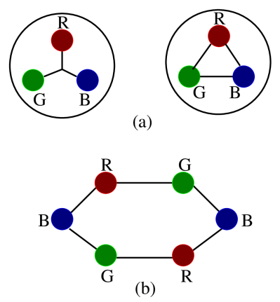
FIG. 1.: (a) Y-shaped (left) and triangular (right) arrangement of strings for a single three-quark cluster; for harmonic string the potential is identical. (b) An example of a six-quark configuration allowed in the model.

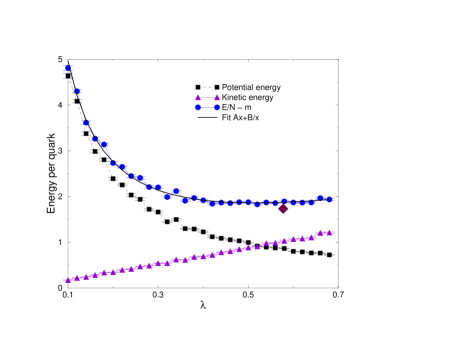
FIG. 2.: Low-density behavior of the kinetic, potential, and total energy per quark as a function of the variational parameter. The diamond indicates the energy/quark and variational parameter for an isolated nucleon. The density of the system is $\rho/\rho_{c}\!\simeq\!4\!\times\!10^{-3}$.

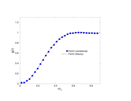
FIG. 3.: Two-body correlation function between identical quarks. The circles represent the results from the Monte-Carlo simulation while the solid line is the theoretical prediction. The density of the system is $\rho/\rho_{c}\!\simeq\!45$.

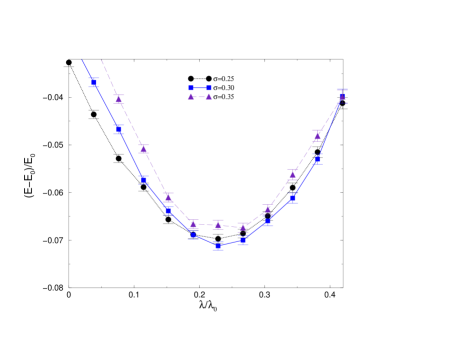
FIG. 4.: Energy-per-quark as a function of the variational parameter for three values of the strangeness-to-quark ratio. The number of quarks in the simulation is $N\!=\!120$ and the density of the system is fixed at $\rho/\rho_{c}\!=\!2.18$.

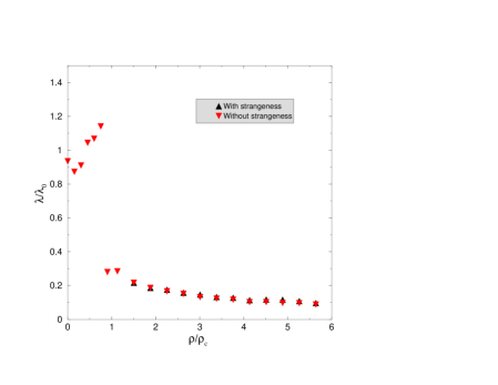
FIG. 5.: Variational parameter $\lambda$ as a function of density for systems with (up-triangles) and without (down-triangles) strangeness. The sharp drop signals the transition from three- to multi-quark configurations.

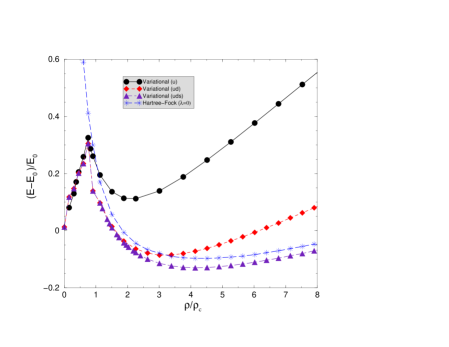
FIG. 6.: Energy per quark as a function of density for one-, two- and three-flavor systems as a function of density. The Hartree-Fock ($\lambda\!=\!0$) energy is also shown to illustrate the effect of clustering correlations. In this model three-flavor strange-quark matter is absolutely bound.

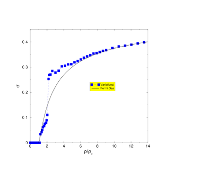
FIG. 7.: Strangeness-to-quark ratio as a function of density for the variational calculation (filled squares) and a simple Fermi-gas estimate (solid line). Note the discontinuity of the transition at $\rho/\rho_{c}\!\approx\!2.2.$

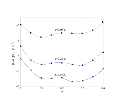
FIG. 8.: Energy-per-quark as a function of strangeness-to-quark ratio for three values of the quark density. In all three cases the variational parameter has been fixed at its optimal value. Note the competition between the two minima, particularly in the $\rho/\rho_{c}\!\approx\!2.26$ case.