Nuclear Anapole Moments

Abstract

Nuclear anapole moments are parity-odd, time-reversal-even E1 moments of the electromagnetic current operator. Although the existence of this moment was recognized theoretically soon after the discovery of parity nonconservation (PNC), its experimental isolation was achieved only recently, when a new level of precision was reached in a measurement of the hyperfine dependence of atomic PNC in ¹³³Cs. An important anapole moment bound in ²⁰⁵Tl also exists. In this paper, we present the details of the first calculation of these anapole moments in the framework commonly used in other studies of hadronic PNC, a meson exchange potential that includes long-range pion exchange and enough degrees of freedom to describe the five independent $S-P$ amplitudes induced by short-range interactions. The resulting contributions of $\pi-$, $\rho-$, and $\omega-$exchange to the single-nucleon anapole moment, to parity admixtures in the nuclear ground state, and to PNC exchange currents are evaluated, using configuration-mixed shell-model wave functions. The experimental anapole moment constraints on the PNC meson-nucleon coupling constants are derived and compared with those from other tests of the hadronic weak interaction. While the bounds obtained from the anapole moment results are consistent with the broad “reasonable ranges” defined by theory, they are not in good agreement with the constraints from the other experiments. We explore possible explanations for the discrepancy and comment on the potential importance of new experiments.

I Introduction

The strangeness-conserving ($\Delta S=0$) weak nucleon-nucleon interaction is of considerable interest. It provides the one experimentally accessible means of probing the neutral current component of the hadronic weak interaction, as this component plays no role in flavor-changing reactions. Furthermore the question of how long-range weak forces between nucleons are connected to the underlying elementary weak quark-boson couplings of the standard model is an important strong-interaction question, one with potential connections to poorly understood phenomena such as the $\Delta$ I = 1/2 rule. One of the challenges in the field has been the experimental determination of the various spin and isospin contributions to the low-energy weak $NN$ interaction, as this interaction is dwarfed by much larger strong and electromagnetic forces. The weak effects can be isolated only by precisely measuring tiny effects associated with the parity nonconservation (PNC) accompanying this interaction. Because the PNC effects are typically of relative size $\sim 10^{-7}$, only one class of elementary $NN$ scattering experiments, $\vec{p}+p$, has reached the requisite sensitivity. PNC effects have also been isolated in nuclear experiments, but only a few nuclear systems are sufficiently well understood to permit theorists to relate the observable to the underlying $NN$ interaction. For these reasons there is interest in finding new experimental constraints.

Shortly after Lee and Yang’s proposal that weak interactions violate parity, Vaks and Zeldovich [1] noted independently that an elementary particle (as well as composite systems like the nucleon or nucleus) could have a new electromagnetic moment, the “anapole moment”, corresponding to a PNC coupling to a virtual photon. One contribition to the anapole moments of hadrons would thus arise from PNC loop corrections to the electromagnetic vertex. Despite some early work on the contribution of the nucleon anapole moment to high-energy electron-nucleon scattering [2], the interest in anapole moments might have been limited to theorists had not Flambaum, Khriplovich, and collaborators [3] pointed out their enhanced effects in atomic PNC experiments in heavy atoms. As the anapole moment is spin dependent, it contributes to the small hyperfine dependence of atomic PNC. (The dominant PNC effects in such experiments arise from the coherent vector coupling of the exchanged $Z^{0}$ to the nucleus, and are thus independent of nuclear spin.) While nuclear-spin-dependent effects do arise from Vector(electron)- Axial(nucleus) $Z^{0}$ exchange, this nuclear coupling does not grow systematically with the nucleon number $A$ of the nucleus: naively, the axial coupling in an odd-$A$ nucleus is to the unpaired valence nucleon. Flambaum et al. [3] observed that the anapole moment of a heavy nucleus grows as $A^{2/3}$, so that weak radiative corrections to spin-dependent atomic PNC associated with the anapole moment would typically dominate over the corresonding tree-level $Z^{0}$ exchange for sufficiently large $A$ ($A\mathrel{\hbox to0.0pt{\lower 4.0pt\hbox{\hskip 1.0pt$\sim$}\hss}\raise 1.0pt\hbox{$>$}}$ 20). This growth means that spin-dependent atomic PNC effects should be dominated by the anapole moment – a radiative “correction” – and measurable in heavy atoms.

Nevertheless, spin-dependent atomic PNC effects are still exceedingly small, typically $\sim$ 1% of the size of nuclear-spin-independent atomic PNC effects. Despite considerable effort, only limits existed on the anapole contribution until very recently. However, with the Colorado group’s measurement [4] of atomic PNC in ¹³³Cs at the level of 0.35%, a definitive (7$\sigma$) nuclear-spin-dependent effect emerged from the hyperfine differences. This measuement is the principal motivation for the work presented here. The goal of the present study is to carry out an analysis of the ¹³³Cs anapole moment that follows as closely as possible the formalism developed and employed in other $NN$ and nuclear tests of the low-energy hadronic weak interaction [5]. That formalism is based on the finite-range PNC $NN$ potential of Desplanques, Donoghue, and Holstein (DDH), a potential that contains sufficient freedom to describe the long-range $\pi$ exchange and the short-range physics governing the five independent PNC $S-P$ $NN$ amplitudes [6]. The resulting $\pi-$, $\rho-$, and $\omega-$exchange PNC $NN$ potential is employed in estimating the loop contributions to the single-nucleon anapole moment and the exchange current and nuclear polarization contributions to the nuclear anapole moment for ¹³³Cs. We also present results for Tl, where an interesting anapole limit exists [7, 8].

The current work extends the treatment of Ref. [9] by including heavy-meson PNC contributions, thereby going beyond long-range $\pi$ exchange to the full DDH potential. This extension is crucial in describing the isospin character of both the single-nucleon and nuclear polarizability contributions to the anapole moment. The main results of our study were recently presented in a letter [10]. Here we give the technical details of the heavy-meson current and polarizability calculations, and discuss the associated shell-model calculations and their potential shortcomings. Our approach differs from most earlier calculations [3, 11, 12, 13, 14, 15] by avoiding one-body reductions of the currents and potentials: exchange currents and polarizabilities are evaluated from shell-model two-body densities matrices, modified by short-range correlation functions that mimic the effects of missing high-momentum components. We also use a form for the anapole operator in which components of the three-current constrained by current conservation are rewritten in terms of a commutator with the Hamiltonian, and thus explicitly removed.

The paper is organized as follows. In Sec. II we define the anapole moment and the electron-nucleus interaction it induces, and discuss connections with the generalized Siegert’s theorm. In Sec. III we describe the DDH PNC $NN$ interaction arising from $\pi-,\rho-$, and $\omega-$exchange and its connections with the $S-P$ amplitudes. The treatment of the one-body, exchange-current, and polarization contributions to the anapole moment are given in Sec. IV. The summation over intermediate nuclear states in the polarizability is performed by closure, after calibrating this approach in a series of more complete shell-model calculations in lighter nuclei. Other technical details – particularly the rather complicated heavy-meson exchange-current evaluations – are presented in Appendices A through D. In Sec. V experimental values for the anapole moments of ¹³³Cs and ²⁰⁵Tl are deduced from the corresponding hyperfine PNC measurements. Other tests of the low-energy PNC $NN$ interaction are discussed, and the constraints they impose on various PNC meson-nucleon couplings described. We address the issue of uncertainties in the shell-model nuclear structure calculations and attempt to assess the effects of missing correlations phenomenologically. In the concluding Sec. VI we discuss the resulting discrepancies and possible future work that would help address some of the open questions.

II The Anapole Operator and Current Conservation

In this section we describe the anapole moment in terms of a classical current distribution [16, 17]. The corresponding operator for a quantum mechanical current is obtained from a multipole expansion that satisfies the generalized Siegert’s theorem. We illustrate, in a simple one-body nuclear model, the relationship between the anapole moment and the PNC $NN$ interaction and the consequences of current conservation.

A Anapole Moments in Classical Electromagnetism

Given classical charge and current distributions, $\rho(\vec{x}^{\,\,{}^{\prime}})$ and $\vec{j}(\vec{x}^{\,\,{}^{\prime}})$, the scalar and vector potentials, $\Phi(\vec{x})$ and $\vec{A}(\vec{x})$, are obtain from integrals over the Green’s function. After a Taylor expansion around the source point $\vec{x}^{\,\,{}^{\prime}}$ one obtains

$$\Phi(\vec{x}) = \int d^{3}x^{\,\,{}^{\prime}}\frac{\rho(\vec{x}^{\,\,{}^{\prime}})}{4\pi|\vec{x}-\vec{x}^{\,\,{}^{\prime}}|}$$ (1)

$$= \int d^{3}x^{\,\,{}^{\prime}}\rho(\vec{x}^{\,\,{}^{\prime}})\{1-\vec{x}^{\,\,{}^{\prime}}\cdot\vec{\nabla}+\frac{1}{2}(\vec{x}^{\,\,{}^{\prime}}\cdot\vec{\nabla})^{2}+\cdots\}\frac{1}{4\pi|\vec{x}|},$$ (2)

$$\vec{A}(\vec{x}) = \int d^{3}x^{\,\,{}^{\prime}}\frac{\vec{j}(\vec{x}^{\,\,{}^{\prime}})}{4\pi|\vec{x}-\vec{x}^{\,\,{}^{\prime}}|}$$ (3)

$$= \int d^{3}x^{\,\,{}^{\prime}}\vec{j}(\vec{x}^{\,\,{}^{\prime}})\{1-\vec{x}^{\,\,{}^{\prime}}\cdot\vec{\nabla}+\frac{1}{2}(\vec{x}^{\,\,{}^{\prime}}\cdot\vec{\nabla})^{2}+\cdots\}\frac{1}{4\pi|\vec{x}|}.$$ (4)

In the scalar potential expansion, the first term inside the curly bracket generates the total charge (monopole) moment; the second term, the electric dipole moment; and the third term, a combination of the quadrupole and monopole charge moments[18]. For the vector potential, the first term vanishes as there is no net current. After carefully taking the constraints of current conservation and the boundedness of the current density into account (which place six constraints on the bilinear products $j(\vec{x}^{\,\,{}^{\prime}})_{i}x^{\,\,{}^{\prime}}_{j}$), there remain three independent components in the second term, corresponding to the magnetic dipole moment of a classical current distribution. Similarly, the third term involves a symmetric product of two coordinates with the current, generating 18 independent trilinear combinations, with 10 constraints. The remaining eight independent components comprise the static magnetic quadrupole moment and the $E1$ moment known as the “anapole moment” (AM).

One can extract the vector potential due to the AM explicitly,

$$\vec{A}^{(anapole)}(\vec{x})=(-\vec{a}{\nabla^{2}\over M^{2}}+{\vec{\nabla}\over M}\vec{a}\cdot{\vec{\nabla}\over M})\frac{1}{4\pi|\vec{x}|},$$ (5)

where

$$\vec{a}=\frac{M^{2}}{6}\int d^{3}x^{\,\,{}^{\prime}}\vec{x}^{\,\,{}^{\prime}}\times(\vec{x}^{\,\,{}^{\prime}}\times\vec{j}(\vec{x}^{\,\,{}^{\prime}})).$$ (6)

(We multiply and divide by $M^{2}$ for consistency with the definition of $\vec{a}$ we will later introduce via the Dirac equation.) We can remove the second term in Eq. (5) by a gauge transformation, so that

$$\vec{A}^{(anapole)}(\vec{x})={\vec{a}\over M^{2}}\delta^{(3)}(\vec{x}).$$ (7)

Current conservation allows Eq. (6) to be rewritten as

$$\vec{a}=-\frac{M^{2}}{4}\int d^{3}x^{{}^{\prime}}{x^{{}^{\prime}}}^{2}\vec{j}(\vec{x}^{{}^{\prime}}).$$ (8)

(We use the Lorentz-Heaviside unit in which $\alpha=e^{2}/4\pi\hbar c=1/137$.) Eq. (8) is often presented as the definition of the AM [3, 12, 13, 14, 15, 16, 17, 19]. However it is important to note that this form is obtained only after exploiting the constraints of current conservation.

It is apparent, for the ordinary electromagnetic current, that the associated AM operator is odd under a parity transformation. Therefore a nonzero AM requires either the introduction of an axial vector component into the current or a parity admixture in the ground state (allowing the ordinary electromagnetic current to have a nonvanishing expectation value). This requirement of PNC associates the AM with the weak interaction.

Another important property is the contact nature of the AM vector potential. Thus an atomic electron interacts with the AM of the nucleus only to the extent that its wave function penetrates the nucleus.

FIG. 1.: A toroidal current winding generates a nonzero anapole moment.

Figure 1 gives a classical picture of the anapole moment as a current winding. Although the currents on the inner and outer sides of the torus oppose one another, there is a net contribution because of the $r^{2}$ weighting (in spherical coordinates) of the current in the definition of the AM, leading to an AM that points upward. The illustrated current distribution is odd under a parity reversal, as we have noted it must be for the ordinary electromagnetic current. If, however, the current has a chirality – a small “pitch” corresponding to a left- or right-handed winding that would signal PNC – a parity-even contribution to the operator would be induced.

B The Anapole Operator

Although one could quantize Eq. (8) directly to generate the anapole moment operator, a better procedure is to avoid the assumption of current conservation, as this is often violated in nuclear models. Switching to a standard spherical multipole decomposition yields the momentum-space charge and current operators [20]

$$\rho(\vec{q}) = \sum_{J,M}(-i)^{J}4\pi Y_{JM}^{*}(\Omega_{q})M_{JM}^{coul}(q);$$ (9)

$$\vec{j}_{\lambda}(\vec{q}) = \sum_{J,M}(-i)^{J}\sqrt{2\pi(2J+1)}{\mathcal{D}}_{M\lambda}^{(J)}(-\phi_{q},-\theta_{q},\phi_{q})[T_{JM}^{el}(q)-\lambda T_{JM}^{mag}(q)],$$ (10)

and the associated charge, transverse electric, and transverse magnetic multipole projections of definite angular momentum and (in the absence of PNC) parity

$$M_{JM}^{coul}(q) = \int d^{3}x\,\,j_{J}(qx)Y_{JM}(\Omega_{x})\rho(\vec{x});$$ (11)

$$T_{JM}^{el}(q) = \int d^{3}x\,\,\frac{1}{q}\vec{\nabla}\times[j_{J}(qx)\vec{Y}^{M}_{JJ1}(\Omega_{x})]\cdot\vec{j}(\vec{x});$$ (12)

$$T_{JM}^{mag}(q) = \int d^{3}x\,\,j_{J}(qx)\vec{Y}^{M}_{JJ1}(\Omega_{x})\cdot\vec{j}(\vec{x}),$$ (13)

where $\vec{q}$ is the (outgoing) three-momentum transfer, $j_{J}$ the spherical Bessel function, $Y_{JM}$ and $\vec{Y}^{M}_{JJ1}$ the ordinary and vector spherical harmonics, and ${\mathcal{D}}_{M\lambda}^{(J)}(-\phi_{q},-\theta_{q},\phi_{q})$ the rotation matrix.

The transformation properties of the possible multipole moments under parity (P) and time-reversal (T) are listed in Table I. Systems that are parity and time-reversal invariant can have only even-rank Coulomb moments (charge, charge quadrupole, etc.) and odd-rank transverse magnetic moments (magnetic dipole, magnetic octupole, etc.). The P- and T-odd moments, which would arise in the standard model from small CP-violating contributions to the weak interaction, correspond to the odd-rank Coulomb and even-rank transverse magnetic multipoles (electric dipole, magnetic quadrupole, etc.). The PNC but T-even moments, which would arise from the usual weak interaction, correspond to the odd-rank transverse electric multipoles, with the lowest of these being the dipole moment known as the anapole moment.

TABLE I.: Properties of multipole moments under parity and time reversal. A slash (no slash) denotes odd (even) behavior.

	$M^{coul}$	$T^{el}$	$T^{mag}$
$J=0$	$PT$
$J=1$	$P\!\!\!\!/T\!\!\!\!/$	$P\!\!\!\!/T$	$PT$
$J=2$	$PT$	$PT\!\!\!\!/$	$P\!\!\!\!/T\!\!\!\!/$
$J=3$	$P\!\!\!\!/T\!\!\!\!/$	$P\!\!\!\!/T$	$PT$
$\vdots$	$\vdots$	$\vdots$	$\vdots$

For consistency with Eq. (7), we require

$$\nabla^{2}\vec{A}(\vec{x})=-\vec{j}(\vec{x}),$$ (14)

which then defines the anapole operator

$$a_{1\lambda}=\lim_{\vec{q}^{2}\rightarrow 0}\frac{-i\sqrt{6\pi}M^{2}}{{}_{\vec{q}^{2}}}T_{1\lambda}^{el}.$$ (15)

The simplest case is the general expression for the matrix element of a conserved four-current for a free spin-${1\over 2}$ particle

$$\bar{U}(p^{\prime})J^{\mu}(q)U(p) = \bar{U}(p^{\prime})(F_{1}(q^{2})\gamma^{\mu}-i{F_{2}(q^{2})\over 2M}\sigma^{\mu\nu}q_{\nu}$$ (17)

$$+{a(q^{2})\over M^{2}}(\not qq^{\mu}-q^{2}\gamma^{\mu})\gamma_{5}-i{d(q^{2})\over M}\sigma^{\mu\nu}q_{\nu}\gamma_{5})U(p).$$

from which the four moments of Table I can be immediately identified. The two vector terms define the charge $F_{1}(q^{2})$ and magnetic $F_{2}(q^{2})$ form factors. The axial terms that follow are the anapole and electric dipole terms, respectively. The anapole term reduces in the nonrelativistic limit to

$${a(q^{2})\over M^{2}}(\not qq^{\mu}-q^{2}\gamma^{\mu})\gamma_{5} \rightarrow {a(q^{2})\over M^{2}}\vec{q}^{~{}2}(\vec{\sigma}-\hat{q}\hat{q}\cdot\vec{\sigma})$$ (18)

$$= {a(q^{2})\over M^{2}}\vec{q}^{~{}2}\vec{\sigma}_{\perp},$$ (19)

showing that the current is transverse and spin-dependent. From this current we then have the AM operator for a nonrelativistic point particle

$$\hat{a}_{1\lambda}=a(0)\sigma_{1\lambda}.$$ (20)

C Current Conservation and the Extended Siegert’s Theorem

The anapole operator $a_{1\lambda}$ has been defined in terms of $T^{el}_{1\lambda}$, and it is well known that this operator can be transformed into other forms by exploiting the continuity equation. These forms are equivalent in calculations where consistent charge and current operators can be constructed and exact matrix elements evaluated. However we are interested in nuclear calculations where, when one goes beyond the simplest descriptions to models that treat the interactions among the nucleons, current conservation is not preserved. We lack a prescription for constructing the many-body currents consistently that are necessary for current conservation, and for addressing the renormalizations that account for the limited Hilbert spaces employed in nuclear models. In such cases there is a preferred form for $T^{el}_{1\lambda}$, the form in which all components of the three-current constrained by current conservation are reexpressed in terms of the charge operator.

A familiar example is the case of $E1$ transitions generated by the ordinary electromagnetic current. Then $T^{el}_{1\lambda}$ generates a one-body operator proportional to $\vec{p}/M$, which is of order $v/c$, where $v$ is the nucleon velocity. It can be shown that the exchange current contribution to $T^{el}_{1\lambda}$ is also of this order. As the exchange currents, in general, cannot be constructed faithfully, it follows that errors will arise that are necessarily of leading order in the velocity.

Siegert [21] showed that the situation could be greatly improved by exploiting the continuity equation

$$\vec{\nabla}\cdot\vec{j}(\vec{x})=-i[H,\rho(\vec{x})]$$ (21)

to write $T^{el}_{J}$, in the long-wavelength limit, entirely in terms of the charge operator. This generates the familiar dipole form of the transverse electric operator, proportional to $\omega\vec{r}$, where $\omega$ is the energy transfer. The importance of this rewriting is that the charge operator, which is of order $(v/c)^{0}$, has exchange current corrections only of order $(v/c)^{2}$, or of relative size $\sim$ 1%. Thus the Siegert’s form of the $E1$ operator is a far more controlled operator in nuclear calculations.

A form of $T^{el}_{1\lambda}$ consistent with Siegert’s theorem is in common use [22]

$$T_{JM}^{el^{\prime}}(q) \doteq \frac{E_{i}-E_{f}}{q}(\frac{J+1}{J})^{1/2}M_{JM}^{coul}(q)$$ (23)

$$-i(\frac{2J+1}{J})^{1/2}\int d^{3}x\,\,j_{J+1}(qx)\vec{Y}^{M}_{JJ+11}(\Omega_{x})\cdot\vec{j}(\vec{x}),$$

where $\doteq$ means the equality holds after taking matrix elements $\langle f|\hat{O}|i\rangle$. This form has the correct leading-order behavior for transitions due to the first term, with the second term vanishing as $q\rightarrow 0$. But for a static moment, the first term vanishes; the leading-order behavior is then governed by the second term, which the naive Siegert’s theorem does not properly constrain.

However the extension of Siegert’s theorem to arbitrary $q$ was derived by Friar and Fallieros [23, 22]: at every order in $q$ those components of the current constrained by current conservation are identified and rewritten in terms of the charge operator. The result is

$$T_{JM}^{el^{\prime\prime}}(q) \doteq \frac{E_{i}-E_{f}}{q}(\frac{J+1}{J})^{1/2}\int d^{3}x\,\,\frac{(qx)^{J}}{(2J+1)!!}g_{J}(qx)Y_{JM}(\Omega_{x})\rho(\vec{x})$$ (25)

$$-\frac{q}{J+2}\int d^{3}x\,\,\frac{(qx)^{J}}{(2J+1)!!}h_{J}(qx)\vec{Y}^{M}_{JJ+11}(\Omega_{x})\cdot(\vec{x}\times\vec{j}(\vec{x})),$$

where $g_{J}$ and $h_{J}$ are polynomials in $q$ [23]. Combining Eq. (25) and Eq. (15) one finds [9]

$$a_{\lambda}=-\frac{M^{2}}{9}\int d^{3}x\,\,x^{2}[j_{\lambda}(\vec{x})+\sqrt{2\pi}(Y_{2}(\Omega x)\otimes\vec{j}(\vec{x}))_{\lambda}]$$ (26)

This is the AM operator form used here and in our earlier work; to our knowledge all other analyses have been based on the naive form of Eq. (8).

We stress that the three transverse electric operators $T^{el}$ ,$T^{el^{\prime}}$, and $T^{el^{\prime\prime}}$ are equivalent for simple one-body models which ignore nucleon-nucleon interactions, provided the resulting one-body currents are properly generated by minimal substitution. The differences in these operators arise when they are used in more realistic calculations.

D Simple Examples

In this section we illustrate how this equivalence is manifested in non-interacting shell model calculations of the nuclear AM of ¹³³Cs. The PNC interaction is also taken to be a one-body effective potential, $H^{(1)}_{PNC}$.

The elements of the calculation include:

1. Extreme single-particle forms for the ground-state nuclear wave function. As ¹³³Cs is an odd-even nucleus with $J$ = 7/2⁺, the odd proton is placed in the $1g_{7/2}$ shell, outside an otherwise fully spin-paired closed core.

2. The strong Hamiltonian is a one-body harmonic oscillator potential with spin-orbit interaction. While this description is primitive, it does yield the proper ground-state spin and parity for the (nearly spherical) nucleus ¹³³Cs. The harmonic oscillator wave functions allow analytic calculations of polarizabilities, etc.

3. $H^{(1)}_{PNC}$ is treated perturbatively: only linear terms are retained.

Thus the resulting Hamiltonian is

$$H=H_{0}+H^{(1)}_{PNC}\,,$$ (27)

with

$$H_{0} = \sum^{A}_{i=1}\frac{\vec{p}(i)^{2}}{2M}+\frac{1}{2}M\omega^{2}\vec{x}(i)^{2}-f\vec{s}(i)\cdot\vec{l}(i);$$ (28)

$$H^{(1)}_{PNC} = \sum^{A}_{i=1}\frac{g_{S}+g_{V}\tau_{3}(i)}{2M}\vec{\sigma}(i)\cdot\vec{p}(i),$$ (29)

where $\omega$ is related to the harmonic oscillator size parameter $b$ by $\omega=1/Mb^{2}$, the spin-orbit strength $f$ can be determined from shell splittings near the $3s2d1g$ shell, and $g_{S}$ and $g_{V}$, the isoscalar and isovector strengths in the one-body PNC potential, can be chosen to represent the average potential exerted by the core nucleons. The analytic expressions we obtain illustrate the functional dependence on all of these parameters. Thus we are not concerned here with specific numerical values.

By minimal substitution

$$H\rightarrow H+e\Phi\quad;\quad\vec{p}\rightarrow\vec{p}-e\vec{A},$$ (30)

one can derive the charge and current densities to order $1/M$,

$$\rho(\vec{x})=e\sum^{A}_{i=1}\frac{1+\tau_{3}(i)}{2}\delta^{(3)}(\vec{x}-\vec{x}_{i}),$$ (31)

and

$$\vec{j}_{conv}(\vec{x}) = e\sum^{A}_{i=1}\frac{1+\tau_{3}(i)}{2M}\{\vec{p}(i),\delta^{(3)}(\vec{x}-\vec{x}_{i})\}_{sym}\,;$$ (33)

$$\vec{j}_{mag}(\vec{x}) = e\sum^{A}_{i=1}\frac{\mu_{S}+\mu_{V}\tau_{3}(i)}{2M}\vec{\nabla}\times(\vec{\sigma}(i)\delta^{(3)}(\vec{x}-\vec{x}_{i}));$$ (34)

$$\vec{j}_{s.o.}(\vec{x}) = e\sum^{A}_{i=1}\frac{1+\tau_{3}(i)}{2}\frac{f}{2}\vec{x}(i)\times\vec{\sigma}(i)\delta^{(3)}(\vec{x}-\vec{x}_{i});$$ (35)

$$\vec{j}_{PNC}(\vec{x}) = e\sum^{A}_{i=1}\frac{1+\tau_{3}(i)}{2M}\frac{g_{S}+g_{V}}{2}\vec{\sigma}(i)\delta^{(3)}(\vec{x}-\vec{x}_{i}),$$ (36)

where the subscripts $conv,mag,s.o.$, and $PNC$ denote the current densities arising from convection (kinetic energy), magnetization (intrinsic nucleon spin), the spin-orbit interaction, and the PNC potential, respectively. The first three are vector currents while the last is axial vector. Current conservation is then easily verified

$$\vec{\nabla}\cdot(\vec{j}_{conv}(\vec{x})+\vec{j}_{mag}(\vec{x})+\vec{j}_{s.o.}(\vec{x})+\vec{j}_{PNC}(\vec{x}))=-i[H_{0}+H^{(1)}_{PNC}\,,\,\rho(\vec{x})].$$ (37)

Contributions to the AM are generated by the axial-vector current acting between the unperturbed nuclear ground state and by vector currents that contribute because $H^{(1)}_{PNC}$ perturbs the ground state,

$$\langle\psi|T^{el}_{1}|\psi\rangle = \langle\psi_{0}|T^{el(A)}_{1}|\psi_{0}\rangle$$ (39)

$$+\sum_{\chi_{0}}(\frac{\langle\psi_{0}|T^{el(V)}_{1}|\chi_{0}\rangle\langle\chi_{0}|H^{(1)}_{PNC}|\psi_{0}\rangle}{E_{\psi_{0}}-E_{\chi_{0}}}+H.c.),$$

where $\psi_{0}$ and $\chi_{0}$s are single particle unperturbed eigenfunctions of definite (and opposite) parities, and the superscripts (A) and (V) label the components of $T^{el}_{1}$ generated by the axial-vector and vector currents, respectively.

The special case of no spin-orbit interaction is interesting because the first-order perturbed wave function (in fact, the result can be generalized to all orders) is given by the Michel transformation [24]

$$\psi_{0}(\vec{x})\rightarrow\psi(\vec{x}) = (1-ig\frac{\vec{\sigma}}{2}\cdot\vec{x})\psi_{0}(\vec{x})$$ (40)

$$\cong e^{-i\vec{s}\cdot(gx)\hat{x}}\psi_{0}(\vec{x}),$$ (41)

where $g=g_{S}\pm g_{V}$ for a proton(+) or neutron(-). Eq. (41) shows that $H^{(1)}_{PNC}$ generates a spin rotation along the radial direction characterized by a small angle proportional to $g$ and to the distance to the center of the nucleus. Consider an $S_{1/2}$ state aligned along the $+z$ axis. The spin probability around a ring, centered at the origin, would be uniform and in the $+z$ direction: we visualize this as a uniform array of up-spinors. When the weak interaction is turned on, the Michel rotation will produce a spin helix [16] structure for this chain of spinors as shown in Fig. 2. If we picture each spin as a small current loop, the combination of all horizontal spin components $S_{//}$ can be viewed as a toroidal current winding producing an AM, as discussed in Sec. II A.

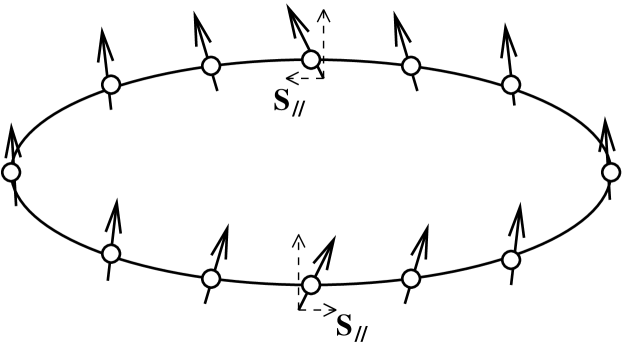
FIG. 2.: Spin helix structure due to the parity mixing.

Moreover, if the Michel transformed wave function is used in a calculation of the AM, one finds that the contributions from $\vec{j}_{PNC}$ and $\vec{j}_{conv}$ cancel exactly, so that $\vec{j}_{mag}$ is entirely responsible for the AM. Even with the inclusion of the spin-orbit interaction, the magnetization current remains the major contribution to the AM [3].

The sum over intermediate states in Eq. (39) simplies considerably in the harmonic oscillator since the momentum operator $\vec{p}$ only generates transitions of one $\hbar\omega$. Thus the transitions that must be consider in the extreme single-particle limit are the simple $1p$ and $2p1h$ single-shell transitions of Fig. 3 [15].

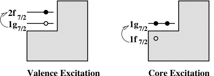
FIG. 3.: Valence and core excitations produced by the PNC potential acting on an extreme single-particle harmonic oscillation ground state. The levels illustrated are appropriate for ¹³³Cs.

Some preliminary algebraic manipulations are helpful. Using the commutation relation

$$[\frac{\vec{p}^{2}}{2M}+\frac{1}{2}M\omega^{2}\vec{x}^{2},\vec{x}]=-i\frac{\vec{p}}{M},$$ (42)

the PNC one-body potential can be rewritten as

$$H^{(1)}_{PNC} = \frac{g}{2M}\vec{\sigma}\cdot\vec{p}$$ (43)

$$= i\frac{g}{2M}([H_{0},\vec{\sigma}\cdot\vec{x}]+\frac{f}{2}[\vec{\sigma}\cdot\vec{l},\vec{\sigma}\cdot\vec{x}]).$$ (44)

Using this result in the polarization sum yields

$$a^{(pol)} = i\frac{gM^{2}}{2}\langle i|[\vec{\sigma}\cdot\vec{x},T_{1}^{el(V)}]|i\rangle$$ (46)

$$+\frac{gM^{2}}{2}f\sum_{n}\langle i|\vec{\sigma}\cdot(\vec{x}\times\vec{l})|n\rangle\langle n|T^{el(V)}_{1}|i\rangle/(E_{i}-E_{n})+H.c.$$

As a typical value for the nuclear spin-orbit strength is $f/\omega\equiv\alpha\sim 0.1$, one can work to first order in $f$, yielding for the various AM contributions

$$a^{(conv)} \cong \frac{gM}{8}\langle i|x^{2}\vec{\sigma}|i\rangle$$ (48)

$$-\frac{gM}{4}f\sum_{n}\langle i|\vec{\sigma}\cdot(\vec{x}\times\vec{l})|n\rangle\langle n|\frac{1}{2}(x^{2}\vec{p}-i\vec{x})|i\rangle/(E_{i}-E_{n})+H.c.\,,$$

$$a^{(mag)} \cong \frac{gM}{4}\mu\Big{\{}\langle i|(\vec{\sigma}\cdot\vec{x})\vec{x}-x^{2}\vec{\sigma}|i\rangle$$ (50)

$$-f\sum_{n}\langle i|\vec{\sigma}\cdot(\vec{x}\times\vec{l})|n\rangle\langle n|\frac{1}{2}\vec{\sigma}\times\vec{x}|i\rangle/(E_{i}-E_{n})+H.c.\Big{\}}\,,$$

$$a^{(s.o.)} \cong -\frac{gM^{2}}{8}f\langle i|x^{2}((\vec{\sigma}\cdot\vec{x})\vec{x}-x^{2}\vec{\sigma})|i\rangle\,,$$ (51)

$$a^{(PNC)} \cong -\frac{gM}{8}\langle i|x^{2}\vec{\sigma}|i\rangle\,.$$ (52)

As the $O(f^{0})$ terms from $a^{(conv)}$ and $a^{(PNC)}$ exactly cancel, $a^{(mag)}$ determines the leading-order (LO) contribution

$$a_{LO}=\frac{gM}{4}\mu\langle i|(\vec{\sigma}\cdot\vec{x})\vec{x}-x^{2}\vec{\sigma}|i\rangle.$$ (53)

For the next-to-leading-order (NLO) $O(f^{1})$ contributions, we approximate $E_{i}-E_{n}\simeq-\hbar\omega$ (as the spin-orbit correction to this are higher order) and invoke closure

$$a^{(conv)}_{NLO} \simeq \frac{gM}{4}\alpha\langle i|\{\vec{\sigma}\cdot(\vec{x}\times\vec{l}),\frac{1}{2}(x^{2}\vec{p}-\vec{x})\}|i\rangle,$$ (54)

$$a^{(mag)}_{NLO} \simeq \frac{gM}{4}\alpha\mu\langle i|\{\vec{\sigma}\cdot(\vec{x}\times\vec{l}),\frac{1}{2}(\vec{\sigma}\times\vec{x})\}|i\rangle.$$ (55)

Therefore, assuming these matrix elements are of the same order of magnitude, one obtains for the relative sizes

$$|a^{(conv)}_{NLO}/a_{LO}| \sim \left|\frac{\alpha}{\mu}\right|,$$ (56)

$$|a^{(mag)}_{NLO}/a_{LO}| \sim \left|\alpha\right|,$$ (57)

$$|a^{(s.o.)}/a_{LO}| \sim \left|\frac{\alpha}{2\mu}\right|\frac{\langle x^{2}\rangle}{b^{2}}\sim A^{1/3}\left|\frac{\alpha}{2\mu}\right|\sim\left|\alpha\right|,$$ (58)

where in the last line we assume an odd-proton nucleus with $A\sim 100$, similar to Cs.

In Table II we present our results for the AM of ¹³³Cs in this single-particle scheme using the four different $T_{1}^{el}$s discussed previously ($T_{1}^{el}$,$T_{1}^{el\,\,^{\prime}}$,$T_{1}^{el\,\,^{\prime\prime}}$, and the one from the Cartesian decomposition using Eq. (15) and Eq. (8)) to define our anapole operator. Agreement is achieved only when: i) all the currents–$conv,mag,s.o.$, and $PNC$–and ii) a complete set of excitations–valence and core–are considered. This illustrates a point made earlier, that the use of incomplete current operators or Hilbert spaces breaking current conservation will in general lead to difficulties.

TABLE II.: Matrix elements corresponding to four choices of the anapole operator. Note the dimensionless parameter $\alpha\equiv f/\omega=fMb^{2}$, where $b$ is the oscillator parameter. The results are in units of $C\equiv 4\pi\sqrt{\frac{2}{7}}(g_{S}+g_{V})Mb^{2}$, another dimensionless quantity.

$\langle||a||\rangle/e$	$T_{1}^{el}$	$T_{1}^{el^{\prime}}$	$T_{1}^{el^{\prime\prime}}$	$Cartesian$
$conv$	$\frac{-1.1}{1-4\alpha}+\frac{-5.4}{1+4\alpha}$	$\frac{-2.8}{1-4\alpha}+\frac{-2.7}{1+4\alpha}$	$\frac{-4/3}{1-4\alpha}+\frac{-6}{1+4\alpha}$	$\frac{0.5}{1-4\alpha}+\frac{-10.125}{1+4\alpha}$
$mag$	$\frac{11.16}{1-4\alpha}+\frac{50.22}{1+4\alpha}$	$\frac{11.16}{1-4\alpha}+\frac{50.22}{1+4\alpha}$	$\frac{11.16}{1-4\alpha}+\frac{50.22}{1+4\alpha}$	$\frac{11.16}{1-4\alpha}+\frac{50.22}{1+4\alpha}$
$s.o.$	$\frac{-15.6\alpha}{1-4\alpha}+\frac{-30.6\alpha}{1+4\alpha}$	$\frac{-8.8\alpha}{1-4\alpha}+\frac{-19.9\alpha}{1+4\alpha}$	$\frac{-44\alpha/3}{1-4\alpha}+\frac{-33\alpha}{1+4\alpha}$	$\frac{-22\alpha}{1-4\alpha}+\frac{-49.5\alpha}{1+4\alpha}$
$PNC$	$13/2$	$11/2$	$22/3$	$77/8$
$Tot.$	$\frac{11.16-20\alpha}{1-4\alpha}+\frac{50.22-9\alpha}{1+4\alpha}$	same	same	same

The table also shows that the contribution of the magnetization current, which is separately conserved ($\vec{\nabla}\cdot\vec{j}^{(mag)}=0)$, is independent of the choice of the anapole operator. This term is entirely responsible for the leading $O(\alpha^{0})$ result (given the $conv$–$PNC$ cancellation in this order). It is also apparent that the NLO contribution attributed to a given current depends on the anapole operator chosen: it is the sum over all contributions, not individual contributions, that is kept constant in calculations satisfying current conservation. The numerical value of the LO contribution (61.4) is reduced by $\sim$ 20% to 50.5 when the NLO contributions are included ($\alpha$ = 0.1), consistent with our earlier assertion that these corrections are perturbations.

III The PNC Nucleon-Nucleon Potential

The AM calculations presented here are the first to employ an $NN$ weak potential sufficiently general to describe long-range $\pi$ exchange and all five short-range $S-P$ $NN$ amplitudes. This section summarizes the isospin structure of the $\Delta S$ = 0 hadronic weak interaction and its description in terms of $\pi-$, $\rho-$, and $\omega-$exchange.

A The Isospin Structure of the Hadronic Weak Interaction

The standard model specifies the weak charged and neutral currents, $J_{W}$ and $J_{Z}$, associated with the absorption/emission of weak bosons by quarks [25]. The couplings to the light quarks (u,d,s) are

$$J^{\mu}_{W} = \cos\theta_{C}\bar{u}\gamma^{\mu}(1-\gamma_{5})d+\sin\theta_{C}\bar{u}\gamma^{\mu}(1-\gamma_{5})s\,;$$ (59)

$$J^{\mu}_{Z} = \frac{1}{\sqrt{2}\cos\theta_{W}}\{\bar{u}\gamma^{\mu}(1-\frac{8}{3}\sin^{2}\theta_{W}+\gamma_{5})u-\bar{d}\gamma^{\mu}(1-\frac{4}{3}\sin^{2}\theta_{W}+\gamma_{5})d$$ (61)

$$-\bar{s}\gamma^{\mu}(1-\frac{4}{3}\sin^{2}\theta_{W}+\gamma_{5})s\},$$

where $\theta_{C}$ is the Cabbibo angle, with $\sin\theta_{C}\sim.22$ and $\theta_{W}$ is the Weinberg angle, with $\sin^{2}\theta_{W}\sim 0.23$. The effective quark-quark weak interaction at low energies can be described by a phenomenological current-current Lagrangian

$${\mathcal{L}}_{Weak}=\frac{G_{F}}{\sqrt{2}}(J^{{\dagger}}_{W}J_{W}+J_{W}J_{W}^{{\dagger}}+J^{{\dagger}}_{Z}J_{Z}),$$ (62)

By assigning proper isospin and strangeness quantum number to each quark field, we can decompose these hadronic currents

$$J_{W} = \cos\theta_{C}J^{(1,0)}_{W}+\sin\theta_{C}J^{(\frac{1}{2},1)}_{W};$$ (63)

$$J_{Z} = J^{(1,0)}_{Z}+J^{(0,0)}_{Z},$$ (64)

where the first superscript denotes the change in isospin ($\Delta I$), and the second in strangeness ($\Delta S$). The current $J^{(1,0)}_{W}$ drives the $u\rightarrow d$ transition, while $J^{(\frac{1}{2},1)}_{W}$ drives the $u\rightarrow s$ transition. We can construct the strangeness conserving ($\Delta S$=0) hadronic weak interaction Lagrangian density

$${\mathcal{L}}^{(\Delta S=0)}_{Weak} = \frac{G_{F}}{\sqrt{2}}\bigg{(}(\cos^{2}\theta_{C}J^{(1,0){\dagger}}_{W}J^{(1,0)}_{W}+\sin^{2}\theta_{C}J^{(\frac{1}{2},1){\dagger}}_{W}J^{(\frac{1}{2},1)}_{W}+H.c.)$$ (65)

$$+ J^{(1,0){\dagger}}_{Z}J^{(1,0)}_{Z}+J^{(1,0){\dagger}}_{Z}J^{(0,0)}_{Z}+J^{(0,0){\dagger}}_{Z}J^{(1,0)}_{Z}+J^{(0,0){\dagger}}_{Z}J^{(0,0)}_{Z}\bigg{)}.$$ (66)

An important aspect of this Lagrangian density is its isospin content. The symmetric product of two $J^{(1,0)}_{W}$ currents forms $\Delta I=0$ (isoscalar) and $\Delta I=2$ (isotensor) interactions, while the symmetric product of two $J^{(\frac{1}{2},0)}_{W}$ currents forms a $\Delta I=1$ (isovector) interaction. Therefore the charged current weak $NN$ interaction in the $\Delta I=1$ channel is suppressed by $\tan^{2}\theta_{C}$ relative to the $\Delta I=0$ or $2$ contributions. As there is no isovector suppression for the neutral current, one concludes that the $\Delta I=1$ $NN$ channel provides experimentalists their best opportunity for studying the neutral current component of the hadronic weak interaction.

The physical states are strongly interacting composites, nucleons and mesons. The strong interaction dresses the underlying quark-boson couplings, and we have not yet developed the theoretical tools needed to evaluate the strong effects quantitatively. The physical couplings associated with the effective operators for nucleons and mesons are thus expected to differ – perhaps substantially – from the underlying bare couplings. One famous example of this is the $\Delta I=1/2$ rule in strangeness-changing weak decays: in experiments one finds a strong enhancement of $\Delta I=1/2$ over $\Delta I=3/2$ amplitudes, relative to expectations based on the underlying standard-model couplings and efforts to evaluate strong renormalizations. One reason for the interest in PNC is the hope that we can learn more about such strong effects by adding precise data on $\Delta S=0$ weak hadronic interactions.

B Meson Exchange and the Long-range PNC $NN$ Potential

The most straightforward contribution to the PNC nuclear potential is from the direct exchange of $W^{\pm}$and $Z^{0}$ between nucleons. Because of the small Compton wavelengths of these bosons ($\sim$ 0.002 fm) direct exchanges effectively occur only when two nucleons overlap. We do not yet have an adequate understanding of such short-range contributions to either the PNC or parity-conserving (PC) $NN$ interactions. Fortunately, for energies characteristic of bound nucleons, the $NN$ interaction takes place primarily at distances large compared to the nucleon size. This is due in part to the strong repulsion in the $NN$ interaction at short distances, and in part because nuclei are moderately dilute Fermi systems. Thus we expect long-range contributions, which can be described without explicit reference to the structure of the nucleon, to dominate the PNC interaction at low energies.

The strong PC $NN$ interaction at low energies ($\mathrel{\hbox to0.0pt{\lower 4.0pt\hbox{\hskip 1.0pt$\sim$}\hss}\raise 1.0pt\hbox{$<$}}$ 400 MeV) has been quite successfully modeled in terms of meson-exchange potentials. The complicated short-distance quark and gluon dynamics governing this interaction are parameterized by various meson-nucleon couplings and phenomenological form factors constrained by experiment. This meson-exchange strong interaction model can be enlarged to include the weak PNC $NN$ interaction by replacing one of the strong meson-nucleon couplings by a weak coupling. All of the physics of $W$ and $Z$ exchange between quarks – and the attendant strong interaction dressing – is buried inside the weak meson-nucleon vertices. As in the case of the strong $NN$ interaction, the weak vertices depend on momentum-independent meson-nucleon couplings and phenomenological form factors. For this model to make sense, one should, at a minimum, be able to derive a consistent and reliable set of meson-nucleon couplings from PNC observables. Should such a set emerge, the longer term goal would be to develop a first-principles understanding of the relationship between the effective hadronic couplings and the underlying standard model bare couplings, dressed by a complicated soup of strong quark-quark interactions.

In developing a sensible meson-exchange model for the PNC $NN$ force, one must first truncate the tower of possible dynamical mesons, effectively “integrating out” those which do not contribute explicitly to the interaction. At small center-of-mass energies light mesons dominate the PNC potential because they have longer ranges. Candidates below the chiral symmetry breaking scale of $\sim$ 1 GeV include the pseudoscalar mesons $\pi$(140MeV), $\eta$(549MeV), and $\eta^{{}^{\prime}}$(958MeV); the scalar mesons S(975 MeV) and $\delta$(983MeV); and the vector mesons $\rho$(769MeV), $\omega$(783MeV) and $\phi$(1020MeV). One could also consider crossed two-pion exchanges, etc. Barton’s theorem [26], which states that CP invariance forbids any coupling between neutral $J$=0 mesons and on-shell nucleons, helps to restrict the possibilities, eliminating exchanges of $\pi^{0}$, $\eta$, $\eta^{{}^{\prime}}$, $S$, and $\delta^{0}$ (to the extent that CP violation can be ignored). Furthermore McKellar and Pick have argued that $\delta^{\pm}$ exchange can be regarded as a form factor correction to $\pi^{\pm}$ exchange [27], and $\phi$ is strongly suppressed relative to $\rho$ and $\omega$. This motivates a PNC potential based on $\pi^{\pm}$, $\rho^{0}$, $\rho^{\pm}$, and $\omega^{0}$ exchanges. (We will present below another argument that will make this potential seem less arbitrary.)

The PC and PNC meson-nucleon interaction Lagrangian density in the $\pi-$, $\rho-$, and $\omega-$exchange model is

$${\mathcal{L}}_{PC} = ig_{\pi NN}\overline{N}^{\,\,{}^{\prime}}\gamma_{5}\vec{\tau}\cdot\vec{\pi}N-g_{\rho NN}\overline{N}^{\,\,{}^{\prime}}(\gamma_{\mu}-i\frac{\mu_{V}}{2M}\sigma_{\mu\nu}q^{\nu})\vec{\tau}\cdot\vec{\rho}^{\mu}N$$ (68)

$$-g_{\omega NN}\overline{N}^{\,\,{}^{\prime}}(\gamma_{\mu}-i\frac{\mu_{S}}{2M}\sigma_{\mu\nu}q^{\nu})\omega^{\mu}N,$$

$${\mathcal{L}}_{PNC} = -\frac{f_{\pi}}{\sqrt{2}}\overline{N}^{\,\,{}^{\prime}}(\vec{\tau}\times\vec{\pi})_{3}N+\overline{N}^{\,\,{}^{\prime}}\Big{(}h^{0}_{\rho}\vec{\tau}\cdot\vec{\rho}^{\mu}+h_{\rho}^{1}\rho^{\mu}_{3}+\frac{h_{\rho}^{2}}{2\sqrt{6}}(3\tau_{3}\rho^{\mu}_{3}-\vec{\tau}\cdot\vec{\rho}^{\mu})\Big{)}\gamma_{\mu}\gamma_{5}N$$ (70)

$$+\overline{N}^{\,\,{}^{\prime}}(h^{0}_{\omega}\omega^{\mu}+h^{1}_{\omega}\tau_{3}\omega^{\mu})\gamma_{\mu}\gamma_{5}N,$$

where $g_{\pi NN}$, $g_{\rho NN}$, and $g_{\omega NN}$ are the strong $\pi-$, $\rho-$, and $\omega-$nucleon coupling constants and $f_{\pi}$, $h^{(0,1,2)}_{\rho}$, and $h^{(0,1)}_{\omega}$ (the superscripts denote the rank of isospin) are the weak $\pi-$, $\rho-$, and $\omega-$nucleon coupling constants. (In the literature $f_{\pi}$ is also frequently called $h_{\pi}$ or $h_{\pi}^{1}$.) Note that the $\gamma_{5}$ convention is that of Bjorken and Drell, and that $q$ is the outgoing momentum of the produced meson. (Both of these conventions are opposite in sign to those of [6].) Evaluating the one-boson exchange diagrams, where one of the vertices is PC and the other PNC, and making a non-relativistic reduction, one obtains the PNC $NN$ potential

$$H^{(2)}_{PNC}(\vec{r}) = \frac{iF_{\pi}}{M}[\vec{\tau}(1)\times\vec{\tau}(2)]_{3}[\vec{\sigma}(1)+\vec{\sigma}(2)]\cdot\vec{u}_{\pi}(\vec{r})$$ (75)

$$+\frac{1}{M}\Bigg{(}\bigg{\{}F_{0}\vec{\tau}(1)\cdot\vec{\tau}(2)+\frac{F_{1}}{2}[\tau(1)_{3}+\tau(2)_{3}]+\frac{F_{2}}{2\sqrt{6}}[3\tau_{3}(1)\tau_{3}(2)-\vec{\tau}(1)\cdot\vec{\tau}(2)]\bigg{\}}$$

$$\times\{(1+\mu_{V})i[\vec{\sigma}(1)\times\vec{\sigma}(2)]\cdot\vec{u}_{\rho}(\vec{r})+[\vec{\sigma}(1)-\vec{\sigma}(2)]\cdot\vec{v}_{\rho}(\vec{r})\}$$

$$+\bigg{\{}G_{0}+\frac{G_{1}}{2}[\tau_{3}(1)+\tau_{3}(2)]\bigg{\}}\times\{(1+\mu_{S})i[\vec{\sigma}(1)\times\vec{\sigma}(2)]\cdot\vec{u}_{\omega}(\vec{r})$$

$$+[\vec{\sigma}(1)-\vec{\sigma}(2)]\cdot\vec{v}_{\omega}(\vec{r})\}+\frac{1}{2}[\tau_{3}(1)-\tau_{3}(2)][\vec{\sigma}(1)+\vec{\sigma}(2)]\cdot[G_{1}\vec{v}_{\omega}(\vec{r})-F_{1}\vec{v}_{\rho}(\vec{r})]\Bigg{)},$$

where $\vec{r}=\vec{r}_{1}-\vec{r}_{2}$, $\vec{u}(\vec{r})=[\vec{p},e^{-mr}/4\pi r]$, $\vec{v}(\vec{r})=\{\vec{p},e^{-mr}/4\pi r\}$, and $\vec{p}=\vec{p}_{1}-\vec{p}_{2}$. The various coefficients in this potential are products of PC and PNC couplings: $F_{\pi}=g_{\pi NN}f_{\pi}/\sqrt{32}$, $F_{0}=-g_{\rho NN}h^{0}_{\rho}/2$, $F_{1}=-g_{\rho NN}h^{1}_{\rho}/2$, $F_{2}=-g_{\rho NN}h^{2}_{\rho}/2$, $G_{0}=-g_{\omega NN}h^{0}_{\omega}/2$, and $G_{1}=-g_{\omega NN}h^{0}_{\omega}/2$. We use the strong couplings $g_{\pi NN}=13.45$, $g_{\rho NN}=2.790$, and $g_{\omega NN}=8.37$. Vector dominance fixes the strong scalar and vector magnetic moments, $\mu_{S}=-0.12$ and $\mu_{V}=3.70$. Note that the $\pi$-exchange channel is I=1; numerically it dominates the isovector $NN$ weak interaction. This is the channel which tests the strength of the neutral current component of the hadronic weak interaction.

TABLE III.: Weak meson-nucleon coupling “best values” and “reasonable ranges” (in units of $10^{-7}$) from the standard model calculations of Desplanques, Donoghue, and Holstein. For comparison, the last two columns give the corresponding results of Dubovik and Zenkin (DZ) and Feldman, Crawford, Dubach, and Holstein (FCDH).

Coupling	“Reasonable Range“	“Best Value“	DZ[28]	FCDH[29]
$\textrm{f}_{\pi}$	0.0$\leftrightarrow$11.4	4.6	1.1	2.7
$h^{0}_{\rho}$	-30.8$\leftrightarrow$11.4	-11.4	-8.4	-3.8
$h^{1}_{\rho}$	-0.38$\leftrightarrow$0.0	-0.19	0.4	-0.4
$h^{2}_{\rho}$	-11.0$\leftrightarrow$-7.6	-9.5	-6.8	-6.8
$h^{0}_{\omega}$	-10.3$\leftrightarrow$5.7	-1.9	-3.8	-4.9
$h^{1}_{\omega}$	-1.9$\leftrightarrow$-0.8	-1.1	-2.3	-2.3

While the field has seen considerable experimental progress in constraining the PNC meson-nucleon couplings, the theoretical situation has hardly advanced beyond the benchmark analysis of Desplanques, Donoghue, and Holstein (DDH) [6], carried out twenty years ago. Using SU(6)_W symmetry, current algebra, and the constituent quark model, DDH related charged current components of $f_{\pi}$ and the $h_{V}^{i}$ to experimental PNC amplitudes for $\Delta S=1$ nonleptonic hyperon decays. Portions of the neutral current contributions were also related to hyperon decays, while the remaining pieces – unaccessible through symmetry techniques – were computed using explicit quark model calculations. Uncertainties associated with the latter imply considerable lattitude in the theoretical predictions. The resulting “best values” and “reasonable ranges” are given in Table III. The case of $f_{\pi}$ is particularly acute, as this coupling is nominally dominated by neutral current interactions.

Subsequent to the DDH work, other approaches, such as soliton models [30] and QCD sum rules [31], have been applied to the weak meson-nucleon couplings. None of these approaches, however, has yielded a sharper theoretical picture. Part of the difficulty may lie in the assumption of valence quark dominance for the hadronic weak interaction. In particular, it has recently been shown, in the context of chiral perturbation theory, that chiral corrections to the leading-order PNC $\pi NN$ interaction may be large [32]. These corrections, which have no analog in constituent quark models, reflect the presence of “disconnected” light $\bar{q}q$ sea contributions. Given the present interest of hadron structure physicists in the sea quark structure of light hadrons, the possibility of important sea quark contributions makes $f_{\pi}$ a particularly interesting object of study. Achieving agreement among all determinations of this coupling is, thus, important. As we observe below, the current interpretation of the Cs and Tl AMs in terms of DDH couplings shows that such agreement is not yet in hand.

In can be argued that an analysis in terms of meson-exchange PNC couplings is in fact quite general, if limited to low-energy observables: the DDH couplings are a shorthand for another representation of the low energy PNC $NN$ interaction, one based on the five independent $S-P$ amplitudes. The DDH description in terms of $\pi$, $\rho$, and $\omega$ exchange can be viewed as an effective theory, valid at momentum scales much below the inverse range of the vector mesons. At low momentum the detailed short-range behavior of the potential is not resolvable: thus one could characterize the vector-meson contribution to the weak $NN$ interaction by five strengths describing the five $S-P$ amplitudes. A sixth parameter would be needed to describe $\pi$ exchange, as this interaction is long ranged. The six DDH couplings thus are equivalent to such a description of the weak potential.

In an ideal world one would determine the low-energy $NN$ $S-P$ amplitudes, or equivalently the six weak meson-nucleon couplings, by a series of $NN$ scattering experiments. Such experiments require measurements of asymmetries $\sim 10^{-8}$, the natural scale for the ratio of weak and strong amplitudes, $4\pi G_{F}m_{\pi}^{2}/g^{2}_{\pi NN}$. As we will detail later, only a single $NN$ measurement, the longitudinal analyzing power for $A_{L}$ for $\vec{p}+p$, has produced a definitive result. This result has been supplemented by PNC measurements in few-body nuclei and in some special nuclear systems where nuclear structure uncertainties can be largely circumvented, allowing the experiments to be interpretted reliably. An analysis of these results, which have been in hand for some time, suggests that the isoscalar PNC interaction – which is dominated by $\rho$ and $\omega$ exchange – is comparable to or slightly larger than the DDH “best value,” while the isovector interaction – dominated by $\pi$ exchange – is significantly weaker [5]. As the isovector channel is expected to be enhanced by neutral currents, there is great interest in confirming this result. One reason for the interest in the ¹³³Cs AM is the hope that spin-dependent atomic PNC measurements can provide such a cross check.

IV Contributions to Nuclear Anapole Moments

The DDH meson exchange model – which we have argued provides a very general description of the PNC $NN$ interaction at low energies – has become the standard formalism for discussing low-energy properties of the weak $NN$ interaction. We now extend this formalism to nuclear AMs, discussing the various PNC meson-exchange mechanisms by which a virtual $E1$ photon can be absorbed by the nucleus.

FIG. 4.: One-body axial-vector currents contributing to nucleonic anapole moments are generated by pion loop diagrams and by vector meson dominance diagrams.

FIG. 5.: Two-body axial-vector currents. One meson-nucleon vertex is strong, the second is weak.

FIG. 6.: An opposite-parity polarization of the nuclear ground state induced by the PNC weak $NN$ interaction.

1. Fig. 4 illustrates a PNC pion cloud dressing of a nucleon (one pion-nucleon coupling is PNC and one PC) and a vector-meson pole graph, leading to $E1$ photon absorption by a nucleon. The axial currents corresponding to such pion-loop and vector meson dominance diagrams generate nucleonic AMs [9, 33, 34, 35, 36], which we discuss in more detail in Sec. IV A.

2. The two-body $H^{(2)}_{PNC}$ also generates two-body axial vector exchange currents (See Fig. 5). The diagrams we evaluate include: i) pair currents, where E1 photons couple to the $N\bar{N}$ pairs excited by the two-body potential, and ii) transition currents, where E1 photons couple to the exchanged mesons. Detailed calculations are described in Sec. IV B.

3. The two-body $H^{(2)}_{PNC}$ polarizes the nucleus, producing an opposite-parity ground state component. This component then couples back to the unperturbed ground state via the amplitude for absorbing a virtual $E1$ photon. The resulting polarizability requires one to sum over a complete set of opposite-parity intermediate states (Fig. 6). This is discussed in Sec. IV C.

The dependence of these contributions on nucleon number $A$ is important. As the one-body anapole contribution involves a coupling to spin, it is easy to see that the nucleonic contribution acts very much like a nuclear magnetic moment: in a naive picture of an odd-$A$ nucleus as an unpaired nucleon outside of a spin-paired core, the core contribution cancels, leaving only the valence nucleon contribution. While that contribution will depend on the quantum labels of the valence orbital, there is no general growth of the nucleonic contribution with $A$. In contrast, it was the important observation that that polarization contribution grows as $A^{2/3}$ [3] that led atomic experimentalists to realize that AMs might be measureable. This growth not only leads to larger AMs in heavy nuclei, but guarantees that the AM will dominate over other sources of spin-dependent PNC, such as direct V(electron)-A(nucleus) $Z^{0}$ exchange (another nucleonic coupling that effectively sees only the unpaired valence spin). Similarly, it was shown in [9] that the exchange current contribution also grows like $A^{2/3}$. Note that the polarization contribution could be additionally enhanced if the ground state is a member a fortuitous parity doublet. There has been some discussion of anapole (and electric dipole) moment enhancements because of such accidental near-degeneracies [37].

In Figs. 4 - 6 the AM is shown interacting with an external photon. Yet the illustrated processes are not physical, as the anapole coupling vanishes for on-shell photons. The underlying physical processes involve a scattering particle – e.g., an atomic electron, the source of the virtual photon. It follows that the AM need not be a gauge invariant quantity: instead it is one of a larger class of weak radiative corrections – corrections naively of $O(G_{F}\alpha)$ – that together form a gauge invariant physical amplitude. Included in this larger set of radiative corrections would be various “box” diagrams corresponding to simultaneous exchange between the electron and nucleus of a photon and $Z^{0}$, etc. However the long-distance contributions to the AM of a nucleus – the meson cloud contributions and many-body contributions due to wave function polarization and exchange currents discussed here – are both dominant numerically and separately gauge invariant [33]. This is one reason the set of anapole contributions associated with $H_{PNC}^{(2)}$ discussed here are of such interest.

The calculations require wave functions for the nuclear ground state and one- and two-body transition density matrices for evaluating the effects of one- and two-body operators on the ground state. The wave functions were derived from shell model (SM) diagonalizations with harmonic oscillator Slater determinants and with suitable residual two-body interactions. For ¹³³Cs, the oscillator parameter is $b=2.27$f and the canonical SM space is between the magic shells of 50 and 82, i.e., 1$g_{7/2}$-2$d_{5/2}$-1$h_{11/2}$-2$d_{3/2}$-3$s_{1/2}$. Calculations were performed with the five valence protons restricted to the first two of these shells and four neutron holes to the last three. This produced an m-scheme basis of about 200,000. Two interactions were employed, the Baldridge-Vary potential [38] and a recent potential developed by the Strasbourg group [39], both of which are based on the addition of multipole terms to g-matrix interactions and are designed for the ¹³²Sn region. As the results are very similar, here we only quote results from the Baldridge-Vary calculation. For ²⁰⁵Tl, an oscillator parameter $b=2.54$f was chosen. The ground state was described as a proton hole in the orbits immediately below the Z=82 closed shell, i.e., 3$s_{1/2}$-2$d_{3/2}$-2$d_{5/2}$ (though the $1h_{11/2}$ lies between two d shells, we omitted this opposite-parity shell to keep the SM space manageable), and the two neutron holes are in the space between magic shells of 126 and 82, i.e., 3$p_{1/2}$-2$f_{5/2}$-3$p_{3/2}$-1$i_{13/2}$-2$f_{7/2}$-1$h_{9/2}$. A simple Serber-Yukawa force was used as the residual interaction.

A Nucleonic Anapole Moments

As illustrated in Fig. 4, the one-body PNC electromagnetic currents (parity even) can be derived from pion loop diagrams, where one meson-nucleon vertex is weak and PNC and the other strong and PC, and from vector meson dominance. After plugging these one-body PNC currents into Eq. (26), the one-body anapole operator takes the form

$$a_{\lambda}^{1-body}=\sum_{i=1}^{A}\left[a_{s}(0)+a_{v}(0)\tau_{3}(i)\right]\sigma_{\lambda}(i).$$ (76)

This form makes it clear that the contributions of spin-paired core nucleons cancel, leaving only the valence nucleon AM. The results from [9], where only the pion contribution was considered, are

$$a_{s}(0) \cong -0.193f_{\pi}e,$$ (77)

$$a_{v}(0) \cong -0.048f_{\pi}e.$$ (78)

Thus the pion loops generate an isoscalar coupling that is about four times larger than the isovector one. Later this calculation was extended to include the $\rho^{0}$-pole contribution by vector meson dominance [33]. This work was further extended to included the full set of one-loop contributions involving the DDH vector meson PNC couplings [35], using the framework of heavy baryon chiral perturbation theory (HB$\chi$PT) and retaining contributions through $O(1/\Lambda^{2}_{\chi})$, where $\Lambda_{\chi}=4\pi F_{\pi}\sim 1$GeV is the chiral symmetry breaking scale and $F_{\pi}\cong 93$MeV is the pion decay constant. This yielded the nucleonic AM couplings

$${a_{s}(0)\over e} \cong -0.24f_{\pi}-0.37h^{1}_{\rho}-0.11h^{0}_{\omega}+0.07h^{0}_{\phi}-1.43h^{1}_{A}+0.0051h_{n\Sigma^{-}K}$$ (80)

$$+0.047(h^{n\bar{\Sigma}K^{+}}_{V}+\frac{h^{p\Sigma^{0}K^{+}}_{V}}{\sqrt{2}})-0.3(h^{pK}_{A}+h^{nK}_{A})+0.009h_{p\Lambda K}-0.125h^{p\Lambda K^{+}}_{V},$$

$${a_{v}(0)\over e} \cong -0.37(h^{0}_{\rho}+\frac{h^{2}_{\rho}}{\sqrt{6}})-0.12h^{1}_{\omega}+0.07h^{1}_{\phi}-1.43h^{1}_{A}+0.9(h^{0}_{V}+\frac{3}{4}h^{2}_{V})+0.0051h_{n\Sigma^{-}K}$$ (82)

$$+0.047(-h^{n\bar{\Sigma}K^{+}}_{V}+\frac{h^{p\Sigma^{0}K^{+}}_{V}}{\sqrt{2}})-0.3(h^{pK}_{A}-h^{nK}_{A})+0.009h_{p\Lambda K}-0.125h^{p\Lambda K^{+}}_{V}.$$

The HB$\chi$PT result for the pionic contribution is consistent with the earlier pion loop estimates: the isoscalar coupling is 1.3 times the pion loop value, while the isoscalar coupling is zero to this order in $\chi$PT. However, the vector mesons greatly enhance the isovector AM. An evaluation using DDH best values shows that $a_{v}(0)\sim 7a_{s}(0)$. That is, the inclusion of the vector mesons enhances the AM and qualitatively changes its isospin character, with the proton and neutron AMs opposite in sign. The HB$\chi$PT calculation included non-Yukawa type $\pi NN$ couplings (defined as $h^{i}_{v}$s and $h^{i}_{A}$s in [35]) associated with derivative interactions. Here we include only the standard DDH contributions, omitting the rest. Using “best values” for the neglected terms [35], this omission is estimated to generate a 3% error in the dominant isovector coupling and 100% in $a_{s}(0)$. The reason for the omission is consistency: such derivative couplings are absent in the DDH PNC $NN$ potential, the parameters of which are constrained by experiment. A consistent treatment of the derivative coupling would require not only their propagation through the polarization and exchange current calculations for the AM, but also redoing the DDH potential fits to all other low-energy $NN$ and nuclear PNC observables. We leave this ambitious task to future work.

Folding these expressions with our SM matrix elements ($\langle I||\sum_{i=1}^{A}\sigma(i)||I\rangle$ = -2.372 and 2.532, $\langle I||\sum_{i=1}^{A}\sigma(i)\tau(i)||I\rangle$ = -2.305 and 2.282, for Cs and Tl, respectively) yields the results in Table VI.

B Exchange Currents

The virtual $E1$ photon can also be absorbed on a pair of nucleons coupled by the PNC potential. Such PNC exchange currents are evaluated in the standard way. The transition matrix is derived and reduced nonrelativistically, retaining terms through $1/M$. This resulting momentum-space current is then Fourier transformed to produce a coordinate-space two nucleon current,

$$j^{\mu}(\vec{x},\vec{x}_{1},\vec{x}_{2}) = \int\frac{d\vec{k}}{(2\pi)^{3}}e^{i\vec{k}\cdot\vec{x}}\int\frac{d(\vec{p}_{1}^{\,\,{}^{\prime}}-\vec{p}_{1})}{(2\pi)^{3}}e^{i(\vec{p}_{1}^{\,\,{}^{\prime}}-\vec{p}_{1})\cdot\vec{x}_{1}}\int\frac{d(\vec{p}_{2}^{\,\,{}^{\prime}}-\vec{p}_{2})}{(2\pi)^{3}}e^{i(\vec{p}_{2}^{\,\,{}^{\prime}}-\vec{p}_{2})\cdot\vec{x}_{2}}$$ (84)

$$\times j^{\mu}(\vec{k},\vec{p}_{1}^{\,\,{}^{\prime}}-\vec{p}_{1},\vec{p}_{2}^{\,\,{}^{\prime}}-\vec{p}_{2}),$$

where $\vec{x}$ is the field point, $\vec{x}_{1}$ and $\vec{x}_{2}$ the source points.

In Appendix A we give the two-body charge and current operators in momentum space. In Appendix B we give the nonvanishing three-current coordinate-space operators to $O(1/M)$, the forms needed for the AM calculation. The $\pi$ contribution, which turns out to dominate numerically, is

$$\vec{j}^{(\pi)}(\vec{x},\vec{x}_{1},\vec{x}_{2}) = \vec{j}_{\gamma-PC}^{(\pi\,\,pair)}(\vec{x},\vec{x}_{1},\vec{x}_{2})+\vec{j}_{\gamma-PNC}^{(\pi\,\,pair)}(\vec{x},\vec{x}_{1},\vec{x}_{2})+\vec{j}^{(\pi\pi\gamma)}(\vec{x},\vec{x}_{1},\vec{x}_{2})$$ (85)

$$= \frac{-eg_{\pi NN}f_{\pi}}{8\sqrt{2}\pi M}(\vec{\tau}(1)\cdot\vec{\tau}(2)-\tau(1)_{3}\tau(2)_{3})\bigg{\{}\vec{\sigma}(1)\delta^{(3)}(\vec{x}-\vec{x}_{1})+\vec{\sigma}(2)\delta^{(3)}(\vec{x}-\vec{x}_{2})$$ (88)

$$-\frac{1}{2}(\vec{\sigma}(1)\cdot\vec{\nabla}_{1}-\vec{\sigma}(2)\cdot\vec{\nabla}_{2})\Big{[}(\delta^{(3)}(\vec{x}-\vec{x}_{1})+\delta^{(3)}(\vec{x}-\vec{x}_{2}))(\vec{x}_{1}-\vec{x}_{2})$$

$$+\frac{1}{2}\frac{|\vec{x}_{1}-\vec{x}_{2}|}{m_{\pi}}\vec{\nabla}(\delta^{(3)}(\vec{x}-\vec{x}_{1})+\delta^{(3)}(\vec{x}-\vec{x}_{2}))\Big{]}\bigg{\}}\frac{e^{-m_{\pi}|\vec{x}_{1}-\vec{x}_{2}|}}{|\vec{x}_{1}-\vec{x}_{2}|}.$$

Even with the complete exchange currents in hand, evaluating their shell model matrix elements is a formidable task. (The one previous AM exchange current calculation treated only $\pi$ exchange [9].) For example, the form of $\vec{j}^{\rho\rho\gamma}$ is far more involved than any of the pionic contributions. The procedure we follow is to first identify which currents are numerically significant by averaging the currents over the nuclear core. Once identified, full two-body evaluations are then performed for these cases.

The one-body average, first performed for PNC potentials by Michel [24], involves direct and exchange terms

$$\langle\alpha|O^{(1)}|\beta\rangle\equiv\sum_{\gamma}\langle\alpha\gamma|O^{(2)}|\beta\gamma\rangle-\langle\alpha\gamma|O^{(2)}|\gamma\beta\rangle,$$ (89)

where the sum extends over all single-particle core states. The averages are done in a Fermi gas, a simple choice because spin, isospin, and spatial averages can be performed independently. The nucleus is viewed as a single particle outside a spin-paired (but isospin asymmetric) Fermi sea. The one-body average operators are obtained in closed form, though the average done over the spatial functions produces, in general, a complicated but smooth function of the single-particle initial and final momenta (the $Y$ and $W$ functions below). The smoothness allows us to replace this function with an average value, with little loss of accuracy. Appendix C contains an example of this averaging procedure, while the full results for the various currents are listed in Appendix D. In the case of $\pi$ exchange the result is

$$\vec{j}^{(\pi)}(\vec{x},\vec{x}_{i}) = \vec{j}_{\gamma-PC}^{(\pi-pair)}(\vec{x},\vec{x}_{i})+\vec{j}_{\gamma-PNC}^{(\pi-pair)}(\vec{x},\vec{x}_{i})+\vec{j}^{(\pi\pi\gamma)}(\vec{x},\vec{x}_{i})$$ (90)

$$= \frac{eg_{\pi NN}f_{\pi}}{2\sqrt{2}Mm^{2}_{\pi}}((\theta_{n}+\theta_{p})+(\theta_{n}-\theta_{p})\tau_{3})\times\rho\bigg{\{}\langle W^{{}^{\prime}(\pi)}\rangle\vec{\sigma}\delta^{(3)}(\vec{x}-\vec{x}_{i})$$ (93)

$$-\frac{2}{m^{2}_{\pi}}\Big{[}\langle Y_{3}\rangle p^{2}_{F}\vec{\sigma}\delta^{(3)}(\vec{x}-\vec{x}_{i})-\langle Y_{1}\rangle[\vec{\sigma}\cdot\vec{\nabla},[\vec{\nabla},\delta^{(3)}(\vec{x}-\vec{x}_{i})]]$$

$$-\frac{1}{4}\langle Y_{2}\rangle\{\vec{\sigma}\cdot\vec{\nabla}_{i},\{\vec{\nabla}_{i},\delta^{(3)}(\vec{x}-\vec{x}_{i})\}\}\Big{]}$$

The one-body estimate of the exchange current contributions to the AM can be obtained by plugging the averaged currents into Eq. (26). The Fermi-gas-averaged AM results are tabulated in the FGA columns of Table IV. The results are given as a fraction of the $\pi$ pair current contribution, as this is the dominant term. These results are compared to full two-body SM results, similarly normalized to the SM $\pi$ pair current AM value. The absolute $\pi$ pair current results are also given for both calculations.

We see from the table that, while the Fermi gas average tends to overestimate the AM contribution by a factor of $\sim$ 2-3, compared to the SM, the Fermi gas and SM agree very well on the relative values of the various contributions. (The comparison is less impressive for Tl than for Cs, but the Fermi gas parameters used for both nuclei were tailored to Cs.) This suggests that the one-body average AM values should be reliable indicators of which exchange current contributions are important.

TABLE IV.: A comparison of anapole moment estimates from a one-body Fermi gas average with full two-body shell model results. DDH best-value couplings are used, and no short-range correlation function corrections are included in either set of results. The labels PC and PNC denote whether the nucleon absorbing the photon has a PC or PNC meson-nucleon coupling.

	$\langle||a||\rangle/e\times 10^{7}$	$\pi\,\,pair$	$\rho\,\,pair_{PC}$	$\rho\,\,pair_{PNC}$	$\omega\,\,pair_{PC}$	$\omega\,\,pair_{PNC}$	$\pi\pi\gamma$	$\rho\rho\gamma$	$\rho\pi\gamma_{PC}$
133Cs	FGA	110	13.0%	-19.0%	-0.4%	8.1%	-34.9%	6.6%	0.5%
	SM	67	12.9%	-18.2%		8.6%	-24.0%
205Tl	FGA	-75	12.8%	-18.2%	-0.3%	7.8%	-35.5%	7.8%	0.0%
	SM	-27	15.4%	-21.5%		12.8%	-29.4%

The Fermi gas model is an independent particle model. The SM, while incorporating certain correlations, omits the high-momentum components of the Hilbert space necessary for describing the short-range hard core. While the SM (and associated Fermi gas) shortcomings could in principle be corrected by introducing effective operators and wave function renormalizations, in practice this is never done. Instead, most frequently the omitted short-range physics is mocked up by a correlation function which, in SM PNC studies, is often taken from Miller and Spencer [40],

$$f(r_{12})=1-(1-br^{2}_{12})e^{-ar^{2}_{12}},$$ (94)

with $a=1.1\,fm^{-2}$ and $b=0.68\,fm^{-2}$. This correlation function reduces two-body matrix elements by $\sim$ 25-30% for $\pi$ currents, 75-80% for $\rho$ and $\omega$ currents, $\sim$ 80% for $\pi\pi$ currents, and $\sim$ 90-95% for $\rho\rho$ and $\rho\pi$.

No short-range correlation corrections have been included in the results of Table IV. It is thus apparent that the true $\vec{j}_{\gamma-PC}^{\omega\,\,pair}$ , $\vec{j}^{\rho\rho\gamma}$ (the most complicated current), and $j^{\rho\pi\gamma}$ exchange current contributions (with short-range correlations included) would be $\sim$ 1% of the dominant $\pi$ pair result. It is then reasonable to ignore these unimportant but complicated exchange currents, evaluating all others with the full two-body SM density matrix, modified by the Miller-Spencer correlation function. While a complete list of the two-body AM operators is too long to list here, the dominant $\pi$ operator is found to be

$$\vec{a}^{(\pi)} = \frac{eg_{\pi NN}f_{\pi}M}{72\sqrt{2}\pi}(\vec{\tau}(1)\cdot\vec{\tau}(2)-\tau_{3}(1)\tau_{3}(2))$$ (98)

$$\times\bigg{[}x_{1}^{2}\vec{\sigma}(1)+x_{2}^{2}\vec{\sigma}(2)+\sqrt{2\pi}\{x_{1}^{2}[Y_{2}(\Omega_{1})\otimes\vec{\sigma}(1)]_{1}+x_{2}^{2}[Y_{2}(\Omega_{2})\otimes\vec{\sigma}(2)]_{1}\}$$

$$-\frac{1}{2}(\vec{\sigma}(1)\cdot\vec{\nabla}_{1}-\vec{\sigma}(2)\cdot\vec{\nabla}_{2})$$

$$\times\Big{(}(x^{2}_{1}+x^{2}_{2})\vec{x}+\sqrt{2\pi}\{x_{1}^{2}[Y_{2}(\Omega_{1})\otimes\vec{x}]_{1}+x_{2}^{2}[Y_{2}(\Omega_{2})\otimes\vec{x}]_{1}\}+\frac{3}{2}\frac{x}{m_{\pi}}\vec{x}\Big{)}\bigg{]}\frac{e^{-m_{\pi}x}}{x},$$

where $\vec{x}=\vec{x}_{1}-\vec{x}_{2}$. The numerical results for the sum of all exchange current contributions to the Cs and Tl AMs is given in Table VI.

C Nuclear Polarization Contributions

As illustrated in Fig. 6, the two-body PNC $NN$ potential perturbs the ground state, mixing it with excited states of opposite parity. The resulting odd-parity ground state component allows the ordinary (vector) $E1$ current to couple to the ground state. The first-order perturbation theory AM is thus

$$\sum_{n}\frac{\langle I|a^{V}|n\rangle\langle n|H^{(2)}_{PNC}|I\rangle}{E_{g.s.}-E_{n}}+\frac{\langle I|H^{(2)}_{PNC}|n\rangle\langle n|a^{V}|I\rangle}{E_{g.s.}-E_{n}},$$ (99)

where $|I\rangle$ is the unperturbed ground state of good parity and the sum extends over a complete set of nuclear states $n$ of angular momentum $I$ and opposite parity. The operator $a^{V}$ is obtained by plugging the ordinary electromagnetic current into Eq. 26,

$$\vec{a}_{1}^{V} = -{Me\over 6\sqrt{2}}\sum^{A}_{i=1}\left\{{1\over\sqrt{2}}\vec{r}_{1}(i)\tau_{3}(i)+[\vec{r}(i)\otimes\vec{l}(i)]_{1}[1+\tau_{3}(i)]\right.$$ (100)

$$+ \left.{3\over 2}[\vec{r}(i)\otimes\vec{\sigma}(i)]_{1}[\mu_{s}+\mu_{v}\tau_{3}(i)]\right\}$$ (101)

where $\mu_{s}=0.88$ and $\mu_{v}=4.706$.

The summation over a complete set of intermediate SM states for ¹³³Cs or ²⁰⁵Tl is impractical either directly or by the summation-of-moments method discussed in Ref. [9] and below. However, because no nonzero $E1$ transition exists among the valence orbits (e.g., the $h_{11/2}$ and $g_{7/2}$ orbitals have opposite parity but cannot be connected by a dipole operator), an alternative of completing the sum by closure, after replacing $1/\Delta E_{n}$ by an average value $\langle 1/\Delta E\rangle$ is quite attractive

$$-\sum_{n}\frac{\langle I|a^{V}|n\rangle\langle n|H^{(2)}_{PNC}|I\rangle+\langle I|H^{(2)}_{PNC}|n\rangle\langle n|a^{V}|I\rangle}{\Delta E_{n}}$$ (102)

$$\rightarrow-\langle\frac{1}{\Delta E}\rangle\sum_{n}\langle I|a^{V}|n\rangle\langle n|H^{(2)}_{PNC}|I\rangle+\langle I|H^{(2)}_{PNC}|n\rangle\langle n|a^{V}|I\rangle = -\langle\frac{1}{\Delta E}\rangle\langle I|\{a^{V},H^{(2)}_{PNC}\}|I\rangle$$ (103)

The resulting product of $a^{V}$ and $H_{PNC}^{(2)}$ contracts to a two-body operator, so that only the two-body ground state density matrix is needed, a considerable simplification. (No three-body terms arise because the absence of $E1$ valence transitions guarantees they vanish for our SM spaces.)

The closure approximation can be considered as an identity, clearly, if one knows the correct $\langle 1/E\rangle$, that is, how to parameterize the relationship between the $1/E$-weighted and non-energy-weighted sums. In practical terms, this means demonstrating that a systematic relationship exists between $\langle 1/E\rangle$ and some experimentally known quantity, such as the position of the $E1$ giant resonance. Note that the $E1$ operator is closely related to the anapole operator $a^{V}$.

To investigate the systematics we completed a series of exact calculations in $1p-$ and light $2s1d-$shell nuclei (⁷Li, ¹¹B, ^17,19,21F, ^21,23Na), evaluating both the $\langle 1/E\rangle$ and non-energy-weighted sums. First, the ground states are determined from full $0\hbar\omega$ diagonalizations. The polarization sum involves the complete set of 1$\hbar\omega$ states that connect to the ground state through the anapole operator. The summation was performed by exploiting a variation of the Lanczos algorithm to evaluate the effect of the nuclear propagator $1/E_{g.s.}-H$ (see Sec. V.D). The algorithm efficiently completes the sum via moments, even though the dimensions of the $1\hbar\omega$ bases ranged up to $\sim$ 500,000. The appropriate closure energies were found not only for the anapole polarization sum, but also for $E1$ operator. This allowed us to compare the $\langle 1/E\rangle$ appropriate for the AM calculation with that appropriate for photoexcitation. As photoexcitation response functions have been mapped in many nuclei, this in turn allows us to relate the anapole $\langle 1/E\rangle$ to an experimental observable.

The results show that the anapole and photoexcitation average excitation energies track each other very well, provided one takes into account the three isospins contributing to $H_{PNC}^{(2)}$. Measured as a fraction of the $1/E$-weighted giant dipole average excitation energy, which is $\langle 1/E\rangle^{-1}\sim$ (22-26) MeV for these nuclei, the appropriate effective energies for the anapole closure approximation are $0.604\pm 0.056$ for $h_{\rho}^{0}$ and $h_{\omega}^{0}$(isoscalar channel), $0.899\pm 0.090$ for $f_{\pi}$ (isovector channel), and $1.28\pm 0.14$ for $h_{\rho}^{2}$ (isotensor channel). The larger $\langle 1/E\rangle$ for $h_{\rho}^{0}$ and $h_{\omega}^{0}$ enhances the isoscalar contribution to the anapole polarizability. The small variation in $\langle 1/E\rangle$, once the isospin dependence is recognized, supports the notion that we can connected the closure result to the true polarization sum.

Inspired by the nuclear systematics we found above, we estimate T=0,1,2 closure energies from known $E1$ distributions, that is, we fix the anapole closure energy as 0.6, 0.9, and 1.28 of the $E1$ closure energy evaluated from the experimental dipole distribution. For ¹³³Cs [41], this gives 9.5, 14.1, and 20.2 MeV, respectively. The corresponding ²⁰⁵Tl values are 8.7, 12.9, and 18.5 MeV. The ground-state expectation values for the contracted two-body effective operator {$a^{V},H^{(2)}_{PNC}$} are then evaluated from the SM two-body density matrices for Cs and Tl. The Miller-Spencer correlation function is again included in the two-nucleon matrix elements of $H^{(2)}_{PNC}$. The resulting polarization contributions are given in Table VI.

TABLE V.: Nuclear systematics found in light odd-proton nuclei: The second column shows the functional dependences of SM results for the direct anapole polarization sums and the third column shows the forms for sums by closure approximation using the closure energy $\langle 1/E\rangle_{E1}$ which is derived from the $1/E$-weighted $E1$ sum rule (also evaluated in the SM). The same normalization has been applied to the second and third columns. By comparing these two columns, it is apparent that in order for the closure approximation to be correct, the anapole closure energies $\langle 1/E\rangle_{AM(T=0,1,2)}$ should be different from $\langle 1/E\rangle_{E1}$. In columns 4-6 we express $\langle 1/E\rangle^{-1}_{AM(T=0,1,2)}$ in units of $\langle 1/E\rangle^{-1}_{E1}$: thus a value less than one means that the appropriate anapole average excitation energy is lower than the corresponding average over the photoexcitation peak. Note the closure result faithfully reproduces the correct $h_{\rho}^{0}-h_{\omega}^{0}$ combination. We omit the dependence on $h_{\rho}^{1}$ and $h_{\omega}^{1}$ because the net isovector contribution is almost entirely from $f_{\pi}$. In the case of ¹⁹F, the lowest, nearly degenerate $1/2^{-}$ state was removed from all sums.

Nucleus	Direct Pol. Sum	Closure with $\langle 1/E\rangle_{E1}$	$\langle 1/E\rangle_{AM(0)}^{-1}$	$\langle 1/E\rangle^{-1}_{AM(1)}$	$\langle 1/E\rangle_{AM(2)}^{-1}$
7Li	$f_{\pi}-0.34(h_{\rho}^{0}+0.58h_{\omega}^{0})+0.05h^{2}_{\rho}$	$0.80f_{\pi}-0.20(h_{\rho}^{0}+0.63h_{\omega}^{0})+0.05h^{2}_{\rho}$	0.59	0.80	1.0
11B	$f_{\pi}-0.53(h_{\rho}^{0}+0.52h_{\omega}^{0})+0.05h^{2}_{\rho}$	$0.89f_{\pi}-0.37(h_{\rho}^{0}+0.52h_{\omega}^{0})+0.07h^{2}_{\rho}$	0.70	0.89	1.4
17F	$f_{\pi}-0.60(h_{\rho}^{0}+0.48h_{\omega}^{0})+0.04h^{2}_{\rho}$	$1.02f_{\pi}-0.40(h_{\rho}^{0}+0.46h_{\omega}^{0})+0.05h^{2}_{\rho}$	0.66	1.02	1.2
19F	$f_{\pi}-0.33(h_{\rho}^{0}+0.56h_{\omega}^{0})+0.02h^{2}_{\rho}$	$0.90f_{\pi}-0.19(h_{\rho}^{0}+0.59h_{\omega}^{0})+0.03h^{2}_{\rho}$	0.58	0.90	1.5
21F	$f_{\pi}-0.41(h_{\rho}^{0}+0.55h_{\omega}^{0})+0.03h^{2}_{\rho}$	$0.97f_{\pi}-0.24(h_{\rho}^{0}+0.54h_{\omega}^{0})+0.04h^{2}_{\rho}$	0.60	0.97	1.3
21Na	$f_{\pi}-0.57(h_{\rho}^{0}+0.51h_{\omega}^{0})+0.02h^{2}_{\rho}$	$0.77f_{\pi}-0.31(h_{\rho}^{0}+0.49h_{\omega}^{0})+0.03h^{2}_{\rho}$	0.54	0.77	1.5
23Na	$f_{\pi}-0.67(h_{\rho}^{0}+0.53h_{\omega}^{0})+0.05h^{2}_{\rho}$	$0.95f_{\pi}-0.38(h_{\rho}^{0}+0.52h_{\omega}^{0})+0.07h^{2}_{\rho}$	0.57	0.95	1.4

TABLE VI.: Decomposition of the SM estimates of the anapole matrix element $\langle I||A_{1}||I\rangle/e$ into its weak coupling contributions.

Nucleus	Source	$f_{\pi}$	$h_{\rho}^{0}$	$h_{\rho}^{1}$	$h_{\rho}^{2}$	$h_{\omega}^{0}$	$h_{\omega}^{1}$
133Cs	nucleonic	0.59	0.87	0.90	0.36	0.28	0.29
	ex. cur.	8.58	0.02	0.11	0.06	-0.57	-0.57
	polariz.	51.57	-16.67	-4.88	-0.06	-9.79	-4.59
	total	60.74	-15.78	-3.87	0.36	-10.09	-4.87
205Tl	nucleonic	-0.63	-0.86	-0.96	-0.35	-0.29	-0.29
	ex. cur.	-3.54	-0.01	-0.06	-0.03	0.28	0.28
	polariz.	-13.86	4.63	1.34	0.08	2.77	1.27
	total	-18.03	3.76	0.33	-0.30	2.76	1.26

V Experimental Constraints, Results, and Uncertainties

In this sections we discuss atomic PNC experiments that determined (or limited) the AMs of ¹³³Cs and ²⁰⁵Tl, other experimental tests of the PNC hadronic weak interaction, and the consistency of the AM results with these other tests. We also discuss nuclear structure uncertainties in the interpretation of the AM measurements.

A Constraints from the Nuclear Anapole Moments of ¹³³Cs and ²⁰⁵Tl

A thirty-year program to study atomic PNC [42] has yielded in the past few years exquisitely precise (sub 1%) results. The primary focus of these studies has been to obtain accurate values of the strength of direct $Z^{0}$ exchange between electrons and the nucleus. The PNC effects are dominated by the exchange involving an axial $Z^{0}$ coupling to the electron and a vector coupling to the nucleus. The nuclear coupling is thus coherent, proportional to the weak vector charge, $Q_{W}\sim Z(1-4\sin^{2}\theta_{W})-N\sim-N$, and independent of the nuclear spin direction. It is widely recognized that these atomic measurements are important tests of the standard electroweak model and its possible extensions, complementing what has been learned at high energy accelerators that directly probe physics near the $Z^{0}$ pole [43, 44].

FIG. 7.: Atomic parity mixing induced by $Z^{0}$ exchange.

In heavy atoms the weak electron-nucleus interaction will induce a small $P-$wave parity admixture in an atomic $S$ orbital on the order of parts in $10^{11}$. This will produce, in a transition that is normally $M1$, a small $E1$ component. The PNC signal will be easier to detect if the parity-allowed $M1$ transition is hindered, as the observable depends on the $E1/M1$ ratio. The forbidden M1 transitions of $6S_{1/2}\rightarrow 7S_{1/2}$ in Cs and $6P_{1/2}\rightarrow 7P_{1/2}$ in Tl are two examples of this sort. Moreover, the structure of these atoms is comparatively simple, allowing theorists to extract the underlying weak couplings from the PNC observables.

One popular atomic technique exploits the linear Stark response to an applied static electric field. A coordinate system in the atom is established by mutually perpendicular Stark, magnetic (for producing the Zeeman spectrum of states that can be populated by optical pumping), and laser (stimulating the E1 transition) fields. The “parity transformation” is accomplished by inverting these fields. The PNC signal is associated with any difference seen in the interference between the Stark, PNC $E1$, and hindered $M1$ amplitudes after various reversals of the coordinate system. The elimination of spurious signals associated with imperfect field reversals and other sources of systematic error is a tedious task. A recent review of the Cs and Tl experiments can be found in [45].

The dominant axial(electron)-vector(nucleus) atomic PNC interaction is independent of the nuclear spin (see Fig. 7). There is also a tree-level contribution to atomic PNC that is nuclear-spin-dependent, where the $Z^{0}$ exchange is vector(electron)-axial(nucleus). This contribution is highly suppressed because the vector electron weak coupling is small, $g^{(e)}_{V}=-(1-4\sin^{2}\theta_{W})\approx-0.1$, and the nuclear coupling is no longer coherent. But, given sufficiently accurate ($\mathrel{\hbox to0.0pt{\lower 4.0pt\hbox{\hskip 1.0pt$\sim$}\hss}\raise 1.0pt\hbox{$<$}}$ 1%) measurements, this suppressed signal can be cleanly extracted by studying the hyperfine (and thus nuclear spin) dependence of the PNC measurements.

FIG. 8.: Radiative corrections in atomic parity mixing due to the nuclear AM and hyperfine interactions.

In Sec. II we noted that the nuclear AM will also generate a nuclear-spin-dependent weak interaction between the electron and the nucleus, thus contributing in combination with tree-level V(electron)-A(nucleus) $Z^{0}$ exchange. Furthermore other $O(G_{F}\alpha)$ radiative corrections also contribute to that spin dependence, with the hyperfine interaction between the electron and nucleus (see Fig. 8) of particular importance because of the coherent $Z^{0}$ coupling. While the naive expectation is that radiative corrections will indeed be corrections of strenth $\sim$ $\alpha$ relative to the tree-level contribution, the small vector coupling of the $Z^{0}$ to the electron combined with the $A^{2/3}$ growth of the anapole moment leads to a surprise. The AM becomes the dominant source of nuclear-spin-dependent atomic PNC for $A\mathrel{\hbox to0.0pt{\lower 4.0pt\hbox{\hskip 1.0pt$\sim$}\hss}\raise 1.0pt\hbox{$>$}}20$ [3, 9]. This guarantees not only that the nuclear spin dependence is signifcant for heavy atoms, but also that the AM contribution might be deduced from the measurements.

The nuclear-spin-dependent(NSD) PNC electron-nucleus contact interaction which generates the parity mixing can be expressed as

$$H^{NSD}_{PNC} = \frac{G_{F}}{\sqrt{2}}\kappa_{tot}\vec{\alpha}\cdot\vec{I}\rho(r),$$ (104)

$$\kappa_{tot} = \kappa_{Z^{0}}+\kappa_{hf}+\kappa_{AM},$$ (105)

where $\vec{I}$ and $\rho(r)$ are the nuclear spin and density, $\vec{\alpha}$ the usual Dirac matrix of the electron, and $\kappa$ a dimensionless constant which characterizes the strength of the PNC. (Note that our definition of $\kappa$ is different from the one given by Khriplovich and others by a factor $(-1)^{I+1/2+l}(I+1/2)/(I(I+1))$, where $l$ is a single-particle orbital angular momentum. The Khriplovich definition thus assumes a single-particle picture, though there are examples of nuclei where the dominant single-particle orbital is characterized by an $l$ that is naively inconsistent with the many-body $I$, e.g., $l\neq I\pm 1/2$.) The $\kappa$ subscripts denote contributions from $Z^{0}$ exchange, the hyperfine interaction correction, and the AM. From the ¹³³Cs (extracted by Flambaum and Murray [19]) and ²⁰⁵Tl results [7, 8], one finds

$$\kappa_{tot}(^{133}\mathrm{Cs}) = 0.112\pm 0.016,$$ (106)

$$\kappa_{tot}(^{205}\mathrm{Tl}) = 0.29\pm 0.40~{}~{}\mathrm{Seattle},$$ (107)

$$\kappa_{tot}(^{205}\mathrm{Tl}) = -0.08\pm 0.40~{}~{}\mathrm{Oxford}.$$ (108)

Henceforth we will focus on the Seattle Tl result, as this proves to be more restrictive than the Oxford result in the parameter space of PNC hadronic couplings favored by other experiments. (The Oxford AM result is quoted with opposite signs in different sections of [8] and the accuracy of the spin-independent measurement is considerably less than that of the corresponding Seattle measurement. These observations contributed to our decision to focus on the result of [7].) We treat the Tl constraint as one on the principal isotope ²⁰⁵Tl (70.5%). The other stable isotope, ²⁰³Tl (29.5%), differs in structure only by a pair of neutrons, and thus should have very similar properties.

The $Z^{0}$ contribution is

$$\kappa_{Z^{0}}=-\frac{g_{A}}{2}(1-4\sin^{2}\theta_{W})\frac{\langle I||\sum^{A}_{i=1}\sigma(i)\tau_{3}(i)||I\rangle}{\langle I||\hat{I}||I\rangle},$$ (109)

with the axial vector coupling $g_{A}=1.267$ and $\sin^{2}\theta_{W}=0.2230$. Here $||$ denotes a matrix element reduced in angular momentum. The reduced matrix element of $\hat{I}$ is $\sqrt{I(I+1)(2I+1)}$. The Gamow-Teller matrix elements, taken from the SM studies, are $-2.305$ $(^{133}$Cs) and $2.282$ $(^{205}$Tl), not too different from the corresponding single-particle (s.p.) values of $-2.494$ (unpaired $1g_{7/2}$ proton) and $2.449$ ($3s_{1/2}$ proton). This yields:

$$\kappa_{Z^{0}}(^{133}\mathrm{Cs}) = 0.0140,$$ (110)

$$\kappa_{Z^{0}}(^{205}\mathrm{Tl}) = -0.127.$$ (111)

Note that the inclusion of one-loop standard model electroweak radiative corrections modify these results, reducing the isovector contribution substantially and inducing a small isoscalar component.

For the hyperfine correction, from the measured nuclear weak charge and magnetic moment, Bouchiat and Piketty [11] find

$$\kappa_{hf}(^{133}\mathrm{Cs}) = 0.0078,$$ (112)

$$\kappa_{hf}(^{205}\mathrm{Tl}) = 0.044.$$ (113)

Note that the conversion of the notation of Ref. [11] to ours is

$$\kappa_{hf}=c^{(2)}_{p}(hf)\frac{\langle I||\sigma_{p}||I\rangle_{s.p.}}{\langle I||\hat{I}||I\rangle}.$$ (114)

By subtracting $\kappa_{Z^{0}}$ and $\kappa_{hf}$ from $\kappa_{tot}$ we obtain the AM contribution

$$\kappa_{AM}(^{133}\mathrm{Cs}) = 0.090\pm 0.016,$$ (115)

$$\kappa_{AM}(^{205}\mathrm{Tl}) = 0.376\pm 0.400.$$ (116)

These values are related to the nuclear AMs by

$$\kappa_{AM}=\frac{4\pi\alpha\sqrt{2}}{G_{F}M^{2}}\frac{\langle I||\hat{a}||I\rangle/e}{\langle I||\hat{I}||I\rangle},$$ (117)

where $\hat{a}$ is the anapole operator. As our results for $\langle I||\hat{a}||I\rangle/e$ are expressed in terms of the PNC meson-nucleon couplings in Table VII, we have the needed AM coupling constraints.

B Constraints from Nuclear PNC Experiments

The nuclear experiments measuring an interference between PC and PNC amplitudes generally fall into four types

1. Measurement of the longitudinal asymmetry $A_{L}$ in a scattering experiment (e.g., $\vec{p}p$, $\vec{p}d$, or $\vec{p}\alpha$).

2. Measurement of the circular polarization $P_{\gamma}$ of photons emitted in a nuclear decay (e.g., ¹⁸F, ²¹Ne) or reaction (e.g., $np\rightarrow d\gamma$).

3. Measurement of the asymmetry $A_{\gamma}$ of photons emitted in the decay of a polarized nucleus (e.g., ¹⁹F) or in a polarized nuclear reaction (e.g., $\vec{n}p\rightarrow d\gamma,\vec{n}d\rightarrow t\gamma$).

4. Measurement of the degree of spin rotation for polarized neutrons through various targets (e.g., $p,d,^{4}$He).

It is unfortunate that only a single $NN$ PNC scattering observable, the longitudinal analyzing power $A_{L}$ for $\vec{p}+p$, has been successful [46, 47, 48]. (Experiments have been done at 13.6, 45, and 221 MeV.) These results have been supplemented by a number of PNC measurements in nuclear systems, where accidental degeneracies between pairs of opposite-parity states can produce, in some cases, large enhancements in the PNC signal. Unfortunately not all of these results are readily interprettable because of nuclear structure uncertainties. Those that can be analyzed with confidence [5] include $A_{L}$ for $\vec{p}+\alpha$ at 46 MeV [49], the circular polarization $P_{\gamma}$ of the $\gamma$-ray emitted from the 1081 keV state in ¹⁸F [50], and $A_{\gamma}$ for the decay of the 110 keV state in polarized ¹⁹F [51]. These examples involve either few-body systems, where quasi-exact structure calculations can be done, or special nuclei in which the PNC mixing matrix elements can be calibrated from axial-charge $\beta$ decay [52]. An analysis of these results, which have been in hand for some time, suggests that the isoscalar PNC $NN$ interaction – which is dominated by $\rho$ and $\omega$ exchange – is comparable to or slightly stronger than the DDH “best value,” whereas the isovector interaction – dominated by $\pi$ exchange – is significantly weaker ($\mathrel{\hbox to0.0pt{\lower 4.0pt\hbox{\hskip 1.0pt$\sim$}\hss}\raise 1.0pt\hbox{$<$}}$ 1/3) [5]. Because one expects the isovector channel to be governed by neutral currents and to receive potentially significant light sea-quark contributions, there is considerable interest in testing this result. The Cs and Tl AM results provide one possible cross check.

TABLE VII.: PNC observables and corresponding theoretical predictions, decomposed into the designated weak-coupling combinations.

Observable	Exp.($\times 10^{7}$)	$f_{\pi}-0.12h_{\rho}^{1}-0.18h_{\omega}^{1}$	$h_{\rho}^{0}+0.7h_{\omega}^{0}$	$h_{\rho}^{1}$	$h_{\rho}^{2}$	$h_{\omega}^{0}$	$h_{\omega}^{1}$
$A_{L}^{pp}(13.6)$	-0.93 $\pm$ 0.21		0.043	0.043	0.017	0.009	0.039
$A_{L}^{pp}(45)$	-1.57 $\pm$ 0.23		0.079	0.079	0.032	0.018	0.073
$A_{L}^{pp}(221)$	0.84 $\pm$ 0.34		-0.030	-0.030	-0.012	0.021
$A_{L}^{p\alpha}(46)$	-3.34 $\pm$ 0.93	-0.340	0.140	0.006		-0.039	-0.002
$P_{\gamma}(^{18}$F)	1200 $\pm$ 3860	4385		34			-44
$A_{\gamma}(^{19}$F)	-740 $\pm$ 190	-94.2	34.1	-1.1		-4.5	-0.1
$\langle||A_{1}||\rangle/e,$ Cs	800 $\pm$ 140	60.7	-15.8	3.4	0.4	1.0	6.1
$\langle||A_{1}||\rangle/e,$ Tl	370 $\pm$ 390	-18.0	3.8	-1.8	-0.3	0.1	-2.0

C Results

The constraints on PNC meson-nucleon couplings of Table VII are displayed graphically in Fig. 9. Although there are six independent couplings, two combinations of these, one isoscalar and one isovector, dominate the observables: $f_{\pi}-0.12h^{1}_{\rho}-0.18h^{1}_{\omega}$ and $h^{0}_{\rho}+0.7h^{0}_{\omega}$. The decomposition of Table VII thus uses these two degrees of freedom along with $h_{\rho}^{2}$ and the residual contributions in $h_{\rho}^{1},h_{\omega}^{0}$, and $h_{\omega}^{1}$. The $1\sigma$ error bands of Fig. 9 are generated from the experimental uncertainties, broadened somewhat by allowing uncorrelated variations in each of the four minor degrees of freedom (that is, $h_{\rho}^{2}$ and the residuals in in $h_{\rho}^{1}$, $h_{\omega}^{0}$, and $h_{\omega}^{1}$) over the DDH broad “reasonable ranges.” Note that only a fraction of the region allowed by the Seattle Tl constraint is shown: the total width of the Tl band is an order of magnitude broader than the width of the Cs allowed band, with most of the Tl allowed region lying outside the DDH “reasonable ranges” (i.e., in the region of negative $f_{\pi}-0.12h_{\rho}^{1}-0.18h_{\omega}^{1}$ and positive $h_{\rho}^{0}+0.7h_{\omega}^{0}$). That is, the bulk of the Seattle Tl band corresponds to an AM value opposite in sign to that expected theoretically, given what we know experimentally about PNC meson-nucleon couplings. The corresponding Oxford Tl band (not illustrated) includes almost all of the parameter space in Fig. 9, as well as a substantial region outside the bounds of the figure, to the lower left.

The weak coupling ranges covered by Fig. 9 correspond roughly to the DDH broad “reasonable ranges.” Thus the anapole constraints are not inconsistent with the theoretical “ball-park” estimates. However, the detailed lack of consistency among the various measurements is disconcerting. Before the anapole results are included, the indicated solution is a small $f_{\pi}$ and an isoscalar coupling somewhat larger than, but consistent with, the DDH best value, $-(h_{\rho}^{0}+0.7h_{\omega}^{0})_{b.v.}^{DDH}\sim 12.7$. But the AM results agree poorly with this solution, as well as with each other. In particular, the precise result for ¹³³Cs tests a combination of PNC couplings quite similar to those measured in $A_{\gamma}(^{19}$F) and in $A_{L}^{p\alpha}$, but requires larger values for the weak couplings.

Despite substantial differences between our work and that of Flambaum and Murray [19], the predicted AMs from these two calculations are in relatively good agreement. The corresponding interpretations, however, are quite different. Flambaum and Murray adopted the viewpoint that the Cs AM result could be accommodated by a value $f_{\pi}\sim 9.5$, about twice the DDH best value, $f_{\pi~{}b.v.}^{DDH}\sim 4.6$. (The DDH reasonable range is 0-11.4, in units of $10^{-7}.$) The difficulty with this suggestion is its inconsistency with $P_{\gamma}(^{18}$F), a measurement that has been performed by five groups. The constraint from this measurement is almost devoid of theoretical uncertainty

$$-0.6\mathrel{\hbox to0.0pt{\lower 4.0pt\hbox{\hskip 1.0pt$\sim$}\hss}\raise 1.0pt\hbox{$<$}}f_{\pi}-0.11h_{\rho}^{1}-0.19h_{\omega}^{1}\mathrel{\hbox to0.0pt{\lower 4.0pt\hbox{\hskip 1.0pt$\sim$}\hss}\raise 1.0pt\hbox{$<$}}1.2.$$ (118)

If one allows $h_{\rho}^{1}$ and $h_{\omega}^{1}$ to vary throughout their DDH reasonable ranges, one finds $-1.0\mathrel{\hbox to0.0pt{\lower 4.0pt\hbox{\hskip 1.0pt$\sim$}\hss}\raise 1.0pt\hbox{$<$}}f_{\pi}\mathrel{\hbox to0.0pt{\lower 4.0pt\hbox{\hskip 1.0pt$\sim$}\hss}\raise 1.0pt\hbox{$<$}}$ 1.1, clearly ruling out $f_{\pi}\sim 9$. There is also some tension between the Cs band and those for $p+\alpha$ and $A_{\gamma}(^{19}$F).

Thus, unfortunately, the hint of a consistent pattern of weak meson-nucleon couplings that was emerging from nuclear tests of the weak hadronic current is disturbed when the Cs and Tl results are added.

FIG. 9.: Constraints on the PNC meson couplings ($\times 10^{7}$) that follow from the results in Table VII. The error bands are one standard deviation. The $\vec{p}p$ band is the union of $13.6$, $45$, and $221$MeV results.

D Operator Renormalization and other Nuclear Structure Issues

It thus appears that the calculated value of the Cs AM, using weak meson-nucleon couplings determined from $NN$ and nuclear experiments, is significantly smaller than the measured value. While there are several questions that could be raised about this conclusion, perhaps the most difficult one is the quality of the nuclear structure calculations for Cs and Tl: what error bar should we assign because of the inherent uncertainties in such calculations?

Despite the rather extensive theoretical literature on AMs, it would be fair to characterize the general quality of the associated nuclear structure work as unsophisticated. Much of the previous work is based on extreme single particle models and employs effective one-body PNC potentials, a choice that tends to obscure the discrepancies apparent in Fig. 9. Only a few attempts have been made to estimate the effects of correlations, even in schematic ways. In [11] quenching factors were introduced as a phenomenological correction to single-particle estimates. Solid motivation for this approach can be found in classic studies of magnetic moments and Gamow-Teller transitions in nuclear physics. In [15] single-particle calculations were corrected for core polarization effects, employing a realistic g-matrix interaction but a very simple set of particle-hole excitations. Despite the highly truncated model space, this may be the only paper, other than our work here and in earlier papers [9, 10], to use a realistic interaction in calculations of the Cs and Tl AMs. Finally, in Ref. [13] core polarization effects were evaluated in the random phase approximation, but with a schematic zero-range spin-spin residual interaction.

One factor limiting what can be done is the challenge of completing the polarization sum: apart from [9, 10], the work referenced above performed this sum state-by-state. Such a summation technique rules out a sophisticated ground-state wave function: the number of opposite-parity eigenstates connecting to the ground state by the $E1$ operator would be enormous. The two attempts to move beyond direct summation have come from our studies. In [9] summation to a complete set of $1\hbar\omega$ states for ¹⁹F was carried out by a Lanczos algorithm moments method. In this approach one recognizes that the quantity of interest is the distribution of the vector $a^{V}|I\rangle$ over the full set of $1\hbar\omega$ eigenstates: if that distribution is known, it can be weighted by $1/(E_{g.s.}-E_{n})$ and dotted with $\langle I|H_{PV}^{(2)}$ to generate the polarization sum. Instead of diagonalizing a very large matrix of dimension $N$, where $N$ is the number $1\hbar\omega$ eigenstates, to get the eigenvalues $E_{n}$ and eigenstates needed to do this sum state-by-state, the Lanczos method maps the large matrix into a series of smaller matrices of dimension $N^{\prime}=1,2,3...,$ where $N^{\prime}\ll N$. This mapping extracts exact information from the original large matrix, the $2N^{\prime}-1$ lowest moments of the vector $a^{V}|I\rangle$ over the $1\hbar\omega$ eigenspectrum. It is readily seen that the distribution must be very well determined after a modest number of iterations, $N^{\prime}\sim 50$. There is a variation of this algorithm that uses the information in the Lanczos matrix to construct the effect of the Green’s function [9]: it is obvious physically that one can obtain the Green’s function from the detailed moments construction. (The algorithm develops the Green’s function acting on a vector as an expansion in the Lanczos vectors, with the the coefficients of the vectors updated with each iteration [53]. The method is thus exact in a numerical sense, allowing one to evaluate the convergence.) This was the method used in the present study of $p-$ and $sd-$shell nuclei, to assess average excitation energies. We have applied this method in cases where $N\sim 10^{6}$, and it is possible with modern machines to tackle problems of dimension $\sim 10^{8}$ in this way. Unfortunately, given the complexity of our ¹³³Cs ground state wave function, the dimension of the negative-parity space required to saturate the $E1$ sum is substantially larger than $10^{8}$. Thus this technique, while exceedingly powerful, cannot be applied to a case like ¹³³Cs, at least at the present time.

Because we felt it was important to use a realistic large-scale SM wave function in describing the ¹³³Cs ground state, another method was needed to evaluate the polarization sum. We did this by closure, which was tractable in part because of an attractive property of the canonical ¹³³Cs SM space, no nonzero matrix elements of $a^{V}$. In our view there are two worrisome features of this calculation. The first is the reliability of the average excitation energy estimate, which we defined as the ratio of the non-energy-weighted to $1/E_{n}$-weighted sums. We performed a large set of calculations in lighter nuclei, using the exact Lanczos Green’s function method described above, to calibrate the method. The average excitation energies, normalized to the photoexcitation $E1$ peak and evaluated for each isospin channel, proved to be very stable. One cannot prove that the extrapolation to heavy nuclei like Cs and Tl is valid, clearly: perhaps there is some systematic evolution with neutron excess. On the other hand, the naive expectation is that the method should improve with $A$, as the $E1$ profile tends to become more collective in heavier nuclei, and as the spin-orbit force tends to remove $E1$ strength from low excitations: the closure approximation is clearly exact in the limit of an infinitely narrow $E1$ resonance. Because the measured Cs AM is large, one would need a substantial amount of strength quite low in the Cs spectrum to enhance the $1/E_{n}$ sum and thus ”fix” the SM calculation: this is unexpected and, while the $a^{V}$ and photoexcitation $E1$ operators are somewhat different, there is no evidence in the photoexcitation distribution for such strength [41].

TABLE VIII.: Magnetic moments of ¹³³Cs and ²⁰⁵Tl measured in nuclear magnetons.

	s.p.	SM	exp.
133Cs	1.72	1.65	2.58
205Tl	2.79	2.58	1.64

The second question is the adequacy of our ground-state wave function: though the Cs and Tl SM calculations are serious efforts, numerical limitations forced restrictions on the proton and neutron occupation numbers. The unrestricted $1g_{7/2}-2d_{5/2}-3s_{1/2}-2d_{3/2}-1h_{11/2}$ SM calculation was not attempted. Furthermore, it is well known that even full-shell calculations often must be renormalized phenomenologically. Two operators closely related to the AM, the Gamow-Teller and $M1$ operators, are well-studied examples [54]. In Table VIII our Cs and Tl SM magnetic moment values are compared to the experimental and s.p. values. The SM and uncorrelated s.p. values are not that different, and both differ significantly from experiment. The conclusion is that potential important physics is absent in our truncated SM calculations.

The deviations of magnetic moments from the Schmidt line (or s.p. values) around the Pb region have been extensively studied by Arima et al. [54]. The deviations from the s.p. predictions can be described as a set of corrections to the bare gyromagnetic factors

$$\langle I||\mu||I\rangle/\mu_{N} = (\frac{1}{2}+\delta g^{(0)}_{l})\langle||\vec{l}||\rangle_{s.p.}+(\frac{1}{2}+\delta g^{(1)}_{l})\langle||\vec{l}\tau_{3}||\rangle_{s.p.}+(0.88+\delta g^{(0)}_{s})\langle||\vec{\sigma}||\rangle_{s.p.}$$ (120)

$$+(4.70+\delta g^{(1)}_{s})\langle||\vec{\sigma}\tau_{3}||\rangle_{s.p.}\,,$$

These factors represent the operator and wave function normalization corrections that would result from a faithful treatment of the omitted parts of the Hilbert space. Equivalently (and perhaps more appropriately) one can quote this result in terms of renormalized matrix elements

$$\langle I||\mu||I\rangle/\mu_{N}=\frac{1}{2}\langle I||\vec{l}||I\rangle_{ren}+\frac{1}{2}\langle I||\vec{l}\tau_{3}||I\rangle_{ren}+0.88\langle I||\vec{\sigma}||I\rangle_{ren}+4.70\langle I||\vec{\sigma}\tau_{3}||I\rangle_{ren}\,.$$ (121)

The fit of [54] gives the following quenching for the spin matrix elements near Pb

$$\langle I||\vec{\sigma}||I\rangle_{ren} = 0.86\langle||\vec{\sigma}||\rangle_{s.p.}\,,$$ (122)

$$\langle I||\vec{\sigma}\tau_{3}||I\rangle_{ren} = 0.54\langle||\vec{\sigma}\tau_{3}||\rangle_{s.p.}\,.$$ (123)

Although there exists no such large body of data on the anapole moment operator, we now explore whether some tentative conclusions can be drawn about effects of missing correlations on that operator. We begin with the observation that the effects of correlations on a many-body operator are expected to be quite similar to their effects on the one-body equivalent of that operator. (One specific illustration of this is detailed in [52].) Thus we start by looking for the one-body equivalent of the anapole polarization operator. The most general spin-isospin form for a rank-one operator is

$$\vec{a}_{pol}^{equiv}=\frac{e}{\langle E\rangle}(a^{(0)}_{l}\vec{l}+a^{(1)}_{l}\tau_{3}\vec{l}+a^{(0)}_{s}\vec{\sigma}+a^{(1)}_{s}\tau_{3}\vec{\sigma}+a^{(0)}_{p}[Y_{2}\otimes\vec{\sigma}]_{1}+a^{(1)}_{p}\tau_{3}[Y_{2}\otimes\vec{\sigma}]_{1}).$$ (124)

As the average excitation energy is measured in units of $\hbar\omega$, the bare couplings $a_{(l,s,p)}^{(0,1)}$ are dimensionless. We then evaluate matrix elements of this one-body operator and of the full polarization sum (chosing DDH “best-value” meson-nucleon couplings) in a single-particle model for a variety of nuclei in the Pb and Sn regions, fitting the coefficients of the one-body operator to reproduce the polarization results. The results for Tl (Pb region) are presented in a series of three tables, Tables IX, X, and XI, giving, respectively, the comparison of the calculated s.p. polarization results with those generated by the effective operator, the best fit values found for the coefficients of the effective operator, and the matrix elements of the various terms in the effective one-body operator. The following three tables give the analogous results for Cs (Sn region). Calculations were done with no spin-orbit potential as well as with a spin-orbit potential of strength -0.1$\hbar\omega\vec{\sigma}\cdot\vec{l}$: the results show little sensitivity to the spin-orbit contribution.

The tables show that the orbital contributions to the effective operator are neglible: the dominant terms are the spin and spin-tensor operators, with the former (folding the results of Tables X and XI and of Tables XIII and XIV) accounting typically for about 70% of the AM strength. Furthermore the spin isoscalar and spin isovector operators contribute with the same relative sign, with the isovector contribution larger. It follows for ²⁰⁵Tl, where the single particle assignment is $3s_{1/2}$, eliminating both the spin-tensor and orbital contributions, that the effective AM operator is very similar to the magnetic moment operator, and thus should be renormalized in a very similar way. From Table VIII one concludes that our SM estimates are not sufficiently quenched, overestimating the Tl AM by about a factor 1.6. The consequence of this would be to broaden the allowed Tl band (only partially shown) in Fig. 9 proportionately.

The case of ¹³³Cs is more difficult in that the spin-tensor operator now plays a significant role: the s.p. assignment is $1g_{7/2}$. This operator does not arise as a bare operator in Gamow-Teller, $M1$, or other familiar responses. Our approach is somewhat unsatisfactory, but perhaps of some help. In Table XV we compare s.p. and full $1p-$ and $2s1d-$shell SM calculations of magnetic moments with the experimental values for a series of light nuclei. This seems to establish that, in these nuclei, the bulk of the needed renormalization of s.p. estimates does come from the SM (sweeping under the rug issues like exchange currents, etc.). In Table XVI we make a similar comparison of s.p. and SM AM operator matrix elements. The pattern of significant quenching of spin matrix elements again emerges from this purely theoretical comparison. In the case of the spin-tensor operator, the renormalizations do not seem very large, nor do they appear to follow a simple pattern. While there are cases of modest spin-tensor matrix element enhancement when the full-shell correlations are turned on, these enhancements are smaller than the quenching that occurs in the spin matrix elements. The overall tendancy of the correlations is to suppress the AM prediction.

While these arguments are of a hand-waving nature, they favor the conclusion that better SM calculations will produce a somewhat smaller, not larger, predicted Cs AM. The dominant missing physics appears to be insufficient quenching of the spin matrix elements. This will clearly exacerbate the discrepancies apparent in Fig. 9. As a full-shell calculation for ¹³³Cs will likely become feasible within the next few years, there may soon be an opportunity to demonstrate that improved calculations will produce a smaller AM.

TABLE IX.: Comparison of calculated s.p. polarization anapole moments $\langle||\vec{a}||\rangle/e$ in the ²⁰⁸Pb region with results for a fitted phenomenological effective operator.

Nucleus	No s.o.		With s.o.
	Calc.	Fit	Calc.	Fit
207Tl$(3s^{-1}_{\frac{1}{2}})$	-578	-593	-542	-536
207Tl$(2d^{-1}_{\frac{3}{2}})$	759	763	699	692
207Tl$(2d^{-1}_{\frac{5}{2}})$	-780	-889	-691	-825
207Pb$(3p^{-1}_{\frac{1}{2}})$	-131	-122	-132	-123
207Pb$(3p^{-1}_{\frac{3}{2}})$	161	154	158	151
207Pb$(2f^{-1}_{\frac{5}{2}})$	-180	-190	-184	-194
209Bi$(2f_{\frac{5}{2}})$	970	924	881	830
209Bi$(2f_{\frac{7}{2}})$	-919	-1012	-821	-949
209Bi$(1h_{\frac{9}{2}})$	1154	1198	990	1057
209Pb$(2g_{\frac{9}{2}})$	224	232	212	220

TABLE X.: The fitted parameters in ²⁰⁸Pb region.

	$a^{(0)}_{l}$	$a^{(1)}_{l}$	$a^{(0)}_{s}$	$a^{(1)}_{s}$	$a^{(0)}_{p}$	$a^{(1)}_{p}$
no s.o.	0.990	1.458	-95.838	-146.159	-243.094	-366.696
with s.o.	-0.721	0.432	-84.580	-134.308	-224.986	-348.570

TABLE XI.: The single particle reduced matrix elements used for ²⁰⁸Pb region fits.

	$\vec{l}$	$\tau_{3}\vec{l}$	$\vec{\sigma}$	$\tau_{3}\vec{\sigma}$	$[Y_{2}\otimes\vec{\sigma}]_{1}$	$\tau_{3}[Y_{2}\otimes\vec{\sigma}]_{1}$
207Tl$(3s^{-1}_{\frac{1}{2}})$	0.000	0.000	2.449	2.449	0.000	0.000
207Tl$(2d^{-1}_{\frac{3}{2}})$	4.648	4.648	-1.549	-1.549	-0.618	-0.618
207Tl$(2d^{-1}_{\frac{5}{2}})$	5.797	5.797	2.898	2.898	0.330	0.330
207Pb$(3p^{-1}_{\frac{1}{2}})$	1.633	-1.633	-0.816	0.816	-0.651	0.651
207Pb$(3p^{-1}_{\frac{3}{2}})$	2.582	-2.582	2.582	-2.582	0.206	-0.206
207Pb$(2f^{-1}_{\frac{5}{2}})$	8.281	-8.281	-2.070	2.070	-0.661	0.661
209Bi$(2f_{\frac{5}{2}})$	8.281	8.281	-2.070	-2.070	-0.661	-0.661
209Bi$(2f_{\frac{7}{2}})$	9.621	9.621	3.207	3.207	0.426	0.426
209Bi$(1h_{\frac{9}{2}})$	17.162	17.162	-2.860	-2.860	-0.761	-0.761
209Pb$(2g_{\frac{9}{2}})$	13.984	-13.984	3.496	-3.496	0.507	-0.507

TABLE XII.: Comparison of calculated s.p. polarization anapole moments $\langle||\vec{a}||\rangle/e$ in the ¹³²Sn region with results for a fitted phenomenological effective operator.

Nucleus	No s.o.		With s.o.
	Calc.	Fit	Calc.	Fit
131In$(2p^{-1}_{\frac{1}{2}})$	433	422	409	429
131In$(1f^{-1}_{\frac{5}{2}})$	641	644	567	636
131In$(2p^{-1}_{\frac{3}{2}})$	-484	-450	-440	-449
131Sn$(3s^{-1}_{\frac{1}{2}})$	103	93	102	89
131Sn$(2d^{-1}_{\frac{3}{2}})$	-124	-109	-125	-106
131Sn$(2d^{-1}_{\frac{5}{2}})$	137	144	127	136
133Sb$(1g_{\frac{7}{2}})$	788	751	684	736
133Sb$(2d_{\frac{5}{2}})$	-610	-534	-549	-539
133Sn$(2f_{\frac{7}{2}})$	169	168	158	157
133Sn$(1h_{\frac{9}{2}})$	-169	-159	-171	-160

TABLE XIII.: The fitted parameters in ¹³²Sn region.

	$a^{(0)}_{l}$	$a^{(1)}_{l}$	$a^{(0)}_{s}$	$a^{(1)}_{s}$	$a^{(0)}_{p}$	$a^{(1)}_{p}$
no s.o.	3.284	2.327	-52.990	-0.790	-182.832	-271.131
with s.o.	1.807	1.315	-44.608	-80.981	-176.206	-260.346

TABLE XIV.: The single particle reduced matrix elements used for ¹³²Sn region fits.

	$\vec{l}$	$\tau_{3}\vec{l}$	$\vec{\sigma}$	$\tau_{3}\vec{\sigma}$	$[Y_{2}\otimes\vec{\sigma}]_{1}$	$\tau_{3}[Y_{2}\otimes\vec{\sigma}]_{1}$
131In$(2p^{-1}_{\frac{1}{2}})$	1.633	1.633	-0.817	-0.817	-0.652	-0.652
131In$(1f^{-1}_{\frac{5}{2}})$	8.281	8.281	-2.070	-2.070	-0.661	-0.661
131In$(2p^{-1}_{\frac{3}{2}})$	2.582	2.582	2.582	2.582	0.206	0.206
131Sn$(3s^{-1}_{\frac{1}{2}})$	0.000	0.000	2.449	-2.449	0.000	0.000
131Sn$(2d^{-1}_{\frac{3}{2}})$	4.648	-4.648	-1.549	1.549	-0.618	0.618
131Sn$(2d^{-1}_{\frac{5}{2}})$	5.797	-5.797	2.898	-2.898	0.330	-0.330
133Sb$(1g_{\frac{7}{2}})$	12.470	12.470	-2.494	-2.494	-0.711	-0.711
133Sb$(2d_{\frac{5}{2}})$	5.797	5.797	2.898	2.898	0.330	0.330
133Sn$(2f_{\frac{7}{2}})$	9.621	-9.621	3.207	-3.207	0.427	-0.427
133Sn$(1h_{\frac{9}{2}})$	17.160	-17.160	-2.860	2.860	-0.761	0.761

TABLE XV.: Magnetic moments of light odd-A nuclei.

	s.p.	SM	exp.
11B	3.790	2.872	2.689
13N	-0.263	-0.307	-0.322
27Al	4.790	4.207	3.642
29P	2.790	1.088	1.235
31P	2.790	1.252	1.132
33Cl	0.126	0.634	0.752

TABLE XVI.: The renormalization of single particle matrix elements in light odd-A nuclei.

		$\vec{l}$	$\tau_{3}\vec{l}$	$\vec{\sigma}$	$\tau_{3}\vec{\sigma}$	$[Y_{2}\otimes\vec{\sigma}]_{1}$	$\tau_{3}[Y_{2}\otimes\vec{\sigma}]_{1}$
11B	s.p.	2.582	2.582	1.291	1.291	0.206	0.206
	SM	3.100	3.100	0.773	0.773	0.309	0.309
13N	s.p	1.632	1.632	-0.408	-0.408	-0.651	-0.651
	SM	1.657	1.657	-0.432	-0.432	-0.598	-0.598
27Al	s.p.	5.787	5.787	1.449	1.449	0.330	0.330
	SM	6.164	6.164	1.080	1.080	0.321	0.321
29P	s.p	0.000	0.000	1.225	1.225	0.000	0.000
	SM	0.910	0.910	0.314	0.314	0.246	0.246
31P	s.p.	0.000	0.000	1.225	1.225	0.000	0.000
	SM	0.822	0.822	0.402	0.402	0.190	0.190
33Cl	s.p.	4.648	4.648	-0.775	-0.775	-0.618	-0.618
	SM	4.361	4.361	-0.488	-0.488	-0.695	-0.695

VI Conclusions

Recent atomic PNC measurements in ¹³³Cs reached a new level of precision that led, for the first time, to detection of the hyperfine dependence of the signal. New measurements in Tl have also imposed important constraints on nuclear-spin-dependent atomic PNC. This progress has inspired the calculations reported here. In our work we employ a PNC nucleon-nucleon interaction derived from a $\pi$-, $\rho$-, and $\omega$-meson exchange model, providing sufficient degrees of freedom to describe fully the five independent $S-P$ amplitudes. The single-nucleon, exchange current, and nuclear polarization AM contributions are then evaluated with this choice of potential. The end result is an analysis of AM constraints that is fully consistent with the existing analysis of $A_{L}(\vec{p}+p)$ and other hadronic tests of PNC.

Our results show that the weak meson-nucleon couplings favored by nuclear experiments are not compatible with the large AM value extracted from the Cs measurement. The Tl AM limit also favors a sign disfavored by theory. Our qualitative arguments about the effects of correlations missing from the SM calculations suggest that improvements in the nuclear structure are likely to lead to smaller values for the predicted Cs AM, exacerbating the current discrepancy.

The nuclear constraints favor a small value for $f_{\pi}$ and isoscalar PNC couplings near the DDH “best values.” This pattern is puzzling, and suggests that strong interactions modify the isospin of weak-meson nucleon couplings in a nontrivial way. The Cs AM result now has produced a more confusing situation, one where no one solution satisfies all constraints. Hopefully new experiments will provide the redundancy needed to resolve the conflict. In the next few years results are expected for the spin-rotation of polarized slow neutrons in liquid helium [55] and the asymmetry in polarized neutron capture $\vec{n}+p\rightarrow d+\gamma$ [56].

New AM measurements could also help clarify matters. A more accurate Tl AM measurement could define the sign of this quantity: while the current band includes zero, it favors a sign opposite that predicted by theory. New AM measurements in odd-neutron nuclei would have great impact, defining a band in the weak meson-nucleon coupling plane roughly perpendicular to the Cs and Tl bands. There are proposals for AM measurements on Dy, Fr, and Ba⁺.

The accuracy of the Cs AM results sets it apart from any other atomic PNC result: it has produced a constraint on a weak radiative correction that, when translated into meson-nucleon weak couplings, is as accurate as any direct probe of hadronic PNC. Thus the challenge of understanding this special measurement should motivate more theoretical work. Furthermore, the implications of this measurement are not necessarily limited to the issues discussed in this paper. Our understanding of V($e$)-A($N$) interactions also affects the interpretation of electron-nucleus scattering experiments like SAMPLE [57], where a similar discrepancy between theory and experiment exists and where theoretical predictions also depend on a proper treatment of the hadronic weak interaction. Unravelling the puzzles presented by these measurements constitutes an important challenge to both theory and experiment.

I Two-body Exchange Charge and Current Operators in Momentum Space

The total Lagrangian density we are considering is

$${\mathcal{L}}={\mathcal{L}}_{\it Free}+{\mathcal{L}}_{\it PC}+{\mathcal{L}}_{\it PNC}+{\mathcal{L}}_{\it EM}\,,$$ (1)

with

$${\mathcal{L}}_{\it Free} = \overline{N}^{\,\,{}^{\prime}}(i\partial\!\!\!/-M)N+\frac{1}{2}(\partial_{\mu}\vec{\pi})\cdot(\partial^{\mu}\vec{\pi})-\frac{1}{2}m^{2}_{\pi}\vec{\pi}^{2}-\frac{1}{4}\vec{F}^{(\rho)}_{\mu\nu}\cdot\vec{F}^{(\rho)\mu\nu}+\frac{1}{2}m^{2}_{\rho}\vec{\rho}_{\mu}\cdot\vec{\rho}^{\mu}$$ (2)

$$- \frac{1}{4}F^{(\omega)}_{\mu\nu}F^{(\omega)\mu\nu}+\frac{1}{2}m^{2}_{\omega}\omega_{\mu}\omega^{\mu},$$ (3)

$${\mathcal{L}}_{\it PC} = ig_{\pi NN}\overline{N}^{\,\,{}^{\prime}}\gamma_{5}\vec{\tau}\cdot\vec{\pi}N-g_{\rho NN}\overline{N}^{\,\,{}^{\prime}}(\gamma_{\mu}-i\frac{\mu_{v}}{2M}\sigma_{\mu\nu}q^{\nu})\vec{\tau}\cdot\vec{\rho}^{\mu}N$$ (4)

$$- g_{\omega NN}\overline{N}^{\,\,{}^{\prime}}(\gamma_{\mu}-i\frac{\mu_{s}}{2M}\sigma_{\mu\nu}q^{\nu})\omega^{\mu}N,$$ (5)

$${\mathcal{L}}_{\it PNC} = -\frac{f_{\pi}}{\sqrt{2}}\overline{N}^{\,\,{}^{\prime}}(\vec{\tau}\times\vec{\pi})_{3}N+\overline{N}^{\,\,{}^{\prime}}\Big{(}h^{0}_{\rho}\vec{\tau}\cdot\vec{\rho}^{\mu}+h_{\rho}^{1}\rho^{\mu}_{3}+\frac{h_{\rho}^{2}}{2\sqrt{6}}(3\tau_{3}\rho^{\mu}_{3}-\vec{\tau}\cdot\vec{\rho}^{\mu})\Big{)}\gamma_{\mu}\gamma_{5}N$$ (6)

$$+ \overline{N}^{\,\,{}^{\prime}}(h^{0}_{\omega}\omega^{\mu}+h^{1}_{\omega}\tau_{3}\omega^{\mu})\gamma_{\mu}\gamma_{5}N+O(h^{1^{\prime}}_{\rho}),$$ (7)

$${\mathcal{L}}_{\it EM} = -e\overline{N}^{\,\,{}^{\prime}}[\gamma_{\mu}(F^{(S)}_{1}\frac{1}{2}+F^{(V)}_{1}\frac{\tau_{3}}{2})-i\frac{1}{2M}\sigma_{\mu\nu}k^{\nu}(F^{(S)}_{2}\frac{1}{2}+F^{(V)}_{2}\frac{\tau_{3}}{2})]NA^{\mu}$$ (8)

$$- e(\vec{\pi}\times\partial_{\mu}\vec{\pi})_{3}A^{\mu}-e(\vec{\rho}^{\nu}\times\vec{F}^{(\rho)}_{\nu\mu})_{3}A^{\mu}$$ (9)

$$- e\frac{g_{\rho\pi\gamma}}{2M}\epsilon_{\alpha\beta\gamma\delta}F^{(\gamma)\alpha\beta}(\vec{\rho}^{\gamma}\cdot\partial^{\delta}\vec{\pi})-e\frac{g_{\omega\pi\gamma}}{2M}\epsilon_{\alpha\beta\gamma\delta}F^{(\gamma)\alpha\beta}(\omega^{\gamma}\partial^{\delta}\pi_{3}).$$ (10)

Note that we use the Bjorken-Drell [58] metric exclusively and the DDH definition of weak couplings. In these expressions $\vec{\pi}$, $\vec{\rho}^{\mu}$, $\omega^{\mu}$, $A^{\mu}$ denote the pion, rho meson, omega meson, and photon fields; $F^{(\rho,\,\omega,\,\gamma)}_{\mu\nu}$ is the field tensor for the designated field; and $q^{\mu}$ and $k^{\mu}$ are the 4-momenta carried by the outgoing meson and photon. $F^{(S,V)}_{1,2}$ denotes the isoscalar or isovector EM form factors, with $F^{(S)}_{1}(0)=F^{(V)}_{1}=1$, $F^{(S)}_{2}(0)=\mu_{s}=-0.12$; $F^{(V)}_{2}(0)=\mu_{v}=3.70$.

After applying the procedure described in Sec. 5, we obtain the following results.

A Pair Currents

Pair current diagrams are generated by $\pi$, $\rho$, or $\omega$ exchange, and the nucleon coupling to the photon has either a PC or PNC meson-nucleon coupling. Thus there are six cases. For charge densities to $O(1/M^{2})$ we obtain

$$\rho^{\pi\,\,pair}_{\gamma-PC} = \frac{-ieg_{\pi NN}f_{\pi}}{4\sqrt{2}M^{2}}(1+\mu_{s})(\vec{\tau}(1)\times\vec{\tau}(2))_{3}\vec{\sigma}(1)\cdot\vec{k}\frac{(2\pi)^{3}\delta^{(3)}(\cdots)}{(\vec{p}^{\,\,{}^{\prime}}_{2}-\vec{p}_{2})^{2}+m^{2}_{\pi}}+(1\leftrightarrow 2),$$ (12)

$$\rho^{\pi\,\,pair}_{\gamma-PNC} = 0,$$ (13)

$$\rho^{\rho\,\,pair}_{\gamma-PC} = \frac{ieg_{\rho NN}}{4M^{2}}\Bigg{\{}\bigg{[}(1+\mu_{s})\Big{(}h^{0}_{\rho}\vec{\tau}(1)\cdot\vec{\tau}(2)+h^{1}_{\rho}\tau_{3}(1)+\frac{h^{2}_{\rho}}{2\sqrt{6}}(3\tau_{3}(1)\tau_{3}(2)-\vec{\tau}(1)\cdot\vec{\tau}(2))\Big{)}$$ (14)

$$+ (1+\mu_{v})\Big{(}h^{0}_{\rho}\tau_{3}(2)+h^{1}_{\rho}+\frac{h^{2}_{\rho}}{\sqrt{6}}\tau_{3}(2)\Big{)}\bigg{]}\bigg{[}\vec{k}\cdot\vec{\sigma}(1)\times\vec{\sigma}(2)$$ (15)

$$+ \frac{\vec{\sigma}(2)\cdot(\vec{p}^{\,\,{}^{\prime}}_{2}-\vec{p}_{2})}{m^{2}_{\rho}}\vec{k}\cdot\vec{\sigma}(1)\times(\vec{p}^{\,\,{}^{\prime}}_{2}-\vec{p}_{2})\bigg{]}+(1+\mu_{v})(h^{0}_{\rho}-\frac{h^{2}_{\rho}}{2\sqrt{6}})(\vec{\tau}(1)\times\vec{\tau}(2))_{3}$$ (16)

$$\times \bigg{[}\vec{k}\cdot\vec{\sigma}(2)+\frac{\vec{\sigma}(2)\cdot(\vec{p}^{\,\,{}^{\prime}}_{2}-\vec{p}_{2})}{m^{2}_{\rho}}\vec{k}\cdot(\vec{p}^{\,\,{}^{\prime}}_{2}-\vec{p}_{2})\bigg{]}\Bigg{\}}\frac{(2\pi)^{3}\delta^{(3)}(\cdots)}{(\vec{p}^{\,\,{}^{\prime}}_{2}-\vec{p}_{2})^{2}+m^{2}_{\rho}}+(1\leftrightarrow 2),$$ (17)

$$\rho^{\rho\,\,pair}_{\gamma-PNC} = \frac{-ieg_{\rho NN}}{4M^{2}}(1+\mu_{v})(h^{0}_{\rho}-\frac{h^{2}_{\rho}}{2\sqrt{6}})(\vec{\tau}(1)\times\vec{\tau}(2))_{3}\vec{\sigma}(1)\cdot\vec{k}\frac{(2\pi)^{3}\delta^{(3)}(\cdots)}{(\vec{p}^{\,\,{}^{\prime}}_{2}-\vec{p}_{2})^{2}+m^{2}_{\rho}}$$ (18)

$$+ (1\leftrightarrow 2),$$ (19)

$$\rho^{\omega\,\,pair}_{\gamma-PC} = \frac{ieg_{\omega NN}}{4M^{2}}(h^{0}_{\omega}+h^{1}_{\omega}\tau_{3}(2))[(1+\mu_{s})+(1+\mu_{v})\tau_{3}(1)]\bigg{[}\vec{k}\cdot\vec{\sigma}(1)\times\vec{\sigma}(2)$$ (20)

$$+ \frac{\vec{\sigma}(2)\cdot(\vec{p}^{\,\,{}^{\prime}}_{2}-\vec{p}_{2})}{m^{2}_{\omega}}\vec{k}\cdot\vec{\sigma}(1)\times(\vec{p}^{\,\,{}^{\prime}}_{2}-\vec{p}_{2})\bigg{]}\frac{(2\pi)^{3}\delta^{(3)}(\cdots)}{(\vec{p}^{\,\,{}^{\prime}}_{2}-\vec{p}_{2})^{2}+m^{2}_{\omega}}+(1\leftrightarrow 2),$$ (21)

$$\rho^{\omega\,\,pair}_{\gamma-PNC} = 0.$$ (22)

For current densities to $O(1/M^{2})$ we obtain

$$\vec{j}_{\gamma-PC}^{\pi\,\,pair} = \frac{-eg_{\pi NN}f_{\pi}}{2\sqrt{2}M}[\vec{\tau}(1)\cdot\vec{\tau}(2)-\tau_{3}(1)\tau_{3}(2)]\vec{\sigma}(1)\frac{(2\pi)^{3}\delta^{(3)}(\cdots)}{(\vec{p}^{\,\,{}^{\prime}}_{2}-\vec{p}_{2})^{2}+m^{2}_{\pi}}+(1\leftrightarrow 2),$$ (24)

$$\vec{j}_{\gamma-PNC}^{\pi\,\,pair} = 0,$$ (25)

$$\vec{j}_{\gamma-PC}^{\rho\,\,pair} = \frac{eg_{\rho NN}}{2M}\Bigg{\{}\bigg{[}h^{0}_{\rho}(\vec{\tau}(1)\cdot\vec{\tau}(2)+\tau_{3}(2))+h^{1}_{\rho}(1+\tau_{3}(1))+\frac{h^{2}_{\rho}}{2\sqrt{6}}(3\tau_{3}(1)\tau_{3}(2)$$ (26)

$$- \vec{\tau}(1)\cdot\vec{\tau}(2)+2\tau_{3}(2))\bigg{]}\bigg{[}\vec{\sigma}(2)+\frac{\vec{\sigma}(2)\cdot(\vec{p}^{\,\,{}^{\prime}}_{2}-\vec{p}_{2})}{m^{2}_{\rho}}(\vec{p}^{\,\,{}^{\prime}}_{2}-\vec{p}_{2})\bigg{]}$$ (27)

$$- (h^{0}_{\rho}-\frac{h^{2}_{\rho}}{2\sqrt{6}})(\vec{\tau}(1)\times\vec{\tau}(2))_{3}\bigg{[}\vec{\sigma}(1)\times\vec{\sigma}(2)$$ (28)

$$+ \frac{\vec{\sigma}(2)\cdot(\vec{p}^{\,\,{}^{\prime}}_{2}-\vec{p}_{2})}{m^{2}_{\rho}}\vec{\sigma}(1)\times(\vec{p}^{\,\,{}^{\prime}}_{2}-\vec{p}_{2})\bigg{]}\Bigg{\}}\frac{(2\pi)^{3}\delta^{(3)}(\cdots)}{(\vec{p}^{\,\,{}^{\prime}}_{2}-\vec{p}_{2})^{2}+m^{2}_{\rho}}+(1\leftrightarrow 2),$$ (29)

$$\vec{j}_{\gamma-PNC}^{\rho\,\,pair} = \frac{-eg_{\rho NN}}{2M}\bigg{[}h^{0}_{\rho}(\vec{\tau}(1)\cdot\vec{\tau}(2)+\tau_{3}(2))+h^{1}_{\rho}(\tau_{3}(2)+\tau_{3}(1)\tau_{3}(2))+\frac{h^{2}_{\rho}}{2\sqrt{6}}(3\tau_{3}(1)\tau_{3}(2)$$ (30)

$$- \vec{\tau}(1)\cdot\vec{\tau}(2)+2\tau_{3}(2))\bigg{]}\vec{\sigma}(1)\frac{(2\pi)^{3}\delta^{(3)}(\cdots)}{(\vec{p}^{\,\,{}^{\prime}}_{2}-\vec{p}_{2})^{2}+m^{2}_{\rho}}+(1\leftrightarrow 2),$$ (31)

$$\vec{j}_{\gamma-PC}^{\omega\,\,pair} = \frac{eg_{\omega NN}}{2M}(h^{0}_{\omega}+h^{1}_{\omega}\tau_{3}(2))(1+\tau_{3}(1))$$ (32)

$$\times \bigg{[}\vec{\sigma}(2)+\frac{\vec{\sigma}(2)\cdot(\vec{p}^{\,\,{}^{\prime}}_{2}-\vec{p}_{2})}{m^{2}_{\omega}}(\vec{p}^{\,\,{}^{\prime}}_{2}-\vec{p}_{2})\bigg{]}\frac{(2\pi)^{3}\delta^{(3)}(\cdots)}{(\vec{p}^{\,\,{}^{\prime}}_{2}-\vec{p}_{2})^{2}+m^{2}_{\omega}}+(1\leftrightarrow 2),$$ (33)

$$\vec{j}_{\gamma-PNC}^{\omega\,\,pair} = \frac{-eg_{\omega NN}}{2M}(h^{0}_{\omega}+h^{1}_{\omega})(1+\tau_{3}(1))\vec{\sigma}(1)\frac{(2\pi)^{3}\delta^{(3)}(\cdots)}{(\vec{p}^{\,\,{}^{\prime}}_{2}-\vec{p}_{2})^{2}+m^{2}_{\omega}}+(1\leftrightarrow 2).$$ (34)

B Transition Currents

The transition currents can have a $\pi\pi\gamma$, $\rho\rho\gamma$, $\rho\pi\gamma$, or $\omega\pi\gamma$ vertex. In the last two cases, the heavier mesons $\rho$ and $\omega$ can have either a PC or PNC coupling. Thus there are six possibilities. For charge densities to $O(1/M^{2})$ we obtain

$$\rho^{\pi\pi\gamma} = \frac{eg_{\pi NN}f_{\pi}}{2\sqrt{2}M}[\tau_{3}(1)\tau_{3}(2)-\vec{\tau}(1)\cdot\vec{\tau}(2)](E^{\,\,{}^{\prime}}_{2}-E_{2}-(E^{\,\,{}^{\prime}}_{1}-E_{1}))\vec{\sigma}(1)\cdot(\vec{p}^{\,\,{}^{\prime}}_{1}-\vec{p}_{1})$$ (36)

$$\times \frac{(2\pi)^{3}\delta^{(3)}(\cdots)}{((\vec{p}^{\,\,{}^{\prime}}_{1}+\vec{p}_{1})^{2}+m^{2}_{\pi})((\vec{p}^{\,\,{}^{\prime}}_{2}-\vec{p}_{2})^{2}+m^{2}_{\pi})}+(1\leftrightarrow 2),$$ (37)

$$\rho^{\rho\rho\gamma} = ieg_{\rho NN}\Big{(}h^{0}_{\rho}-\frac{h^{2}_{\rho}}{2\sqrt{6}}\Big{)}(\vec{\tau}(1)\times\vec{\tau}(2))_{3}\bigg{[}\vec{\sigma}(2)\cdot(\vec{p}^{\,\,{}^{\prime}}_{1}-\vec{p}_{1})$$ (38)

$$+ \frac{\vec{\sigma}(2)\cdot(\vec{p}^{\,\,{}^{\prime}}_{2}-\vec{p}_{2})}{m^{2}_{\rho}}(\vec{p}^{\,\,{}^{\prime}}_{2}-\vec{p}_{2})\cdot(\vec{p}^{\,\,{}^{\prime}}_{1}-\vec{p}_{1})\bigg{]}\frac{(2\pi)^{3}\delta^{(3)}(\cdots)}{((\vec{p}^{\,\,{}^{\prime}}_{1}-\vec{p}_{1})^{2}+m^{2}_{\rho})((\vec{p}^{\,\,{}^{\prime}}_{2}-\vec{p}_{2})^{2}+m^{2}_{\rho})}$$ (39)

$$+ (1\leftrightarrow 2),$$ (40)

$$\rho_{\rho-PC}^{\rho\pi\gamma} = \frac{eg_{\rho NN}f_{\pi}g_{\rho\pi\gamma}}{2\sqrt{2}Mm_{\rho}}(\vec{\tau}(1)\times\vec{\tau}(2))_{3}\Big{[}(\vec{p}^{\,\,{}^{\prime}}_{1}-\vec{p}_{1})\cdot(\vec{p}^{\,\,{}^{\prime}}_{2}-\vec{p}_{2})\times(\vec{p}^{\,\,{}^{\prime}}_{1}+\vec{p}_{1})$$ (41)

$$+ i(1+\mu_{v})\big{(}\vec{\sigma}(1)\cdot(\vec{p}^{\,\,{}^{\prime}}_{1}-\vec{p}_{1})(\vec{p}^{\,\,{}^{\prime}}_{2}-\vec{p}_{2})\cdot(\vec{p}^{\,\,{}^{\prime}}_{1}-\vec{p}_{1})-\vec{\sigma}(1)\cdot(\vec{p}^{\,\,{}^{\prime}}_{2}-\vec{p}_{2})(\vec{p}^{\,\,{}^{\prime}}_{1}-\vec{p}_{1})^{2}\big{)}\Big{]}$$ (42)

$$\times \frac{(2\pi)^{3}\delta^{(3)}(\cdots)}{((\vec{p}^{\,\,{}^{\prime}}_{1}-\vec{p}_{1})^{2}+m^{2}_{\rho})((\vec{p}^{\,\,{}^{\prime}}_{2}-\vec{p}_{2})^{2}+m^{2}_{\pi})}+(1\leftrightarrow 2),$$ (43)

$$\rho_{\rho-PNC}^{\rho\pi\gamma} = \frac{ieg_{\rho NN}g_{\rho\pi\gamma}}{2Mm_{\rho}}\big{(}h^{0}_{\rho}\vec{\tau}(1)\cdot\vec{\tau}(2)+h^{1}_{\rho}\tau_{3}(2)+\frac{h^{2}_{\rho}}{2\sqrt{6}}(3\tau_{3}(1)\tau_{3}(2)-\vec{\tau}(1)\cdot\vec{\tau}(2))\big{)}$$ (44)

$$\times \vec{\sigma}(2)\cdot(\vec{p}^{\,\,{}^{\prime}}_{2}-\vec{p}_{2})\vec{\sigma}(1)\cdot(\vec{p}^{\,\,{}^{\prime}}_{1}-\vec{p}_{1})\times(\vec{p}^{\,\,{}^{\prime}}_{2}-\vec{p}_{2})$$ (45)

$$\times \frac{(2\pi)^{3}\delta^{(3)}(\cdots)}{((\vec{p}^{\,\,{}^{\prime}}_{1}-\vec{p}_{1})^{2}+m^{2}_{\rho})((\vec{p}^{\,\,{}^{\prime}}_{2}-\vec{p}_{2})^{2}-m^{2}_{\pi})}+(1\leftrightarrow 2),$$ (46)

$$\rho_{\omega-PC}^{\omega\pi\gamma} = 0,$$ (47)

$$\rho_{\omega-PNC}^{\omega\pi\gamma} = \frac{ieg_{\omega NN}g_{\omega\pi\gamma}}{2Mm_{\omega}}(h^{0}_{\omega}\tau_{3}(2)+h^{1}_{\omega}\tau_{3}(1)\tau_{3}(2))\vec{\sigma}(2)\cdot(\vec{p}^{\,\,{}^{\prime}}_{2}-\vec{p}_{2})$$ (48)

$$\times \vec{\sigma}(1)\cdot(\vec{p}^{\,\,{}^{\prime}}_{1}-\vec{p}_{1})\times(\vec{p}^{\,\,{}^{\prime}}_{2}-\vec{p}_{2})\frac{(2\pi)^{3}\delta^{(3)}(\cdots)}{((\vec{p}^{\,\,{}^{\prime}}_{1}-\vec{p}_{1})^{2}+m^{2}_{\omega})((\vec{p}^{\,\,{}^{\prime}}_{2}-\vec{p}_{2})^{2}+m^{2}_{\pi})}+(1\leftrightarrow 2).$$ (49)

For current densities to $O(1/M^{2})$ we obtain

$$\vec{j}^{\pi\pi\gamma} = \frac{eg_{\pi NN}f_{\pi}}{2\sqrt{2}M}[\tau_{3}(1)\tau_{3}(2)-\vec{\tau}(1)\cdot\vec{\tau}(2)]((\vec{p}^{\,\,{}^{\prime}}_{2}-\vec{p}_{2})-(\vec{p}^{\,\,{}^{\prime}}_{1}-\vec{p}_{1}))\vec{\sigma}(1)\cdot(\vec{p}^{\,\,{}^{\prime}}_{1}-\vec{p}_{1})$$ (51)

$$\times \frac{(2\pi)^{3}\delta^{(3)}(\cdots)}{((\vec{p}^{\,\,{}^{\prime}}_{1}-\vec{p}_{1})^{2}+m^{2}_{\pi})((\vec{p}^{\,\,{}^{\prime}}_{2}-\vec{p}_{2})^{2}+m^{2}_{\pi})}+(1\leftrightarrow 2),$$ (52)

$$\vec{j}^{\rho\rho\gamma} = \frac{ieg_{\rho NN}}{2M}\Big{(}h^{0}_{\rho}-\frac{h^{2}_{\rho}}{2\sqrt{6}}\Big{)}(\vec{\tau}(1)\times\vec{\tau}(2))_{3}\Bigg{\{}\Big{[}(\vec{p}^{\,\,{}^{\prime}}_{1}-\vec{p}_{1})-(\vec{p}^{\,\,{}^{\prime}}_{2}-\vec{p}_{2})\Big{]}\Big{(}\vec{\sigma}(2)$$ (53)

$$+ \frac{\vec{\sigma}(2)\cdot(\vec{p}^{\,\,{}^{\prime}}_{2}-\vec{p}_{2})}{m^{2}_{\rho}}(\vec{p}^{\,\,{}^{\prime}}_{2}-\vec{p}_{2})\Big{)}\cdot\Big{(}(\vec{p}^{\,\,{}^{\prime}}_{2}+\vec{p}_{2})-(\vec{p}^{\,\,{}^{\prime}}_{1}+\vec{p}_{1})-i(1+\mu_{v})\vec{\sigma}(1)\times(\vec{p}^{\,\,{}^{\prime}}_{1}-\vec{p}_{1})\Big{)}$$ (54)

$$+ \Big{[}(\vec{p}^{\,\,{}^{\prime}}_{1}+\vec{p}_{1})+i(1+\mu_{v})\vec{\sigma}(1)\times(\vec{p}^{\,\,{}^{\prime}}_{1}-\vec{p}_{1})\Big{]}(\vec{p}^{\,\,{}^{\prime}}_{1}-\vec{p}_{1})\cdot\Big{(}\vec{\sigma}(2)+\frac{\vec{\sigma}(2)\cdot(\vec{p}^{\,\,{}^{\prime}}_{2}-\vec{p}_{2})}{m^{2}_{\rho}}(\vec{p}^{\,\,{}^{\prime}}_{2}-\vec{p}_{2})\Big{)}$$ (55)

$$+ \bigg{[}\vec{\sigma}(2)+\frac{\vec{\sigma}(2)\cdot(\vec{p}^{\,\,{}^{\prime}}_{2}-\vec{p}_{2})}{m^{2}_{\rho}}(\vec{p}^{\,\,{}^{\prime}}_{2}-\vec{p}_{2})\bigg{]}(\vec{p}^{\,\,{}^{\prime}}_{2}-\vec{p}_{2})\cdot\Big{(}(\vec{p}^{\,\,{}^{\prime}}_{2}+\vec{p}_{2})-(\vec{p}^{\,\,{}^{\prime}}_{1}+\vec{p}_{1})$$ (56)

$$- i(1+\mu_{v})\vec{\sigma}(1)\times(\vec{p}^{\,\,{}^{\prime}}_{1}-\vec{p}_{1})\Big{)}\Bigg{\}}\frac{(2\pi)^{3}\delta^{(3)}(\cdots)}{((\vec{p}^{\,\,{}^{\prime}}_{1}-\vec{p}_{1})^{2}+m^{2}_{\rho})((\vec{p}^{\,\,{}^{\prime}}_{2}-\vec{p}_{2})^{2}+m^{2}_{\rho})}+(1\leftrightarrow 2),$$ (57)

$$\vec{j}_{\rho-PC}^{\rho\pi\gamma} = \frac{eg_{\rho NN}f_{\pi}g_{\rho\pi\gamma}}{\sqrt{2}m_{\rho}}(\vec{\tau}(1)\times\vec{\tau}(2))_{3}(\vec{p}^{\,\,{}^{\prime}}_{1}-\vec{p}_{1})\times(\vec{p}^{\,\,{}^{\prime}}_{2}-\vec{p}_{2})$$ (58)

$$\times \frac{(2\pi)^{3}\delta^{(3)}(\cdots)}{((\vec{p}^{\,\,{}^{\prime}}_{1}-\vec{p}_{1})^{2}+m^{2}_{\rho})((\vec{p}^{\,\,{}^{\prime}}_{2}-\vec{p}_{2})^{2}+m^{2}_{\pi})}+(1\leftrightarrow 2),$$ (59)

$$\vec{j}_{\rho-PNC}^{\rho\pi\gamma} = \frac{-ieg_{\rho NN}g_{\rho\pi\gamma}}{4M^{2}m_{\rho}}\Big{(}h^{0}_{\rho}\vec{\tau}(1)\cdot\vec{\tau}(2)+h^{1}_{\rho}\tau_{3}(2)+\frac{h^{2}_{\rho}}{2\sqrt{6}}(3\tau_{3}(1)\tau_{3}(2)-\vec{\tau}(1)\cdot\vec{\tau}(2))\Big{)}$$ (60)

$$\times \vec{\sigma}(2)\cdot(\vec{p}^{\,\,{}^{\prime}}_{2}-\vec{p}_{2})]\bigg{\{}\Big{[}(\vec{p}^{\,\,{}^{\prime}2}_{2}-\vec{p}^{2}_{2})(\vec{p}^{\,\,{}^{\prime}}_{1}-\vec{p}_{1})-(\vec{p}^{\,\,{}^{\prime}2}_{1}-\vec{p}^{2}_{1})(\vec{p}^{\,\,{}^{\prime}}_{2}-\vec{p}_{2})\Big{]}\times\vec{\sigma}(1)$$ (61)

$$- \vec{\sigma}(1)\cdot(\vec{p}^{\,\,{}^{\prime}}_{1}+\vec{p}_{1})(\vec{p}^{\,\,{}^{\prime}}_{1}-\vec{p}_{1})\times(\vec{p}^{\,\,{}^{\prime}}_{2}-\vec{p}_{2})\bigg{\}}$$ (62)

$$\times \frac{(2\pi)^{3}\delta^{(3)}(\cdots)}{((\vec{p}^{\,\,{}^{\prime}}_{1}-\vec{p}_{1})^{2}+m^{2}_{\rho})((\vec{p}^{\,\,{}^{\prime}}_{2}-\vec{p}_{2})^{2}+m^{2}_{\pi})}+(1\leftrightarrow 2),$$ (63)

$$\vec{j}_{\omega-PC}^{\omega\pi\gamma} = 0,$$ (64)

$$\vec{j}_{\omega-PNC}^{\omega\pi\gamma} = \frac{-ieg_{\omega NN}g_{\omega\pi\gamma}}{4M^{2}m_{\omega}}(h^{0}_{\omega}\tau_{3}(2)+h^{1}_{\omega}\tau_{3}(1)\tau_{3}(2))\vec{\sigma}(2)\cdot(\vec{p}^{\,\,{}^{\prime}}_{2}-\vec{p}_{2})\bigg{\{}\Big{[}(\vec{p}^{\,\,{}^{\prime}2}_{2}-\vec{p}^{2}_{2})(\vec{p}^{\,\,{}^{\prime}}_{1}-\vec{p}_{1})$$ (65)

$$- (\vec{p}^{\,\,{}^{\prime}2}_{1}-\vec{p}^{2}_{1})(\vec{p}^{\,\,{}^{\prime}}_{2}-\vec{p}_{2})\Big{]}\times\vec{\sigma}(1)-\vec{\sigma}(1)\cdot(\vec{p}^{\,\,{}^{\prime}}_{1}+\vec{p}_{1})(\vec{p}^{\,\,{}^{\prime}}_{1}-\vec{p}_{1})\times(\vec{p}^{\,\,{}^{\prime}}_{2}-\vec{p}_{2})\bigg{\}}$$ (66)

$$\times \frac{(2\pi)^{3}\delta^{(3)}(\cdots)}{((\vec{p}^{\,\,{}^{\prime}}_{1}-\vec{p}_{1})^{2}+m^{2}_{\omega})((\vec{p}^{\,\,{}^{\prime}}_{2}-\vec{p}_{2})^{2}-m^{2}_{\pi})}+(1\leftrightarrow 2).$$ (67)

II Two-body Exchange Current Operators in Position Space to Order of $1/M$

Only the three-current operators are needed for the AM calculation. We keep terms to $O(1/M)$. The following results follow from Fourier transformations of selected terms in Appendix A.

$$\vec{j}^{\pi\,\,pair}_{\gamma-PC} = \frac{-eg_{\pi NN}f_{\pi}}{8\sqrt{2}\pi M}(\vec{\tau}(1)\cdot\vec{\tau}(2)-\tau_{3}(1)\tau_{3}(2))\vec{\sigma}(1)\delta^{(3)}(\vec{x}-\vec{x}_{1})\frac{e^{-m_{\pi}r}}{r}+(1\leftrightarrow 2),$$ (1)

$$\vec{j}^{\rho\,\,pair}_{\gamma-PC} = \frac{eg_{\rho NN}}{12\pi M}\bigg{\{}\Big{[}h^{0}_{\rho}(\vec{\tau}(1)\cdot\vec{\tau}(2)+\tau_{3}(2))+h^{1}_{\rho}(1+\tau_{3}(1))+\frac{h^{2}_{\rho}}{2\sqrt{6}}(3\tau_{3}(1)\tau_{3}(2)-\vec{\tau}(1)\cdot\vec{\tau}(2)$$ (2)

$$+ 2\tau_{3}(2))\Big{]}\Big{(}\vec{\sigma}(2)+\sqrt{2\pi}(1+\frac{3}{m_{\rho}r}+\frac{3}{(m_{\rho}r)^{2}})[Y_{2}(\Omega_{r})\otimes\vec{\sigma}(2)]_{1}\Big{)}$$ (3)

$$+ (h^{0}_{\rho}-\frac{h^{2}_{\rho}}{2\sqrt{6}})(\vec{\tau}(1)\times\vec{\tau}(2))_{3}\Big{(}\vec{\sigma}(1)\times\vec{\sigma}(2)-\sqrt{\frac{\pi}{2}}(1+\frac{3}{m_{\rho}r}+\frac{3}{(m_{\rho}r)^{2}})$$ (4)

$$\times [Y_{2}(\Omega_{r})\otimes(\vec{\sigma}(1)\times\vec{\sigma}(2)]_{1}+i\sqrt{3\pi}(1+\frac{3}{m_{\rho}r}+\frac{3}{(m_{\rho}r)^{2}})[Y_{2}(\Omega_{r})\otimes[\vec{\sigma}(1)\otimes\vec{\sigma}(2)]_{2}]_{1}\Big{)}\bigg{\}}$$ (5)

$$\times \delta^{(3)}(\vec{x}-\vec{x}_{1})\frac{e^{-m_{\rho}r}}{r}+(1\leftrightarrow 2),$$ (6)

$$\vec{j}^{\rho\,\,pair}_{\gamma-PNC} = \frac{-eg_{\rho NN}}{8\pi M}\Big{[}h^{0}_{\rho}(\vec{\tau}(1)\cdot\vec{\tau}(2)+\tau_{3}(2))+h^{1}_{\rho}(\tau_{3}(2)+\tau_{3}(1)\tau_{3}(2))+\frac{h^{2}_{\rho}}{2\sqrt{6}}(3\tau_{3}(1)\tau_{3}(2)$$ (7)

$$- \vec{\tau}(1)\cdot\vec{\tau}(2)+2\tau_{3}(2))\Big{]}\vec{\sigma}(1)\delta^{(3)}(\vec{x}-\vec{x}_{1})\frac{e^{-m_{\rho}r}}{r}+(1\leftrightarrow 2),$$ (8)

$$\vec{j}^{\omega\,\,pair}_{\gamma-PC} = \frac{eg_{\omega NN}}{12\pi M}(h^{0}_{\omega}+h^{1}_{\omega}\tau_{3}(2))(1+\tau_{3}(1))\Big{(}\vec{\sigma}(2)+\sqrt{2\pi}(1+\frac{3}{m_{\omega}r}+\frac{3}{(m_{\omega}r)^{2}})$$ (9)

$$\times [Y_{2}(\Omega_{r})\otimes\vec{\sigma}(2)]_{1}\Big{)}\delta^{(3)}(\vec{x}-\vec{x}_{1})\frac{e^{-m_{\omega}r}}{r}+(1\leftrightarrow 2),$$ (10)

$$\vec{j}^{\omega\,\,pair}_{\gamma-PNC} = \frac{-eg_{\omega NN}}{4\pi M}(h^{0}_{\omega}+h^{1}_{\omega})(1+\tau_{3}(1))\vec{\sigma}(1)\delta^{(3)}(\vec{x}-\vec{x}_{1})\frac{e^{-m_{\omega}r}}{r}+(1\leftrightarrow 2),$$ (11)

$$\vec{j}^{\pi\pi\gamma} = \frac{-eg_{\pi NN}f_{\pi}}{16\sqrt{2}\pi M}(\vec{\tau}(1)\cdot\vec{\tau}(2)-\tau_{3}(1)\tau_{3}(2))\vec{\sigma}(1)\cdot\vec{\nabla}_{1}(\vec{\nabla}_{1}-\vec{\nabla}_{2})$$ (12)

$$\times \int\frac{d^{3}k}{(2\pi)^{3}}e^{i\vec{k}\cdot(\vec{x}-\vec{R})}\int^{1/2}_{-1/2}d\alpha e^{i\alpha\vec{k}\cdot\vec{r}}\frac{e^{-L_{\pi}r}}{L_{\pi}}+(1\leftrightarrow 2),$$ (13)

$$\vec{j}^{\rho\rho\gamma} = \frac{ieg_{\rho NN}}{16\pi M}(h^{0}_{\rho}-\frac{h^{2}_{\rho}}{2\sqrt{6}})(\vec{\tau}(1)\times\vec{\tau}(2))_{3}\bigg{[}(\vec{\sigma}(2)-\frac{\vec{\sigma}(2)\cdot\vec{\nabla}_{2}}{m^{2}_{\rho}}\vec{\nabla}_{2})\cdot(\nabla^{{}^{{}^{\!\!\!\!\!\!\!\!\!\Longleftrightarrow}}}_{1}-\nabla^{{}^{{}^{\!\!\!\!\!\!\!\!\!\Longleftrightarrow}}}_{2}$$ (14)

$$+ i(1+\mu_{v})\vec{\sigma}(1)\times\vec{\nabla}_{1})(\vec{\nabla}_{1}-\vec{\nabla}_{2})-\vec{\nabla}_{1}\cdot(\vec{\sigma}(2)-\frac{\vec{\sigma}(2)\cdot\vec{\nabla}_{2}}{m^{2}_{\rho}}\vec{\nabla}_{2})(\nabla^{{}^{{}^{\!\!\!\!\!\!\!\!\!\Longleftrightarrow}}}_{1}$$ (15)

$$+ i(1+\mu_{v})\vec{\sigma}(1)\times\vec{\nabla}_{1})+\vec{\nabla}_{2}\cdot(\nabla^{{}^{{}^{\!\!\!\!\!\!\!\!\!\Longleftrightarrow}}}_{1}-\nabla^{{}^{{}^{\!\!\!\!\!\!\!\!\!\Longleftrightarrow}}}_{2}+i(1+\mu_{v})\vec{\sigma}(1)\times\vec{\nabla}_{1})(\vec{\sigma}(2)-\frac{\vec{\sigma}(2)\cdot\vec{\nabla}_{2}}{m^{2}_{\rho}}\vec{\nabla}_{2})\bigg{]}$$ (16)

$$\times \int\frac{d^{3}k}{(2\pi)^{3}}e^{i\vec{k}\cdot(\vec{x}-\vec{R})}\int^{1/2}_{-1/2}d\alpha e^{i\alpha\vec{k}\cdot\vec{r}}\frac{e^{-L_{\rho}r}}{L_{\rho}}+(1\leftrightarrow 2),$$ (17)

$$\vec{j}_{\rho-PC}^{\rho\pi\gamma} = \frac{-ieg_{\rho NN}f_{\pi}g_{\rho\pi\gamma}}{8\sqrt{2}\pi m_{\rho}}(\vec{\tau}(1)\times\vec{\tau}(2))_{3}(\vec{\nabla}_{1}\times\vec{\nabla}_{2})\int\frac{d^{3}k}{(2\pi)^{3}}e^{i\vec{k}\cdot(\vec{x}-\vec{R})}\int^{1/2}_{-1/2}d\alpha e^{i\alpha\vec{k}\cdot\vec{r}}\frac{e^{-L_{\rho\pi}r}}{L_{\rho\pi}}$$ (18)

$$+ (1\leftrightarrow 2),$$ (19)

where $\vec{R}=(\vec{x}_{1}+\vec{x}_{2})/2,$ $\vec{r}=\vec{x}_{1}-\vec{x}_{2}$, $r=|\vec{r}|$, $L_{\pi(\rho)}=(m^{2}_{\pi(\rho)}+\vec{k}^{2}(\frac{1}{4}-\alpha^{2}))^{1/2}$, $L_{\rho\pi}=(\frac{m^{2}_{\rho}+m^{2}_{\pi}}{2}+\alpha(m^{2}_{\rho}-m^{2}_{\pi})+\vec{k}^{2}(\frac{1}{4}-\alpha^{2}))^{1/2}$, and the operation of $\nabla^{{}^{{}^{\!\!\!\!\!\!\!\!\!\Longleftrightarrow}}}$ should be understood as $\nabla^{{}^{{}^{\!\!\!\!\!\!\!\!\!\Longleftrightarrow}}}F(\cdots)=F(\cdots)\vec{\nabla}-\nabla^{{}^{{}^{\!\!\!\!\!\!\!\leftarrow}}}F(...)$ . For transition currents, the full Fourier transformation is not easily evaluated in the general case, so we leave the integration undone.

III An Example of Fermi Gas One-body Averages

Here we describe how effective operators are obtained in the Fermi gas model by one-body averages. Most of the discussion is general, though we use the simple $\pi$ pair current when specific examples are needed.

An effective one-body operator is obtained by performing a mean-field-like sum over the direct and exchange terms

$$<\alpha|O^{(1)}|\beta>\equiv\sum_{\gamma}<\alpha\gamma|O^{(2)}|\beta\gamma>-<\alpha\gamma|O^{(2)}|\gamma\beta>,$$ (1)

where the sum extends over occupied core states. In the nonrelativistic Fermi gas each s.p. state is a direct product of space, spin, and isospin components

$$|\alpha\rangle=|\vec{p}(\alpha)\rangle\otimes|\frac{1}{2}m_{s}(\alpha)\rangle\otimes|\frac{1}{2}m_{t}(\alpha)\rangle.$$ (2)

Thus the wave function factors, allowing space, spin, and isospin sum to be performed independently.

The spin and isospin averages for common operators are easily done. The results are displayed in Table XVII and XVIII.

TABLE XVII.: One-body averaged spin operators.

2-body	1-body direct	1-body exchange
$1$	$2$	$1$
$\vec{\sigma}(1)+\vec{\sigma}(2)$	$2\vec{\sigma}$	$2\vec{\sigma}$
$\vec{\sigma}(1)-\vec{\sigma}(2)$	$2\vec{\sigma}$	$0$
$\vec{\sigma}(1)\times\vec{\sigma}(2)$	$0$	$2i\vec{\sigma}$

TABLE XVIII.: One-body averaged isospin operators.

2-body	1-body direct	1-body exchange
$1$	$(\theta_{p}+\theta_{n})$	$(\theta_{p}+\theta_{n})\frac{1}{2}+(\theta_{p}-\theta_{n})\frac{\tau_{3}}{2}$
$\vec{\tau}(1)\cdot\vec{\tau}(2)$	$(\theta_{p}-\theta_{n})\tau_{3}$	$(\theta_{p}+\theta_{n})\frac{3}{2}-(\theta_{p}-\theta_{n})\frac{\tau_{3}}{2}$
$\tau_{3}(1)\tau_{3}(2)$	$(\theta_{p}-\theta_{n})\tau_{3}$	$(\theta_{p}+\theta_{n})\frac{1}{2}+(\theta_{p}-\theta_{n})\frac{\tau_{3}}{2}$
$\tau_{3}(1)+\tau_{3}(2)$	$(\theta_{p}-\theta_{n})+(\theta_{p}+\theta_{n})\tau_{3}$	$(\theta_{p}-\theta_{n})+(\theta_{p}+\theta_{n})\tau_{3}$
$\tau_{3}(1)-\tau_{3}(2)$	$-(\theta_{p}-\theta_{n})+(\theta_{p}+\theta_{n})\tau_{3}$	$0$
$(\vec{\tau}(1)\times\vec{\tau}(2))_{3}$	$0$	$-i(\theta_{p}-\theta_{n})+i(\theta_{p}+\theta_{n})\tau_{3}$
$3\tau_{3}(1)\tau_{3}(2)-\vec{\tau}(1)\cdot\vec{\tau}(2)$	$2(\theta_{p}-\theta_{n})\tau_{3}$	$2(\theta_{p}-\theta_{n})\tau_{3}$

Turning to spatial averages, we first consider pair currents. The spatial parts of these operators take one of the generic forms: i) $f(r)\delta^{(3)}(\vec{x}-\vec{x}_{1})$ or ii) $f(r)\delta^{(3)}(\vec{x}-\vec{x}_{2})$, where $f(r)$ is a function of $r\equiv|\vec{r}|=|\vec{x}_{1}-\vec{x}_{2}|$. Therefore, the direct average is

$$\sum_{\vec{p}_{\gamma}}\langle\vec{p}_{\alpha},\vec{p}_{\gamma}|f(r)\delta^{(3)}(\vec{x}-\vec{x}_{1})|\vec{p}_{\beta},\vec{p}_{\gamma}\rangle=e^{-i(\vec{p}_{\alpha}-\vec{p}_{\beta})\cdot\vec{x}}\sum_{\vec{p}_{\gamma}}\,\int d^{3}r\,f(r),$$ (3)

$$\sum_{\vec{p}_{\gamma}}\langle\vec{p}_{\alpha},\vec{p}_{\gamma}|f(r)\delta^{(3)}(\vec{x}-\vec{x}_{2})|\vec{p}_{\beta},\vec{p}_{\gamma}\rangle=e^{-i(\vec{p}_{\alpha}-\vec{p}_{\beta})\cdot\vec{x}}\sum_{\vec{p}_{\gamma}}\,\int d^{3}r\,e^{-i(\vec{p}_{\alpha}-\vec{p}_{\beta})\cdot\vec{r}}\,f(r),$$ (4)

and the exchange average

$$\sum_{\vec{p}_{\gamma}}\langle\vec{p}_{\alpha},\vec{p}_{\gamma}|f(r)\delta^{(3)}(\vec{x}-\vec{x}_{2})|\vec{p}_{\gamma},\vec{p}_{\beta}\rangle=e^{-i(\vec{p}_{\alpha}-\vec{p}_{\beta})\cdot\vec{x}}\sum_{\vec{p}_{\gamma}}\,\int d^{3}r\,e^{-i(\vec{p}_{\beta}-\vec{p}_{\gamma})\cdot\vec{r}}\,f(r),$$ (5)

$$\sum_{\vec{p}_{\gamma}}\langle\vec{p}_{\alpha},\vec{p}_{\gamma}|f(r)\delta^{(3)}(\vec{x}-\vec{x}_{2})|\vec{p}_{\gamma},\vec{p}_{\alpha}\rangle=e^{-i(\vec{p}_{\alpha}-\vec{p}_{\beta})\cdot\vec{x}}\sum_{\vec{p}_{\gamma}}\,\int d^{3}r\,e^{-i(\vec{p}_{\alpha}-\vec{p}_{\gamma})\cdot\vec{r}}\,f(r).$$ (6)

Now $e^{-i(\vec{p}_{\alpha}-\vec{p}_{\beta})\cdot\vec{x}}$ gives a $\delta^{(3)}(\vec{x}-\vec{x}_{i})$ for a first quantized operator in position space, i.e., $\langle\vec{p}_{\alpha}|\delta^{(3)}(\vec{x}-\vec{x}_{i})|\vec{p}_{\beta}\rangle=e^{-i(\vec{p}_{\alpha}-\vec{p}_{\beta})\cdot\vec{x}}$. We specialize the remaining integration to the $\pi$ pair current where $f(r)$ has the Yukawa form $e^{-m_{\pi}}/r$,

$$\int d^{3}r\,\frac{e^{-m_{\pi}}}{r}=\frac{4\pi}{m^{2}_{\pi}},$$ (7)

$$\int d^{3}r\,e^{-i\vec{p}\cdot\vec{r}}\frac{e^{-m_{\pi}}}{r}=\frac{4\pi}{\vec{p}^{2}+m^{2}_{\pi}}.$$ (8)

After performing the sum over the Fermi sphere by using the quasi-continuum limit, $\sum_{\vec{p}_{\gamma}}\rightarrow\int^{p_{F}}_{0}dp_{\gamma}\,\int^{4\pi}_{0}d\Omega(p_{\gamma})$, we find

$$\sum_{\vec{p}_{\gamma}}1 = \frac{p^{3}_{F}}{6\pi^{2}}=\frac{\rho}{2},$$ (9)

$$\sum_{\vec{p}_{\gamma}}\frac{1}{(\vec{p}_{\alpha(\beta)}-\vec{p}_{\gamma})^{2}+m^{2}_{\pi}} = \frac{\rho}{2m^{2}_{\pi}}W^{{}^{\prime}}(\tilde{p}_{\alpha(\beta)},\tilde{m}_{\pi}),$$ (10)

where the $W^{{}^{\prime}}$ function represents the full result after the volume integration,

$$W^{{}^{\prime}}(\tilde{p}_{\alpha},\tilde{m}_{\pi}) = \frac{3m^{2}_{\pi}}{4p^{2}_{F}}\Bigg{\{}2-2\tilde{m}_{\pi}\bigg{[}\arctan\Big{(}\frac{1+\tilde{p}_{\alpha}}{\tilde{m}_{\pi}}\Big{)}+\arctan\Big{(}\frac{1-\tilde{p}_{\alpha}}{\tilde{m}_{\pi}}\Big{)}\bigg{]}$$ (11)

$$+ \frac{1}{2\tilde{p}_{\alpha}}[1-\tilde{p}^{2}_{\alpha}+\tilde{m}^{2}_{\pi}]\ln\bigg{[}\frac{(1+\tilde{p}_{\alpha})^{2}+\tilde{m}^{2}_{\pi}}{(1-\tilde{p}_{\alpha})^{2}+\tilde{m}^{2}_{\pi}}\bigg{]}\Bigg{\}}$$ (12)

with all the tilde quantities normalized by the Fermi momentum, i.e. $\tilde{X}\equiv X/p_{F}$. As shown in Fig. 10, the $W^{\prime}$ function varies very slowly as $\tilde{p}_{\alpha}$ runs from 0 to 1. Therefore, it is reasonable to replace this quantity by its average value $\langle W^{{}^{\prime}(\pi)}\rangle$.

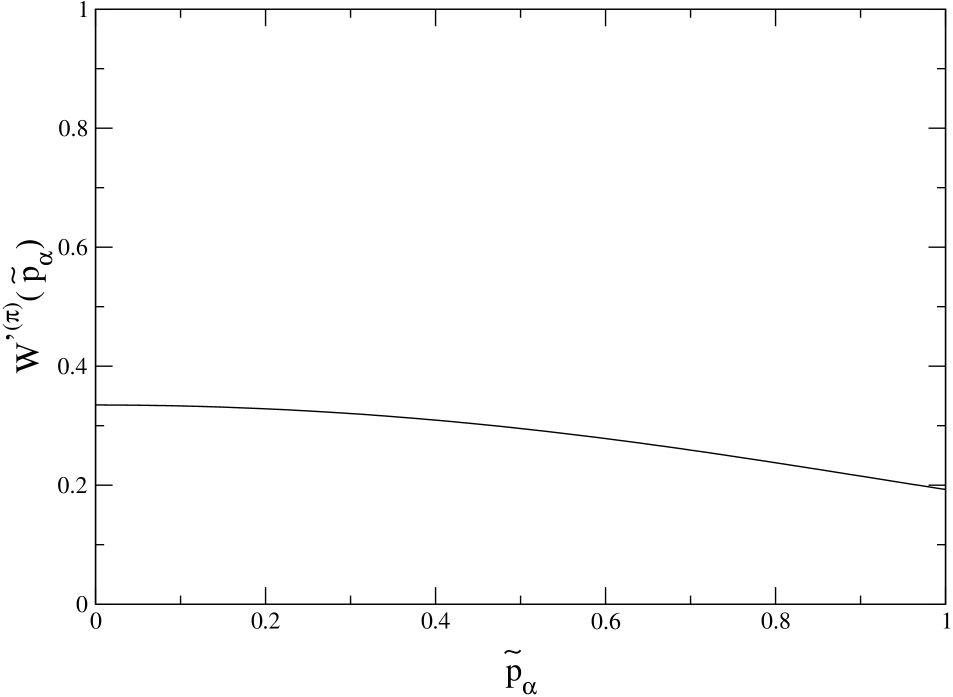
FIG. 10.: The smoothness of $W^{{}^{\prime}(\pi)}$ as a function of $\tilde{p}_{\alpha}$

Combining the spatial result with the spin and isospin factors from the tables the yields the $\pi$ pair current one-body averged form

$$j_{\gamma-PC}^{\pi\,\,pair} = \frac{eg_{\pi NN}f_{\pi}}{8\sqrt{2}\pi M}((\theta_{p}+\theta_{n})-(\theta_{p}-\theta_{n})\tau_{3})\vec{\sigma}\frac{2\pi\rho}{m^{2}_{\pi}}\langle W^{{}^{\prime}(\pi)}\rangle\delta^{(3)}(\vec{x}-\vec{x}_{i})+(1\leftrightarrow 2)$$ (13)

$$= \frac{eg_{\pi NN}f_{\pi}}{2\sqrt{2}\pi Mm^{2}_{\pi}}((\theta_{n}+\theta_{n})+(\theta_{n}-\theta_{p})\tau_{3})\times\rho\langle W^{{}^{\prime}(\pi)}\rangle\vec{\sigma}\delta^{(3)}(\vec{x}-\vec{x}_{i}).$$ (14)

Other currents are similar, though generally more tedious.

IV One-body Fermi-Gas Averaged Current Operators

We list the relevant one-body Fermi gas averaged operators in momentum space,

$$\vec{j}^{\pi\,\,pair}_{\gamma-PC} = \frac{eg_{\pi NN}f_{\pi}}{2\sqrt{2}Mm^{2}_{\pi}}((\theta_{n}+\theta_{p})+(\theta_{n}-\theta_{p})\tau_{3})\times\rho\langle W^{{}^{\prime}(\pi)}\rangle\vec{\sigma},$$ (1)

$$\vec{j}^{\rho\,\,pair}_{\gamma-PC} = \frac{2eg_{\rho NN}}{3Mm^{2}_{\rho}}(h^{1}_{\rho}+(h^{0}_{\rho}+\frac{h^{2}_{\rho}}{2\sqrt{6}})\tau_{3})\theta_{p}\rho\{\vec{\sigma}+\sqrt{\frac{15}{4}}\frac{1}{m^{2}_{\rho}}[[\vec{k}\otimes\vec{k}]_{2}\otimes\vec{\sigma}]_{1}\}$$ (2)

$$- \frac{g_{\rho NN}}{6Mm^{2}_{\rho}}\Bigg{(}\bigg{[}\Big{(}(h^{1}_{\rho}+\frac{3h^{2}_{\rho}}{2\sqrt{6}})+(2h^{0}_{\rho}+h^{1}_{\rho}+\frac{h^{2}_{\rho}}{2\sqrt{6}})\tau_{3}\Big{)}\theta_{p}-3(h^{0}_{\rho}-\frac{h^{2}_{\rho}}{2\sqrt{6}})(1+\tau_{3})\theta_{n}\bigg{]}2\rho\langle W^{{}^{\prime}(\rho)}\rangle\vec{\sigma}$$ (3)

$$+ \bigg{[}(3h^{0}_{\rho}+h^{1}_{\rho})-(h^{0}_{\rho}-h^{1}_{\rho}-\frac{2h^{2}_{\rho}}{\sqrt{6}})\tau_{3})\bigg{]}\theta_{n}\rho\sqrt{\frac{15}{4}}\langle W^{{}^{\prime\prime}(\rho)}\rangle\frac{1}{p^{2}_{F}}[[\vec{K}\otimes\vec{K}]_{2}\otimes\vec{\sigma}]_{1}\Bigg{)},$$ (4)

$$\vec{j}^{\rho\,\,pair}_{\gamma-PNC} = \frac{eg_{\rho NN}}{2Mm^{2}_{\rho}}(h^{0}_{\rho}+h^{1}_{\rho}+\frac{h^{2}_{\rho}}{2\sqrt{6}})(1+\tau_{3})(\theta_{n}-\theta_{p})\rho\vec{\sigma}$$ (5)

$$+ \frac{eg_{\rho NN}}{2Mm^{2}_{\rho}}\bigg{[}\Big{(}2h^{0}_{\rho}+h^{1}_{\rho}+\frac{h^{2}_{\rho}}{2\sqrt{6}}+(h^{1}_{\rho}+\frac{3h^{2}_{\rho}}{2\sqrt{6}})\tau_{3}\Big{)}\theta_{p}+(h^{0}_{\rho}-\frac{h^{2}_{\rho}}{2\sqrt{6}})(1+\tau_{3})\theta_{n}\bigg{]}\rho\langle W^{{}^{\prime}(\rho)}\rangle\vec{\sigma},$$ (6)

$$\vec{j}^{\omega\,\,pair}_{\gamma-PC} = \frac{2eg_{\omega NN}}{3Mm^{2}_{\omega}}(h^{0}_{\omega}+h^{1}_{\omega}\tau_{3})\theta_{p}\rho\{\vec{\sigma}+\sqrt{\frac{15}{4}}\frac{1}{m^{2}_{\omega}}[[\vec{k}\otimes\vec{k}]_{2}\otimes\vec{\sigma}]_{1}\}$$ (7)

$$- \frac{eg_{\omega NN}}{6Mm^{2}_{\omega}}(h^{0}_{\omega}+h^{1}_{\omega})(1+\tau_{3})\theta_{p}\ \rho\{2\langle W^{{}^{\prime}(\omega)}\rangle\vec{\sigma}\ -\sqrt{\frac{15}{4}}\langle W^{{}^{\prime\prime}(\omega)}\rangle\frac{1}{p^{2}_{F}}[[\vec{K}\otimes\vec{K}]_{2}\otimes\vec{\sigma}]_{1}\},$$ (8)

$$\vec{j}^{\omega\,\,pair}_{\gamma-PNC} = \frac{-eg_{\omega NN}}{2Mm^{2}_{\omega}}(h^{0}_{\omega}+h^{1}_{\omega})(1+\tau_{3})((\theta_{n}+\theta_{p})\ \rho\vec{\sigma}-\theta_{p}\ \rho\langle W^{{}^{\prime}(\omega)}\rangle\vec{\sigma}),$$ (9)

$$\vec{j}^{\pi\pi\gamma} = \frac{-eg_{\pi NN}f_{\pi}}{\sqrt{2}Mm^{4}_{\pi}}((\theta_{n}+\theta_{p})+(\theta_{n}-\theta_{p})\tau_{3})\ \rho\{\langle Y_{1}\rangle(\vec{\sigma}\cdot\vec{k})\vec{k}+\langle Y_{2}\rangle(\vec{\sigma}\cdot\vec{K})\vec{K}+\langle Y_{3}\rangle(p^{2}_{F})\vec{\sigma}\},$$ (10)

$$\vec{j}^{\rho\rho\gamma} = \frac{-eg_{\rho NN}}{2\sqrt{2}Mm^{4}_{\rho}}(h^{0}_{\rho}-\frac{h^{2}_{\rho}}{2\sqrt{6}})((\theta_{n}-\theta_{p})+(\theta_{n}+\theta_{p})\tau_{3})\ \rho\bigg{\{}\langle I_{1}\rangle(\vec{k}^{2})\vec{\sigma}+\langle I_{2}\rangle(p^{2}_{F})\vec{\sigma}$$ (11)

$$+ \langle I_{3}\rangle(\vec{\sigma}\cdot\vec{k})\vec{k}+\langle I_{4}\rangle(\vec{\sigma}\cdot\vec{K})\vec{K}-i\langle I_{5}\rangle\vec{k}\times\vec{K}+\frac{1}{m^{2}_{\rho}}\Big{(}\langle J_{1}\rangle(\vec{k}^{4})\vec{\sigma}+\langle J_{2}\rangle(\vec{k}\cdot\vec{K})^{2}\vec{\sigma}$$ (12)

$$+ \langle J_{3}\rangle(p^{2}_{F}\vec{k}^{2})\vec{\sigma}+\langle J_{4}\rangle(p^{4}_{F})\vec{\sigma}+\langle J_{5}\rangle(\vec{\sigma}\cdot\vec{k})(\vec{k}^{2})\vec{k}+\langle J_{6}\rangle(\vec{\sigma}\cdot\vec{K})(\vec{k}\cdot\vec{K})\vec{k}$$ (13)

$$+ \langle J_{7}\rangle(p^{2}_{F})(\vec{\sigma}\cdot\vec{k})\vec{k}+\langle J_{8}\rangle(\vec{\sigma}\cdot\vec{K})(\vec{k}^{2})\vec{K}+\langle J_{9}\rangle(p^{2}_{F})(\vec{\sigma}\cdot\vec{K})\vec{K}+\langle J_{10}\rangle(\vec{\sigma}\cdot\vec{k})(\vec{k}\cdot\vec{K})\vec{K}$$ (14)

$$- i\langle J_{11}\rangle(\vec{k}^{2})\vec{k}\times\vec{K}-i\langle J_{12}\rangle(p^{2}_{F})\vec{k}\times\vec{K}\Big{)}\bigg{\}},$$ (15)

$$\vec{j}_{\rho-PC}^{\rho\pi\gamma} = \frac{-i2\sqrt{2}eg_{\rho NN}f_{\pi}g_{\rho\pi\gamma}}{m_{\rho}(m^{2}_{\rho}+m^{2}_{\pi})^{2}}((\theta_{n}-\theta_{p})+(\theta_{n}+\theta_{p})\tau_{3})\ \langle Z\rangle\vec{k}\times\vec{K}.$$ (16)

$\theta_{p(n)}$ is a projection operator: when $\theta_{p(n)}$ acts on {$\rho$ (nuclear density), $p_{F}$ (Fermi momentum), $\langle X\rangle$ (averaged weighting function such as $\langle W^{{}^{\prime}(\pi)}\rangle$)}, the results should read {$\rho_{p(n)}$, $p^{p(n)}_{F}$, $\langle X_{p(n)}\rangle$}. The conversion rules from momentum space to position space are simple,

$$1 \longrightarrow \delta^{(3)}(\vec{x}-\vec{x}_{i}),$$ (17)

$$\vec{k}=\vec{p}_{\beta}-\vec{p}_{\alpha} \longrightarrow -i[\vec{\nabla},\delta^{(3)}(\vec{x}-\vec{x}_{i})],$$ (18)

$$\vec{K}=\frac{\vec{p}_{\beta}+\vec{p}_{\alpha}}{2} \longrightarrow -i\{\vec{\nabla}_{i},\delta^{(3)}(\vec{x}-\vec{x}_{i})\}_{sym}.$$ (19)

For ¹³³Cs, $p^{p(n)}_{F}\sim 260(300)$ MeV. The average weighting factors are given in Table XIX. For ²⁰⁵Tl, these numbers are almost the same. We do not distinguish between the $\rho$ and $\omega$ masses in evaluating weighting functions.

TABLE XIX.: Average weighting functions. (Note: First number refers to proton part and the the second the neutron part)

$\langle W^{{}^{\prime}(\pi)}\rangle$	$\langle W^{{}^{\prime}(\rho,\omega)}\rangle$	$\langle W^{{}^{\prime\prime}(\pi)}\rangle$	$\langle W^{{}^{\prime\prime}(\rho,\omega)}\rangle$	$\langle Y_{1}\rangle$	$\langle Y_{2}\rangle$	$\langle Y_{3}\rangle$
$0.30/0.26$	$0.90/0.88$	$0.99/1.02$	$0.19/0.23$	$0.0039/0.0033$	$0.0173/0.0111$	$0.0144/0.0103$
$\langle I_{1}\rangle$	$\langle I_{2}\rangle$	$\langle I_{3}\rangle$	$\langle I_{4}\rangle$	$\langle I_{5}\rangle$	$\langle J_{1}\rangle$	$\langle J_{2}\rangle$
$2.25/2.18$	$10.09/9.58$	$-1.53/-1.46$	$21.30/19.61$	$10.18/9.56$	$0.42/0.39$	$1.10/1.02$
$\langle J_{3}\rangle$	$\langle J_{4}\rangle$	$\langle J_{5}\rangle$	$\langle J_{6}\rangle$	$\langle J_{7}\rangle$	$\langle J_{8}\rangle$	$\langle J_{9}\rangle$
$4.11/3.91$	$1.43/1.32$	$-0.83/-0.77$	$-2.68/-2.48$	$2.57/2.40$	$4.25/3.89$	$-8.21/-7.56$
$\langle J_{10}\rangle$	$\langle J_{11}\rangle$	$\langle J_{12}\rangle$	$\langle Z\rangle$
$2.53/2.32$	$3.26/3.03$	$-11.16/-10.42$	$1.43/1.15$

REFERENCES

• [1] Ya. B. Zeldovich, Sov. Phys. JETP 6, 1184 (1958) and citation therein
• [2] E. M. Henley, A. Huffman, and D. Yu, Phys. Rev. D 7, 943 (1973)
• [3] V. V. Flambaum and I. B. Khriplovich, Sov. Phys. JETP 52, 835 (1980); V. V. Flambaum, I. B. Khriplovich, and O. P. Sushkov, Phys. Lett. B146, 367 (1984)
• [4] C. S. Wood, S. C. Bennett, D. Cho, B. P. Masterson, J. L. Roberts, C. E. Tanner, and C. E. Wieman, Science 275, 1759 (1997)
• [5] For more details, see e.g. E. G. Adelberger and W. C. Haxton, Annu. Rev. Nucl. Part. Sci. 35, 501 (1985); W. Haeberli and B. R. Holstein, “Symmetries and Fundamental Interactions in Nuclei”, ed. W. C. Haxton and E. M. Henley (World Scientific, Singapore, 1996)
• [6] B. Desplanques, J. Donoghue, and B. R, Holstein, Ann. Phys 124, 449 (1980)
• [7] P. Vetter, D. M. Meekhof, P. K. Majumder, S. K. Lamoreaux, and E. N. Fortson, Phys. Rev. Lett. B74, 2658 (1995)
• [8] N. H. Edwards, S. J. Phipp, P. E. G. Baird, and S. Nakayama, Phys. Rev. Lett. 74. 2654 (1995)
• [9] W. C. Haxton, E. M. Henley, and M. J. Musolf, Phys. Rev. Lett. 63, 949 (1989); W. C. Haxton, Science 275, 1753 (1997) and Nucl. Phys. A654, 315 (1999)
• [10] W. C. Haxton, C.-P. Liu, M. J. Ramsey-Musolf, Phys. Rev. Lett. 86, 5347 (2001)
• [11] C. Bouchiat and C. A. Piketty, Z. Phys. C49, 91 (1991) and Phys. Lett. B269, 195 (1991)
• [12] V. D. Dmitriev, I. B. Khriplovich, and V. B. Telitsin, Nucl. Phys. A577, 691 (1984)
• [13] V. D. Dmitriev and V. B. Telitsin, Nucl. Phys. A613, 237 (1997); V. D. Dmitriev and V. B. Telitsin, nucl-th/9912004
• [14] W. S. Wilburn and J. D. Bowman, Phys. Rev. C57, 3425 (1998)
• [15] N. Auerbach and B. A. Brown, nucl-th/9903032
• [16] I. B. Khriplovich, “Parity Nonconservation in Atomic Phenomena” (Gordon and Breach, Philadelphia, 1991)
• [17] R. R. Lewis, Comm. At. Mol. Phys. 31, 67 (1995)
• [18] See e.g. J. D. Jackson, “Classical Electrodynamics” (Wiley, New York, 1975)
• [19] V. V. Flambaum and D. W. Murray, Phys. Rev. C56, 1641, (1997)
• [20] See e.g. T. DeForest Jr. and J. D. Walecka, Ann. Phys. 15, 1 (1966)
• [21] A. J. F. Siegert, Phys. Rev. 52, 787 (1937)
• [22] J. L. Friar and W. C. Haxton, Phys. Rev. C31, 2027 (1985)
• [23] J. L. Friar and S. Fallieros, Phys. Rev. C29, 1654 (1984)
• [24] F. C. Michel, Phys. Rev. B133, 329 (1964)
• [25] For more details, see e.g., E. D. Commins and P. H. Bucksbaum, “Weak Interaction of Leptons and Quarks” (Cambridge Univ. Press, Cambridge, 1983); B. R. Holstein, “Weak Interactions in Nuclei” (Princeton Univ. Press, Princeton, 1989)
• [26] G. Barton, Nuovo Cimento 19, 512 (1961)
• [27] B. H. J. McKellar and P. Pick, Phys. Rev. D6, 2184 (1972); D7, 260 (1973)
• [28] V. M. Dubovik and S. V. Zenkin, Ann. Phys. 172, 100 (1986)
• [29] G. B. Feldman, G. A. Crawford, J. Dubach, and B. R. Holstein, Phys. Rev. C43, 863 (1991)
• [30] N. Kaiser and U.-G. Meissner, Nucl. Phys A510, 759 (1990); U.-G. Meissner and H. Weigel, Phys. Lett. B447, 1 (1999)
• [31] E. M. Henley, W.-Y. Hwang, and L. Kisslinger, Phys. Lett. B367, 21 (1996) and 440, 449(E) (1998)
• [32] S.-L. Zhu, S. J. Puglia, B. R. Holstein, and M. J. Ramsey-Musolf, Phys. Rev. D63, 033006 (2001)
• [33] M. J. Musolf and B. R. Holstein, Phys. Lett. B242, 461 (1990) and Phys. Rev. D43, 2956 (1991)
• [34] D. B. Kaplan and M. J. Savage, Nucl. Phys. A556, 653 (1993)
• [35] S.-L. Zhu, S. J. Puglia, B. R. Holstein, and M. J. Ramsey-Musolf, Phys. Rev. D62, 033008 (2000)
• [36] C. M. Maekawa and U. van Kolck, Phys. Lett. B478, 73 (2000)
• [37] W. C. Haxton and E. M. Henley, Phys. Rev. Lett. 51, 1937 (1983); V. V. Flambaum, Phys. Rev. A 60, R2611 (1999); J. Engle, J. L. Friar, and A. C. Hayes. Phys. Rev. C 61, 035502 (2000); A. Tsvetkov, J. Kvasil, and R. G. Nazmitdinov, nucl-th/0009085/
• [38] W. T. Baldridge and J. P. Vary, Phys. Rev. C14, 2246 (1976)
• [39] F. Nowacki, private communication
• [40] G. A. Miller and J. E. Spencer, Ann. Phys. 100, 562 (1976)
• [41] B. R. Berman, R. L. Bramblett, J. T. Caldwell, H. S. Davis, M. A. Kelly, and S. C. Fultz, Phys. Rev. 177, 1745 (1969); A. Lepretre, H. Beil, R. Bergere, P. Carlos, A. Deminiac, and A. Veyssiere, Nucl. Phys. A219, 39 (1974)
• [42] M. A. Bouchiat and C. Bouchiat, Phys. Lett. B48, 111 (1974), J. Physique 35, 899 (1974), J. Physique 36, 793 (1975), and Rep. Prog. Phys. 60, 1351 (1997); P. G. H. Sandars, Phys. Scripta 36, 904 (1987)
• [43] J. Erler and P. Langacker, Phys. Rev. Lett. 84, 212 (1990)
• [44] M. J. Ramsey-Musolf, Phys. Rev. C 60, 015501 (1999)
• [45] W. C. Haxton and C. E. Wieman, to appear in Ann. Rev. Nucl. Part. Sci. (nucl-th/0104026/)
• [46] R. Balzer, et al., Phys. Rev. C 30, 1409 (1984) and Phys. Rev. Lett. 44, 699 (1980)
• [47] J. M. Potter, et al., Phys. Rev. Lett. 33, 1307 (1974); D. E. Nagle, et al., 3rd International Symposium on High Energy Physics with Polarized Beams and Polarized Targets, AIP Conf. Proc. 51 (1978)
• [48] W. D. Ramsay, et al., Phys. Canada 55, 79 (1999)
• [49] J. Lang et al., Phys. Rev. Lett. 54, 170 (1985)
• [50] C. A. Barnes et al., Phys. Rev. Lett. 40, 840 (1978); P. G. Bizetti, et al. Lett. Nuovo Cimento 29, 167 (1982); G. Ahrens, et al. Nucl. Phys. A 390, 496 (1982); S. A. Page, et al., Phys. Rev. C 35, 1119 (1987) and Phys. Rev. Lett. 55, 791 (1985); A. R. Berdoz et al., submitted to Phys. Rev. Lett. (nucl-ex/0107014/); M. Bini, T. F. Fazzini, G. Poggi, and N. Taccetti, Phys. Rev. Lett. 55, 795 (1985)
• [51] E. G. Adelberger, et al., Phys. Rev. C 27, 2833 (1987); K. Elsener, et al., Nucl. Phys. A 461, 579 (1987) and Phys. Rev. Lett. 52, 1476 (1984)
• [52] W. C. Haxton, Phys. Rev. Lett. 46, 698 (1981)
• [53] J. Engel, W. C. Haxton, and P. Vogel, Phys. Rev. C 46, 2153 (1992)
• [54] A. Arima, Prog. Part. Nucl. Phys. 1, 41 (1978); A. Arima, K. Shimizu, W. Bentz, and H. Hyuga, Adv. Nucl. Phys. 18, 1 (1987)
• [55] B. Heckel, private communication
• [56] W. M. Snow, et al., Nucl. Instrum. Meth. A440, 729 (2000)
• [57] R. Hasty et al., Science 290, 2117 (2000)
• [58] See e.g. J. D. Bjorken and S. D. Drell, “Relativistic Quantum Mechanics” (McGraw-Hill, New York, 1964) and “Relativistic Quantum Fields” (McGraw-Hill, New York, 1965)