Correlations and charge distributions of medium heavy nuclei

Marta Anguiano and Giampaolo Co’

Dipartimento di Fisica, Università di Lecce and I.N.F.N. sez. di Lecce,

I-73100 Lecce, Italy

The effects of long- and short-range correlations on the charge distributions of some medium and heavy nuclei are investigated. The long-range correlations are treated within the Random Phase Approximation framework and the short-range correlations with a model inspired to the Correlation Basis Function theory. The two type of correlations produce effects of the same order of magnitude. A comparison with the empirical charge distribution difference between ²⁰⁶Pb and ²⁰⁵Tl shows the need of including both correlations to obtain a good description of the data.

PACS numbers: 21.10.Ft, 21.60.-n

1 Introduction

The high precision of modern electron scattering experiments imposes severe constraints to nuclear models and theories. The study of the charge density distributions of medium and heavy nuclei by means of elastic electron scattering has allowed for a detail test of the capacities of the independent particle model (IPM) to describe the nuclear ground state [1].

In the IPM the motion of each nucleon inside the nucleus is not affected by the presence of the other nucleons. The corrections beyond this picture take the generic name of correlations. The sources of correlations can be generically classified in two categories. The so called short-range correlations (SRC) are generated by the hard core repulsion of the nucleon-nucleon interaction which prohibits two nucleons to come too close to each other. The long-range correlations (LRC) are produced by collective excitation modes of the nucleus originated by the part of the nuclear hamiltonian neglected by the IPM.

This separation in long- and short-range correlation is an artifact of our approach to nuclear structure usually starting from an IPM basis. Exact solutions of the many-body Schrödinger equation, [2, 3] take automatically into account both kinds of correlations independently from their classification. When approximate or effective theories are used, the role of one or the other kind of correlation can be emphasized. The results recently obtained with Fermi Hypernetted Chain (FHNC) techniques in doubly magic nuclei shows the lack of some correlation effects [4, 5, 6], probably LRC. The aim of this article is to estimate the size of the effects of both kind of correlations on the charge density distributions of some medium and heavy nuclei.

We estimate the LRC within a Random Phase Approximation (RPA) approach, and the SRC effects by using a first order expansion model based on the Correlated Basis Function (CBF) theory. We analyze both the quantitative and qualitative differences between the effects of the two types of correlations. The inclusion of both of them is necessary to describe the charge distribution difference between ²⁰⁶Pb and ²⁰⁵Tl. The main message of our work is that, in medium heavy nuclei, the two kind of correlations produce equally important effects beyond the IPM.

The plan of the work is the following one. We briefly present in sects. 2 and 3 the theoretical background of our treatment of the correlations. In sect. 4 we first make a detailed description of the inputs of our calculations, then we present our results on the charge distributions of ¹⁶O, ⁴⁰Ca and ²⁰⁸Pb. At the end of the section we show our results regarding the charge distribution differences between the above mentioned nuclei and their isotone partners with one proton less. Finally we calculate the charge density difference between the open shell nuclei ²⁰⁶Pb and ²⁰⁵Tl and we compare it with the empirical one. In sect. 5 we summarize our work and draw our conclusions.

2 Long Range Correlations

The RPA many-body states are defined as:

$$|\Psi_{N}(RPA)>=Q^{\dagger}_{N}|\Psi_{0}(RPA)>$$ (1)

$$Q_{N}|\Psi_{0}(RPA)>=0$$ (2)

and the operator $Q_{N}$ satisfies the equations of motions

$$<\Psi_{0}(RPA)|\left[\delta Q_{N},\left[H,Q^{\dagger}_{N}\right]\right]|\Psi_{0}(RPA)>=\omega_{N}<\Psi_{0}(RPA)|\left[\delta Q_{N},Q^{\dagger}_{N}\right]|\Psi_{0}(RPA)>$$ (3)

for all the possible variations $\delta Q_{N}$. In the above equations we have indicated with $H$ the nuclear hamiltonian, with $[,]$ the commutator and with $\omega_{N}$ the excitation energy. The RPA theory uses:

$$Q^{\dagger}_{N}=\sum_{ph}X_{ph}(N)a^{\dagger}_{p}a_{h}-Y_{ph}(N)a^{\dagger}_{h}a_{p}$$ (4)

where $a^{\dagger}$ and $a$ are the creation and destruction operators respectively. The $X_{ph}(N)$ and $Y_{ph}(N)$ amplitudes are real numbers and are obtained by solving the RPA equations.

We are interested in evaluating the mean value of one-body operators on the RPA ground state defined by eq. (2). In a second quantization language this can be written as:

$$<{\cal O}>=<\Psi_{0}(RPA)|\sum_{\mu\mu^{\prime}}<\mu|{\cal O}|\mu^{\prime}>a^{\dagger}_{\mu}a_{\mu^{\prime}}|\Psi_{0}(RPA)>$$ (5)

where we have indicated with $|\mu>$ a single particle (s.p.) wave function generated by the mean field basis. The matrix element $<\Psi_{0}(RPA)|a^{\dagger}_{\mu}a_{\mu^{\prime}}|\Psi_{0}(RPA)>$ is evaluated as described in references [7, 8] and we obtain the result:

$$<{\cal O}>=\sum_{h}<h|{\cal O}|h>\left[1-\frac{1}{2}\sum_{N}\sum_{p}|Y_{ph}(N)|^{2}\right]+\sum_{p}<p|{\cal O}|p>\left[\frac{1}{2}\sum_{N}\sum_{h}|Y_{ph}(N)|^{2}\right]$$ (6)

where we have indicated with $p$ and $h$ the particle and hole states respectively. The operator defining the occupation number of a s.p. state $\mu$ is:

$${\cal N}_{\mu}=\delta_{\alpha,\mu}$$ (7)

where $\alpha=p,h$ in the sums of eq. (6). The modifications of the occupation numbers produced by RPA correlations has been studied in reference [8]. In this reference also the contribution of higher order excitations has been evaluated by means of a Second RPA calculation.

We are interested in the charge operator:

$$Q({\bf r})=\sum_{i}\delta({\bf r}-{\bf r}_{i})\frac{1}{2}\left[1+\tau_{3}(i)\right]$$ (8)

with $\tau_{3}(i)=\pm 1$ if the particle $i$ is a proton or a neutron respectively.

All our calculations are done in a j-j coupled spherical basis. This means that the s.p. wave functions are expressed as:

$$\phi^{t}_{nljm}({\bf r})=R^{t}_{nlj}(r)\sum_{\mu,s}<l\mu\frac{1}{2}s|jm>Y_{l,\mu}(\widehat{r})\chi_{s}$$ (9)

where we have indicated with $<|>$ the Clebsch-Gordan coefficients, with $Y_{l,\mu}(\widehat{r})$ the spherical harmonics, with $\chi_{s}$ the spin wave function and with $t$ the third component of the isospin.

Using the angular momentum coupled RPA equations and the expression (9) for the s.p. states, we obtain the following expression for the charge density distribution of a doubly-closed shell nucleus:

$$4\pi\rho_{LRC}(r) = \sum_{(nlj)h}(2j_{h}+1)(R_{(nlj)h}(r))^{2}\left[1-\frac{1}{2}\,\frac{1}{2j_{h}+1}\sum_{p}\sum_{J,N}(2J+1)|Y_{ph}(J,N)|^{2}\right]$$ (10)

$$+ \sum_{(nlj)p}(2j_{p}+1)(R_{(nlj)p}(r))^{2}\left[\frac{1}{2}\,\frac{1}{2j_{p}+1}\sum_{h}\sum_{J,N}(2J+1)|Y_{ph}(J,N)|^{2}\right]$$

where $p$ and $h$ indicate particle and hole states respectively limiting the range of the sums. In our calculations the sums on $p$ and $h$ are restricted only to proton states. We neglect the contribution of the neutrons to the charge distribution. In the IPM the $Y_{ph}(J,N)$ amplitudes are zero and eq. (10) gives the well known expression of $\rho_{IPM}$.

In this article we calculate also the charge distributions of nuclei with one proton less than the doubly magic ones. This is done within Landau-Migdal theory [9] which allows to calculate the difference between expectation values of operators in doubly magic nuclei and nuclei with one nucleon less (or more). The formalism has been widely used to calculate magnetic moments of nuclei around ²⁰⁸Pb [10] and it has been extended in references [11, 12] to the calculation of the charge distributions. The basic equation to be used to evaluate this difference is:

$$<A|{\cal O}_{J}|A>-<A-1;i|{\cal O}_{J}|k;A-1>=<i||{\cal O}_{J}||k>$$ (11)

$$+\sum_{N}\sum_{p_{1}p_{2}h_{1}h_{2}}<ip_{1}||V||kh_{1}>\frac{X_{p_{1}h_{1}}(J,N)X^{*}_{p_{2}h_{2}}(J,N)}{\epsilon_{p_{1}}-\epsilon_{h_{1}}-\omega_{N}}<p_{2}||{\cal O}_{J}||h_{2}>$$

$$-\sum_{N}\sum_{p_{1}p_{2}h_{1}h_{2}}<ip_{1}||V||kh_{1}>\frac{Y_{p_{1}h_{1}}(J,N)Y^{*}_{p_{2}h_{2}}(J,N)}{\epsilon_{p_{1}}+\epsilon_{h_{1}}-\omega_{N}}<h_{2}||{\cal O}_{J}||p_{2}>$$

In the above equation $V$ indicates the residual interaction used in RPA calculations, $\epsilon$ the s.p. energy, $\omega_{N}$ the RPA excitation energy of the N-th state and $|i>$ and $|k>$ the s.p. states characterizing the transition in the A-1 system within the IPM. To calculate the difference between ground state charge distribution we consider $J$=0 and the fact that $|i>$ = $|k>$ is the last occupied proton s.p. level just below the Fermi surface.

3 Short Range Correlations

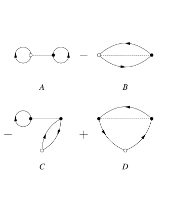
Figure 1: Cluster diagrams contributing to the one-body density. The dashed lines represent the dynamical correlations, $h^{p}$, and the oriented lines the statistical correlations, $\rho_{0}({\bf r}_{i},{\bf r}_{j})$. A black dot associated with a point implies integration over its coordinates.

We evaluate the effects of SRC on the ground state charge distribution by using the approach of references [13, 14]. The starting point is the following ansatz on the ground state:

$$\Psi_{0}(1,2...A)=G(1,2...A)\Phi_{0}(1,2...A)$$ (12)

where we have indicated with $\Phi_{0}$ the Slater determinant of s.p. states. The correlation operator is written as a symmetrized product of two-body operators:

$$G(1,2...A)={\cal S}\left[\prod_{i<j}F_{ij}\right]$$ (13)

The expression of $F_{ij}$ used in the most sophisticated calculations, both in nuclear matter and in finite nuclear systems, $F_{ij}$ has the form:

$$F_{ij}=\sum_{p=1,6}f^{p}(r_{ij})O^{p}_{ij}$$ (14)

where

$$O^{p=1,6}_{ij}=\left[1,\mbox{\boldmath$\sigma$}_{i}\cdot\mbox{\boldmath$\sigma$}_{j},S_{ij},\right]\otimes\left[1,\mbox{\boldmath$\tau$}_{i}\cdot\mbox{\boldmath$\tau$}_{j}\right]$$ (15)

In the above equations we have indicated with $S_{ij}=(3\,{\hat{\bf r}}_{ij}\cdot\mbox{\boldmath$\sigma$}_{i}\,{\hat{\bf r}}_{ij}\cdot\mbox{\boldmath$\sigma$}_{j}-\mbox{\boldmath$\sigma$}_{i}\cdot\mbox{\boldmath$\sigma$}_{j})$ the tensor operator.

The expectation value of a generic operator ${\cal O}$ is:

$$<{\cal O}>=\frac{<\Psi_{0}|{\cal O}|\Psi_{0}>}{<\Psi_{0}|\Psi_{0}>}$$ (16)

In CBF theory the ground state is found through the minimization of the hamiltonian expectation value. The search for this minimum involves variations on the parameters of the correlation functions $f^{p}$ and of the mean field potential defining the s.p. basis.

The charge distribution is obtained by inserting in eq.(16) the charge density operator (8). We found convenient to rewrite the correlation function (13) as:

$$G(1,2...A)=1+{\cal S}\prod_{i<j}\left[\sum_{p=1,6}h^{p}(r_{ij})O^{p}_{ij}\right]\,.$$ (17)

where we have defined $h^{1}=f^{1}-1$ and $h^{p>1}=f^{p>1}$. The expectation value is evaluated with standard cluster expansions techniques [15] which allow us to express it as infinite sum of linked diagrams. The unlinked terms of the numerators are canceled by the denominator.

At this point we introduce an approximation. We evaluate only those diagrams containing a single correlation function $h^{p}$. The diagrams considered are shown in figure 1. It is evident from Eq. (17) that the first term of our calculation is the IPM density which is already properly normalized. This implies that in the normalization procedure the contribution of all the correlation diagrams should vanish. It is shown in reference [13] that the set of diagrams of figure 1 provides the correct normalization of the density.

The validity of our approximation in calculating the charge distribution has been studied in reference [13] by comparing the results of the model with those of a Fermi Hypernetted Chain calculation. A test of the approximation in the evaluation of the nuclear matter charge responses has been done in reference [16]. More recently [6] the approximation has been tested in the evaluation of the one-body densities and the natural orbits. The conclusion of these investigations is that the approximation is reliable. This is probably related to the fact that the charge operator is a relatively simple one-body operator, therefore not very sensitive to the fine details of the many-body wave function.

The calculation of the correlated density is carried on by expanding the correlation function (17) in terms of Legendre polynomials. This facilitates the calculation in the spherical basis of the s.p. wave functions (9). Details are given in reference [13].

4 Applications

4.1 The input

We have conducted our study in three different mass regions located around the doubly magic nuclei ¹⁶O, ⁴⁰Ca and ²⁰⁸Pb. In our calculations we used the same set of s.p. wavefunctions for evaluating both LRC and SRC effects. These wavefunctions have been generated by diagonalizing a Woods–Saxon potential in a harmonic oscillator basis. This procedure automatically discretizes the continuum. In the RPA calculations we used configuration spaces considering all the states below the Fermi surface and three major shells above it. We found good convergence of our calculations when multipole excitations up to J=10 were used.

	$f^{in}$	$f^{ex}$	$f^{\prime in}$	$f^{\prime ex}$	$g_{0}$	$g^{\prime}_{0}$
$V_{LM}$	0.20	-2.45	1.50	1.50	0.55	0.70
$V_{JS}$	0.21	-1.80	0.65	1.65	0.70	0.70

Table 1: Parameters of the Landau-Migdal force, $V_{LM}$, and of the zero–range part of the Jülich-Stony Brook interaction $V_{JS}$. We used the same normalization constant $C_{0}$ for both interaction. For ¹⁶O and ²⁰⁸Pb calculations we used $C_{0}$=386 MeV fm³, while for ⁴⁰Ca $C_{0}$=212 MeV fm³. The density dependent parameters have been changed for each nucleus considered. They are $\alpha$=0.50, 0.53, 0.60 fm^-1 and $R_{F}$= 3.0, 4.1, 7.22 fm respectively for ¹⁶O, ⁴⁰Ca and ²⁰⁸Pb.

The parameters of the potential we have adopted are taken form the literature [17, 18] and have also been used in the FHNC calculations of reference [19], where j-j coupling and isospin dependence of the s.p. wave functions were considered. We obtained the charge distribution by folding the pointlike proton distributions with the nucleon electromagnetic form factors of reference[20].

The RPA calculations used to evaluate the LRC effects require an additional input: the particle-hole interaction. We have tested the sensitivity of our results to the choice of this input by using two different types of interaction. A first one is a Landau-Migdal (LM) contact interaction of the form:

$$V_{LM}({\bf r}_{1},{\bf r}_{2})=C_{0}\left[f_{0}(r_{1})+f^{\prime}_{0}(r_{1})\mbox{\boldmath$\tau$}_{1}\cdot\mbox{\boldmath$\tau$}_{2}+g_{0}(\rho)\mbox{\boldmath$\sigma$}_{1}\cdot\mbox{\boldmath$\sigma$}_{2}+g^{\prime}_{0}(\rho)\mbox{\boldmath$\sigma$}_{1}\cdot\mbox{\boldmath$\sigma$}_{2}\mbox{\boldmath$\tau$}_{1}\cdot\mbox{\boldmath$\tau$}_{2}\right]\delta^{3}({\bf r}_{1}-{\bf r}_{2})$$ (18)

The experience of RPA calculations in the Pb region [10] has shown the need of imposing a density dependence to the scalar and isospin parameters $f_{0}$ and $f^{\prime}_{0}$ parameters. As suggested in reference [17] for these two channels we use the expression:

$$f(r)=f^{ex}+(f^{in}-f^{ex})\frac{1}{1+exp[\alpha(r-R_{F})]}$$ (19)

where $\alpha$ and $R_{F}$ are two free parameters. The factor $C_{0}$ represents the inverse of the density of states at the Fermi surface and we consider it as a free parameter used to set the full strength of the force.

The second RPA interaction is the finite range Jülich–Stony Brook (JSB) force [21], obtained by adding to the zero range piece of Landau-Migdal type, the contribution of one-pion plus one-rho meson exchange potentials. This is a finite range interaction and in the discrete excitation spectrum is necessary to obtain a good description of the magnetic excitations [22].

The values of the parameters used in our calculations are given in table 1. The parameters of the delta interaction are those of reference [17] where have been fixed to reproduce the excitation energy of the low lying 2⁺ and 3^- states in ²⁰⁸Pb as well as the position of the the monopole giant resonance. We have adjusted the free parameters of the JSB force to reproduce the 3^- state of ²⁰⁸Pb at 2.61 MeV. We obtained for the $B(E3;0\rightarrow 3)$ values: $7.536\times 10^{5}$ e²fm⁶ with LM interaction and $7.489\times 10^{5}$ e²fm⁶ with JSB, in agreement with the experiment [23].

Even though the parameters of the two interactions have been tuned in the lead region their performances in reproducing the ¹⁶O spectrum are quite good. The low lying 3^- state of ¹⁶O was obtained at the energy of 6.95 MeV and at 7.35 MeV respectively for the LM and the JSB interactions. These values should be compared with the experimental values of 6.13 MeV. In this case the $B(E3;0\rightarrow 3)$ values are $0.97\times 10^{2}$ e²fm⁶ for LM and $1.17\times 10^{3}$ e²fm⁶ for JSB to be compared with the experimental value, $1.5\times 10^{3}$ e²fm⁶ [23]. This good result is obtained because the empirical single particle energies are rather well reproduced by the spherical Woods-Saxon potential.

The situation is rather different for ⁴⁰Ca. In this case the splitting between the single particle levels around the Fermi surface is narrower than the empirical one. For this reason the interaction fixed in ²⁰⁸Pb is too attractive. We got an imaginary eigenvalue for the first 3^- state. We reduced the value of $C_{0}$ from $386$ MeV fm³ down to $212$ MeV fm³ and we obtained for the 3^- the energies of 1.48 MeV and 3.20 MeV for LM and the JSB forces respectively. The experimental value is 3.73 MeV. The LM force gives a too low $B(E3;0\rightarrow 3)$ value, $1.1762\times 10^{4}$ e²fm⁶ (the experimental one is $1.70\times 10^{4}$ e²fm⁶ [23]), while the JSB gives $1.22\times 10^{4}$ e²fm⁶.

Figure 2: Differences between IPM charge densities and those obtained considering LRC correlations. The full lines have been obtained with the Jülich-Stony Brook interaction, the dashed lines with the Landau-Midgal force.

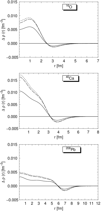
Figure 3: Differences between IPM densities and those obtained considering SRC correlations. The full lines have been obtained with the state dependent correlations of reference [4] and the long dashed lines by using only the central term of this correlation. The gaussian correlation of reference [19] produces the short dashed lines.

In figure 2 we show the differences between the IPM charge distributions and those calculated considering the LRC evaluated with the two interactions. We can see that the densities calculated with the Landau–Migdal and the Jülich-Stony Brook interactions are very similar. The differences between the results obtained with the two forces are within the accuracy of the data.

In our model, the input required to evaluate the SCR effects are the correlation functions of eq.(17). In variational calculations these functions, together with the s.p. wave functions, are determined by the minimization procedure. In the calculations of reference [19] where the semi-realistic nucleon-nucleon S3 interaction [24] has been used simple scalar correlation functions were required. In our calculations we have considered the gaussian correlations of reference [19]. Their expression is:

$$f^{(1)}(r)=1-A\exp(-Br^{2})$$ (20)

and the parameters $A$ and $B$ have been fixed by the minimization procedure. It has been shown in reference [19] that, for a fixed nucleon-nucleon interaction, the correlation functions are almost the same for every nucleus considered. The obtained values of the two parameters were $A$=0.7 and $B$=2.2 fm^-2. The differences between IPM charge distributions and those calculated with this correlation function are given by the short dashed-lines of figure 3.

We studied the effects of the state dependent terms of the correlation function by using the correlations defined by the FHNC calculations of reference [4]. In this reference the realistic V8’ nucleon-nucleon interaction plus the Urbana IX three-nucleon interaction [2] have been used. The difference between IPM charge distributions and those obtained with this correlation functions are presented in figure 3 by the full lines. We performed calculations switching off the state dependent part of the correlations and we used only the scalar part. The results of these calculations are given by the long dashed lines of figure 3. When the state dependent part of the correlation is switched off we essentially reproduce the curves obtained with the gaussian correlation. The contribution of the state dependent correlations diminish the difference with the IPM results. These results confirm the findings of references [6, 13, 14].

In the calculations we shall discuss in the next sub-sections we shall refer to the LRC calculations as those done with the Jülich–Stony Brook interaction and to the SRC as those done with the full state dependent correlation of reference [4].

4.2 Doubly magic nuclei

The IPM charge distributions of ¹⁶O, ⁴⁰Ca and ²⁰⁸Pb are compared in figure 4 with those obtained after the inclusion of the correlations. The effects produced by both kind of correlations are analogous. The charge distribution is lowered in the center of the nucleus and this implies an increase of the rms charge radii as it is shown in table 2.

	16O	40Ca	208Pb
IPM	2.64	3.25	5.46
SRC	2.70	3.31	5.52
LRC	2.98	3.57	5.59

Table 2: Root mean square charge radii in fm.

The correlations change the occupation probability of the s.p. states with respect to those of the IPM. For the LRC we calculated the occupation probabilities by evaluating the expectation values of the operator defined in Eq. (7). The results are shown in figure 5 where we observe that the main changes are around the Fermi surface.

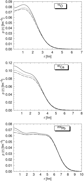
Figure 4: Charge density distributions for the three closed shell nuclei investigated. IPM (full lines), LRC (long dashed lines), SRC (short dashed lines).

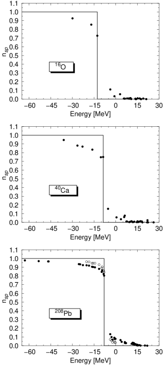
Figure 5: Proton occupation numbers as a function of the single particle energy. The full lines represent a Fermi gas distribution. The white dots in the lowest panel show the results of reference [25].

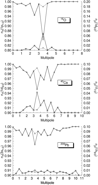
Figure 6: Occupation numbers of the valence hole and particle states as a function of the excitation multipole. On the abscissa the multipoles are odered for a fixed value of $J$ first with positive and then negative parity. The left vertical scales and the upper lines refer to the hole states and the right scales associated with the lower lines to the particle states. The dashed lines show the results obtained by leaving out the lowest collective 3^- states.

Our LRC correlations produce slightly stronger effects than those found by Gogny [25], whose results are shown by the white dots in the ²⁰⁸Pb panel of figure 5. Our LRC effects are strong also in comparison with those of the RPA calculations of reference [8] done in the ⁴⁰Ca nucleus. These differences are due to the different interactions and s.p. bases used.

In the LRC calculations the change of the occupation probability is due to the coupling of the s.p. level with the collective excitation of the nucleus. This is clearly shown in figure 6 where the occupation probabilities of the two s.p. levels just below and above the Fermi surface are shown as a function of the multipole excitation. It is evident that the occupation probability is strongly modified in correspondence to the 3^- states. The dashed lines show the result of a calculation when the lowest collective 3^- state is not considered.

The SRC correlations produce analogous effects on the occupation probabilities of the s.p. levels. An evaluation of these modifications is not straightforward as in the case of LRC since in the CBF calculations the quantities used are the one- and two-body densities and not the s.p. wave functions. We have calculated the one-body densities for the three nuclei considered within our first order correlation model by using the multipole decomposition technique described in references [13, 14]. We projected the $l$ multipole term $\rho_{l}(r_{1},r_{2})$ of the one-body density matrix on the s.p. basis by calculating

$$n_{SRC}=\int dr_{1}\,r^{2}_{1}\int dr_{2}\,r^{2}_{2}R_{nlj}(r_{1})R_{nlj}(r_{2})\rho_{l}(r_{1},r_{2})$$ (21)

The occupation numbers for the $s$ waves obtained with this procedure are compared in table 3 with the LRC ones. In our calculation the LRC are more effective in lowering the occupation probability of the valence states than the SRC.

	16O		40Ca		208Pb
	LRC	SRC	LRC	SRC	LRC	SRC
1s1/2	0.93	0.95	0.93	0.94	0.97	0.93
2s1/2			0.78	0.94	0.92	0.91
3s1/2					0.80	0.92

Table 3: Occupation probability of the $s$ states.

We obtained for the occupation probability of the 3s1/2 state of ²⁰⁸Pb the value of 0.74, which is slightly larger than the 0.6 extracted from the (e,e’p) data of ref. [26] even though recent DWBA re-analysis obtained a value of 0.7 [27]. The nuclear matter studies of SRC and LRC of the occupation probability predict values around 0.8 [28, 29]. As expected our value is lower than this since we also include surface vibrations.

4.3 Semi-magic nuclei

We have calculated the differences between the charge distributions of isotones differing by one proton only, since we expect this quantity to be less dependent from the choice of the s.p. wave functions than the full charge distribution. The results of these calculations for the three pairs of isotones considered are shown in figure 7. The IPM results correspond to the square of the s.p. wave function of the least bound proton state. They are the $1p_{1/2}$, $1d_{3/2}$ and $3s_{1/2}$ s.p. states for the ¹⁶O, ⁴⁰Ca and ²⁰⁸Pb nuclei respectively. The shape of the curves shown in the figure reproduce the known behaviour of these s.p. wave functions. Only the $s$ wave is peaked in the center of the nucleus, the other ones have their maxima at larger distances.

With respect to the IPM results, the correlations diminish the difference in the central part of the nucleus and tends to shift the charge in the external regions. In the ¹⁶O–¹⁵N and ⁴⁰Ca–³⁹K systems this effect produces a shift of the maxima. In the ²⁰⁸Pb–²⁰⁷Tl system the inclusion of the correlations lowers the difference in the center of the nucleus. As in the case of the doubly magic nuclei short and long range correlations produce effects of the same order of magnitude.

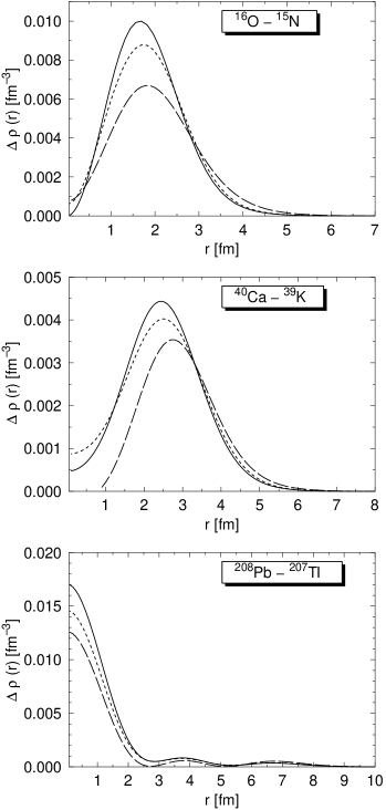
Figure 7: Charge distribution differences between isotones. IPM (full lines), SRC (short dashed lines) and LRC (long dashed lines).

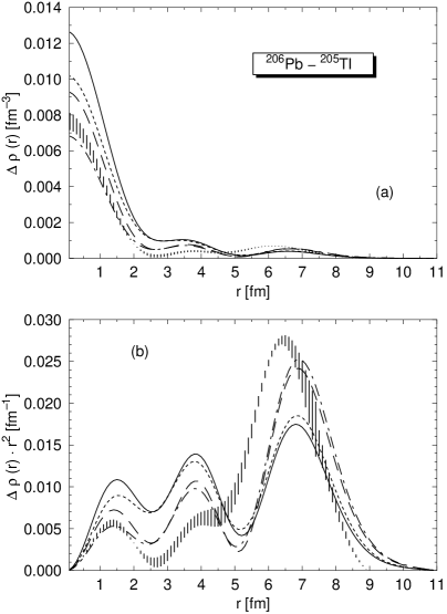
Figure 8: Differences between ²⁰⁶Pb and ²⁰⁵Tl charge densities. Full lines IPM, dotted lines SRC, dashed lines LRC, dashed dotted lines full calculation. In the lower panel the charge densities are multiplied by r² to emphasize the large distance behaviour. The experimental data are from [1, 30].

The interest in the calculation of these charge differences is related to the existence of experimental data in the lead region. In a single experiment [1, 30] the elastic electron scattering cross sections of ²⁰⁶Pb and ²⁰⁵Tl have been measured. From the analysis of these data the empirical difference between the charge distributions of these two nuclei has been extracted. In the center of the nucleus the IPM predicts a larger charge difference than the one deduced by the experimental data.

A direct comparison between the differences shown in the lowest panel of figure 7 and the experimental one is not correct since the ²⁰⁶Pb and ²⁰⁵Tl nuclei have a rich open shell structure which is not considered in the ²⁰⁸Pb and ²⁰⁷Tl system. To describe the two open shell nuclei we adopted the model already used in reference [12]. The ground state of ²⁰⁵Tl is described as:

$$|1/2^{+},^{205}{\rm Tl}> = \alpha_{1}(|3s_{1/2}>^{-1}\otimes\,|0^{+},^{206}{\rm Pb}>$$ (22)

$$+ \alpha_{2}(|2d_{3/2}>^{-1}\otimes\,|2^{+},^{206}{\rm Pb}>$$

$$+ \alpha_{3}(|2d_{5/2}>^{-1}\otimes\,|2^{+},^{206}{\rm Pb}>$$

where we considered $\alpha_{1}$=0.86, $\alpha_{2}$=-0.47, $\alpha_{3}$=0.30, obtained in reference [31] using first order perturbation theory with a $\delta$ interaction. The $0^{+}$ and $2^{+}$ states of the ²⁰⁶Pb are obtained as linear combination of two-hole wave functions in the closed neutron core of ²⁰⁸Pb [32]. We use the hole-hole amplitudes calculated in reference [33] within a Tamm–Dankoff Approximation. The ground state amplitudes are rather similar to those given in reference [23] which reproduce the empirical values obtained by an analysis of (d,p) reactions on ²⁰⁶Pb target. The IPM charge difference obtained with these wavefunctions is represented by the full lines of figure 8.

While the LRC have been consistently treated within the open shell structure of the two nuclei [12], this has not be done for the SRC. In this case we supposed their effect to be the same as that calculated in closed shell nuclei:

$$\rho_{\rm SRC}^{206}(r)\simeq\rho_{\rm SRC}^{208}(r)-[\rho_{\rm IPM}^{208}(r)-\rho_{\rm IPM}^{206}(r)]$$

and analogously for the 205–207 system. With this hypothesis the total charge difference between ²⁰⁶Pb and ²⁰⁵Tl is:

$$\Delta_{\rm TOT}^{206-205}(r)=\Delta_{\rm LRC}^{206-205}(r)+\Delta_{\rm SRC}^{206-205}(r)-\Delta_{\rm IPM}^{206-205}(r)\simeq\Delta_{\rm LRC}^{206-205}(r)+\Delta_{\rm SRC}^{208-207}(r)-\Delta_{\rm IPM}^{208-207}(r)$$

where we have indicated with $\Delta$ the difference between the charge densities of the two nuclei indicated in the upper index. The total difference evaluated in this way is compared in figure 8 with the empirical one. The inclusion of both long and short range correlations greatly improves the agreement with the experiment. In the lower panel we show the differences multiplied by $r^{2}$ to emphasize the comparison at large values of the nuclear radius. Also in this region the inclusion of both correlations improves the agreement.

5 Summary and Conclusions

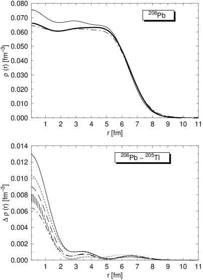
Figure 9: Results obtained with a new set of s.p. states (see text). Upper panel: ²⁰⁸Pb charge distributions compared with the empirical one [34] represented by the thick line. The thin full line show the IPM result, the dashed line has been obtained by summing long and short range correlations. Lower panel: Differences between ²⁰⁶Pb and ²⁰⁵Tl charge densities. The meaning of the lines is analogous to that of figure 8.

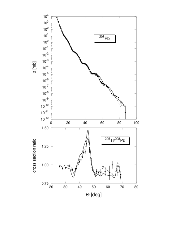
Figure 10: Above: elastic electron scattering cross section on ²⁰⁸Pb (data from [35]). Below: ratio beteen the elastic cross sections on ²⁰⁵Tl and ²⁰⁶Pb targets (data from [1]). The full lines represent the IPM results and the dashed-dottoed ones the results obtained includibg both LRC and SRC.

We have calculated the effects of long and short-range correlations on the charge distribution of some doubly magic nuclei. The SRC have been treated in the framework of the Correlated Basis Function theory. We use a first order model in the correlation function. The correlations have been taken from FHNC calculations done with realistic interaction. The LRC correlations have been treated within a RPA framework. In this case we used an effective interaction whose parameters have been fixed to reproduce the ²⁰⁸Pb low-energy excitation spectrum.

We have seen that long- and short- range correlations produce similar effects on the charge distributions. In both cases the IPM distributions are lowered in the center of the nucleus and, as a consequence, the rms radii increase. In terms of s.p. occupation numbers this effect is produced because both kinds of correlations decrease the occupation of the hole states and increase that of the particle states. We have shown that in all the nuclei considered the link between s.p. levels and collective low-lying 3^- state is one of the major sources of modification of the occupation number.

The charge differences with nuclei having one proton less have been calculated in order to compare our results with the measured empirical difference in the Pb region. Also on the charge difference the two kind of correlations produce similar results. Also in this case the correlations tend to diminish the difference in the central region. After a proper consideration of the open shell structure of the ²⁰⁶Pb and ²⁰⁵Tl nuclei, the total difference which considers both correlations can reproduce the empirical one.

Our calculations do not treat LRC and SRC on the same ground. A mixing of ingredients taken from fundamental theory, the correlation functions, and effective theory, the RPA correlations, has been used in our calculations. In all our work the choice of s.p. wave functions is essential. The sets of s.p. states we have used have been taken from the literature and the parameters of the mean field used to generate them have been fixed to reproduce at best the s.p. energies of the valence states around the Fermi level, and the charge distributions. For this reason we did not make a comparison between our charge distributions and the experimental ones. Since the IPM densities are already reproducing rather well the empirical ones, the inclusion of correlations worsen the agreement with the experiment.

It is sufficient a small change in the mean field parameters to obtain a set of s.p. states which can reproduce the empirical densities after the inclusion of the correlations. We have done that for ²⁰⁸Pb where we have changed the Woods-Saxon depth $V_{0}$ from 60.4 MeV to 62.0 MeV and the radius from 7.46 fm to 7.4 fm. The results obtained with this new set of s.p. wave functions are shown in figure 9. In the upper panel we compare ²⁰⁸Pb charge densities with the empirical one [34]. In the lower panel we show that even with the new set of s.p. states the charge density difference between ²⁰⁶Pb and ²⁰⁵Tl is well reproduced.

In the upper panel of figure 10 we compare with the data of ref. [35] the electron scattering elastic cross sections calculated within the Distorted Wave Born Approximation by using the densities of the previous figure. The dashed-dotted line obtained by including both SRC and LRC reproduces better the data than the IPM density (full line). In the lower panel we compare our results with the ratio of the elastic cross sections measured on ²⁰⁶Pb and ²⁰⁵Tl targets [1]. Also in this case the line better reproducing the data is the dashed-dotted one obtained by including all the correlation effects.

We have presented these results to show that we would be able to describe the empirical densities with small changes of the mean field parameters. This was not the goal of our work. We simply wanted to investigate the relative role played by long and short range correlations, and we found that they should be simultaneously considered in order to obtain a successful description of the empirical densities. This is our main message.

The facts triggering our investigation are related to the difficulties found by recent CBF variational calculations [4] in reproducing the experimental binding energies and charge distributions of some doubly closed shell nuclei. These microscopic calculations, depending only from the realistic nucleon-nucleon interaction, provide a good description of the SRC. Our work adds another piece of evidence that the adequate treatment of the LRC is the missing ingredient. Hopefully, perturbative corrections, like those developed in in references [36, 37] for nuclear matter, could provide the required description of the LRC.

Acknowlegments
We thank P.F. Bortignon and A.M. Lallena for useful discussions. This work has been partially supported by MURST through the Progetto di Ricerca di Interesse Nazionale: Fisica teorica del nucleo atomico e dei sistemi a molticorpi.

References

- [1] Cavedon J M et al 1982 Phys. Rev. Lett. 49 978
- [2] Pudliner B S, Pandharipande V R, Carlson J, Pieper S C and Wiringa R B 1997 Phys. Rev. C 56 2261
- [3] Wiringa R B, Pieper S C, Carlson J and Pandharipande V R 2000 Phys. Rev. C 62 0144001
- [4] Fabrocini A, Arias de Saavedra F and Co’ G 2000 Phys. Rev. C 61 044302
- [5] Mokhtar S R, Co’ G and Lallena A M 2000 Phys. Rev. C 62 067304
- [6] Fabrocini A and Co’ G 2001 Phys. Rev. C 63 044319
- [7] Rowe D J 1968 Phys. Rev. 175 1283
- [8] Lenske H. and Wambach J 1990 Phys. Lett. B 249 377
- [9] Migdal A B 1967 Theory of finite Fermi systems and applications to atomic nuclei (New York: John Wiley)
- [10] Speth J, Werner E and Wild W 1977 Phys. Rep. 33 127
- [11] Co’ G and Speth J 1986 Phys. Rev. Lett. 57 547
- [12] Co’ G and Speth J 1987 Zeit. Phys. A 326 361
- [13] Co’ G Nuov. Cim. 1995 A 108 623
- [14] Arias de Saavedra F, Co’ G and Renis M M 1997 Phys. Rev. C 55 673
-
[15]
Clark J W 1979 Prog. Part. and Nucl. Phys. 3 89
Pandharipande V R and Wiringa R B 1979 Rev. Mod. Phys. 51 821
S. Rosati 1982 From nuclei to particles, Proc. Int. School E. Fermi, course LXXIX ed. A. Molinari (Amsterdam: North Holland) pp 73-112 - [16] Amaro J E, Lallena A M, Co’ G and Fabrocini A 1998 Phys. Rev. C 57 3473
- [17] Rinker G A and Speth J 1978 Nucl. Phys. A 306 360
- [18] Co’ G, Lallena A M and Donnelly T W 1987 Nucl. Phys. A 469 684
- [19] Arias de Saavedra F, Co’ G, Fabrocini A and Fantoni S 1996 Nucl. Phys. A 605 359
- [20] Bertozzi W, Friar J, Heisenberg J and Negele J W 1972 Phys. Lett. B 41 408
- [21] Speth J, Klemt V, Wambach J and Brown G E 1980 Nucl. Phys. A 343 382
- [22] Co’ G and Lallena A M 1990 Nucl. Phys. A 510 139
- [23] A. Bohr and B. Mottelson 1975 Nuclear Structure, Vol. II (London: Benjamin) pp 561 and 642
- [24] Afnan I R and Tang Y C 1968 Phys. Rev. 175 1337
- [25] Gogny D 1979 Nuclear Physics with Electromagnetic Interactions, ed H. Arenhövel and D. Drechsel, Lecture Notes in Physics, Vol. 108 (Berlin: Springer) p 88
-
[26]
Quint E N M et al 1986
Phys. Rev. Lett. 57 186
Quint E N M et al 1987 Phys. Rev. Lett. 58 1088 - [27] Udías J M, Sarriguren P, Moya de Guerra E, Garrido E and Caballero J A 1993 Phys. Rev. C 48, 2731
- [28] Pandharipande V R, Papanicolas C N and Wmbach J 1984 Phys. Rev. Lett. 53, 1133
- [29] Benhar O, Fabrocini A and Fantoni S 1990 Phys. Rev. C 41, R24
- [30] Frois B et al 1983 Nucl. Phys. A A396 409c
- [31] Zamick L, Klemt V and Speth J 1985 Nucl. Phys. A 245 365
- [32] Klemt V and Speth J 1976 Zeit. Phys. A 278 59
- [33] Kuo T T S and Herling G H 1971 Naval Research Laboratory Memorandum Report 2258
- [34] De Jager C W and De Vries C 1987 At. Data Nucl. Data Tables 36 495
-
[35]
Heisenberg J et al 1969
Phys. Rev. Lett. 23 1402
Eutener M et al 1976 Phys. Rev. Lett. 36 129
Frois B et al 1977 Phys. Rev. Lett. 38 152 - [36] Fantoni S and Pandharipande V R Nucl. Phys. A 427 473
- [37] Benhar O, Fabrocini A and Fantoni S 1989 Nucl. Phys. A 505 267