Renormalization of equations governing nucleon
dynamics
and nonlocality in time of the NN interaction.
Abstract
We discuss the problem of renormalization of dynamical equations which arises in an effective field theory description of nuclear forces. By using a toy model of the separable NN potential leading to logarithmic singularities in the Born series, we show that renormalization gives rise to nucleon dynamics which is governed by a generalized dynamical equation with a nonlocal-in-time interaction operator. We show that this dynamical equation can open new possibilities for applying the EFT approach to the description of low-energy nucleon dynamics.
pacs:
21.45.+v, 02.70.-c, 24.10.-iI Introduction
Understanding how nuclear forces emerge from the fundamental theory of quantum chromodynamics (QCD) is one of the most important problem of quantum physics. To study hadron dynamics at scales where QCD is strongly coupled, it is useful to employ effective field theories (EFT’s) [1] being an invaluable tool for computing physical quantities in the theories with disparate energy scales. In order to describe low energy processes involving nucleons and pions, all possible interaction operators consistent with the symmetries of QCD are included in an effective Lagrangian of an EFT. However such a Lagrangian leads to ultraviolet (UV) divergences that must be regulated and a renormalization scheme defined. A fundamental difficulty in an EFT description of nuclear forces is that they are nonperturbative, so that an infinite series of Feynman diagrams must be summed. Summing the relevant diagrams is equivalent to solving a Schrödinger equation. However, an EFT yields graphs which are divergent, and gives rise to a singular Schrödinger potential. For this reason N-nucleon potentials are regulated and renormalized couplings are defined [2]. Nevertheless, a renormalization procedure does not lead to the potentials satisfying the requirements of ordinary quantum mechanics, and consequently after renormalization nucleon dynamics is not governed by the Schrödinger equation. This raises the question of what kind of equation governs nucleon dynamics at low energies. The Schrödinger equation is local in time, and the interaction Hamiltonian describes an instantaneous interaction. This is the main cause of infinities in the Hamiltonian formalism. In Ref.[3] it has been shown that the use of the Feynman approach to quantum theory [4] in combination with the canonical approach allows one to extend quantum dynamics to describe the evolution of a system whose dynamics is generated by nonlocal in time interaction. A generalized quantum dynamics (GQD) developed in this way has been shown to open new possibilities to resolve the problem of the UV divergences in quantum field theory [3]. An equation of motion has been derived as the most general dynamical equation consistent with the current concepts of quantum theory. Being equivalent to the Schrödinger equation in the particular case where interaction is instantaneous, this equation permits the generalization to the case where the interaction operator is nonlocal in time. Note that there is one-to-one correspondence between nonlocality of interaction and the UV behavior of the matrix elements of the evolution operator as a function of momenta: The interaction operator can be nonlocal in time only in the case where this behavior is ”bad”, i.e. in a local theory it leads to the UV divergences. For this reason one can expect the nucleon dynamics that follows from renormalization of an EFT to be governed by the generalized dynamical equation with nonlocal-in-time interaction operator. In the present paper we investigate the problem of renormalization of dynamical equations which arises in the EFT approach. In Sec.II we review the principal features of the GQD. In Sec.III, by using a toy model of the separable NN potential leading to logarithmic singularities in the Born series, we show that renormalization gives rise to nucleon dynamics which is governed by the generalized dynamical equation with a nonlocal-in-time interaction operator. The dynamical situation that arises in a quantum system of nucleons after renormalization is investigated in Sec.IV. We show that the T matrix obtained in Ref.[5] by dimensional regularization of this model does not satisfy the Lippmann-Schwinger (LS) equation but satisfies the generalized dynamical equation with a nonlocal-in-time interaction operator. Finally, in Sec.V we present some concluding remarks.
II Generalized quantum dynamics
As has been shown in Ref.[3], the Schrödinger equation is not the most general dynamical equation consistent with the current concepts of quantum theory. Let us consider these concepts. As is well known, the canonical formalism is founded on the following assumptions:
(i) The physical state of a system is represented by a vector (properly by a ray) of a Hilbert space.
(ii) An observable A is represented by a Hermitian hypermaximal operator . The eigenvalues of give the possible values of A. An eigenvector corresponding to the eigenvalue represents a state in which A has the value . If the system is in the state the probability of finding the value for A, when a measurement is performed, is given by
where is the projection operator on the eigenmanifold corresponding to and the sum is taken over a complete orthonormal set (s=1,2,…) of The state of the system immediately after the observation is described by the vector
In the canonical formalism these postulates are used together with the assumption that the time evolution of a state vector is governed by the Schrödinger equation. However, in QFT the Schrödinger equation is only of formal importance because of the UV divergences. Note in this connection that in the Feynman approach to quantum theory this equation is not used as a fundamental dynamical equation. As is well known, the main postulate on which this approach is founded, is as follows [4]:
(iii) The probability of an event is the absolute square of a complex number called the probability amplitude. The joint probability amplitude of a time-ordered sequence of events is product of the separate probability amplitudes of each of these events. The probability amplitude of an event which can happen in several different ways is a sum of the probability amplitudes for each of these ways.
The statements of the assumption (iii) express the well-known law for the quantum-mechanical probabilities. Within the canonical formalism this law is derived as one of the consequences of the theory. However, in the Feynman formulation of quantum theory this law is used as the main postulate of the theory. The Feynman formulation also contains, as its essential idea, the concept of a probability amplitude associated with a completely specified motion or path in space-time. From the assumption (iii) it then follows that the probability amplitude of any event is a sum of the probabilities that a particle has a completely specified path in space-time. The contribution from a single path is postulated to be an exponential whose (imaginary) phase is the classical action (in units of ) for the path in question. The above constitutes the contents of the second postulate of the Feynman approach to quantum theory. This postulate is not so fundamental as the assumption (iii), which directly follows from the analysis of the phenomenon of quantum interference. In Ref.[3] it has been shown that the first postulate of the Feynman approach (the assumptions (iii)) can be used in combination with the main fundamental postulates of the canonical formalism (the assumptions (i) and (ii)) without resorting to the second Feynman postulate and the assumption that the dynamics of a quantum system is governed by the Schrödinger equation. As has been shown, such a use of the main assumptions of quantum theory leads to a more general dynamical equation than the Schrödinger equation.
In the general case the time evolution of a quantum system is described by the evolution equation
where is the unitary evolution operator
| (1) |
with the group property
| (2) |
Here we use the interaction picture. According to the assumption (iii), the probability amplitude of an event which can happen in several different ways is a sum of contributions from each alternative way. In particular, the amplitude can be represented as a sum of contributions from all alternative ways of realization of the corresponding evolution process. Dividing these alternatives in different classes, we can then analyze such a probability amplitude in different ways. For example, subprocesses with definite instants of the beginning and end of the interaction in the system can be considered as such alternatives. In this way the amplitude can be written in the form [3]
| (3) |
where is the probability amplitude that if at time the system was in the state then the interaction in the system will begin at time and will end at time and at this time the system will be in the state Note that in general may be only an operator-valued generalized function of and [3], since only must be an operator on the Hilbert space. Nevertheless, it is convenient to call an ”operator”, using this word in generalized sense. In the case of an isolated system the operator can be represented in the form [3]
| (4) |
being the free Hamiltonian.
As has been shown in Ref.[3], for the evolution operator given by (3) to be unitary for any times and , the operator must satisfy the following equation:
| (5) |
This equation allows one to obtain the operators for any and , if the operators corresponding to infinitesimal duration times of interaction are known. It is natural to assume that most of the contribution to the evolution operator in the limit comes from the processes associated with the fundamental interaction in the system under study. Denoting this contribution by , we can write
| (6) |
where . The parameter is determined by demanding that must be so close to the solution of Eq.(5) in the limit that this equation has a unique solution having the behavior (6) near the point .Thus this operator must satisfy the condition
| (7) |
Note that the value of the parameter depends on the form of the operator Since and are only operator-valued distributions, the mathematical meaning of the conditions (6) and (7) needs to be clarified. We will assume that the condition (6) means that
for any vectors and of the Hilbert space. The condition (7) has to be considered in the same sense.
Within the GQD the operator plays the role which the interaction Hamiltonian plays in the ordinary formulation of quantum theory: It generates the dynamics of a system. Being a generalization of the interaction Hamiltonian, this operator is called the generalized interaction operator. If is specified, Eq.(5) allows one to find the operator Formula (3) can then be used to construct the evolution operator and accordingly the state vector
| (8) |
at any time Thus Eq.(5) can be regarded as an equation of motion for states of a quantum system. By using (3) and (4), the evolution operator can be represented in the form
| (9) |
where , , and
| (10) |
From (9), for the evolution operator in the Schrödinger picture, we get
| (11) |
where
| (12) |
Eq.(11) is the well-known expression establishing the connection between the evolution operator and the Green operator , and can be regarded as the definition of the operator .
The equation of motion (5) is equivalent to the following equation for the T matrix [3]:
| (13) |
with the boundary condition
| (14) |
where
and
is the generalized interaction operator in the Schrödinger picture. The solution of Eq.(13) satisfies the equation
| (15) |
This equation in turn is equivalent to the following equation for the Green operator
| (16) |
This is the Hilbert identity, which in the Hamiltonian formalism follows from the fact that in this case the evolution operator (11) satisfies the Schrödinger equation, and hence the Green operator is of the formr
| (17) |
being the total Hamiltonian. At the same time, as has been shown in Ref.[3], Eq.(5) and hence Eqs.(13) and (15) are unique consequences of the unitarity condition and the representation (3) expressing the Feynman superposition principle (the assumption (iii)). It should be noted that the evolution operator constructed by using the Schrödinger equation can be represented in the form (3) [9]. Being written in terms of the operators , Eq.(5) does not contain operators describing interaction in the system. It is a relation for , which are the contributions to the evolution operator from the processes with defined instants of the beginning and end of the interaction in the systems. Correspondingly Eqs.(13) and (15) are relations for the T matrix. A remarkable feature of (5) is that it works as a recurrence relation, and to construct the evolution operator it is enough to now the contributions to this operator from the processes with infinitesimal duration times of interaction, i.e. from the processes of a fundamental interaction in the system. This makes it possible to use (5) as a dynamical equation. Its form does not depend on the specific feature of the interaction (the Schrödinger equation, for example, contains the interaction Hamiltonian). Since Eq.(5) must be satisfied in all the cases, it can be considered as the most general dynamical equation consistent with the current concepts of quantum theory. All the needed dynamical information contains in the boundary condition for this equation, i.e. in the generalized interaction operator . As has been shown in Ref.[3], the dynamics governed by Eq.(5) is equivalent to the Hamiltonian dynamics in the case where the operator is of the form
| (18) |
being the interaction Hamiltonian in the interaction picture. In this case the state vector given by (8) satisfies the Schrödinger equation
The delta function in (18) emphasizes that in this case the fundamental interaction is instantaneous. Thus the Schrödinger equation results from the generalized equation of motion (5) in the case where the interaction generating the dynamics of a quantum system is instantaneous. At the same time, Eq.(5) permits the generalization to the case where the interaction generating the dynamics of a quantum system is nonlocal in time [3,6]. In the general case, the generalized interaction operator has the following form [7]:
where the first term on the right-hand side of this equation describes the instantaneous part of the interaction generating the dynamics of a quantum system, while the term represents its nonlocal-in-time part. As has been shown [3,7], there is one-to-one correspondence between nonlocality of interaction and the UV behavior of the matrix elements of the evolution operator as a function of momenta of particles: The interaction operator can be nonlocal in time only in the case where this behavior is ”bad”, i.e. in a local theory it results in UV divergences. In Ref.[9] it has been shown that after renormalization the dynamics of the three-dimensional theory of a neutral scalar field interacting through a coupling is governed by the generalized dynamical equation (5) with a nonlocal-in-time interaction operator. This gives reason to expect that after renormalization the dynamics of an EFT is also governed by this equation with a nonlocal interaction operator. In the next section we will consider this problem by using a toy model of the separable NN interaction.
III Renormalization and nonlocality of the NN interaction
Let us consider the evolution problem for two nonrelativistic particles in the c.m.s. We denote the relative momentum by and the reduced mass by Assume that the generalized interaction operator in the Schrödinger picture has the form
where is some function of and the form factor has the following asymptotic behavior for
| (19) |
Let, for example, be of the form
and in the limit the function satisfies the estimate , where In the separable case, can be represented in the form
Correspondingly, is of the form
| (20) |
where, as it follows from (13), the function satisfies the equation
| (21) |
with the asymptotic condition
| (22) |
where
| (23) |
and The solution of Eq.(21) with the initial condition where is
| (24) |
In the case , the function tends to a constant as :
| (25) |
Thus in this case the function must also tend to as From this it follows that the only possible form of the function is
where the function has no such a singularity at the point as the delta function. In this case the generalized interaction operator has the form
| (26) |
and hence the dynamics generated by this operator is equivalent to the dynamics governed by the Schrödinger equation with the separable potential
| (27) |
Solving Eq.(21) with the boundary condition (25), we easily get the well-known expression for the T matrix in the separable-potential model
| (28) |
Ordinary quantum mechanics does not permit the extension of the above model to the case Indeed, in the case of such a large-momentum behavior of the form factors the use of the interaction Hamiltonian given by (28) leads to the UV divergences, i.e. the integral in (29) is not convergent. We will now show that the generalized dynamical equation (5) allows one to extend this model to the case Let us determine the class of the functions and correspondingly the value of for which Eq.(21) has a unique solution having the asymptotic behavior (22). In the case the function given by (24) has the following behavior for
| (29) |
where and with
The parameter does not depend on This means that all solutions of Eq.(21) have the same leading term in (29), and only the second term distinguishes the different solutions of this equation. Thus, in order to obtain a unique solution of Eq.(21), we must specify the first two terms in the asymptotic behavior of for From this it follows that the functions must be of the form
and Correspondingly, the functions must be of the form
| (30) |
with and where is the gamma-function. This means that in the case the generalized interaction operator must be of the form
| (31) |
and, as it follows from (20) and (24), for the T matrix we have
| (32) |
with
where
It can be easily checked that can be represented in the following form
By using (9) and (32), we can construct the evolution operator
| (33) |
where and The evolution operator defined by (33) is a unitary operator satisfying the composition law (2), provided that the parameter is real.
Let us now consider the case . In this case the UV behavior of the form factor gives rise to the logarithmic singularities in the Born series. For the function given by (33) has the following asymptotic behavior:
where and . From this it follows that the functions must be of the form
| (34) |
and By using the fact that, as it follows from (23) and (34),
we can obtain the interaction operator
| (35) |
Thus, in the case of the UV behavior of the form factors corresponding to , the interaction operator necessarily has the form (35), where for given only the parameter is free. The solution of Eq.(13) with this interaction operator is of the form (32), where

| partial wave | |||||
|---|---|---|---|---|---|
| 0.499 | 433.8 | ||||
| 0.499 | 131.8 | 356.3 | |||
| 0.499 | 320.0 | 371.7 |
In Ref.[7] the model for was used for describing the NN interaction at low energies. The motivation to use such a model for parameterization of the NN forces is the fact that due to the quark and gluon degrees of freedom the NN interaction must be nonlocal in time. However, because of the separation of scales the system of hadrons should be regarded as a closed system, i.e. the evolution operator must be unitary and satisfy the composition law. From this it follows that the dynamics of such a system is governed by Eq.(5) with nonlocal-in-time interaction. In Ref.[7] the following form factor was used for parameterization of the NN interaction
with
being the Yamaguchi form factor
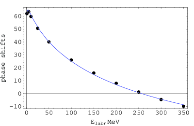
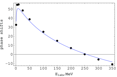
Here and are some constants. Being the generalization of the Yamaguchi model [10] to the case where the NN interaction is nonlocal in time, our model yields the nucleon-nucleon phase shifts in good agreement with experiment (see Figs.(1-3)). However, the main advantage of this model, is that it allows one to investigate the effects of the retardation in the NN interaction caused by the existence of the quark and gluon degrees of freedom on nucleon dynamics.
As we have seen, there is the one-to-one correspondence between the form of the generalized interaction operator and the UV behavior of the form factor In the case the operator would necessarily have the form (26). In this case the fundamental interaction is instantaneous. In the case (the restriction is necessary for the integral in (24) to be convergent), the only possible form of is (31), and, in the case , it must be of the form (35), and hence the interaction generating the dynamics of the system is nonlocal in time. Thus the interaction generating the dynamics can be nonlocal in time only if the form factors have the ”bad” large-momentum behavior that within Hamiltonian dynamics gives rise to the ultraviolet divergences:
From this it follows that the quark-gluon retardation effects must results in the ”bad” UV behavior of the matrix elements of the evolution operator as a function of momenta of hadrons. Note that EFT’s lead to the same conclusion:Within the EFT approach the quark and gluon degrees of freedom manifest themselves in the form of Lagrangians consistent with the symmetries of QCD which gives rise to the UV divergences. Note also that EFT’s are local theories, despite the existence of the external quark and gluon degrees of freedom. However, renormalization of EFT’s gives rise to the fact that these theories become nonlocal. Below this will be shown by using the example of our toy model.
As we have stated, the interaction operator (31) contains only one free parameter . However, if there is a bound state in the channel under study, then the parameter is completely determined by demanding that the T matrix has the pole at the bound-state energy. For example, in the channel the T matrix has a pole at energy MeV. This means that , and, by putting in Eq.(24), we get
| (36) |
In this case . Let us now show that renormalization of the LS equation with the separable potential leading to a logarithmic singularities produces the same T matrix. In [4] the problem of renormalization of the LS equation was considered by using the example of the separable potential
| (37) |
with . The corresponding T matrix is of the form (20) with
where the integral
has a logarithmic divergence. By using the dimensional regularization, one can get
where
The strength of the potential is adjusted to give the correct bound-state energy: In this way we get
| (38) |
The right-hand side of (38) is well-behaved in the limit . It is easy to see that, taking this limit, we get the expression (36) for . Thus renormalization of the LS equation with the above singular potential leads to the T matrix we have obtained by solving Eq.(13) with nonlocal-in-time interaction operator. This T matrix satisfies the generalized dynamical equation (13), but does not satisfy the LS equation. Correspondingly the Schrödinger equation is not valid in this case. The strength of the potential tends to zero as , and consequently the renormalized interaction Hamiltonian is also tend to zero. Thus despite the fact that the dynamics of each theory corresponding to the dimension is Hamiltonian dynamics for every , in the limiting case we go beyond Hamiltonian dynamics. The dynamics of the renormalized theory is governed by the generalized equation of motion (5) with nonlocal-in-time interaction operator which in the case of the model under study is given by (35).
IV Nonlocality in time of the NN interaction and an anomalous off-shell behavior of two-nucleon amplitudes.
As we have shown, renormalization in the model, in which the NN interaction is described by the singular potential, leads to the fact that the dynamics of the system is governed by the generalized dynamical equation with a nonlocal-in-time interaction operator, and in this way we get the same results we have obtained by using the model constructed within the GQD (in the case ). This is not surprising. In fact, Eq.(5) is a consequence of the most general physical principles, and must, for example, be satisfied in order that the evolution operator be unitary, and satisfy the composition law (2). Hence, the T matrix obtained by using a renormalization procedure must satisfy Eq.(13), provided this procedure leads to physically acceptable results, i.e. the theory is renormalizable. On the other hand the freedom in choosing the form of the interaction operator determining the boundary condition for Eq.(5) is limited by the condition (7),and, as we have seen, in the case of the form factors having the UV behavior (19) with , the interaction operator must be of the form (35) where only the parameter is free. However, in the case of the channel, this parameter is completely determined by demanding that the T matrix has a pole at energy . Thus we have a unique interaction operator satisfying the above requirements, the use of which in the boundary condition (14) for Eq.(13) leads to the same results as renormalization in the separable-potential model.
The main results of the above analyzes of the dynamical situation in the model under study is that renormalization gives rice to the fact that the dynamics of a quantum system is governed by the generalized dynamical equation (5) with nonlocal-in-time interaction operator. In Ref.[8] this fact has been shown, by using the example of the three-dimensional theory of a neutral scalar field interacting through a coupling. This gives reason to suppose that such a dynamical situation takes place in any renormalizable theory, for example, in an EFT. Below we will consider some general argument leading to this conclusion.
Let be the Green operator of a renormalizable theory corresponding to the momentum cutoff interaction Hamiltonian with renormalized constants. For every finite cutoff , the operator obviously satisfies the Hilbert identity (16)
| (39) |
At the same time, the renormalized Green operator is a limit of the consequence of the operators for . Since Eq.(39) is satisfied for every , and contains only the operator , the renormalized Green operator must also satisfy this equation
despite the fact that the renormalized Green operator cannot be represented in the form (17) (in the limit the operators do not converge to some operator acting on the Hilbert space). Correspondingly the renormalized T matrix satisfies Eqs.(13) and (15), despite the fact that in this case the LS and Schrödinger equations do not follow from these equations. Here the advantages of the GQD manifest themselves. Within the GQD the dynamical equation (5) are derived as consequences of the most general physical principles, and for Eq.(15) to be satisfied, the Green operator need not be represented in the form (17). In the GQD this operator is defined by (12), where the T matrix in turn is defined by (11), i.e. is expressed in terms of the amplitudes being the contributions to the evolution operator from the processes in which the interaction in a quantum system begins at time and ends at time . As we have shown, this allows one to use Eq.(5) and hence Eq.(13) as dynamical equations: Only in the case where the interaction operator is of the form (18), i.e. the dynamics of the system is Hamiltonian, the operator can be represented in the form (17). For every finite cutoff the dynamics of the system is Hamiltonian. At the same time, in the limiting case the dynamics is governed by the generalized dynamical equation with a nonlocal-in-time interaction operator, i.e. the dynamics is not Hamiltonian.
In order to clarify the characteristic features of the dynamics generated by the nonlocal-in-time interaction, let us come back to our toy model. In the Schrödinger picture, the evolution operator
of the model (33) can be rewritten in the form
| (40) |
where is given by (32). Since this T matrix satisfies Eqs.(13) and (15), the evolution operator (33) is unitary, and satisfies the composition law (2). Correspondingly, the operator constitute a one-parameter group of unitary operators, with the group property
| (41) |
Assume that this group has a self-adjoint infinitesimal generator which in the Hamiltonian formalism is identified with the total Hamiltonian. Then for we have
| (42) |
From this and (41) it follows that
where
| (43) |
Since is an analytic function of , and, in the case , tends to zero as , from (44) we get for any and , and hence . This means that, if the infinitesimal generator of the group of the operators exists, then it coincides with the free Hamiltonian, and the evolution operator is of the form . Thus, since this, obviously, is not true, the group of the operators has no infinitesimal generator, and hence the dynamics is not governed by the Schrödinger equation.
It should be also noted that in the case , is not an operator on the Hilbert space. In fact, the function
| (44) |
is not square integrable for any nonzero , because of the slow rate of decay of the form factor as . Correspondingly, the T matrix given by (32) does not represent an operator on the Hilbert space. However, as we have stated, in general may be only an operator-valued generalized function such that the evolution operator is an operator on the Hilbert space. Correspondingly, the T matrix must be such that given by (12) is an operator on the Hilbert space. In our model, and the T matrix satisfy these requirements, since the evolution operator given by (33) and the corresponding are operators on the Hilbert space. At the same time, in this case we go beyond Hamiltonian dynamics.
We have shown that after renormalization nucleon dynamics is governed by the generalized dynamical equation (5) with a nonlocal-in-time interaction operator. The analyzes of the dynamical situation arising due to the existence of the external quark and gluon degrees of freedom leads to the same conclusion. As we have shown by using our toy model, such a nonlocality of the NN interaction can have significant effects on the character of nucleon dynamics. As is well known, the dynamics of many nucleon systems depends on the off-shell properties of the two-nucleon amplitudes. For this reason, let us consider the effects of the nonlocality of the NN interaction on these properties.
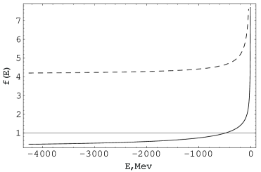
In the nonlocal case, the matrix elements of the evolution operator as functions of momenta do not go to zero at infinity so fast as it is required by ordinary quantum mechanics, and within the Hamiltonian formalism this leads to the ultraviolet divergences. For example, in this case the two-nucleon amplitudes do not go to zero fast enough to make the Faddeev equation well-behaved. Note that the same problem arises in the EFT approach. Another consequence of nonlocality in time of the interaction is that for fixed momenta and the matrix elements tend to zero as , while, in the local case, they tend to in this limit. To illustrate this, we present in Fig.4 the off-shell behavior of in the limit . Thus, nonlocality in time of the interaction caused by the existence of the quark and gluon degrees of freedom gives rise to an anomalous off-shell behavior of the two-nucleon amplitudes. The off-shell properties of the amplitudes for the ordinary interaction operator and the operator containing the nonlocal term are qualitatively different. This is true even when the two interaction operators have approximately the same phase shifts. Such a large variation in the off-shell behavior of the amplitudes, even when the interaction operators are identical on-shell, can have significant effects on three- and many-body results [10]. This gives reason to expect that the anomalous off-shell behavior of the two-nucleon amplitudes can also have significant effects on nucleon matter properties.
V Conclusion.
By using the model of the separable NN potential which gives rise to logarithmic singularities in the Born series, we have demonstrated that after renormalization the dynamics of a nucleon system is governed by the generalized dynamical equation (5) with a nonlocal in time interaction operator. By using Eq.(16) we have shown that this should be true in the general case. At the same time, being very simple and exactly solvable, the toy model allows one to investigate some characteristic features of the dynamics of a theory after renormalization. We have shown that the dynamical situation in the toy model which arises after renormalization is completely unsatisfactory from the point of view of the Hamiltonian formalism: The group of the evolution operators has no infinitesimal generator, and hence the Hamiltonian of the renormalized theory cannot be defined. On the other hand, as has been shown in Ref.[3] , the current concepts of quantum theory allow the extension of quantum dynamics to the case where the group of the evolution operator has no infinitesimal generator (in this case the interaction generating the dynamics of a system is nonlocal in time). The Schrödinger equation is only a particular case of the generalized dynamical equation (5) derived as a consequence of the most general principles of quantum theory, and there are no reasons to restrict ourselves to the local case where the interaction is instantaneous and the evolution operator has an infinitesimal generator. Moreover, in quantum field theory such a restriction gives rise to the UV divergences, and, as has been shown, after renormalization the dynamics of a theory is not Hamiltonian. At the same time, we have shown that such a dynamics is governed by the generalized dynamical equation (5) with a nonlocal-in-time interaction operator. This means that the GQD provides the extension of quantum dynamics which is needed for describing the evolution of quantum systems within a renormalized theory. This gives reason to hope that the use of the GQD and parameterization of the NN forces like (35) can open new possibilities for applying the EFT approach to the description of low-energy nucleon dynamics. By using an EFT, one can construct the generalized interaction operator consistent with the symmetries of QCD. This operator can then be used in Eq.(5) for describing nucleon dynamics. Note that in this case regularization and renormalization are needed only on the stage of determining the generalized interaction operator. After this one does not face the problem of UV divergences.
References
- (1) S. Weinberg, Physica A 96 327 (1979); E. Witten, Nucl. Phys. B 122 109 (1977); H. Georgi, Annu. Rev. Nucl. Part. Sci. 43 209 (1993); J. Polchinski, Proceedings of Recent Directions in Particle Theory TASI-92 235 (1992); A.V. Manohar, hep-ph/9508245; D.B. Kaplan, nucl-th/9506035.
- (2) T. Mehen and I.W. Stewart, Phys. Rev. C 59 2365 (1998); C. Ordonez, and U. van Kolck, Phys. Lett. B 291 459 (1992); U. van Kolck, Phys. Rev. C 49 2932 (1994); D.B. Kaplan, M.J. Savage, and M.B. Wise, Phys. Lett. B 424 390 (1998); Nucl. Phys. B 534 329 (1998).
- (3) R.Kh. Gainutdinov, J. Phys. A 32, 5657 (1999).
- (4) R.P. Feynman, Rev. Mod. Phys. 20, 367 (1948).
- (5) D.R. Phillips, I.R. Afnan, and A.G. Henry-Edwards, Phys. Rev. C. 61, 044002-1 (2000).
- (6) R.Kh. Gainutdinov and A.A. Mutygullina, Yad. Fiz. 60, 938 (1997).
- (7) R.Kh. Gainutdinov and A.A. Mutygullina, Yad. Fiz. 62, 2061 (1999).
- (8) V.G.J. Stoks, R.A.M. Klomp, M.C.M. Rentmeester, and J.J. de Swart, Phys. Rev. C 48, 792 (1993).
- (9) R. Kh. Gainutdinov, hep-th/0107139.
- (10) Y.Yamaguchi, Phys. Rev. 95, 1635 (1954).
- (11) R. Machleidt, F. Sammarruca, and Y. Song, Phys. Rev. C 53, 1483 (1996); A. D. Lahiff and I. R. Afnan, Phys. Rev. C 56, 2387 (1997).